Increasing Scalability of Process Mining using Event Dataframes: How Data Structure Matters

In this section, the notion of event log, i.e., a collection of events recorded in the execution of a business process that is the starting point of many process mining analysis, is formally introduced. For the following definition, let $\mathcal{U}_{E}$ be the universe of events, $\mathcal{U}_{C}$ be the universe of case identifiers, $\mathcal{U}_{A}$ be the universe of activities (names referring to a particular step of a process), $\mathcal{U}_{\textrm{attr}}$ be the universe of attribute names (all the names of the attributes that can be related to an event), $\mathcal{U}_{\textrm{val}}$ be the universe of attribute values (all the possible values for attributes).

This classical event log notion matches the XES storage format [19], that is the common source of information for process mining tools like Disco, ProcessGold, Celonis, QPR, Minit, …An example attribute of an event $e$ is the timestamp $\textrm{attr}(e)(time)$ which refer to the time the event happened. While, in general, an event belongs to a single case, in Def. 1 the function case_ev might be such that cases share events.

An important consideration is that for an event $e\in E$, applying attr, the resulting mapping $\mathcal{U}_{attr}\not\rightarrow\mathcal{U}_{val}$ is a partial function. This means that not all the attributes are valued for all the events, e.g., there might be some attributes that are specific for a single event.

The Directly-Follows Graph (DFG) is a basic representation of the activities of the process, that are connected with a directed if they follow each other in at least an instance of the event log. The DFG is usually annotated by the number of occurrences for each edge (corresponding to the number of occurrences of the log where an activity has been followed by another activity in the log).

The concept of a Directly-Follows Graph is formally introduced in the following definition:

Let $\textrm{start}_{\textrm{DFG}}\subseteq N_{\textrm{DFG}}$ be the subset of start activities in the log, and $\textrm{end}_{\textrm{DFG}}\subseteq N_{\textrm{DFG}}$ be the subset of end activities in the log. Then, the DFG structure can be converted into a Petri net useful for conformance checking purposes using the method described in [14]. Moreover, a variant of the Inductive Miner (IMDF) is described in [13].

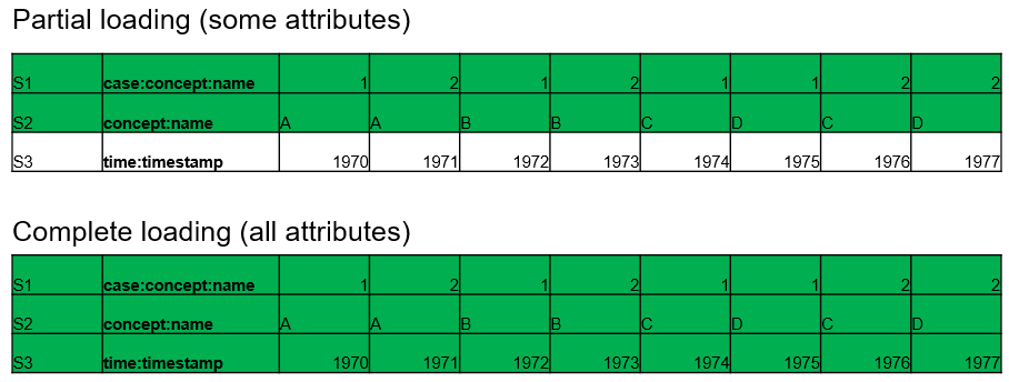
This section will introduce row- and columnar-based storages. While the remainder of the paper will be mainly focused on columnar storages and data structures, it is interesting to see how modern row-based storages cope against the columnar storages when saving process mining event logs.

Row-based storage systems are optimized to read logs ‘‘by rows’’, ‘‘by events’’: while parsing, the row is considered in its entirety, and all the values for all the attributes of the parsed event are read at first glance. A well-known row-based storage format is the Avro format¹¹ 1 https://avro.apache.org/. Each Avro file contains an header, where the parsing schema is defined, and one or more data blocks (containing one or more rows). For process mining purposes, the event log can be transformed into a list of events, and then each event serialized into a row.

Column-based storage systems are optimized to read logs by “by columns”, making possible to choose which attributes are needed before starting to load the file (see Figure 1). In this way, only the values of some attributes are parsed, making the load operation faster. Since each column of the file contains data of the same format (integer, string, …), more effective compression techniques can be deployed. Among the compression algorithms supported by Parquet, there is the Snappy compression²² 2 https://en.wikipedia.org/wiki/Snappy_(compression) and the Gzip compression³³ 3 https://en.wikipedia.org/wiki/Gzip. Snappy is more fast in compressing/decompressing, while Gzip obtains better compression ratios at the expense of performance. Apache Parquet⁴⁴ 4 https://parquet.apache.org/ is supported by a large number of big data frameworks (Apache Hive, Apache Drill, Apache Impala, Apache Pig, Apache Spark, Cascading, …). Apache ORC⁵⁵ 5 https://orc.apache.org/ is an alternative in the columnars. In Table 2, the size on disk of the logs stored in the different formats is reported. The Apache Parquet format with the Gzip compression achieves the best results in terms of log size on disk, while Parquet with the Snappy compression remains very efficient while avoiding the compression/decompression performance deficit of Gzip.

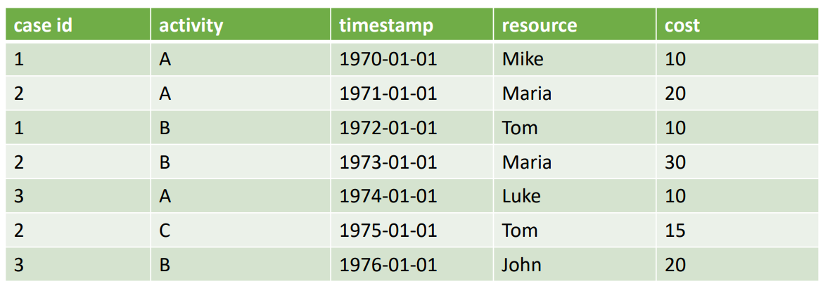
To introduce the concept of dataframe, one could think to a set of attribute names (columns) associated to the values (of the attribute) for each row (that is an event). An example representation is contained in Fig. 2.

In the following, we consider $\mathcal{U}_{D}$ to be the universe of dataframes, and $\chi^{\textrm{val}}:N\rightarrow I\times(P\cup\{\epsilon\})$ is a function that associates to an attribute name the set of all indexed values, i.e., for $n\in N$: $\chi^{\textrm{val}}(n)=\cup_{i\in I}\{(i,\chi^{\textrm{val}}_{i}(n))\}$. Hence, if we take the second element of the couples, we get the set of all attribute values for $n$, that we indicate with $\pi_{2}(\chi^{\textrm{val}}(n))$. Moreover, given a dataframe $D\in\mathcal{U}_{D}$, the function $\pi_{I}:\mathcal{U}_{D}\rightarrow\mathcal{P}(\mathbb{N})$, $\pi_{I}((I,N,T,V,\chi^{\textrm{val}}_{i},\chi^{\textrm{type}}))=I$ is defined.

The data structure defined in subsection 5.1 is actually an abstraction of the one that is implemented in Pandas (Python) and Apache Spark. In this section, we want to describe a simple implementation of the dataframe concept, assuming that the name of the attributes is represented as a string. The proposed implementation is the following: Map$<$String, ArrayList$<$Object$>>$ where: Map is any associative array implementation⁶⁶ 6 https://en.wikipedia.org/wiki/Associative_array and ArrayList is any dynamic array implemented⁷⁷ 7 https://en.wikipedia.org/wiki/Dynamic_array. In the previous data structure, all the values for a particular attribute can be retrieved from the map as an array list of objects. In this data structure, the value in position $i$ is the value of the attribute for the event at position $i$ in the dataframe.

Converting from an event log $L=(C_{I},E,A,\textrm{case\_ev},\allowbreak\textrm{act},\allowbreak\textrm{attr},\leq)$ to a dataframe $D=(I,N,T,V,\chi^{\textrm{val}}_{i},\chi^{\textrm{type}})$ requires the assumption that an attribute $n_{\textrm{case}}\in\mathcal{U}_{\textrm{attr}}$ exists in the domain of $\textrm{attr}(e)$ for each event $e\in E$. Since $\leq$ (see 1) is a total order on $E$, $E$ can be viewed as a sequence of events, $E=\{e_{1},e_{2},\ldots,e_{n}\}$, such that $e_{i}\leq e_{j}$ if and only if $i\leq j$. The conversion is such that $N=\mathcal{U}_{attr}$ is the set of attributes of the dataframe, and $T=\{o\}$ can be defined to contain a single (object) type. Then, $V=\cup_{e\in E}\textrm{Im}~\textrm{attr}(e)$, $\chi^{\textrm{type}}(n)=t~\forall n\in N$, and

We introduce the following functions in order to be able to perform process mining operations on top of a dataframe (as the calculation of Directly-Follows Graphs). These functions transform a/some dataframe(s) into another dataframe.

• •

  Projection on a given expression: given a dataframe $D=(I,N,T,V,\chi^{\textrm{val}}_{i},\chi^{\textrm{type}})$, a set of attribute names $S\subseteq N$ and a function $f:I\times\mathcal{P}(N)\rightarrow\{0,1\}$ (selective function based on the attribute values), a projection function is defined as $\textrm{proj}((I,N,T,V,\chi^{\textrm{val}}_{i},\chi^{\textrm{type}}),S,f)=(I^{\prime},N,T,V,\chi^{\prime\textrm{val}}_{i},\chi^{\textrm{type}})$ where $I^{\prime}=\{i\in I,f(i,S)=1\}$ and $\chi^{\prime\textrm{val}}_{i}(n)=\chi^{\textrm{val}}_{i}(n)$   for all $i\in I^{\prime}$ and $n\in N$.

• •

  Grouping function: the grouping function is defined given a dataframe $D=(I,N,T,V,\chi^{\textrm{val}}_{i},\chi^{\textrm{type}})\in\mathcal{U}_{D}$ and an attribute $n_{0}\in N$ as

  $$\textrm{group}(D,n_{0})=\bigcup_{v\in\pi_{2}(\chi^{\textrm{val}}(n_{0}))}\textrm{proj}(D,n_{0},\{v\})$$

  by construction, $\textrm{proj}(D,n_{0},\{v\})\cap\textrm{proj}(D,n_{0},\{v^{\prime}\})=\emptyset$ if $v\neq v^{\prime}$, so the sets are pairwise disjoint.

• •

  Shift function: $\textrm{shift}((I,N,T,V,\chi^{\textrm{val}}_{i},\chi^{\textrm{type}}))=(I^{\prime},N,T,V,\chi^{\prime\textrm{val}}_{i},\chi^{\textrm{type}})$ where $I^{\prime}=\{i-1\arrowvert i\in I\}$, $\chi^{\prime\textrm{val}}_{i-1}(n)=\chi^{\textrm{val}}_{i}(n)$   $\forall i\in I,n\in\mathbb{N}$.

• •

  Concatenation function: for $D_{1}=(I_{1},N_{1},T_{1},V_{1},\chi^{\prime\textrm{val}}_{i},\chi^{\prime\textrm{type}})\in\mathcal{U}_{D}$, $D_{2}=(I_{2},N_{2},T_{2},V_{2},\chi^{\prime\prime\textrm{val}}_{i},\chi^{\prime\prime\textrm{type}})\in\mathcal{U}_{D}$, and $s\in\Sigma$ such that $\{n_{2}\oplus s\arrowvert n_{2}\in N_{2}\}\cap N_{1}=\emptyset$, the concatenation is defined as $\textrm{concat}(D_{1},D_{2},s)=(I,N,T,V,\chi^{\textrm{val}}_{i},\chi^{\textrm{type}})$ where $I=I_{1}\cup I_{2}$, $N=N_{1}\cup\{n_{2}\oplus s\arrowvert n_{2}\in N_{2}\}$, $T=T_{1}\cup T_{2}$, $V=V_{1}\cup V_{2}$,

  $${\scriptscriptstyle\chi^{\textrm{val}}_{i}(n)=\begin{cases}\chi^{\prime\textrm{val}}_{i}(n)&n\in N_{1}\\ \chi^{\prime\prime\textrm{val}}_{i}(n^{\prime})&n=n^{\prime}\oplus s,n^{\prime}\in N_{2}\\ \end{cases}\hskip 7.3612pt\chi^{\textrm{type}}(n)=\begin{cases}\chi^{\prime\textrm{type}}(n)&n\in N_{1}\\ \chi^{\prime\prime\textrm{type}}(n^{\prime})&n=n^{\prime}\oplus s,n^{\prime}\in N_{2}\\ \end{cases}}$$

• •

  Sorting function: let $D=(I,N,T,V,\chi^{\textrm{val}}_{i},\chi^{\textrm{type}})$ be a dataframe and $n\in N$ an attribute name. Let $b_{n}:I\rightarrow\{1,\ldots,\arrowvert I\arrowvert\}$ a bijection such that:

  • –

    If $\chi^{\textrm{val}}_{i}(n)\leq_{V}\chi^{\textrm{val}}_{j}(n)$ according to the partial order defined on $V$, then $b_{n}(i)\leq_{\mathbb{N}}b(j)$.

  • –

    If $\chi^{\textrm{val}}_{i}(n)\leq_{V}\chi^{\textrm{val}}_{j}(n)\wedge\chi^{\textrm{val}}_{j}(n)\leq_{V}\chi^{\textrm{val}}_{i}(n)$, then $b_{n}(i)\leq_{\mathbb{N}}b(j)\iff i\leq_{\mathbb{N}}j$.

  With this definition, $\textrm{sort}(D,n,b)=(\{1,\ldots,\arrowvert I\arrowvert\},N,T,V,\chi^{\prime\textrm{val}}_{i},\chi^{\textrm{type}})$ could be introduced as $\chi^{\prime\textrm{val}}_{b_{n}(i)}(n)=\chi^{\textrm{val}}_{i}(n)$.

• •

  String attribute merging: let $D=(I,N,T,V,\chi^{\textrm{val}}_{i},\chi^{\textrm{type}})$ be a dataframe, then a new attribute $n\in\mathcal{U}_{\textrm{attr}}$ of type $\textrm{str}\in\mathcal{U}_{T}$ could be inserted into the dataframe as merge of the values of two (existing) attributes $n_{1},n_{2}\in N$ (separated by a string delimiter $s$) to obtain a new dataframe

  $$\textrm{mergstrv}(D,n,n_{1},n_{2},s)=(I,N^{\prime},T,V^{\prime},\chi^{\prime\textrm{val}}_{i},\chi^{\prime\textrm{type}})$$

  where: $N^{\prime}=N\cup\{n\}$ and $V^{\prime}=V\bigcup\cup_{i\in I}\{\chi^{\textrm{val}}_{i}(n_{1})\oplus s\oplus\chi^{\textrm{val}}_{i}(n_{2})\}$

In this section, we want to show that it’s actually possible to calculate the Directly-Follows Graph (DFG; see subsection 3.2) on top of the dataframe structures. Let $D=(I,N,T,V,\chi^{\textrm{val}}_{i},\chi^{\textrm{type}})$ be a dataframe. Let $n_{\textrm{case}}\in N$ be the case identifier attribute, and $n_{\textrm{act}}\in N$ be the attribute that identifies the activity. The nodes of the DFG are simply the different values for the activities: $\pi_{2}(\chi^{\textrm{val}}(n_{\textrm{act}}))$. For the retrieval of the edges and the count, two different strategies are actually possible:

• •

  Map-reduce: the dataframe is grouped using the $n_{\textrm{case}}$ attribute, and then the edges and the counts are retrieved as:

  $${\scriptstyle E=\bigcup_{G\in\textrm{group}(D,n_{\textrm{case}})}\bigcup_{(i,j)\in\pi_{I}(G)^{2},i<j\wedge\not\exists k\in\pi_{I}(G),i<k<j}\left\{\left(\chi^{\textrm{val}}_{i}(n_{\textrm{act}}),\chi^{\textrm{val}}_{j}(n_{\textrm{act}})\right)\right\}}$$

  For $e\in E$,

  $${\scriptstyle c(e)=\sum_{G\in\textrm{group}(D,n_{\textrm{case}})}\sum_{(i,j)\in\pi_{I}(G)^{2},i<j\wedge\not\exists k\in\pi_{I}(G),i<k<j}\mathbbm{1}_{(\chi^{\textrm{val}}_{i}(n_{\textrm{act}}),\chi^{\textrm{val}}_{j}(n_{\textrm{act}}))=e}}$$

  In a map-reduce implementation, the grouping is performed and then different groups can be assigned to different workers (map phase). The single results are then merged in the reduce phase to obtain the final result.

• •

  Shifting and counting: the strategy assumes that the dataframe is sorted the strategy could be explained as follows:

  1. 1.

     A shifted version of the dataframe is obtained using the shift function.

  2. 2.

     Then, a concatenated dataframe is obtained as: $D^{\prime}=(I^{\prime},N^{\prime},T^{\prime},V^{\prime},\chi^{\prime\textrm{val}}_{i},\chi^{\prime\textrm{type}})=\textrm{concat}(D,\textrm{shift}(D),\textrm{"\_2"})$.

  3. 3.

     Then, if $n_{\textrm{case}}$, $n^{\prime}_{\textrm{case}}$ are the attributes identifying the case respectively in $D$ and $D^{\prime}$, a dataframe $D^{\prime\prime}$ could be obtained taking $S=\{n_{\textrm{case}},n^{\prime}_{\textrm{case}}\}$, and $f:I\times\mathcal{P}(N)\rightarrow\{0,1\}$ such that $f(i,S)=\mathbbm{1}_{\chi^{\prime\textrm{val}}_{i}(n_{\textrm{case}})=\chi^{\prime\textrm{val}}_{i}(n^{\prime}_{\textrm{case}})}$, as $D^{\prime\prime}=(I^{\prime\prime},N^{\prime},T^{\prime},V^{\prime},\chi^{\prime\prime\textrm{val}}_{i},\chi^{\prime\textrm{type}})=\textrm{proj}(D^{\prime},S,f)$. In such way, only rows in the concatenated dataframe that have the same case ID are kept.

  4. 4.

     Eventually, a new dataframe with an additional column $n^{\prime\prime}_{\textrm{act}}$ can be defined starting from $D^{\prime\prime}$, if $n_{\textrm{act}}$, $n^{\prime}_{\textrm{act}}$ are the attributes identifying the activity respectively in $D$ and $D^{\prime}$, as:

     $$D^{\prime\prime\prime}=(I^{\prime\prime\prime},N^{\prime\prime},T^{\prime\prime},V^{\prime\prime},\chi^{\prime\prime\prime\textrm{val}}_{i},\chi^{\prime\prime\textrm{type}})=\textrm{mergstrv}(D^{\prime\prime},n^{\prime\prime}_{\textrm{act}},n_{\textrm{act}},n^{\prime}_{\textrm{act}},\textrm{","})$$

  5. 5.

     The edges and the count of the DFG are: $E=\pi_{2}(\chi^{\prime\prime\prime\textrm{val}}(n^{\prime\prime}_{\textrm{act}}))$ and $c:E\rightarrow\mathbb{N},c(e)=\arrowvert\{i\in I\arrowvert\chi^{\prime\prime\prime\textrm{val}}_{i}(n^{\prime\prime}_{\textrm{act}})=e\}\arrowvert$

A representation of the ideas underlying the algorithm is contained in Figure 3.

Filtering: Filtering on the attribute values of events is an ubiquitous operation in process mining, since only a part of the events of the log may be of interest for an analysis. Even in the worst case, accessing the value of an attribute for an event has $O(1)$ complexity, hence filtering a dataframe with $N$ events has a complexity that is in the worst case equal to $O(N)$. A comparison between the complexity of filtering on event logs and dataframe implementations is contained in Table 3.

Directly-Follows Graph computation: the computation of the DFG on top of classical event logs requires a single iteration on the log and the storage of the DFG edges in a map. Hence, the complexity is $O(N)$ in the average case and $O(N^{2})$ in the worst case where all the events belong to the same case and a lot of collisions happen in the map. As seen in subsection 5.4, there are two ways to calculate the DFG on top of dataframes: map-reduce, and “shifting and counting”.

For the map-reduce approach, the complexity is still $O(N)$ in the average case because all the operations involved (grouping, mapping and reducing to the map of edges and counts) have a linear average complexity. The reduce approach, in the worst case, can have $O(N^{2})$ complexity when a lot of collisions inside the map happen. However, the real-life map-reduce implementations on dataframes (Pandas, Spark) are disappointing, being slow in the map operation and/or hampered by network traffic issues (when the computations are split between different nodes)

For the “shifting and counting” approach, the initial sort on the dataframe has a complexity (if algorithms like mergesort and heapsort are used) equal to $O(N*log(N))$ in the average and worst case. Then, every remaining operation has linear complexity, hence excluding the sorting operation, the complexity of the remaining operations is still $O(N)$ in the average case, and $O(N^{2})$ in the worst (that happens when a lot of collisions happen in writing the edges and their count in the map).

To recap, the main difference between classical event logs and dataframes is the way attributes at event level are accessed:

• •

  On classical event logs, the attribute map of the event is retrieved, and a specific key of the map is accessed to retrieve the value of the attribute.

• •

  On dataframes, the list of values for the specific attribute is retrieved, and then a specific index (corresponding to the index of the row/event) is retrieved.

A comparison between the filtering complexity on classical event logs and dataframe implementations is contained in Table 4.

References

- [1] van der Aalst, W., Damiani, E.: Processes meet big data: Connecting data science with process science. IEEE Transactions on Services Computing 8(6) (2015)
- [2] Abadi, D., Boncz, P., Harizopoulos, S., Idreos, S., Madden, S., et al.: The design and implementation of modern column-oriented database systems. Foundations and Trends® in Databases 5(3), 197–280 (2013)
- [3] Abadi, D.J., Madden, S.R., Hachem, N.: Column-stores vs. row-stores: how different are they really? In: Proceedings of the 2008 ACM SIGMOD international conference on Management of data. pp. 967–980. ACM (2008)
- [4] Adriansyah, A., van Dongen, B., van der Aalst, W.: Conformance checking using cost-based fitness analysis. In: 2011 IEEE 15th International Enterprise Distributed Object Computing Conference. pp. 55–64. IEEE (2011)
- [5] Augusto, A., Conforti, R., Dumas, M., La Rosa, M., Maggi, F.M., Marrella, A., Mecella, M., Soo, A.: Automated discovery of process models from event logs: Review and benchmark. IEEE Transactions on Knowledge and Data Engineering 31(4), 686–705 (2018)
- [6] Azzini, A., Ceravolo, P.: Consistent process mining over big data triple stores. In: 2013 IEEE International Congress on Big Data. pp. 54–61. IEEE (2013)
- [7] Berti, A., van Zelst, S.J., van der Aalst, W.: PM4Py Web Services: Easy Development, Integration and Deployment of Process Mining Features in any Application Stack. In: BPM Demo Track (2019)
- [8] Berti, A., van Zelst, S.J., van der Aalst, W.: Process Mining for Python (PM4Py): Bridging the Gap Between Process-and Data Science. In: ICPM Demo Track (CEUR 2374). pp. 13–16 (2019)
- [9] Cheng, L., Van Dongen, B., Van Der Aalst, W.: Scalable Discovery of Hybrid Process Models in a Cloud Computing Environment. IEEE Transactions on Services Computing (2019)
- [10] van Dongen, B.F., Shabani, S.: Relational XES: Data Management for Process Mining. In: CAiSE Forum. pp. 169–176 (2015)
- [11] Hernández, S., van Zelst, S.J., Ezpeleta, J., van der Aalst, W.: Handling Big (ger) Logs: Connecting ProM 6 to Apache Hadoop. In: BPM (Demos). pp. 80–84 (2015)
- [12] Leemans, S.J., Fahland, D., van der Aalst, W.: Discovering block-structured process models from event logs-a constructive approach. In: International conference on applications and theory of Petri nets and concurrency. Springer (2013)
- [13] Leemans, S.J., Fahland, D., van der Aalst, W.: Scalable process discovery and conformance checking. Software & Systems Modeling 17(2), 599–631 (2018)
- [14] Leemans, S.J., Poppe, E., Wynn, M.T.: Directly follows-based process mining: Exploration & a case study. In: Proceedings of the ICPM International Conference on Process Mining, Aachen, Germany. p. 46 (2019)
- [15] Loreti, D., Chesani, F., Ciampolini, A., Mello, P.: Distributed compliance monitoring of business processes over mapreduce architectures. In: Proceedings of the 8th ACM/SPEC on International Conference on Performance Engineering Companion. pp. 79–84. ACM (2017)
- [16] Mannhardt, F.: XESLite-managing large XES event logs in ProM. BPM Center Report BPM-16-04 pp. 224–236 (2016)
- [17] Syamsiyah, A., van Dongen, B., van der Aalst, W.M.: Db-xes: enabling process discovery in the large. In: International Symposium on Data-Driven Process Discovery and Analysis. pp. 53–77. Springer (2016)
- [18] Valdivieso, H., Lee, W.L.J., Munoz-Gama, J., Sepúlveda, M.: OpyenXES: A Complete Python Library for the eXtensible Event Stream Standard pp. 71–75 (2018)
- [19] Verbeek, H., Buijs, J.C., Van Dongen, B., van der Aalst, W.: Xes, xesame, and prom 6. In: International Conference on Advanced Information Systems Engineering. pp. 60–75. Springer (2010)