Optimal Dynamic Multi-Resource Management in Earth Observation Oriented Space Information Networks

Yu Wang, Min Sheng, , Qiang Ye, ,
Shan Zhang, Weihua Zhuang, , Jiandong Li,

Abstract

Space information network (SIN) is an innovative networking architecture to achieve near-real-time mass data observation, processing and transmission over the globe. In the SIN environment, it is essential to coordinate multi-dimensional heterogeneous resources (i.e., observation resource, computation resource and transmission resource) to improve network performance. However, the time varying property of both the observation resource and transmission resource is not fully exploited in existing studies. Dynamic resource management according to instantaneous channel conditions has a potential to enhance network performance. To this end, in this paper, we study the multi-resource dynamic management problem, considering stochastic observation and transmission channel conditions in SINs. Specifically, we develop an aggregate optimization framework for observation scheduling, compression ratio selection and transmission scheduling, and formulate a flow optimization problem based on extended time expanded graph (ETEG) to maximize the sum network utility. Then, we equivalently transform the flow optimization problem on ETEG as a queue stability-related stochastic optimization problem. An online algorithm is proposed to solve the problem in a slot-by-slot manner by exploiting the Lyapunov optimization technique. Performance analysis shows that the proposed algorithm achieves close-to-optimal network utility while guaranteeing bounded queue occupancy. Extensive simulation results further validate the efficiency of the proposed algorithm and evaluate the impacts of various network parameters on the algorithm performance.

Index Terms:

Space information network, time-varying channel, scheduling, time expanded graph, stochastic optimization, multi-dimensional resource, Earth observation.

I Introduction

It is well recognized that Earth observation plays an indispensable role in realizing a plethora of applications, e.g., environment monitoring, weather forecast, target surveillance, and disaster relief [1, 2]. Everyday, huge volumes of data (e.g., some 700 Gbytes of data daily for ALOS [3]) are generated by versatile applications, which leads us to the era of big Earth observation data [4]. To accommodate the ever-increasing Earth observation demands, the space information network (SIN) [5, 6, 7, 8, 9] stands out as a promising solution by integrating multi-layered heterogeneous space platforms such as geostationary Earth orbit (GEO) satellites, low Earth orbit (LEO) satellites, high-altitude platforms, and so on. Through SIN, it is feasible to achieve near-real-time mass data acquisition, processing and transmission [10].

In the dynamic and complex SIN environment, multi-resource needs to be well coordinated for cooperative Earth observation [11]. Specifically, to fulfill an Earth observation task, observation, computation and transmission resources are required. However, the multi-dimensional heterogeneous resources are normally unbalanced and constrained in SINs. This constraint can lead to a dilemma that the captured large-volume observation data cannot be transmitted to specified destinations in due time. To address the issue, several offline multi-resource coordinate scheduling algorithms have been proposed in the literature [12, 13, 14, 15, 11]. Particularly, the joint observation and transmission scheduling problem for the COSMO-SkyMed constellation is first introduced in [12]. In [13], a constraint satisfaction optimization model is used to describe Earth observation satellite (EOS) observation tasks and data transmission jobs in an integrated way, and a genetic algorithm based meta-heuristic is proposed. In our earlier studies, we exploit an extended time expanded graph (ETEG) method and propose an analytical framework to characterize multi-resource evolution in the complex and dynamic SIN environment [14, 15]. As an extension, multi-resource coordinate scheduling problem is studied and an iterative optimization technique with low complexity is applied to efficiently solve the problem in [11].

The multi-dimensional resources normally exhibit time varying characteristics in the SIN context. To be specific, on one hand, for the observation resource, the resultant image quality depends heavily on the weather condition of the target area at the time of taking images. An imaging request for a certain observation area may fail due to bad weather conditions (raining or with cloud coverage) over that area [16]. On the other hand, for the transmission resource, the satellite downlink contact capacity changes with time due to physical phenomena related to the propagation of radiowaves through the atmosphere, especially for satellite communication systems operating at Ku, Ka and V frequency bands. Further, the capacity of intersatellite contacts also changes due to varying distance, noise and interference [17, 18, 19]. The above observations have given rise to the need for efficient multi-resource management while considering the time varying property of different resources.

It is technically challenging to develop dynamic multi-resource coordination strategies for SINs, due to several reasons: 1) Highly dynamic network topology [20, 21]. The continuously changing network topology brings a resource availability issue. A certain type of resource (e.g., observation resource) is usable only when two related nodes are within the line-of-sight range. Besides, the resource combinations to accomplish a task are highly complex. As a consequence, it is difficult to model the multi-resource correlation relationship in the presence of topology dynamics; 2) Multi-resource conflicts [22, 23, 24]. Both the observation and transmission resources are limited in SINs. These multi-resource limitations can lead to infeasibility of all potential observation and transmission opportunities, and thus induce observation and transmission conflicts. To make matter worse, the above conflicts can change in a small time period due to the dynamic network topology evolution; and 3) Balancing the stochastic observation and transmission processes. Since both the observation process and transmission process exhibit time varying characteristics, it is difficult to match the two stochastic processes without prior knowledge of channel state distribution.

In this paper, to address the technical challenges, we study the multi-dimensional resource dynamic management problem for SINs, while taking into account both the observation and transmission channel variations. Specifically, we first employ an ETEG to characterize multi-resource correlation relationships in the dynamic SIN context. On the basis of ETEG, an aggregate optimization framework is developed for observation scheduling, compression ratio selection and transmission scheduling, and a constrained flow optimization problem is formulated to maximize the sum network utility. We then transform the optimization problem on ETEG as a queue stability-related stochastic optimization problem on a multi-queue multi-server queueing model. By exploiting the Lyapunov optimization technique, an online algorithm, i.e., Dynamic Multi-Resource Cooperation (DMRC) algorithm, is proposed to decompose the optimization problem into separate joint observation scheduling and adaptive processing subproblem and transmission scheduling sub-problem. For the first sub-problem, we utilize the Lagrangian dual theory to optimally solve the transformed convex optimization problem. For the second sub-problem, we transform it into the maximum weighted matching problem in a constructed bipartite graph. The computational complexity and theoretical performance bound of the proposed DMRC algorithm are analyzed in detail. We show that the DMRC algorithm can achieve network utility arbitrarily close to the optimal value without requiring the prior knowledge of channel conditions. Extensive simulation results are provided to demonstrate the efficiency of the proposed algorithm and evaluate the impacts of various network parameters on the algorithm performance.

In a nutshell, the main contributions of this paper are summarized as follows:

1.

An optimization framework of observation scheduling, adaptive compression and transmission scheduling based on ETEG is formulated to maximize the sum network utility;
2.

We equivalently transform the constrained flow optimization problem on ETEG as a queue stability-related stochastic optimization problem by exploiting a multi-queue multi-server queueing model;
3.

We use the Lyapunov optimization method to solve the optimization problem. The performance bound of the proposed DMRC algorithm is theoretically analyzed and proved to be arbitrarily close to the optimality.

The remainder of this paper is organized as follows. Section II introduces the SIN system model under consideration and Section III elaborates on the detailed problem formulation and transformation. We propose an approximate online multi-resource dynamic scheduling algorithm and analyze its complexity as well as performance bound in Section IV. The performance evaluation by simulations is presented in Section V, followed by concluding remarks and future research in Section VI.

II System Model

In this section, we first introduce the SIN network model under consideration. Then, an ETEG model is employed to describe the multi-resource correlation relationship over the network.

II-A Network Model

Consider a satellite-based SIN system operating in slotted time $t\in\mathcal{T}=\{1,2,...\}$ [25]. The length of a time slot is denoted as $\tau$ . There are three different types of components in the SIN: 1) a set, $\mathcal{I}=\{1,2,\ldots,I\}$ , of $I$ ground targets that need to be continuously monitored; 2) a set, $\mathcal{K}=\{1,\ldots,K\}$ , of $K$ EOSs moving in the LEOs to acquire observation images from the targets of interest, perform adaptive compression (i.e., select an appropriate compression ratio for the raw image data), and then transmit those compressed data to specified destinations; and 3) a set, $\mathcal{N}=\{1,\ldots,N\}$ , of $N$ destinations (i.e., relay satellites or ground stations) which serve as the sinks for all the observation data. There are $I$ flows in the network, with each flow corresponding to end-to-end service for a target. An example SIN system with 2 targets, 2 EOSs and a destination is shown in Fig. 1.

Refer to caption — Figure 1: An example SIN system with 2 targets, 2 EOSs and a destination.

As can be seen in Fig. 1, it encompasses three phases, namely observation phase, compression phase and transmission phase, to serve a flow. Firstly, in the observation phase, an EOS is scheduled to collect observation data (i.e., images) using its onboard imaging camera when it is in the line-of-sight of the associated target. Secondly, in the compression phase, the EOS performs necessary processing and selects an appropriate compression ratio for the collected raw image data. For example, EOS 1 adopts $\frac{3}{4}$ compression ratio¹¹ 1 In this paper, the compression ratio is defined as data volume after image compression to raw image data volume. to process the image data. The compressed observation data are then stored in an onboard buffer. Thirdly, in the transmission phase, the EOS uses the store-and-forward method [26] to download the data to a destination after it enters the coverage of the destination.

II-B Graph Model

II-B1 The Original ETEG Model

We employ an ETEG [27, 28] $\mathcal{G}=(\mathcal{V}_{t},\mathcal{E}_{t},\mathcal{T})$ to reveal the multi-resource correlation relationship over the dynamic SIN context during the whole time horizon $\mathcal{T}$ , where $\mathcal{V}_{t}$ and $\mathcal{E}_{t}$ denote the set of the vertices and edges at time slot $t$ , respectively. The detailed construction procedure of ETEG is given as follows.

i) Vertices: The ETEG consists of $T$ layers. Each layer captures the network status (i.e., network topology and channel condition) at a single time slot. The network status remains constant at a time slot, and can instantaneously change during slot transitions. Specifically, at time slot $t$ $(1\leq t\leq T)$ , target $i\in\mathcal{I}$ , EOS $k\in\mathcal{K}$ , and destination $n\in\mathcal{N}$ are represented by vertices $o_{i}^{t}$ , $s_{k}^{t}$ , and $d_{n}^{t}$ in the ETEG, respectively. Besides, we divide an EOS-related vertex, $s_{k}^{t}$ , into two components, namely imaging camera, $s_{k,\textrm{c}}^{t}$ , and buffer, $s_{k,\textrm{b}}^{t}$ . This division aims to clearly reflect the three phases to accomplish a flow as to be described.

ii) Edges: There are three different types of edges in $\mathcal{E}_{t}$ , i.e., observation edge $\mathcal{E}_{t}^{\textrm{ob}}$ , compression edge $\mathcal{E}_{t}^{\textrm{co}}$ , and transmission edge $\mathcal{E}_{t}^{\textrm{tr}}$ . Each type of edge describes a related phase, e.g., observation edge corresponds to the observation phase. In particular, an observation edge $(o_{i}^{t},s_{k,\textrm{c}}^{t})\in\mathcal{E}_{t}^{\textrm{ob}}$ exists, if an observation opportunity is present between target $i$ and EOS $k$ at time slot $t$ . The capacity of observation edge $(o_{i}^{t},s_{k,\textrm{c}}^{t})$ is denoted by $B_{i,k}(t)$ . Therefore, at time slot $t$ , the stochastic observation channel state is expressed by an $I\times K$ matrix $\bm{B}(t)=\left\{B_{i,k}(t)|(o_{i}^{t},s_{k,\textrm{c}}^{t})\in\mathcal{E}_{t}^{\textrm{ob}}\right\}.$ Denote $x_{i,k}(t)$ as the observation scheduling function, where $x_{i,k}(t)=1$ indicates that observation edge $(o_{i}^{t},s_{k,\textrm{c}}^{t})$ is selected for observation at time slot $t$ , and $x_{i,k}(t)=0$ otherwise. Subsequently, we can compute the amount of observation data volume $w(o_{i}^{t},s_{k,\textrm{c}}^{t})$ acquired by edge $(o_{i}^{t},s_{k,\textrm{c}}^{t})$ as $w(o_{i}^{t},s_{k,\textrm{c}}^{t})=B_{i,k}(t)\cdot x_{i,k}(t)\cdot\tau$ . On the other hand, regarding EOS $k$ , a compression edge $(s_{k,\textrm{c}}^{t},s_{k,\textrm{b}}^{t})\in\mathcal{E}_{t}^{\textrm{co}}$ exists at time slot $t$ . Denote $w(s_{k,\textrm{c}}^{t},s_{k,\textrm{b}}^{t})$ as the data volume of edge $(s_{k,\textrm{c}}^{t},s_{k,\textrm{b}}^{t})$ after image compression. To distinguish the served flow on edge $(s_{k,\textrm{c}}^{t},s_{k,\textrm{b}}^{t})$ , we further denote $w(s_{k,\textrm{c}}^{t},s_{k,\textrm{b}}^{t},i)$ as the data volume for flow $i$ , i.e., target $i$ .

In parallel, the transmission edge can be further separated into a forward-transmission edge and a store-transmission edge, taking into account the store-and-forward transmission pattern in SIN. Specifically, forward-transmission edge $(s_{k,\textrm{b}}^{t},d_{n}^{t})\in\mathcal{E}_{t}^{\textrm{tr}}$ exists, if a transmission opportunity between EOS $k$ and destination $n$ is available during the time slot. The capacity of forward-transmission edge $(s_{k,\textrm{b}}^{t},d_{n}^{t})$ is denoted by $C_{k,n}(t)$ . Therefore, at time slot $t$ , the stochastic transmission channel state is expressed by a $K\times N$ matrix $\bm{C}(t)=\left\{C_{k,n}(t)|(s_{k,\textrm{b}}^{t},d_{n}^{t})\in\mathcal{E}_{t}^{\textrm{tr}}\right\}.$ Denote $y_{k,n}(t)$ as the transmission scheduling function, where $y_{k,n}(t)=1$ indicates that forward-transmission edge $(s_{k,\textrm{b}}^{t},d_{n}^{t})$ is selected for data transmission at time slot $t$ , and $y_{k,n}(t)=0$ otherwise. Let $w(s_{k,\textrm{b}}^{t},d_{n}^{t},i)$ be the amount of data volume delivered by forward-transmission edge $(s_{k,\textrm{b}}^{t},d_{n}^{t})$ for flow $i$ . Meanwhile, store-transmission edge $(s_{k,\textrm{b}}^{t},s_{k,\textrm{b}}^{t+1})\in\mathcal{E}_{t}^{\textrm{tr}}$ is used to model that EOS $k$ can physically carry its data forward from time slot $t$ to time slot $t+1$ . Denote $w(s_{k,\textrm{b}}^{t},s_{k,\textrm{b}}^{t+1})$ as the stored data volume of edge $(s_{k,\textrm{b}}^{t},s_{k,\textrm{b}}^{t+1})$ . Likewise, we further denote $w(s_{k,\textrm{b}}^{t},s_{k,\textrm{b}}^{t+1},i)$ as the amount of stored data volume for flow $i$ . Since an EOS typically can have mass data storage capacity, we assume that each EOS has infinite buffer size.

iii) Paths: A path is an ordered vertex sequence in the ETEG. Note that a path originates from a vertex representing the target and terminates at a vertex representing the destination. The set of edges that it traverses can thus capture the sequentially chained multi-dimensional resources. For example, path $\{o_{1}^{1},s_{1,\textrm{c}}^{1},s_{1,\textrm{b}}^{1},s_{1,\textrm{b}}^{2},s_{1,\textrm{b}}^{3},d_{1}^{3}\}$ , represented by the red line in Fig. 2, shows that at the first time slot, target $o_{1}^{1}$ is observed by EOS $s_{1,\textrm{c}}^{1}$ , the acquired image data are compressed and then stored on $s_{1,\textrm{b}}^{1}$ for 2 time slots, and finally at the third time slot, the data are transmitted to destination $d_{1}^{3}$ . In order to satisfy flow conservation, we add a virtual node $v_{d}$ and the corresponding virtual edges $\{(s_{k,\textrm{c}}^{t},v_{d})\}$ in the original ETEG. During the compression phase, a portion of raw image data flow away from $s_{k,\textrm{c}}^{t}$ owing to data compression. The virtual edge, $(s_{k,\textrm{c}}^{t},v_{d})$ , is to make up for the compressed data by compression edge $(s_{k,\textrm{c}}^{t},s_{k,\textrm{b}}^{t})$ .

II-B2 ETEG Transformation

To reduce the complexity of constructing ETEG, we transform the initial graph in two steps: 1) to combine observation edge and compression edge as an integrated edge, namely joint observation-compression (JOC) edge. We use a JOC edge $(o_{i}^{t},s_{k,\textrm{b}}^{t})$ to replace the observation edge $(o_{i}^{t},s_{k,\textrm{c}}^{t})$ and compression edge $(s_{k,\textrm{c}}^{t},s_{k,\textrm{b}}^{t})$ . Denote the set of JOC edges at time slot $t$ as $\mathcal{E}_{t}^{\textrm{joc}}$ . Naturally, the data volume $w(o_{i}^{t},s_{k,\textrm{b}}^{t})$ of JOC edge $(o_{i}^{t},s_{k,\textrm{b}}^{t})$ equals to $x_{i,k}(t)B_{i,k}(t)\varrho_{k}^{i}(t)$ , where $\varrho_{k}^{i}(t)$ represents the image compressing ratio for flow $i$ at time slot $t$ ; and 2) to remove the virtual node $v_{d}$ and all associated virtual edges $\{(s_{k,\textrm{c}}^{t},v_{d})\}$ . In this case, the flow conservation constraint can be guaranteed without introducing additional virtual node and edges, since the compressed data are already excluded by the JOC edges. The corresponding graph after transformation is given in Fig. 3. Clearly, the modified graph is simpler.

On the basis of the transformed ETEG, the flow conservation constraint at an EOS can be expressed as:

x_{i,k}(t)w(s_{k,\textrm{c}}^{t},s_{k,\textrm{b}}^{t},i)+w(s_{k,\textrm{b}}^{t-1},s_{k,\textrm{b}}^{t},i)=w(s_{k,\textrm{b}}^{t},s_{k,\textrm{b}}^{t+1},i)+\sum_{d_{n}^{t}:(s_{k,\textrm{b}}^{t},d_{n}^{t})\in\mathcal{E}_{t}^{\textrm{tr}}}y_{k,n}(t)w(s_{k,\textrm{b}}^{t},d_{n}^{t},i)\,\,\,\forall i,k,t.

(1)

To keep notation succinct, we set $w(s_{k,\textrm{b}}^{0},s_{k,\textrm{b}}^{1},i)=0$ and $w(s_{k,\textrm{b}}^{T},s_{k,\textrm{b}}^{T+1},i)=0$ . It can be seen that, for each flow $i$ on an EOS $k$ , the total observation data volume after compression plus the stored data from time slot $t-1$ should equal to that delivered to destinations plus the stored data to time slot $t+1$ .

III Problem Formulation

In this section, based on ETEG, the network utility maximization problem is formulated. After that, we reformulate the problem by taking advantage of a queueing model.

III-A Optimization Problem

Given a constructed ETEG, the problem under consideration is to jointly decide observation scheduling, transmission scheduling and compression ratio selection. Our objective is to maximize the sum long-term average network utility. Note that utility function $U_{i}(A_{i}(t))$ should be increasing, continuously differentiable and strictly concave in $A_{i}(t)$ . The concavity of the utility function is based on that the marginal utility decreases as the amount of collected observation data increases in SIN. Without loss of generality, we define the network utility function²² 2 Other network utility functions can be applied as well, and the following analysis can be extended in a similar way. as $U_{i}(A_{k}^{i}(t))=\log(1+A_{k}^{i}(t)),\>\forall k,i$ [29, 30]. We formulate it as optimization problem (P1):

$\displaystyle(\textrm{P1})$	$\displaystyle\max_{\bm{X},\bm{Y},\bm{w},\bm{\varrho}}$	$\displaystyle\lim_{t\rightarrow\infty}\frac{1}{T}\sum_{t=1}^{T}\sum_{i=1}^{I}U_{i}(A_{i}(t))$	(2)
	$\displaystyle s.t.$	$\displaystyle\textrm{C1}:\>\textrm{Flow conservation constraint (\ref{eq:flow_conservation})}$
		$\displaystyle\textrm{C2}:\>\sum_{i}x_{i,k}(t)\leq 1\,\,\,\forall k,t$
		$\displaystyle\textrm{C3}:\>\sum_{k}x_{i,k}(t)\leq 1\,\,\,\forall i,t$
		$\displaystyle\textrm{C4}:\>\sum_{n}y_{k,n}(t)\leq 1\,\,\,\forall k,t$
		$\displaystyle\textrm{C5}:\>\sum_{k}y_{k,n}(t)\leq M_{n}\,\,\,\forall n,t$
		$\displaystyle\textrm{C6}:\>\sum_{i}w(s_{k,\textrm{b}}^{t},d_{n}^{t},i)\leq y_{k,n}(t)C_{k,n}(t)\tau\,\,\,\forall(s_{k,\textrm{b}}^{t},d_{n}^{t})\in\mathcal{E}_{t}^{\textrm{tr}},t$
		$\displaystyle\textrm{C7}:\>\overline{A}_{i}\geq a_{i}\,\,\,\forall i$
		$\displaystyle\textrm{C8}:\>y_{k,n}(t)\in\{0,1\}\,\,\,\forall(s_{k,\textrm{b}}^{t},d_{n}^{t})\in\mathcal{E}_{t}^{\textrm{tr}},t$
		$\displaystyle\textrm{C9}:\>x_{i,k}(t)\in\{0,1\}\,\,\,\forall(o_{i}^{t},s_{k,\textrm{b}}^{t})\in\mathcal{E}_{t}^{\textrm{joc}},t$
		$\displaystyle\textrm{C10}:\>\varrho_{k}^{i}(t)\in\Lambda=\{\varrho_{1},...,\varrho_{J}\}\,\,\,\forall(o_{i}^{t},s_{k,\textrm{b}}^{t})\in\mathcal{E}_{t}^{\textrm{joc}},t$

where $X=\{x_{i,k}(t)\}$ and $Y=\{y_{k,n}(t)\}$ are the observation scheduling matrix and transmission scheduling matrix, respectively, $\bm{w}=\{w(s_{k,\textrm{c}}^{t},s_{k,\textrm{b}}^{t},i)\}$ is the link capacity allocation matrix, and $\bm{\varrho}=\{\varrho_{k}^{i}(t)\}$ is the compression ratio selection matrix. In problem (P1), C1 ensures flow conservation for all the EOSs. C2 states that each EOS can observe at most one target at a time slot, while C3 states that each target can be observed at most once at a time slot to reduce data redundancy. C4 specifies that each EOS can transmit to at most one destination at a time slot. Similarly, C5 implies that destination $n$ can support at most $M_{n}$ concurrent transmissions at a time slot. C6 is the transmission link capacity constraint. C7 indicates that the long-term average rate $\overline{A}_{i}$ for flow $i$ is not smaller than a pre-defined threshold $a_{i}$ . C8 and C9 correspond to the binary scheduling variables $x_{i,k}(t)$ and $y_{k,n}(t)$ , respectively. C10 restricts the compression ratio to a predefined set $\Lambda=\{\varrho_{1},...,\varrho_{J}\}$ , where $\varrho_{j}$ is the $j$ -th compression ratio and $\varrho_{J}\leq\cdots\leq\varrho_{j}\leq\varrho_{1}\leq 1$ .

It can be seen that problem (P1) is a mixed integer linear programming (MILP) problem, which is generally NP-hard in nature [31]. Moreover, constraints C1 and C7 introduce complex coupling relationships among multiple time slots [32]. This exacerbates the computational complexity to solve the problem. Last but not the least, both the observation and transmission channel conditions are stochastic and cannot be predicted in advance. In this regard, it is challenging to maximize network performance without prior knowledge of channel quality.

III-B Problem Transformation

Herein, as shown in Fig. 4, we present a multi-queue multi-server queueing model to reformulate problem (P1). Let $Q_{k}^{i}(t)$ denote the data queue occupancy of EOS $k$ for flow $i$ at time slot $t$ and $\bm{Q}(t)=(Q_{1}^{1}(t),Q_{1}^{2}(t),\ldots,Q_{K}^{I}(t))$ represent the vector of data queues for all EOSs. Note that $Q_{k}^{i}(t)$ equals to the data volume $w(s_{k,\textrm{b}}^{t-1},s_{k,\textrm{b}}^{t},i)$ of store-transmission edge $(s_{k,\textrm{b}}^{t-1},s_{k,\textrm{b}}^{t})$ . In addition, the data volume carried by a JOC edge (or forward-transmission edge) reflects the arrival process (or service process) to a data queue. Thus, the dynamics of a data queue $Q_{k}^{i}(t+1)$ can be expressed as

Q_{k}^{i}(t+1)=[Q_{k}^{i}(t)-\mu_{k}^{i}(t)]^{+}+A_{k}^{i}(t),\>\forall k,i

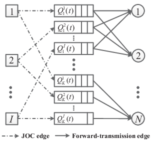
(3)

where $\mu_{k}^{i}(t)=\sum_{d_{n}^{t}:(s_{k,\textrm{b}}^{t},d_{n}^{t})\in\mathcal{E}_{t}^{\textrm{tr}}}y_{k,n}(t)w(s_{k,\textrm{b}}^{t},d_{n}^{t},i)$ captures the service process. Meanwhile, $A_{k}^{i}(t)=\varrho_{k}^{i}(t)x_{i,k}(t)B_{i,k}(t)$ models the equivalent traffic arrival process. We further denote $A_{i}(t)$ as the sum rate for flow $i$ at time slot $t$ , i.e., $A_{i}(t)=\sum_{k}A_{k}^{i}(t)$ . Besides, $Z^{+}=\max(0,Z)$ holds. In the following, we give a useful definition of queue stability.

Definition 1.

Queue $Q(t)$ is mean rate stable if $\underset{t\rightarrow\infty}{\lim}\frac{1}{t}\mathbb{E}[Q(t)]=0$ holds. A network of queues is stable if all the individual queues are mean rate stable.

According to the definition, we can gain the following two insights: 1) network stability is guaranteed if the length of all queues is finite; and 2) applying Little’s Theorem, we can depict average delay by queue length and further by queue stability for a stable queueing system.

Lemma 1.

Let queue $Q(t)$ be associated with stochastic arrival and service processes $A(t)$ and $u(t)$ . The time averages of both processes converge to $\overline{A}$ and $\overline{\mu}$ , respectively. The queue, $Q(t)$ , is mean rate stable if and only if $\overline{\mu}\geq\overline{A}$ holds.

The proof of Lemma 1 can be found in [33]. The intuition behind the lemma is that the network is stable if the traffic arrival can be served by the network in the long-term. As a result, the backlog of all queues is finite.

Theorem 1.

C1 can be approximately transformed into the mean rate queue stability constraint as $\textrm{C0}:\>\underset{t\rightarrow\infty}{\lim}\frac{1}{t}\mathbb{E}\left(|Q_{k}^{i}(t)|\right)=0\,\,\,\forall k,i.$

Proof:

Define $\overline{A_{k}^{i}}$ and $\overline{\mu_{k}^{i}}$ as

	$\displaystyle\overline{A_{k}^{i}}\triangleq\lim_{T\rightarrow\infty}\sum_{t=1}^{T}\frac{1}{T}\left(\varrho_{k}^{i}(t)x_{i,k}(t)B_{i,k}(t)\right)$		(4)
	$\displaystyle\overline{\mu_{k}^{i}}\triangleq\lim_{T\rightarrow\infty}\frac{1}{T}\sum_{t=1}^{T}\left(\sum_{d_{n}^{t}:(s_{k,\textrm{b}}^{t},d_{n}^{t})\in\mathcal{E}_{t}^{\textrm{tr}}}y_{k,n}(t)w(s_{k,\textrm{b}}^{t},d_{n}^{t},i)\right).$		(5)

For the flow conservation constraint in (1), summing over all time slots, dividing it by $T$ , and taking the limit, we obtain

		$\displaystyle\lim_{T\rightarrow\infty}\sum_{t=1}^{T}\frac{1}{T}\left(\varrho_{k}^{i}(t)x_{i,k}(t)B_{i,k}(t)+w(s_{k,\textrm{b}}^{t-1},s_{k,\textrm{b}}^{t},i)\right)$
	$\displaystyle=$	$\displaystyle\lim_{T\rightarrow\infty}\sum_{t=1}^{T}\frac{1}{T}\left(\sum_{d_{n}^{t}:(s_{k,\textrm{b}}^{t},d_{n}^{t})\in\mathcal{E}_{t}^{\textrm{tr}}}y_{k,n}(t)w(s_{k,\textrm{b}}^{t},d_{n}^{t},i)+w(s_{k,\textrm{b}}^{t},s_{k,\textrm{b}}^{t+1},i)\right).$			(6)

Recall that $w(s_{k,\textrm{b}}^{0},s_{k,\textrm{b}}^{1},i)=w(s_{k,\textrm{b}}^{T},s_{k,\textrm{b}}^{T+1},i)=0$ holds, it can thus be seen $\sum_{t=1}^{T}w(s_{k,\textrm{b}}^{t-1},s_{k,\textrm{b}}^{t},i)=\sum_{t=1}^{T}w(s_{k,\textrm{b}}^{t},s_{k,\textrm{b}}^{t+1},i)$ . Combining (4), (5) and (6), we obtain $\overline{A_{k}^{i}}=\overline{\mu_{k}^{i}}$ . Since our objective is to maximize a concave function of $A_{i}(t)$ , we can relax the above equation as $\overline{A_{k}^{i}}\leq\overline{\mu_{k}^{i}}$ without trading optimality. As a result, all queues in the network are mean rate stable, and C0 can be accordingly derived following Definition 1. ∎According to Theorem 1, problem (P1) can be reformulated as

	$\displaystyle(\textrm{P2})$	$\displaystyle\max_{\bm{X},\bm{Y},\bm{w},\bm{\varrho}}$	$\displaystyle\lim_{t\rightarrow\infty}\frac{1}{T}\sum_{t=1}^{T}\sum_{i=1}^{I}U_{i}(A_{i}(t))$
		$\displaystyle s.t.$	$\displaystyle\textrm{C0, C2-C10}.$

IV Proposed Solution and Performance Analysis

In this section, we first present an online algorithm, i.e., DMRC algorithm, to solve problem (P2). After that, we theoretically analyze its complexity as well as performance.

IV-A Dynamic Multi-Resource Cooperation Algorithm

We use the Lyapunov optimization theory [30, 34] to design an effective online algorithm to solve problem (P2). Firstly, we define a set of virtual queues $\bm{P}(t)=(P_{1}(t),P_{2}(t),\ldots,P_{I}(t))$ , with $P_{i}(t)$ being the virtual queue for flow $i$ . The virtual queue $P_{i}(t)$ evolves as

P_{i}(t+1)=[P_{i}(t)+p_{i}(t)]^{+}

(7)

where $p_{i}(t)=a_{i}-A_{i}(t)$ . When all virtual queues, $\bm{P}(t)$ , are stable, $\overline{p}_{i}\leq 0$ holds according to Lemma 1. Consequently, C7 is automatically satisfied. Let $\bm{\Theta}(t)=[\bm{Q}(t),\bm{P}(t)]$ be a concatenated vector of all actual and virtual queues and define the quadratic Lyapunov function as

L(\bm{\Theta}(t))=\frac{1}{2}\sum_{i=1}^{I}\sum_{k=1}^{K}Q_{k}^{i}(t)^{2}+\frac{1}{2}\sum_{i=1}^{I}P_{i}(t)^{2}.

(8)

Then, the one-slot conditional Lyapunov drift is given by

\Delta(\bm{\Theta}(t))=\mathbb{E}\{L(\bm{\Theta}(t+1))-L(\bm{\Theta}(t))|\bm{\Theta}(t)\}.

(9)

Lemma 2.

Assume $\bm{B}(t)$ and $\bm{C}(t)$ are independent identically distributed (i.i.d) over time slot $t$ . Under any feasible scheduling policy that satisfies all the constraints in problem (P1), we have the following inequality:

\Delta(\bm{\Theta}(t))-V\sum_{i}\mathbb{E}\left\{U_{i}(A_{i}(t))|\bm{\Theta}(t)\right\}\leq\Gamma-V\sum_{i=1}^{I}\mathbb{E}\left\{U_{i}(A_{i}(t))|\bm{\Theta}(t)\right\}\vskip-10.00002pt

+\sum_{i=1}^{I}\sum_{k=1}^{K}\mathbb{E}\left\{Q_{k}^{i}(t)(A_{k}^{i}(t)-\mu_{k}^{i}(t))|\bm{\Theta}(t)\right\}+\sum_{i=1}^{I}\mathbb{E}\left\{P_{i}(t)(a_{i}-A_{i}(t))|\bm{\Theta}(t)\right\}

(10)

where $V$ is a control factor to strike a balance between the queue backlog and the network utility, and $\Gamma$ is a finite constant that satisfies

\Gamma\geq\frac{1}{2}\sum_{i=1}^{I}\sum_{k=1}^{K}\{A_{k}^{i}(t)^{2}+\mu_{k}^{i}(t)^{2}\}+\frac{1}{2}\sum_{i=1}^{I}\{a_{i}-A_{i}(t)\}^{2}.

(11)

Proof:

See Appendix A. ∎The fundamental design philosophy of the proposed DMRC algorithm is to minimize the right-hand-side of (10) in each time slot. To be specific, firstly, at every time slot, observe the data queues $\bm{Q}(t)$ , virtual queues $\bm{P}(t)$ , and channel conditions $\bm{B}(t)$ and $\bm{C}(t)$ . Then, solve the following two subproblems in each time slot, namely Joint Observation Scheduling and Adaptive Processing (JOSAP) subproblem and Transmission Scheduling (TS) subproblem. A summary of DMRC algorithm is given in Algorithm 1.

Algorithm 1 Dynamic Multi-Resource Cooperation (DMRC) Algorithm

1: At each time slot, observe

\bm{Q}(t)

\bm{P}(t)

\bm{B}(t)

and

\bm{C}(t)

2: Obtain the observation scheduling decision

\bm{X}(t)

and compression ratio selection

\bm{\varrho}(t)

by solving the joint observation scheduling and adaptive processing subproblem (12):

		$\displaystyle\min_{\bm{X}(t),\bm{\varrho}(t)}\>$	$\displaystyle-V\sum_{i=1}^{I}U_{i}(A_{i}(t))+\sum_{i=1}^{I}\sum_{k=1}^{K}Q_{k}^{i}(t)A_{k}^{i}(t)-\sum_{i=1}^{I}P_{i}(t)A_{i}(t)$		(12)
		$\displaystyle s.t.$	$\displaystyle\textrm{C2},\textrm{C3},\textrm{C9},\textrm{C10}.$		(12)

3: Find transmission scheduling matrix

\bm{Y}(t)

by solving the transmission scheduling subproblem (13):

		$\displaystyle\max_{\bm{Y}(t)}\>$	$\displaystyle\sum_{i=1}^{I}\sum_{k=1}^{K}Q_{k}^{i}(t)\mu_{k}^{i}(t)$		(13)
		$\displaystyle s.t.$	$\displaystyle\textrm{C4},\textrm{C5},\textrm{C6},\textrm{C8}.$		(13)

4: Update

\bm{Q}(t)

and

\bm{P}(t)

according to (3) and (7), respectively.

IV-A1 Joint observation scheduling and adaptive processing subproblem

For the first subprobelm embedded in the proposed DMRC algorithm, a lemma is introduced to transform the objective function in (12).

Lemma 3.

Problem (12) can be equivalently transformed into the following problem, which is

			$\displaystyle\max_{\bm{X}(t),\bm{\varrho}(t)}\>V\sum_{i=1}^{I}\sum_{k=1}^{K}U_{i}(A_{k}^{i}(t))+\sum_{i=1}^{I}\sum_{k=1}^{K}Q_{k}^{i}(t)A_{k}^{i}(t)-\sum_{i=1}^{I}\sum_{k=1}^{K}P_{i}(t)A_{k}^{i}(t)$		(14)
		$\displaystyle s.t.$	$\displaystyle\textrm{C2},\textrm{C3},\textrm{C9},\textrm{C10}.$		(14)

Proof:

See Appendix B. ∎Observe that $A_{k}^{i}(t)=\varrho_{k}^{i}(t)x_{i,k}(t)B_{i,k}(t)$ is a nonlinear function in both $\varrho_{k}^{i}(t)$ and $x_{i,k}(t)$ in (14). To tackle this difficulty, we can view $A_{k}^{i}(t)$ as a separate decision variable for time slot $t$ and add corresponding constraints in the above optimization problem. This yields

	$\displaystyle\max_{\bm{X}(t),\bm{\varrho}(t),\bm{A}(t)}\>V\sum_{i=1}^{I}\sum_{k=1}^{K}U_{i}(A_{k}^{i}(t))+\sum_{i=1}^{I}\sum_{k=1}^{K}Q_{k}^{i}(t)A_{k}^{i}(t)-\sum_{i=1}^{I}\sum_{k=1}^{K}P_{i}(t)A_{k}^{i}(t)$	(15)
$\displaystyle s.t.$	$\displaystyle\textrm{C2},\textrm{C3},\textrm{C9},\textrm{C10}$
	$\displaystyle\textrm{C11}:\>A_{k}^{i}(t)\leq x_{i,k}(t)B_{i,k}(t)$
	$\displaystyle\textrm{C12}:\>A_{k}^{i}(t)\in\{0,\varrho_{1}B_{i,k}(t),...,\varrho_{J}B_{i,k}(t)\}.$

Note that $\varrho_{k}^{i}(t)$ is inherently captured in $A_{k}^{i}(t)$ . By relaxing discrete variables $x_{i,k}(t)$ and $A_{k}^{i}(t)$ into continuous ones, modified problem (15) turns into a convex optimization problem with a concave objective function and several linear inequalities constraints. The concavity of the objective function can be verified via calculating its second derivative in $A_{k}^{i}(t)$ . To solve this convex problem, we first give the partial Lagrangian of the primal problem (15) as

	$\displaystyle L(\bm{X}(t),\bm{A}(t),\bm{\alpha}(t))=V\sum_{i=1}^{I}\sum_{k=1}^{K}U_{i}(A_{k}^{i}(t))+\sum_{i=1}^{I}\sum_{k=1}^{K}Q_{k}^{i}(t)A_{k}^{i}(t)$	(16)
	$\displaystyle-\sum_{i=1}^{I}\sum_{k=1}^{K}P_{i}(t)A_{k}^{i}(t)+\sum_{i=1}^{I}\sum_{k=1}^{K}\alpha_{i,k}(t)\left(x_{k}^{i}(t)B_{i,k}(t)-A_{k}^{i}(t)\right)$
$\displaystyle s.t.$	$\displaystyle\textrm{C2},\textrm{C3},x_{i,k}(t)\in[0,1],A_{k}^{i}(t)\in[0,\varrho_{1}B_{i,k}(t)]$

where $\bm{\alpha}(t)=\{\alpha_{i,k}(t)\}$ are the set of dual variables corresponding to C11. We then rearrange the terms of (16) as follows:

	$\displaystyle L(\bm{X}(t),\bm{A}(t),\bm{\alpha}(t))=L_{1}(\bm{A}(t),\bm{\alpha}(t))+L_{2}(\bm{X}(t),\bm{\alpha}(t))$	(17)
	$\displaystyle=\sum_{i=1}^{I}\sum_{k=1}^{K}\left\{VU_{i}(A_{k}^{i}(t))+\left(Q_{k}^{i}(t)-P_{i}(t)-\alpha_{i,k}(t)\right)A_{k}^{i}(t)\right\}$	(17)
	$\displaystyle=+\alpha_{i,k}(t)\sum_{i=1}^{I}\sum_{k=1}^{K}\left(x_{k}^{i}(t)B_{i,k}(t)\right)$	(18)
$\displaystyle s.t.$	$\displaystyle\textrm{C2},\textrm{C3},x_{i,k}(t)\in[0,1],A_{k}^{i}(t)\in[0,\varrho_{1}B_{i,k}(t)].$	(19)

As such, if the optimal value of $\bm{\alpha}(t)$ is known, the dual objective function $L(\bm{X}(t),\bm{A}(t),\bm{\alpha}(t))$ is decomposed into two independent parts $L_{1}(\bm{A}(t),\bm{\alpha}(t))$ and $L_{2}(\bm{X}(t),\bm{\alpha}(t))$ , which correspond to (17) and (18), respectively. On the basis, problem (19) can be decomposed into the following two subproblems:

1) Compression Ratio Selection: The first one is the compression ratio selection problem as follows

	$\displaystyle\max_{\bm{A}(t)}\>L_{1}(\bm{A}(t),\bm{\alpha}(t))$
	$\displaystyle s.t.\>A_{k}^{i}(t)\in[0,\varrho_{1}B_{i,k}(t)].$		(20)

It can be solved using the standard optimization techniques and the KKT conditions [35]. As a result, we derive the optimal value $\left(A_{k}^{i}(t)\right)^{*}$ as

\left(A_{k}^{i}(t)\right)^{*}=\begin{cases}0,&\chi_{i,k}(t)\geq V\\ \varrho_{1}B_{i,k}(t),&\chi_{i,k}(t)\leq\frac{V}{1+\varrho_{1}B_{i,k}(t)}\\ \frac{V}{\chi_{i,k}(t)}-1,&\textrm{otherwise}\end{cases}

(21)

where $\chi_{i,k}(t)=\alpha_{i,k}(t)+P_{i}(t)-Q_{k}^{i}(t)$ . The concrete solving procedure can be found in Appendix C. From (21), we can get the optimal compression ratio $\left(\varrho_{k}^{i}(t)\right)^{*}$ by projecting $\left(A_{k}^{i}(t)\right)^{*}/B_{i,k}(t)$ into the set $\Lambda$ .

2) Observation Scheduling:

			$\displaystyle\max_{\bm{X}(t)}\>L_{2}(\bm{X}(t),\bm{\alpha}(t))$		(22)
		$\displaystyle s.t.$	$\displaystyle\textrm{C2},\textrm{C3},x_{i,k}(t)\in[0,1].$		(22)

In LP problem (22), all constraints are affine, and thus the feasible region is a polytope. According to [35], the optimal solution to an LP problem can only be achieved at the extreme point. In what follows, we give a lemma to show that each element within the optimal solution should be binary.

Lemma 4.

All elements $\{x_{i,k}^{*}(t)\}$ within the optimal solution to problem (22) are binary, i.e., $x_{i,k}^{*}(t)\in\{0,1\},\,\forall i,k$ .

Proof:

We prove the lemma by contradiction. The detailed procedure is similar to that in [36]. Assume that there exists at least an element $x_{\overline{i},\overline{k}}^{*}(t)$ within $\mathbf{x}=\{x_{i,k}^{*}(t)\}$ being non-binary, i.e., $0<x_{\overline{i},\overline{k}}^{*}(t)<1$ . On one hand, if constraints C2 and C3 are strict inequalities, we can construct two points $\mathbf{x}_{1}=\{\cdots,x_{\overline{i},\overline{k}}^{*}(t)+\epsilon,\cdots\}$ and $\mathbf{x}_{2}=\{\cdots,x_{\overline{i},\overline{k}}^{*}(t)-\epsilon,\cdots\}$ , wherein $(\cdots)$ indicates that other elements are the same with those in $\mathbf{x}$ , and $\epsilon$ is an arbitrarily small positive real number. As such, both $\mathbf{x}_{1}$ and $\mathbf{x}_{2}$ are within the polytope, and $0.5\mathbf{x}_{1}+0.5\mathbf{x}_{2}=\mathbf{x}$ holds. Hence, $\mathbf{x}$ is not an extreme point. On the other hand, if at least one constraint in C2 and C3 is tight, i.e., the equality holds, there must be another element $0<x_{\widehat{i,}\widehat{k}}^{*}(t)<1$ in $\mathbf{x}$ to guarantee the equality. Similarly, we can find two points $\mathbf{x}_{1}=\{\cdots,x_{\overline{i},\overline{k}}^{*}(t)+\epsilon,x_{\widehat{i,}\widehat{k}}^{*}(t)-\epsilon,\cdots\}$ and $\mathbf{x}_{2}=\{\cdots,x_{\overline{i},\overline{k}}^{*}(t)-\epsilon,x_{\widehat{i,}\widehat{k}}^{*}(t)+\epsilon\cdots\}$ within the polytope, such that $0.5\mathbf{x}_{1}+0.5\mathbf{x}_{2}=\mathbf{x}$ holds as well. This verifies that $\mathbf{x}$ is not an extreme point. To this end, Lemma 4 is proved. ∎From Lemma 4, we can equivalently transform problem (22) as

			$\displaystyle\max_{\bm{X}(t)}\>L_{2}(\bm{X}(t),\bm{\alpha}(t))$		(23)
		$\displaystyle s.t.$	$\displaystyle\textrm{C2},\textrm{C3},x_{i,k}(t)\in\{0,1\}.$		(23)

It can be seen that this problem is a weighted maximum matching problem as discussed in the following, where the weight can be set as corresponding observation link capacity. As a result, it can be solved optimally using existing algorithms. We should emphasize that the observation scheduling problem requires to be executed only once in each time slot, regardless of $\bm{\alpha}(t)$ in each iteration for solving the dual problem. This property greatly simplifies the solution procedure.

After solving the two subproblems, we need to iteratively update the Lagrange multipliers $\bm{\alpha}(t)$ . For this aim, a subgradient method can be used. More specifically, the $l$ -th update can be performed as

\alpha_{i,k}^{l+1}(t)=\left[\alpha_{i,k}^{l}(t)-\lambda_{l}(x_{k}^{i}(t)B_{i,k}(t)-A_{k}^{i}(t))\right]^{+}

(24)

where $\lambda_{l}$ is the sequence of scalar step sizes, and can be set as any square summable but not absolute summable value.

IV-A2 Transmission scheduling subproblem

Subproblem (13) can be reformulated into the following problem:

		$\displaystyle\max_{\bm{Y}(t)}\>$	$\displaystyle\sum_{k=1}^{K}\sum_{d_{n}^{t}:(s_{k,\textrm{b}}^{t},d_{n}^{t})\in\mathcal{E}_{t}^{\textrm{tr}}}Q_{k}^{i^{*}}(t)y_{k,n}(t)C_{k,n}(t)$		(25)
		$\displaystyle s.t.$	$\displaystyle\textrm{C4},\textrm{C5},\textrm{C8}$		(25)

where $i^{*}=\arg\max_{i}\,Q_{k}^{i},\,\forall k$ . Note that $w(s_{k,\textrm{b}}^{t},d_{n}^{t},i)$ in (25) is replaced by $C_{k,n}(t)$ since it is optimal to serve the flow with maximum transmission link capacity. To solve the reformulated problem, as shown in Fig. 5, we first utilize a bipartite graph to represent related components in the SIN. The vertices therein can be divided into two disjoint sets, i.e., the set of LEO satellites $\mathcal{K}$ and the set of destinations $\mathcal{N}$ . A destination $n$ is represented by $M_{n}$ vertices. Accordingly, link weight $W_{k,n}(t)$ is selected as the link capacity weighted queue backlog, $Q_{k}^{i^{*}}(t)C_{k,n}(t)$ . It can be observed that the formulated TS subproblem is identical to the maximum weighted matching problem in the constructed bipartite graph, and thereby efficient algorithms, e.g., Hungarian algorithm, can be applied to obtain the optimal solution.

IV-B Algorithm Analysis

Herein, we first analyze the computational complexity of the proposed DMRC algorithm. The complexity of the DMRC algorithm consists of two main parts: 2) JOSAP subproblem with the complexity of $O(\frac{1}{\epsilon}+I^{3})$ — It corresponds to complexity of compression ratio selection problem $O(\frac{1}{\epsilon})$ [37] and complexity of observation scheduling problem $O(I^{3})$ . For the compression ratio selection problem, the subgradient method converges to the desired state only after $O(\frac{1}{\epsilon})$ iterations, where $\epsilon$ is the maximum tolerance deviation from the optimal value. In each iteration, solving the problem only incurs $O(1)$ complexity, because a closed-form expression is available to the problem. As for the observation scheduling problem, it takes complexity of $O(I^{3})$ to solve the matching problem as described later. Thus, the complexity for solving JOSAP subproblem is $O(\frac{1}{\epsilon})+O(I^{3})$ ; 2) Transmission scheduling subproblem with the complexity of $O(K^{3})$ — This complexity comes from solving the maximum weighted matching problem on the constructed bipartite graph. It takes $O\left(\left(\max\{K,\sum_{n}M_{n}\}\right)^{3}\right)\approx O\left(K^{3}\right)$ for Hungarian algorithm to obtain the optimal solution [38]. Note that we make the approximation since the number of EOSs $K$ is generally larger than that of destinations $\sum_{n}M_{n}$ (i.e., virtual vertices corresponding to all destinations); Therefore, the overall computational complexity of DMRC algorithm can be derived as $O(\frac{1}{\epsilon}+I^{3}+K^{3})$ .

In parallel, we present the performance results of the DMRC algorithm. Specifically, the following theorem is given to characterize its asymptotic queue backlog and network utility.

Theorem 2.

The proposed DMRC algorithm yields the following time average queue backlog and network utility bounds:

\lim_{T\rightarrow\infty}\frac{1}{T}\sum_{t=1}^{T}\sum_{i=1}^{I}\sum_{k=1}^{K}\mathbb{E}\left\{Q_{k}^{i}(t)\right\}\leq\frac{\Gamma+VU^{*}}{\delta_{1}}\vskip-10.00002pt

(26)

\lim_{T\rightarrow\infty}\frac{1}{T}\sum_{t=1}^{T}\sum_{i=1}^{I}\mathbb{E}\left\{U_{i}(A_{i}(t))\right\}\geq U^{*}-\frac{\Gamma}{V}.

(27)

Proof:

See Appendix D. ∎It can be noticed that Theorem 1 proves the utility optimality of DMRC algorithm. Since Theorem 1 holds for all $V>0$ , we can choose a sufficiently large $V$ such that $\Gamma/V$ is arbitrarily small and the achieved utility of DMRC algorithm is arbitrarily close to optimal.

V Simulation Results

In this section, extensive experiments are conducted using Matlab simulator to evaluate the performance of our proposed DMRC algorithm. We present the simulation results from two aspects. First, we evaluate both the network utility and queue dynamics by changing the control factor, $V$ . Then, we investigate impacts of different network parameters on the DMRC performance.

We have conducted a set of simulations of SINs operating at the time horizon from 1 Jan. 2018 04:00:00 to 2 Jan. 2018 04:00:00. The time horizon is discretized into 1440 equal time slots, with the interval of each time slot being 60 seconds. Eight targets are located on the Earth’s surface, i.e., Mamiraua ( $2^{\circ}$ S, $66^{\circ}$ W), Cape York ( $11^{\circ}$ S, $142.5^{\circ}$ E), Alaska Coast ( $60^{\circ}$ N, $148^{\circ}$ W), Himalaya ( $28^{\circ}$ N, $87^{\circ}$ E), Sahara ( $28^{\circ}$ N, $11.5^{\circ}$ E), Sumatra ( $2^{\circ}$ S, $103^{\circ}$ E), Greenland ( $69^{\circ}$ N, $49^{\circ}$ W) and Bora ( $16^{\circ}$ S, $151^{\circ}$ W). Meanwhile, a number of LEO satellites are uniformly distributed over 2 sun-synchronous orbits at a height of 619.6km with inclination $97.86^{\circ}$ . We further set two relay satellites locating at nominal longitudes of $176.76^{\circ}$ E and $16.65^{\circ}$ E as the destinations. The set of available observation links and transmission links are obtained using the Satellite Tool Kit (STK) software. The observation link capacity is i.i.d. over time slots and randomly takes values from the set $\{600,800,1000\}$ Mbps, while the transmission link capacity is uniformly distributed in the set $\{0,200,400\}$ Mbps. The set of all compression ratio is assumed to be $\{\frac{2}{3},\frac{1}{2},\frac{1}{3},\frac{1}{4}\}.$

V-A Network Utility and Queue Dynamics

In Fig. 6, we evaluate the average network utility performance versus the value of control factor $V$ ranging from 1000 to 8000. Clearly, the average network utility increases with an increase of $V$ . However, the rate of network utility increases reduces with larger $V$ . This is because the network utility is a concave function of $V$ . We take a large value of $V$ to illustrate the optimal network utility ( $V=50000$ in our setting). We compare the network utility obtained by $V$ ranging from 1000 to 8000 to the network utility obtained by $V=50000$ . As shown in the figure, the increase of network utility from $V=8000$ to $V=50000$ is quite limited in comparison to the increasing from $V=1000$ to $V=8000$ . Therefore, the network utility achieved when $V=8000$ is close to the value of optimal network utility.

Fig. 7 shows the data queue occupancy for different values of $V$ . The time-average lengths of data queues increase with the value of $V$ . It can be seen that, with the increase of $V$ , the network utility of DMRC algorithm asymptotically approaches the optimality, which comes at a price of linearly growing average queue length. The observation confirms the correctness of Theorem 1. On the other hand, we further observe that both the average network throughput and queue backlog tend to increase with the growth in the number of transceivers $M_{n}=M$ , because more contacts can be established.

V-B Performance Comparison

We validate the efficiency of proposed DMRC algorithm by comparing it with two benchmark algorithms. The first one is random allocation algorithm (denoted as Random), wherein observation resource, transmission resource and compression ratio are randomly selected. The second one is named as Fixed-CR algorithm, wherein both the observation and transmission resources are allocated based on the maximum weighted matching method, and the compression ratio is fixed at $\frac{1}{4}$ . We set $V=8000$ and $M=2$ in the following simulations if not specified otherwise.

V-B1 The number of EOSs

In this experiment, we study the network performance of different algorithms versus the number of EOSs. The minimum rate requirement for an EOS is set to 0. Fig. 8 demonstrates that, with the increase of the number of EOSs, the average network utility improves for all the tested algorithms. As the number of EOSs grows, there are more observation resources and transmission resources. Therefore, each flow can get more chances to be served. It is observed that the DMRC algorithm achieves higher network utility than that of Random and Fixed-CR algorithms. The reason lies in that the DMRC algorithm tends to build high quality observation and transmission links. Also, the DMRC algorithm is able to adaptively select compression ratio to process the acquired image data.

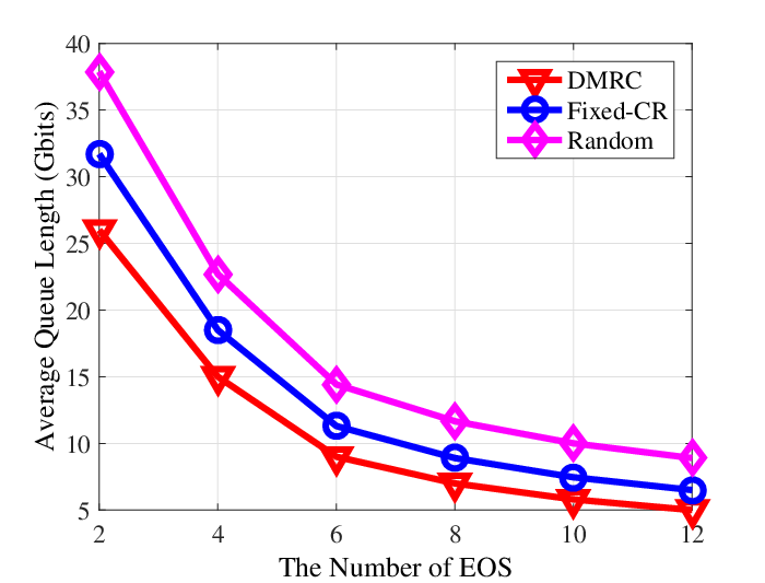
Fig. 9 presents the average queue length performance versus the number of EOSs. The average queue length decreases with the increasing number of EOSs, as more resources can be utilized to serve a flow. Besides, the DMRC algorithm yields the shortest queue length. This can be explained for two aspects. On one hand, the DMRC algorithm prefers to serve EOSs with longer queue length and adopts higher compression ratio to reduce queue backlog. On the other hand, through constructing high quality transmission links, the DMRC algorithm can deliver observation data more quickly. To validate the performance gain of the DMRC algorithm, we further plot the resource utilization ratio for different algorithms. As depicted in Fig. 10, the proposed DMRC algorithm has the highest utilization ratio of both the observation and transmission resources.

V-B2 Minimum data rate requirements

We evaluate the effects of minimum required data rate requirements on the network performance. In the following experiments, the number of EOSs is equal to 6. As illustrated in Fig. 11, with the minimum data rate varying from 0 to 60Mbps, the average network utility for the three algorithms follows a declining trend. This can be accounted by the fact that more resources are assigned to EOSs with poor channel quality to ensure their minimum data rate requirements. Hence, the network utility can be deteriorated to some extent. From Fig. 12, we observe that the average queue length becomes larger with the rise of minimum data rate requirement. The trend is expected, because given a higher data rate, the bottleneck EOSs need more resources to counteract undesired channel conditions. This reduces the efficiency in resource allocation. Another observation is that the DMRC algorithm achieves superior performance with respect to average network utility and queue backlog, in comparison with Random and Fixed-CR algorithms, for the reason similar to that stated before.

V-B3 The number of transceivers

In the following simulations, we investigate the performance impacts of the number of transceivers on destination relay satellites. The number of EOSs is 12, and the minimum date rate requirement is zero. Fig. 13 and Fig. 14 depict the average network utility and queue length performance for the three algorithms, respectively. With an increasing number of transceivers, the average network utility for DMRC, Random and Fixed-CR algorithms increases. We attribute the results to more available transmission resources, and thus more observation data can be transferred to destinations. Moreover, a smaller compression ratio can be chosen to yield higher image quality as well as network utility. However, as the number of transceivers further increases, both the average network utility and queue length remain steady. Under this circumstance, the observation resource turns to become the bottleneck, and thus additional transmission resource cannot be used for efficient data delivery.

VI Conclusion

In this paper, we have investigated the problem of multi-resource dynamic coordinate scheduling for SINs. Based on the Lyapunov optimization theory, a low complexity algorithm, i.e., the DMRC algorithm, is proposed to properly balance among the observation, computation and transmission resources. Extensive simulations have been conducted to verify that the newly proposed DMRC algorithm performs arbitrarily close to the optimal without requiring any prior knowledge. The impacts of various network parameters are evaluated on both the average network utility and queue backlog. There are a few open issues to be addressed for future studies. First, we intend to incorporate the reconfiguration delay into consideration when an EOS switches between two observation targets. Second, we aim to exploit the predictable network topology information to further reduce the queue backlog of the proposed DMRC algorithm. Last but not the least, how to effectively accommodate diverse QoS requirements, e.g., end-to-end delay and observing resolution requirements, should be studied.

Appendix A Proof of Lemma 2

According to the queue dynamics in (3), we have

$\displaystyle Q_{k}^{i}(t+1)^{2}-Q_{k}^{i}(t)^{2}$		(28)
	$\displaystyle=\{[Q_{k}^{i}(t)-\mu_{k}^{i}(t)]^{+}+A_{k}^{i}(t)\}^{2}-Q_{k}^{i}(t)^{2}$
	$\displaystyle=\{[Q_{k}^{i}(t)-\mu_{k}^{i}(t)]^{+}\}^{2}+2A_{k}^{i}(t)[Q_{k}^{i}(t)-\mu_{k}^{i}(t)]^{+}+A_{k}^{i}(t)^{2}-Q_{k}^{i}(t)^{2}$
	$\displaystyle\leq\{Q_{k}^{i}(t)-\mu_{k}^{i}(t)\}^{2}+2A_{k}^{i}(t)Q_{k}^{i}(t)+A_{k}^{i}(t)^{2}-Q_{k}^{i}(t)^{2}$
	$\displaystyle=A_{k}^{i}(t)^{2}+\mu_{k}^{i}(t)^{2}+2Q_{k}^{i}(t)\{A_{k}^{i}(t)-\mu_{k}^{i}(t)\}.$

Similarly, based on virtual queue formula (7), we further obtain

P_{i}(t+1)^{2}-P_{i}(t)^{2}\leq\{a_{i}-A_{i}(t)\}^{2}+2P_{i}(t)\{a_{i}-A_{i}(t)\}.

(29)

Considering the boundness property of $A_{k}^{i}(t)$ and $\mu_{k}^{i}(t)$ , we can always find a constant, $\Gamma$ , that satisfies

\Gamma\geq\frac{1}{2}\sum_{i=1}^{I}\sum_{k=1}^{K}\{A_{k}^{i}(t)^{2}+\mu_{k}^{i}(t)^{2}\}+\frac{1}{2}\sum_{i=1}^{I}\{a_{i}-A_{i}(t)\}^{2}.

(30)

Combining all the above three formulas, the following inequality holds

L(\bm{\Theta}(t+1))-L(\bm{\Theta}(t))\leq\Gamma+\sum_{i=1}^{I}\sum_{k=1}^{K}\left\{Q_{k}^{i}(t)(A_{k}^{i}(t)-\mu_{k}^{i}(t))\right\}+\sum_{i=1}^{I}\left\{P_{i}(t)(a_{i}-A_{i}(t))\right\}.

(31)

Adding $V\sum_{i=1}^{I}U_{i}(A_{i}(t))$ to both sides of the above inequation and taking conditional expectations yield (10). This completes the proof of Lemma 2.

Appendix B Proof of Lemma 3

By substituting $A_{i}(t)=\sum_{k}A_{k}^{i}(t)$ into the objective function, we have

	$\displaystyle\min\>-V\sum_{i=1}^{I}U_{i}(A_{i}(t))+\sum_{i=1}^{I}\sum_{k=1}^{K}Q_{k}^{i}(t)A_{k}^{i}(t)-\sum_{i=1}^{I}P_{i}(t)A_{i}(t)$
	$\displaystyle=\max\>V\sum_{i=1}^{I}U_{i}(\sum_{k=1}^{K}A_{k}^{i}(t))+\sum_{i=1}^{I}\sum_{k=1}^{K}Q_{k}^{i}(t)A_{k}^{i}(t)-\sum_{i=1}^{I}\sum_{k=1}^{K}P_{i}(t)A_{k}^{i}(t).$		(32)

Since $\sum_{k=1}^{K}x_{i,k}(t)\leq 1$ and $x_{i,k}(t)\in\{0,1\}$ holds, there is at most one $k^{*}\in\mathcal{K}$ for flow $i$ such that $x_{i,k^{*}}(t)=1$ ; Otherwise, $x_{i,k}(t)=0$ . By extension, there is at most one $k^{*}\in\mathcal{K}$ for flow $i$ such that $A_{i,k^{*}}(t)>0$ . To this end, we derive

V\sum_{i=1}^{I}U_{i}(\sum_{k=1}^{K}A_{k}^{i}(t))=V\sum_{i=1}^{I}U_{i}(A_{k^{*}}^{i}(t))=V\sum_{i=1}^{I}\sum_{k=1}^{K}U_{i}(A_{k}^{i}(t)).

(33)

By substituting (33) into (32), we obtain (14). This completes the proof of Lemma 3.

Appendix C Calculation of Optimal Arrival Rate

Recall that we set $U_{i}(A_{k}^{i}(t))=\log(1+A_{k}^{i}(t)),\>\forall k,i$ in this paper. Clearly, $U_{i}^{{}^{\prime}}(A_{k}^{i}(t))=\frac{1}{1+A_{k}^{i}(t)}$ . Subsequently, we can get the first derivative of $L_{1}(\bm{A}(t),\bm{\alpha}(t))$ with respect to $A_{k}^{i}(t)$ as

		$\displaystyle L_{1}^{{}^{\prime}}(\bm{A}(t),\bm{\alpha}(t))$	$\displaystyle=\frac{V}{1+A_{k}^{i}(t)}-\left(\alpha_{i,k}(t)+P_{i}(t)-Q_{k}^{i}(t)\right)$		(34)
			$\displaystyle=\frac{V}{1+A_{k}^{i}(t)}-\chi_{i,k}(t).$		(34)

1.

If $L_{1}^{{}^{\prime}}(\bm{A}(t),\bm{\alpha}(t))\leq 0$ holds for all $A_{k}^{i}(t)\in[0,\varrho_{1}B_{i,k}(t)]$ , the maximum value can be obtained at $A_{k}^{i}(t)=0$ , because $L_{1}(\bm{A}(t),\bm{\alpha}(t))$ is a monotone decreasing function in the considered interval. In this case, $\frac{V}{1+A_{k}^{i}(t)}-\chi_{i,k}(t)\leq 0$ is always satisfied within $[0,\varrho_{1}B_{i,k}(t)]$ , which means $\chi_{i,k}(t)\geqslant V$ .
2.

If $L_{1}^{{}^{\prime}}(\bm{A}(t),\bm{\alpha}(t))\geq 0$ holds for all $A_{k}^{i}(t)\in[0,\varrho_{1}B_{i,k}(t)]$ , we can see that $\chi_{i,k}(t)\leq\frac{V}{1+\varrho_{1}B_{i,k}(t)}$ . Since $L_{1}(\bm{A}(t),\bm{\alpha}(t))$ is a monotone increasing function, the optimality is achieved at $A_{k}^{i}(t)=\varrho_{1}B_{i,k}(t)$ .
3.

Otherwise, the optimal value is gained by setting $L_{1}^{{}^{\prime}}(\bm{A}(t),\bm{\alpha}(t))=0$ . This results in $A_{k}^{i}(t)=\frac{V}{\chi_{i,k}(t)}-1$ .

Summarizing the above cases, we finally attain the optimal solution $\left(A_{k}^{i}(t)\right)^{*}$ .

Appendix D Proof of Theorem 1

We prove the theorem by comparing the Lyapunov drift with a stationary and randomized algorithm denoted by $\Pi$ . An algorithm $\Pi$ makes a decision as a function of the observed state of the random events in each time slot. It is independent of the queue backlog information. According to the stochastic network optimization theory, given an arbitrarily small $\epsilon>0$ and constant positive scalars $\delta_{1}$ and $\delta_{2}$ , algorithm $\Pi$ can yield

\mathbb{E}\left\{U_{i}(\widetilde{A}_{i}(t))\right\}\leq U^{*}+\epsilon\vskip-15.00002pt

(35)

\mathbb{E}\left\{\widetilde{A}_{k}^{i}(t)-\widetilde{\mu}_{k}^{i}(t)\right\}\leq\delta_{1}\vskip-15.00002pt

(36)

\mathbb{E}\left\{a_{i}-\widetilde{A}_{i}(t)\right\}\leq\delta_{2}

(37)

where $\widetilde{A}_{k}^{i}(t)$ and $\widetilde{\mu}_{k}^{i}(t)$ are corresponding variables generated by algorithm $\Pi$ . Since the DMRC algorithm minimizes the right-hand-side of (10), we have

\Delta(\bm{\Theta}(t))-V\sum_{i}\mathbb{E}\left\{U_{i}(A_{i}(t))|\bm{\Theta}(t)\right\}\leq\Gamma-V\sum_{i=1}^{I}\mathbb{E}\left\{U_{i}(\widetilde{A}_{i}(t))|\bm{\Theta}(t)\right\}\vskip-15.00002pt

+\sum_{i=1}^{I}\sum_{k=1}^{K}\mathbb{E}\left\{Q_{k}^{i}(t)(\widetilde{A}_{k}^{i}(t)-\widetilde{\mu}_{k}^{i}(t))|\bm{\Theta}(t)\right\}+\sum_{i=1}^{I}\mathbb{E}\left\{P_{i}(t)(a_{i}-\widetilde{A}_{i}(t))|\bm{\Theta}(t)\right\}.

(38)

Substituting (35)–(37) into (38), we get the following inequation as $\epsilon\rightarrow 0$

\Delta(\bm{\Theta}(t))-V\sum_{i}\mathbb{E}\left\{U_{i}(A_{i}(t))|\bm{\Theta}(t)\right\}\leq\Gamma-VU^{*}+\delta_{1}\sum_{i=1}^{I}\sum_{k=1}^{K}\mathbb{E}\left\{Q_{k}^{i}(t)\right\}.

(39)

Taking iterated expectation of (39) over $t\in\{1,...,T-1,T\}$ and using the law of telescoping sums result in

\mathbb{E}\left\{L(\bm{\Theta}(T))\right\}-\mathbb{E}\left\{L(\bm{\Theta}(0))\right\}-V\sum_{t=1}^{T}\sum_{i=1}^{I}\mathbb{E}\left\{U_{i}(A_{i}(t))\right\}\vskip-15.00002pt

\leq T\left(\Gamma-VU^{*}\right)+\delta_{1}\sum_{t=1}^{T}\sum_{i=1}^{I}\sum_{k=1}^{K}\mathbb{E}\left\{Q_{k}^{i}(t)\right\}.

Reducing the left-hand-side, increasing its right-hand-side by eliminating all negative terms, and then rearranging it, we get

\lim_{T\rightarrow\infty}\frac{1}{T}\sum_{t=1}^{T}\sum_{i=1}^{I}\sum_{k=1}^{K}\mathbb{E}\left\{Q_{k}^{i}(t)\right\}\leq\frac{\Gamma+VU^{*}}{\delta_{1}}.

Similarly, we can obtain

\lim_{T\rightarrow\infty}\frac{1}{T}\sum_{t=1}^{T}\sum_{i=1}^{I}\mathbb{E}\left\{U_{i}(A_{i}(t))\right\}\geq U^{*}-\frac{\Gamma}{V}.

References

[1] G. Wu, W. Pedrycz, H. Li, M. Ma, and J. Liu, “Coordinated planning of heterogeneous earth observation resources,” IEEE Trans. Syst., Man, Cybern: Syst., vol. 46, no. 1, pp. 109–124, Jan. 2016.
[2] M. D. Sanctis, E. Cianca, G. Araniti, I. Bisio, and R. Prasad, “Satellite communications supporting internet of remote things,” IEEE Internet of Things Journal, vol. 3, no. 1, pp. 113–123, Feb. 2016.
[3] M. Shimada, T. Tadono, and A. Rosenqvist, “Advanced land observing satellite (ALOS) and monitoring global environmental change,” Proceedings of the IEEE, vol. 98, no. 5, pp. 780–799, May 2010.
[4] M. Chi, A. Plaza, J. A. Benediktsson, Z. Sun, J. Shen, and Y. Zhu, “Big data for remote sensing: challenges and opportunities,” Proceedings of the IEEE, vol. 104, no. 11, pp. 2207–2219, Nov. 2016.
[5] M. Sheng, Y. Wang, J. Li, R. Liu, D. Zhou, and L. He, “Toward a flexible and reconfigurable broadband satellite network: resource management architecture and strategies,” IEEE Wireless Commu., vol. 24, no. 4, pp. 127–133, Aug. 2017.
[6] C. Jiang, X. Wang, J. Wang, H.-H. Chen, and Y. Ren, “Security in space information networks,” IEEE Commun. Mag., vol. 53, no. 8, pp. 82–88, Aug. 2015.
[7] J. Du, C. Jiang, M. Guizani, and Y. Ren, “Cooperative earth observation through complex space information networks,” IEEE Wireless Commu., vol. 23, no. 2, pp. 136–144, Apr. 2016.
[8] Q. Yu, W. Meng, M. Yang, L. Zheng, and Z. Zhang, “Virtual multi-beamforming for distributed satellite clusters in space information networks,” IEEE Wireless Commu., vol. 23, no. 1, pp. 95–101, Feb. 2016.
[9] N. Zhang, S. Zhang, P. Yang, O. Alhussein, W. Zhuang, and X. Shen, “Software defined space-air-ground integrated vehicular networks: challenges and solutions,” IEEE Commu. Mag., vol. 55, no. 7, pp. 101–109, Jul. 2017.
[10] J. Du, C. Jiang, Y. Qian, Z. Han, and Y. Ren, “Resource allocation with video traffic prediction in cloud-based space systems,” IEEE Trans. Multimedia, vol. 18, no. 5, pp. 820–830, May 2016.
[11] Y. Wang, M. Sheng, W. Zhuang, S. Zhang, N. Zhang, R. Liu, and J. Li, “Multi-resource coordinate scheduling for earth observation in space information networks,” IEEE J. Sel. Areas Commun., vol. 36, no. 2, pp. 268–279, Feb. 2018.
[12] N. Bianchessi and G. Righini, “Planning and scheduling algorithms for the COSMO-SkyMed constellation,” Aerospace Science and Technology, vol. 12, pp. 535–544, 2008.
[13] H. Chen, J. Wu, W. Shi, J. Li, and Z. Zhong, “Coordinate scheduling approach for EDS observation tasks and data transmission jobs,” Journal of Systems Engineering and Electronics, vol. 27, no. 4, pp. 822–835, Aug. 2016.
[14] R. Liu, M. Sheng, K.-S. Lui, X. Wang, Y. Wang, and D. Zhou, “An analytical framework for resource-limited small satellite networks,” IEEE Commu. Letters, vol. 20, no. 2, pp. 388–391, Feb. 2016.
[15] D. Zhou, M. Sheng, X. Wang, C. Xu, R. Liu, and J. Li, “Mission aware contact plan design in resource-limited small satellite networks,” IEEE Trans. Commu., vol. 65, no. 6, pp. 2451–2466, Jun. 2017.
[16] D. Y. Liao and Y. T. Yang, “Imaging order scheduling of an earth observation satellite,” IEEE Trans. Syst., Man, Cybern. C, Appl. Rev., vol. 37, no. 5, pp. 794–802, Sep. 2007.
[17] A. D. Panagopoulos, P. M. Arapoglou, and P. G. Cottis, “Satellite communications at Ku, Ka and V bands, propagation impairments and mitigation techniques,” IEEE Commu. Surveys & Tutorials, vol. 6, no. 3, pp. 2–14, Oct. 2004.
[18] Y. Wang, M. Sheng, J. Li, X. Wang, R. Liu, and D. Zhou, “Dynamic contact plan design in broadband satellite networks with varying contact capacity,” IEEE Commu. Letters, vol. 20, no. 16, pp. 2410–2413, Dec. 2016.
[19] K. Kaneko, Y. Kawamoto, H. Nishiyama, N. Kato, and M. Toyoshima, “An efficient utilization of intermittent surface-satellite optical links by using mass storage device embedded in satellites,” Performance Evaluation, vol. 87, pp. 37–46, May 2015.
[20] H. Nishiyama, Y. Tada, N. Kato, N. Yoshimura, M. Toyoshima, and N. Kadowaki, “Toward optimized traffic distribution for efficient network capacity utilization in two-layered satellite networks,” IEEE Transactions on Vehicular Technology, vol. 62, no. 3, pp. 1303–1313, March 2013.
[21] D. Fischer, D. Basin, K. Eckstein, and T. Engel, “Predictable mobile routing for spacecraft networks,” IEEE Transactions on Mobile Computing, vol. 12, no. 6, pp. 1174–1187, June 2013.
[22] B. Deng, C. Jiang, L. Kuang, S. Guo, J. Lu, and S. Zhao, “Two-phase task scheduling in data relay satellite systems,” IEEE Trans. Veh. Technol., vol. 67, no. 2, pp. 1782–1793, Oct. 2017.
[23] X. Jia, T. Lv, F. He, and H. Huang, “Collaborative data downloading by using inter-satellite links in LEO satellite networks,” IEEE Trans. Wireless Commu., vol. 16, no. 3, pp. 1523–1532, Mar. 2017.
[24] J. A. Fraire and J. M. Finochietto, “Design challenges in contact plans for disruption-tolerant satellite networks,” IEEE Commun. Mag., vol. 53, no. 5, pp. 163–169, May 2015.
[25] J. Du, C. Jiang, J. Wang, Y. Ren, S. Yu, and Z. Han, “Resource allocation in space multiaccess systems,” IEEE Trans. Aerosp. Electron., vol. 53, no. 2, pp. 598–618, Apr. 2017.
[26] F. Li, S. Chen, M. Huang, Z. Yin, C. Zhang, and Y. Wang, “Reliable topology design in time-evolving delay-tolerant networks with unreliable links,” IEEE Trans. Mobile Computing, vol. 14, no. 6, pp. 1301–1314, June 2015.
[27] S. Merugu, M. Ammar, and E. Zegura, “Routing in space and time in networks with predictable mobility,” GIT, Tech. Rep. CC-04-07, 2004.
[28] M. Azimifar, T. D. Todd, A. Khezrian, and G. Karakostas, “Vehicle-to-vehicle forwarding in green roadside infrastructure,” IEEE Trans. Veh. Technol., vol. 65, no. 2, pp. 780–795, Feb. 2016.
[29] D. Zhang, Z. Chen, M. K. Awad, N. Zhang, H. Zhou, and X. S. Shen, “Utility-optimal resource management and allocation algorithm for energy harvesting cognitive radio sensor networks,” IEEE J. Sel. Areas Commun., vol. 34, no. 12, pp. 3552–3565, Dec. 2016.
[30] H. Xiong, R. Li, A. Eryilmaz, and E. Ekici, “Delay-aware cross-layer design for network utility maximization in multi-hop networks,” IEEE J. Sel. Areas Commun., vol. 29, no. 5, pp. 951–959, May 2011.
[31] V. V. Vazirani, Approximation algorithms. Springer Science & Business Media, 2013.
[32] G. Konidaris, S. Toumpis, and S. Gitzenis, “Primal decomposition and online algorithms for flow optimization in wireless DTNs,” in Proc. IEEE GLOBECOM, Dec 2013, pp. 84–90.
[33] M. J. Neely, Stochastic Network Optimization with Application to Communication and Queueing Systems. San Rafael, CA, USA: Morgan & Claypool, 2010.
[34] M. J. Neely, E. Modiano, and C. E. Rohrs, “Power allocation and routing in multi-beam satellites with time varying channels,” IEEE Trans. Netw., vol. 11, no. 1, pp. 138–152, Feb. 2003.
[35] S. Boyd and L. Vandenberghe, Convex Optimization. New York, NY, USA: Cambridge Univ. Press, 2004.
[36] D. Zhai, M. Sheng, X. Wang, Y. Li, J. Song, and J. Li, “Rate and energy maximization in scma networks with wireless information and power transfer,” IEEE Commu. Letters, vol. 20, no. 2, pp. 360–363, Feb. 2016.
[37] W. Yu and R. Lui, “Dual methods for nonconvex spectrum optimization of multicarrier systems,” IEEE Trans. Commun., vol. 54, no. 7, pp. 1310–1322, Jul. 2006.
[38] H. W. Kuhn, “The Hungarian method for the assignment problem,” Naval Res. Logistics Quart., vol. 2, no. 1-2, pp. 83–97, Mar. 1955.