A new and consistent well model for one-phase flow in anisotropic porous media using a distributed source model

In the following section, we derive an analytical solution for one-phase flow around an infinite cylindrical well $\Gamma$ with radius $r_{\omega}$ in an infinite porous domain $\hat{\Omega}=\mathbb{R}^{3}\setminus\Gamma$ with anisotropic, homogeneous permeability. We assume, without loss of generality, that the well axis passes through the origin of the Cartesian coordinate system, and denote by $\boldsymbol{\psi}$ a unit vector parallel to the well signifying the well orientation. We seek an analytical expression for the hydraulic pressure $p$ such that

for a constant well pressure $p_{\omega}$ in $\mathrm{Pa}$ and some specific pumping rate $q$ in $\mathrm{kg}\text{\,}{\mathrm{s}}^{-1}\text{\,}{\mathrm{m}}^{-1}$ given on $\partial\Gamma$. The total mass flow over the boundary of a well segment of length $L$ is thus given by $Q=qL$.

From thermodynamic constraints, $K$ is a positive definite and symmetric, second-order tensor field. Hence, $K$ can be decomposed such that

where $D=\operatorname{diag}(\lambda_{1},\lambda_{2},\lambda_{3})$ is a diagonal matrix composed of the eigenvalues $\lambda_{i}$ of $K$, $Q=[\boldsymbol{\nu}_{K,1}|\boldsymbol{\nu}_{K,2}|\boldsymbol{\nu}_{K,3}]$ is a rotation matrix with the corresponding eigenvectors as columns, and $A^{T}$ denotes the transpose of a matrix $A$. Further useful properties derived from the decomposition are $\operatorname{det}(K)=\lambda_{1}\lambda_{2}\lambda_{3}$, where $\operatorname{det}(A)$ denotes the determinant of $A$, and $K^{n}=Q\Lambda^{n}Q^{T}$, where $D^{r}=\operatorname{diag}({\lambda_{1}^{r},\lambda_{2}^{r},\lambda_{3}^{r}})$, $r\in\mathbb{R}$.

It is well known that the anisotropic one-phase flow problem can be transformed to an isotropic problem using a coordinate transformation [9, 16, 17, 6, 18]

with the stretching matrix $\tilde{S}=k_{I}^{1/2}K^{-1/2}$, where $k_{I}$ is an arbitrary scalar constant, that we choose as $k_{I}=\operatorname{det}(K)^{-1/3}$ (cf. [9]), rendering the transformation isochoric. The transformation $\boldsymbol{u}=\tilde{S}\boldsymbol{x}$ deforms the well cylinder such that a cross-section orthogonal to the transformed well direction is elliptical. The solution to the isotropic problem

is identical on two parallel planes perpendicular to the transformed (normalized) well direction, $\boldsymbol{\psi}^{\prime}=\tilde{S}\boldsymbol{\psi}||\tilde{S}\boldsymbol{\psi}||^{-1}$. This motivates the rotation of the coordinate system such that the first and second axis are aligned with the major and minor axis of the well-bore ellipse and third axis is aligned with $\boldsymbol{\psi}^{\prime}$. To determine the corresponding rotation matrix $\tilde{R}$, we need to characterize this well-bore ellipse. The well cylinder in $x$-coordinates is given by

After stretching, the coordinate system can be rotated with the rotation matrix $R$ so that the third axis is aligned with the well direction. Then, projecting into the plane perpendicular to the well direction yields the well-bore ellipse equation

in $\hat{v}$-coordinates, where

The rotation matrix $R$ can be derived using Rodrigues’ rotation formula as shown in Appendix A. The length of the major and minor ellipse axis are found as $a=r_{w}\gamma_{1}^{-1/2}$ and $b=r_{w}\gamma_{2}^{-1/2}$, where $\gamma_{i}$ are the eigenvalues of $E$, and the axis orientations are given by $\boldsymbol{\nu}_{1}=P\hat{\boldsymbol{\nu}}_{E,1}$, $\boldsymbol{\nu}_{2}=P\hat{\boldsymbol{\nu}}_{E,2}$, where $\hat{\boldsymbol{\nu}}_{E,i}$ denote the corresponding eigenvectors of $E$. We assume that the eigenvalues and eigenvectors are sorted such that $a\geq b$, and oriented such that $\boldsymbol{\psi^{\prime}}=\boldsymbol{\nu}_{1}\times\boldsymbol{\nu}_{2}$. Finally the desired rotation is given by

where

is rotating about the well direction axis such that the coordinate system is aligned with the principal ellipse axes.

Following the derivations from above, we now have to solve a two-dimensional isotropic Laplace problem with boundary conditions prescribed on an ellipse. To this end, we note that the transformation of a harmonic function $f$ (a function satisfying Laplace’s equation $\Delta f=\nabla\cdot\!\nabla\!f=0$) with a conformal (angle-preserving) mapping yields another harmonic function [19] (see Appendix B). Using a Joukowsky transformation, a conformal mapping well-known from aerodynamics [20], the isotropic problem with a well with elliptic cross-sections, can be transformed to an isotropic problem with circular cross-sections [16]. Transforming into the complex plane (parametrizing the well-bore ellipse plane)

the (inverse) Joukowsky transformation

transforms elliptic isobars into circular isobars, where $a$ and $b$, $a\geq b$, are the major and minor axis of the well-bore ellipse, as derived above. In particular, the well-bore ellipse (where $p=p_{\omega}$) is mapped onto a circle with radius $r_{\circ}=a+b$. Finally, in the new coordinate system we find the (now) radially symmetric analytical solution to problem Eq. 3.1

where the source scaling factor $\zeta$ is necessary to recover the original source $q$ on $\partial\Gamma$. This can be derived from simple geometric considerations as shown in Appendix C. The $w$ corresponding to some $x\in\hat{\Omega}$ in original coordinates is obtained by using all above-mentioned transformations after each other as follows

Such a solution for a slanted well ($30\text{\,}\mathrm{\SIUnitSymbolDegree}$ with respect to vertical axis) and anisotropic permeability tensor

is visualized in Fig. 2.

To construct a suitable kernel function for anisotropic problems, we first have a closer look at the properties of the employed Joukowsky transformation. The effect of the mapping $T$, Eq. 3.11, is shown in Fig. 3. Points on the exterior of a line on the real axis between $f$ and $-f$ are mapped onto the exterior of a circle with radius $f$. The ellipse with major axis $a$ and minor axis $b$ is mapped onto a circle with radius $r_{\circ}=a+b$. Going further away from the well, the deformation due to the mapping is less and less pronounced. This matches the expectations for the physical flow problem, since isobars at large distance from an elliptical well-bore become increasingly circular in isotropic media.

The inverse transformation is given by

where the restriction on $|w|$ is necessary to obtain a one-to-one mapping. The transformation $T^{-1}$ can equally be interpreted as an $\mathbb{R}^{2}\rightarrow\mathbb{R}^{2}$ mapping. The Jacobian of the transformation $T^{-1}$ for $z=x+iy$ and $w=u+iv$ has the form

which follows from the the Cauchy–Riemann equations [21]. Since the transformation can be viewed as the composition of a scaling and a rotation, it is angle-preserving. The transformation is associated with a spatially dependent volume deformation characterized by the determinant of $J_{T^{-1}}$. Furthermore, it can be shown that the Laplace operator behaves as follows under the transformation $z=T^{-1}(w)$,

by computing the derivative of the real and the imaginary part of $p$ separately, applying the chain rule and the Cauchy–Riemann equations, as shown for completeness in Appendix B. From Eq. 3.17 follows that

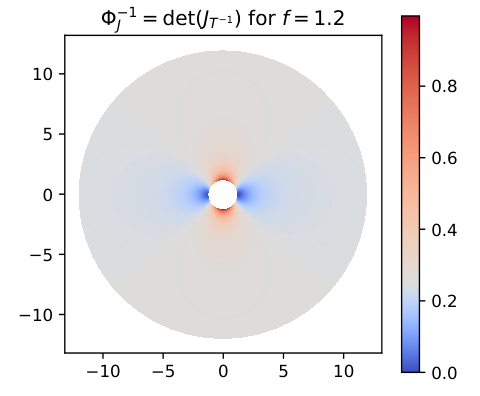
for the transformation $w=T(z)$. The determinant can be explicitly computed, using Eq. 3.17 and complex differentiation (shown in Appendix D) as

where $\Re(w^{2})$ is real part of $w^{2}$, and $|w|$ the absolute value of $w$. We note that $\Phi_{J}$ quickly converges to the value $4$ with increasing $|w|$, that is with increasing distance from the well. The function $\Phi_{J}^{-1}$ is plotted in Fig. 4 exemplarily for $f=1.2$.

Instead of excluding the well domain $\Gamma$ from $\Omega=\mathbb{R}^{3}$ and modeling infiltration or extraction by a flux boundary condition, we will now model the action of the well on the flow field by a spatially distributed source term, as presented for the isotropic problem,

From the above derivations, we know that solving Eq. 3.20 in $w$-coordinates is straight-forward. Hence, we choose kernel functions in $w$-coordinates and then transform to $x$-coordinates so that the pressure solution satisfies Eq. 3.20. Motivated by the properties of the Joukowsky transform (see Fig. 3), we choose a local kernel that is constant on the annulus with inner radius $f<\varrho_{i}\leq r_{\circ}$ and outer radius $\varrho_{o}>r_{\circ}$,

In $w$-coordinates, we can find a solution to the problem

for a given constant well pressure $p_{\omega}$, $\hat{q}=q\zeta$ and constant density and viscosity.

By means of integration (cf. [15]), we get

where $\xi^{2}=\varrho_{o}^{2}-\varrho_{i}^{2}$. This shows that outside the kernel support region ($|w|>\varrho_{o}$), we obtain the exact analytical solution derived in Section 3.1. Moreover, the source term can be reformulated, cf. [15],

where $p_{0}:=p(|w|=0)=p(|w|=\varrho_{i})$ is the fluid pressure evaluated on the well center-line. Note that for $f=0$ and $\varrho_{i}=f=0$, the isotropic solution with for a circular constant kernel (Eqs. 2.7 and 2.10) is obtained. From the transformation of the Laplace operator, Eq. 3.18, we see that the problem

with altered kernel function $\Phi_{\Lambda}=\Phi_{A}\Phi_{J}$ is equivalent to Eq. 3.22.

The transformation $T^{-1}$ changes shape of the kernel support $\mathcal{S}(\Phi_{A})$ from an annulus to an ellipse $E_{\Phi,v}$. Inverting $Z$ extrudes the solution along the well center-line, and inverting the rotation and stretch described by $V$ and $U$ results in a kernel support region in the shape of an elliptic cylinder. Moreover, each ellipse $E_{\Phi,v}$ with normal vector $\boldsymbol{e}_{3}$ is transformed to an ellipse $E_{\Phi,x}(s)$, that is the intersection the elliptic cylinder with a plane with the normal vector $\boldsymbol{n}_{E_{x}}=\tilde{S}\tilde{R}^{T}\boldsymbol{e}_{3}$, centered at $s$ on the well center-line. The transformation and the normal vector $\boldsymbol{n}_{E_{x}}$ are visualized in Fig. 5. We note that if none of the principal axes of the permeability tensor are aligned with the well direction, $\boldsymbol{n}_{E_{x}}$ is not parallel to the well direction $\boldsymbol{\psi}$ in $x$-coordinates. The integral of the right-hand side of Eq. 3.20 for a well segment $\Lambda_{i}$ with length $L_{i}$ is equal to the integral over the kernel support $\mathcal{S}(\Phi_{\Lambda,i})$ which has the shape of the elliptic cylinder given by

Using $\hat{q}=q\zeta$, and exploiting that $k_{I}$ was chosen such that $\operatorname{det}(\tilde{R}\tilde{S})=1$, it can be shown that

where $0\leq\hat{s}\leq\hat{L}_{i}$ is a local coordinate along the transformed well direction, and the last equality is proven in Appendix C. This is the desired property of the kernel function for the anisotropic case corresponding to Eq. 2.2 for the isotropic case.

The kernel integral in Eq. 4.3

is not easily approximated with a quadrature rule, since the intersection $K_{\Omega}\cap\mathcal{S}(\Phi_{\Lambda,\mathcal{I}})$, that is the intersection of an elliptic cylinder with for example a hexahedron is difficult to compute. However, we use the same idea as in [15], and remark that the integral over the entire support $\mathcal{S}(\Phi_{\Lambda,\mathcal{I}})$ is known exactly; see Eq. 3.27. Hence, the integration problem can be reformulated as the distribution of the known integral over all intersected control volumes $K_{\Omega}$ weighted with the respective support volume fractions. Following [15], we create $n_{\mathcal{I}}$ integration points $\boldsymbol{x}_{i}\in\mathcal{S}(\Phi_{\Lambda,\mathcal{I}})$ with known volume elements $V_{i}$ of similar size and shape, so that

Computing the weights for each cell $K_{\Omega}$ is a pre-processing step that only has to be done once for each computational mesh and well geometry.

In the first numerical experiment grid convergence is investigated for different anisotropy ratios $\alpha$. To this end, $h_{\text{max}}:=\operatorname{max}\limits_{K_{\Omega}\in\Omega_{h}}h_{K_{\Omega}}$, where $h_{K_{\Omega}}$ is defined as the maximum distance between two vertices of the cell $K_{\Omega}$. Starting at a grid resolution for $\Omega_{h}$ of $20\times 20\times 10$ cells ($h_{\text{max}}=10\sqrt{3}~$\mathrm{m}$$), the grid is refined uniformly. Figure 7 shows the errors $E_{p}$ and $E_{q}$ for different grid resolutions and values of $\alpha$, for $\beta_{1}=\beta_{2}=20^{\circ}$ and $\gamma_{1}=\gamma_{2}=-20^{\circ}$, so that $K$ is a full tensor and none of the principal axis of $K$ is aligned with the well direction. For all $\alpha$, the method shows second order convergence for the pressure in the given norm, as expected for the MPFA-O method [26] (super convergence at cell centers). The source term $q$ is a linear function of the pressure $p$ and also exhibits second order convergence. We note that the errors for different $\alpha$ are not directly comparable since the analytical solution for $p$ changes with $\alpha$, although $q$ is constant.

However, the convergence rates are shown to be independent of $\alpha$ with increasing grid resolution. The convergence rates for $E_{q}$ (slope of the lines in Fig. 7) are presented in Table 1. It can be seen that rates for large grid cells and large $\alpha$ are slightly smaller. This is because the kernel support is still under-resolved by the computational grid. For example, for $\alpha=100$, the kernel ellipse in $x$-coordinates has major and minor axis of $a_{x}\approx$55.9\text{\,}\mathrm{m}$$, $b_{x}\approx$5.6\text{\,}\mathrm{m}$$, respectively, while $h_{\text{max}}\approx$17.32\text{\,}\mathrm{m}$$ for the lowest grid resolution.

In [15], it is suggested that increasing the kernel support region (increasing $\varrho_{o}$), has a similar effect on $E_{q}$ as refining the grid. However, the pressure solution is then regularized in a larger region, so that there is a trade-off between the accuracy of the source term and the accuracy of the pressure field with respect to the unmodified problem ($\varrho_{o}\rightarrow\varrho_{i},\Phi_{\Lambda}\rightarrow\delta_{\Lambda}$). However, every discrete cell $K_{\Omega}$ can be also interpreted as a kernel support region, such that the choice of $\Phi_{\Lambda}$ enables us to better control the discretization error as soon as $\mathcal{S}(\Phi_{\Lambda},\mathcal{I})$ becomes larger than $K_{\Omega}$.

As shown in [6] and Fig. 4, isobars become circular, in the transformed domain $U(\Omega)$, with increasing distance to the well. Therefore, a reasonable simplification is $\Phi_{J}\approx 4$ if $\varrho_{o}\gg r_{\omega}$. This is completely analogous to the assumption of circular isobars in [6], where an estimate of the error introduced by the assumptions is given for the two-dimensional case.

In the following numerical experiment, we step-wise increase the kernel radius $\varrho_{o}$, for the same $20\times 20\times 10$ grid. This is done once for the case, where $\varrho_{o}\gg r_{\omega}$ and for the case for which $\varrho_{o}$ is only slightly larger than $r_{\omega}$. Furthermore, $\beta_{1}=\beta_{2}=20^{\circ}$ and $\gamma_{1}=\gamma_{2}=-20^{\circ}$. The results are shown in Fig. 8. First, it can be seen that doubling $\varrho_{o}$ leads to a $4$-times smaller error $E_{q}$. This can be explained by the fact that the larger the kernel, the more grid cells resolve the kernel support, and the better is the approximation of $p_{0}$. Furthermore, the result is consistent with the results in [15]. Moreover, Fig. 8 suggests that for $\varrho_{o}\gg r_{\omega}$ the simplification of the kernel function ($\Phi_{J}\approx 4$) is not visible in $E_{q}$, while for kernel radii slightly smaller than the well radius, the simplification increases $E_{q}$ by an order of magnitude in comparison to the case using the exact kernel function as derived in Section 3.3. The results show that the presented method is also applicable in cases where the grid resolution is very close to the well radius. An adaption of the presented method for other applications, such as the simulation of flow in vascularized tissue, where such ratios of vessel radius to cell size are typical, cf. [15], is therefore well-conceivable.

In the following numerical experiment, we use a single computational mesh with a given resolution for $\Omega_{h}$: $20\times 20\times 10$. First, the well direction is fixed, and the permeability tensor is rotated by varying $\gamma_{1}$ and $\gamma_{2}$. Then the permeability tensor is fixed and the well is rotated by varying $\beta_{1}$ and $\beta_{2}$. The results are shown in Fig. 9.

It can be seen that the presented well model is rather robust with respect to rotations. Possible effects influencing the approximation error $E_{q}$, include the different quality of the kernel integral for different angles with respect to the grid axes, and differences in the flux approximation quality of the MPFA-O method depending on the face co-normal $\boldsymbol{d}_{K_{\Omega},\sigma}=K\boldsymbol{n}_{K_{\Omega},\sigma}$. Additionally, for different well angles the number and size of intersections $K_{\Omega}\cap\Lambda$ can have an influence on the discrete error.

In particular for petroleum engineering applications, commercial codes typically use Peaceman-type well models [27, 28]. In [6], Peaceman extended his well known well-index-based well model for anisotropic diagonal permeability tensors and non-cubic but structured rectangular grids. The discrete source term in a computational cell $K_{\Omega}$ is approximated by

where $\Delta x$ and $\Delta y$ are the horizontal dimensions of the cell containing the well, $L_{K_{\Omega}}=|\mathcal{I}|$ the length of the well segment contained in $K_{\Omega}$, and $\gamma$ the Euler–Mascheroni constant. The Peaceman model has several known limitations. Its derivation only applies to K-orthogonal structured grids, where the well is oriented along one of the grid axes, and perfectly horizontally centered within a vertical column of computational cells $K_{\Omega}$. Furthermore, the derivation is specific to cell-centered finite difference schemes with 5-point stencil. Moreover, computational cells may have to be significantly larger than the well radius (depending on the degree of anisotropy) for optimal accuracy. The Peaceman model has been generalized for slanted wells with arbitrary orientation, for example in [8]. The Alvestad model [8] has been adapted for finite volumes, for example in [9] (formula given in Appendix E, subsequently referred to as pm well model). Such extensions usually constitute a reasonable directional weighting of the original Peaceman model but are not directly derived from the mathematical analysis of the underlying problem [9].

The herein presented model has none of the above-mentioned limitations. In particular, the presented model is valid for arbitrary positive definite and symmetric permeability tensors, unstructured grids, and is independent of the discretization scheme. Moreover, the presented model is consistent and we show grid convergence in the numerical experiments in Section 5.1. However admittedly, the Peaceman-type models are cell-local, thus computationally cheaper and easier to implement.

Several limitations of the Peaceman well models make it difficult to fairly compare it with our new model. For cases for which all assumptions of Peaceman are valid, our numerical studies (not shown here) suggest that the Peaceman well model is generally superior to the presented model with distributed sources. This is because it takes the analytical solution as well as the spatial discretization method into account. For cases where some assumptions are violated, for example off-center wells or slanted wells, it is difficult to construct cases where the analytical solution is readily constructed but does not feature a singularity on the boundary. Our preliminary numerical studies for such cases (for example the slanted well case in Section 5.1 without rotation of the permeability tensor) show large deviations ($>$10\text{\,}\mathrm{\%}$$ error in total source term) from the analytical solution for the pm well model. However, these errors may be distorted by errors made in the discrete approximation of the singular boundary condition, where the well intersects the boundary. Finally, for the general case of unstructured grids, simplex grids, and full permeability tenors it is unclear how to apply the original Peaceman model. However, we know that the presented method is consistent (at least for a single straight well), and thus, the numerical solution converges to the exact solution with grid refinement. Therefore, we expect that the numerical solution on a very fine grid using the distributed source model is a reasonable reference solution.

We compare our model to the pm well model in a numerical experiment. The computational domain $\Omega=[-50,50]\times[-100,100]\times[0,100]~${\mathrm{m}}^{3}$$ contains a slanted straight well $\Lambda$ with end points at $\boldsymbol{x}_{\Lambda,1}=[-20,-50,25]^{T}~$\mathrm{m}$$, $\boldsymbol{x}_{\Lambda,2}=[20,50,75]^{T}~$\mathrm{m}$$. The permeability tensor is a diagonal tensor $K(\gamma_{1},\gamma_{2})$, with $\gamma_{1}=0^{\circ},\gamma_{2}=90^{\circ},\alpha=0.1$. The structured cube grid $\Omega_{h}$ is successively, uniformly refined starting with $10\times 20\times 10$ cells ($h_{\text{max}}\approx$17.32\text{\,}\mathrm{m}$$). The well radius is $r_{\omega}=$0.1\text{\,}\mathrm{m}$$ ($\Delta x/r_{\omega}=200$ for the coarsest grid). The kernel support region (chosen as $\varrho_{o}/r_{\omega}=100$) only extends over few cells in the coarsest grid, so that the regularization effect is minimized. On the boundary $\partial\Omega$, we specify Neumann no-flow boundary conditions, that is $(K\nabla\!p)\cdot\boldsymbol{n}=0$, except for the planes perpendicular to the $x_{1}$-axis, where the Dirichlet boundary condition $p_{D}(x_{2}=-100)=$1\text{\cdot}{10}^{5}\text{\,}\mathrm{Pa}$$, $p_{D}(x_{2}=100)=$3\text{\cdot}{10}^{5}\text{\,}\mathrm{Pa}$$ are enforced. The reference solution is computed with $160\times 320\times 160$ cells ($h_{\text{max}}\approx$1.08\text{\,}\mathrm{m}$$). The computational domain with pressure iso-surfaces of the reference solution are shown in Fig. 10.

In Fig. 11, the relative integral source error

with respect to the reference solution $Q_{\text{ref}}$ is shown for grids with different refinement. In a variant of the distributed source model (ds), the extent of the kernel support is adapted to the grid size. This is to keep the regularization effect of the kernel function minimal in order to get, in addition to a good approximation of the source term, a better approximation of the pressure solution close to the well. For $\varrho_{o}/r_{\omega}=100$, the extent of the kernel ellipse $E_{\Phi,x}$ is given by its major and minor axes, $16.12\text{\,}\mathrm{m}$ and $12.54\text{\,}\mathrm{m}$. For the reference solution this extent is kept constant with grid refinement. While this ensures a very good approximation of the source term, the pressure solution is regularized in a larger neighborhood of the well. In the variant, the kernel support is adapted proportional to $h_{\text{max}}$, so that for the finest grid shown in Fig. 11 ($80\times 160\times 80$ cells, $h_{\text{max}}\approx$2.17\text{\,}\mathrm{m}$$), the $E_{\Phi,x}$ major and minor axes measure $2.01\text{\,}\mathrm{m}$ and $1.57\text{\,}\mathrm{m}$.

It is evident that the numerical solution for the distributed source model converges to the reference solution. More importantly, the relative error is small ($<$0.5\text{\,}\mathrm{\%}$$) even for the coarsest grid. In comparison, the difference to the Peaceman-type model is large ($>$5\text{\,}\mathrm{\%}$$). In particular, the error grows with grid refinement (to $>$8\text{\,}\mathrm{\%}$$), signifying that the generalization of Peaceman’s model for arbitrarily-oriented wells is not consistent. The result is comparable with the observations in [9, Table 2], where Alvestad’s well indices are compared to a new numerically computed well index, and it is shown that the difference between those two well indices grow, the higher the $r_{\omega}/\Delta x$ ratio. In the variant of the ds model, the error in the source term with respect to the reference solution also grows with larger $r_{\omega}/\Delta x$ ratio. However, the error is consistently smaller (by a factor $>3$) than for the pm well model.

Figure 12 shows the numerical pressure solutions along the $x_{1}$ and the $x_{2}$-axis, for the reference grid resolution. It can be clearly seen that for the reference solution (ds) the pressure solution is regularized. For the variant of ds, the regularization is minimized, however in the far field the solution matches the reference solution better than the pm well model, which is due to the better approximation of the source term (see Fig. 11). We also note that the regularized solution leads to an altered solution in the near-field of the well but to a better approximation of the source term and thus the far field pressure (outside the kernel support), whereas the poor approximation of the source term in the pm method leads to a globally poor pressure solution.

References

- [1] T. Koch, B. Flemisch, R. Helmig, R. Wiest, D. Obrist, A multi-scale sub-voxel perfusion model to estimate diffusive capillary wall conductivity in multiple sclerosis lesions from perfusion mri data, bioRxiv (2018). doi:10.1101/507103.
- [2] L. Cattaneo, P. Zunino, Computational models for fluid exchange between microcirculation and tissue interstitium, Networks & Heterogeneous Media 9 (1) (2014). doi:10.3934/nhm.2014.9.135.
- [3] T. Koch, K. Heck, N. Schröder, H. Class, R. Helmig, A new simulation framework for soil-root interaction, evaporation, root growth, and solute transport, Vadose Zone Journal 17, 1 (2018). doi:10.2136/vzj2017.12.0210.
- [4] C. Doussan, L. Pages, G. Vercambre, Modelling of the Hydraulic Architecture of Root Systems: An Integrated Approach to Water Absorption—Model Description, Annals of Botany 81 (2) (1998) 213–223 (1998). doi:10.1006/anbo.1997.0540.
- [5] D. W. Peaceman, Interpretation of well-block pressures in numerical reservoir simulation, Society of Petroleum Engineers Journal 18 (03) (1978) 183–194 (1978).
- [6] D. W. Peaceman, Interpretation of well-block pressures in numerical reservoir simulation with nonsquare grid blocks and anisotropic permeability, Society of Petroleum Engineers Journal 23 (03) (1983) 531–543 (1983). doi:10.2118/10528-PA.
- [7] Z. Chen, Y. Zhang, Well flow models for various numerical methods., International Journal of Numerical Analysis & Modeling 6 (3) (2009).
- [8] J. Alvestad, K. Holing, K. Christoffersen, O. Stava, SPE-27577-MS, Society of Petroleum Engineers, Aberdeen, United Kingdom, 1994, Ch. Interactive Modelling of Multiphase Inflow Performance of Horizontal and Highly Deviated Wells, p. 16 (1994). doi:10.2118/27577-MS.
- [9] I. Aavatsmark, R. A. Klausen, Well index in reservoir simulation for slanted and slightly curved wells in 3d grids, SPE Journal 8 (01) (2003) 41–48 (2003). doi:10.2118/75275-PA.
- [10] D. K. Babu, A. S. Odeh, Productivity of a horizontal well, SPE Reservoir Engineering 4 (04) (1989) 417–421 (1989). doi:10.2118/18298-PA.
- [11] D. K. Babu, A. S. Odeh, A. J. Al-Khalifa, R. C. McCann, The relation between wellblock and wellbore pressures in numerical simulation of horizontal wells, SPE Reservoir Engineering 6 (03) (1991) 324–328 (1991). doi:10.2118/20161-PA.
- [12] C. Wolfsteiner, L. J. Durlofsky, K. Aziz, Calculation of well index for nonconventional wells on arbitrary grids, Computational Geosciences 7 (1) (2003) 61–82 (Mar 2003). doi:10.1023/A:1022431729275.
- [13] H. B. Hales, SPE-39065-MS, Society of Petroleum Engineers, Rio de Janeiro, Brazil, 1997, Ch. An Improved Method for Simulating Reservoir Pressures Through the Incorporation of Analytical Well Functions, p. 6 (1997). doi:10.2118/39065-MS.
- [14] I. G. Gjerde, K. Kumar, J. M. Nordbotten, B. Wohlmuth, Splitting method for elliptic equations with line sources, arXiv e-prints (2018) arXiv:1810.12979 (Oct 2018). arXiv:1810.12979.
- [15] T. Koch, M. Schneider, R. Helmig, P. Jenny, Modeling tissue perfusion in terms of 1d-3d embedded mixed-dimension coupled problems with distributed sources, arXiv e-prints (2019) arXiv:1905.03346 (May 2019). arXiv:1905.03346.
- [16] C. R. Fitts, Exact solution for two-dimensional flow to a well in an anisotropic domain, Groundwater 44 (1) (2006) 99–101 (2006). doi:10.1111/j.1745-6584.2005.00082.x.
- [17] I. Aavatsmark, Interpretation of well-cell pressures on hexagonal grids in numerical reservoir simulation, Computational Geosciences 20 (5) (2016) 1029–1042 (Oct 2016). doi:10.1007/s10596-016-9575-2.
- [18] J. Bear, G. Dagan, The relationship between solutions of flow problems in isotropic and anisotropic soils, Journal of Hydrology 3 (2) (1965) 88 – 96 (1965). doi:10.1016/0022-1694(65)90002-8.
- [19] Z. Nehari, Conformal mapping, Dover Publications, Inc., New York, 1975, reprinting of the 1952 edition (1975).
- [20] N. Joukowsky, Über die Konturen der Tragflächen der Drachenflieger, Zeitschrift für Flugtechnik und Motorluftschiffahrt 1 (1910) 281–284 (1910).
- [21] W. Rudin, Real and Complex Analysis, 3rd Ed., McGraw-Hill, Inc., New York, NY, USA, 1987 (1987).
- [22] I. Aavatsmark, An introduction to multipoint flux approximations for quadrilateral grids, Computational Geosciences 6 (3) (2002) 405–432 (Sep 2002). doi:10.1023/A:1021291114475.
- [23] B. Flemisch, M. Darcis, K. Erbertseder, B. Faigle, A. Lauser, K. Mosthaf, S. Müthing, P. Nuske, A. Tatomir, M. Wolff, R. Helmig, DuMux: DUNE for multi-phase, component, scale, physics,… flow and transport in porous media, Advances in Water Resources 34 (9) (2011) 1102–1112 (2011). doi:10.1016/j.advwatres.2011.03.007.
- [24] P. Bastian, M. Blatt, A. Dedner, C. Engwer, R. Klöfkorn, M. Ohlberger, O. Sander, A Generic Grid Interface for Parallel and Adaptive Scientific Computing. Part I: Abstract Framework, Computing 82 (2–3) (2008) 103–119 (2008). doi:10.1007/s00607-008-0003-x.
- [25] P. Bastian, M. Blatt, A. Dedner, C. Engwer, R. Klöfkorn, R. Kornhuber, M. Ohlberger, O. Sander, A Generic Grid Interface for Parallel and Adaptive Scientific Computing. Part II: Implementation and Tests in DUNE, Computing 82 (2–3) (2008) 121–138 (2008). doi:10.1007/s00607-008-0004-9.
- [26] M. Schneider, D. Gläser, B. Flemisch, R. Helmig, Comparison of finite-volume schemes for diffusion problems, Oil Gas Sci. Technol. - Rev. IFP Energies nouvelles 73 (2018) 82 (2018). doi:10.2516/ogst/2018064.
- [27] Schlumberger N.V., ECLIPSE Technical Description, 2014.
- [28] Computer Modelling Group Ltd., IMEX User’s Guide, 2014.
- [29] J. S. Dai, Euler–rodrigues formula variations, quaternion conjugation and intrinsic connections, Mechanism and Machine Theory 92 (2015) 144 – 152 (2015). doi:10.1016/j.mechmachtheory.2015.03.004.