LassoNet: A Neural Network with Feature Sparsity
Abstract
Much work has been done recently to make neural networks more interpretable, and one approach is to arrange for the network to use only a subset of the available features. In linear models, Lasso (or -regularized) regression assigns zero weights to the most irrelevant or redundant features, and is widely used in data science. However the Lasso only applies to linear models. Here we introduce LassoNet, a neural network framework with global feature selection. Our approach achieves feature sparsity by adding a skip (residual) layer and allowing a feature to participate in any hidden layer only if its skip-layer representative is active. Unlike other approaches to feature selection for neural nets, our method uses a modified objective function with constraints, and so integrates feature selection with the parameter learning directly. As a result, it delivers an entire regularization path of solutions with a range of feature sparsity. We apply LassoNet to a number of real-data problems and find that it significantly outperforms state-of-the-art methods for feature selection and regression. LassoNet uses projected proximal gradient descent, and generalizes directly to deep networks. It can be implemented by adding just a few lines of code to a standard neural network.
keywords
Neural Networks, Feature Selection, Strong Hierarchy, Proximal Gradient Descent1 Introduction
1.1 Background
In many problems of interest, much of the information in the features is irrelevant for predicting the responses and only a small subset is informative. Feature selection methods provide insight into the relationship between features and an outcome while simultaneously reducing the computational expense of downstream learning by removing features that are redundant or noisy.
With high-dimensional data sets becoming ever more prevalent, feature selection has seen widespread usage across a variety of real-world tasks, including disease detection from protein data, speech data and object recognition (Wulfkuhle et al. 2003; Cai et al. 2018; Li et al. 2017). The benefits of feature selection include reducing experimental costs, enhancing interpretability, computational speed up, memory reduction and even improving model generalization on unseen data (Min et al. 2014; Ribeiro et al. 2016; Chandrashekar and Sahin 2014). For example, feature selection is especially valuable in biomedical studies where the data with the full set of features is expensive or difficult to collect, as it can alleviate the need to measure irrelevant or redundant features, and allows to identify a small set of features while maintaining prediction performance this can significantly save on future data collection costs. While feature selection methods have been extensively studied in the setting of linear regression (e.g. LASSO), identifying relevant features for neural networks remains an open challenge.
As a motivating example, consider a data set that consists of the expression levels of various proteins across tissue samples. Such measurements are increasingly carried out to assist with disease diagnosis, as biologists measure a large number of proteins with the aim of discriminating between disease classes. Yet, it remains expensive to conduct all of the measurements that are needed to fully characterize proteomic diseases. It is natural to ask: Are there redundant or unnecessary features? What are the most effective and representative features to characterize the disease? Furthermore, when a small number of proteins are selected, their biological relationship with the target diseases is more easily identified. These ”marker” proteins thus provide additional scientific understanding of the problem.
Figure 1 shows an example of feature selection path produced by our method on the MICE Protein Dataset (Higuera et al. 2015), which contains protein expression levels of normal and trisomic mice exposed to different experimental conditions. The curve is steeply concave and typical, which explains why feature selection is often a key pre-processing step in many machine learning tasks. We see that only about 35 proteins are needed to obtain maximal classification accuracy.

The outline of this paper is as follows. First, we discuss related work on feature selection. Section 2 formulates the problem from a non-parametric model selection perspective. Section 3 introduces our main proposal, and the optimization is presented in Section 4. In Section 5, we conduct an experiments with several real-world datasets. Sections 6 and 7 offer extensions of LassoNet to the unsupervised learning setting and to the matrix completion problem, respectively. Finally, Section 8 discusses other possible extensions.
1.2 Related Works
Feature selection methods can generally be divided into three groups: filter, wrapper and embedded methods.
- •
Filter methods operate independently of the choice of the predictor by selecting individual features that maximize the desired criteria. For example, the popular Fisher score (Gu et al. 2012) selects features such that in the data space spanned by the selected features, the distances between data points in different classes are as large as possible, while the distances between data points in the same class are as small as possible. Relatedly, Song et al. 2012 propose to maximize Maximum Mean Discrepancy, i.e. the difference between between-class distance and within-class distance. Filter methods select features independently of the learning method to be used, and this is a major limitation. For example, since filter methods evaluate individual features, they generally do not detect features that participate mainly in interactions with other features.
- •
Wrapper methods use learning algorithms to evaluate subsets of features based on their predictive power. For example, the recently proposed HSIC-LASSO (Yamada et al. 2014) uses kernel learning to discover non-linear feature interactions. In another line of work, Chen et al. 2017 use the well-known kernel dimension reduction algorithm to perform feature selection.
- •
Similarly to wrapper methods, embedded methods use specific predictors to select features, and are generally able to detect interactions and redundancies among features. However, embedded methods tend to do so more efficiently as they combine feature selection and learning into a single problem. A well-known example is the Lasso (Tibshirani 1996), which can be used to select features for regression by varying the strength of regularization. The limitation of lasso, however, is that it only applies to linear models. Recently, Feng and Simon 2017 proposed an input-sparse neural network, where the input weights are penalized using the group Lasso penalty. As will become evident in Section 3, our proposed method extends and generalizes this approach in a natural way.
The literature on feature selection is vast and encompasses many fields. We do not provide a comprehensive survey here, but focus on popular methods in machine learning instead. We point the reader to Guyon and Elisseeff 2003 for a more in-depth review of the feature selection literature.
We also note that in certain problems of interest, feature selection starts by looking for the appropriate representation basis. As a consequence, one might transform the data into this basis before applying feature selection algorithms. For example, it is commonplace in signal processing problems to convert time series data to the frequency domain first. In this work, we consider this step to be pre-processing. We will therefore assume that the correct basis is already available. However, in Section 8 we discuss the more general problem of simultaneously learning and selecting features.
1.3 Proposed Method
We propose a new approach that extends Lasso regression and its feature sparsity to feed-forward neural networks. We call our procedure LassoNet. The method is designed so that only a subset of the features are used by the network. Our procedure uses an input-to-output skip-layer (residual) connection that allows a feature to have non-zero weights in a hidden unit only if its skip-layer connection is active.
The linear and nonlinear components are optimized jointly, allowing to capture arbitrary nonlinearity. As we show through experiments in Section 5, this leads to lower classification errors on real-world datasets compared to the aforementioned methods. A visual example of results from our method is shown in Fig. 2, where LassoNet selects the most informative pixels on a subset of the MNIST dataset, and classifies the original images with high accuracy. We test LassoNet on a variety of datasets, and find that it generally outperforms state-of-the-art methods for feature selection and regression.
We have made the code for our algorithm and experiments available on a public website 11 1 https://lassonet.ml.


2 Problem Formulation
We now describe the problem of global feature selection. Although global feature selection is relevant for both supervised and unsupervised settings, we describe here the supervised case, which is the focus of this paper, and defer discussion of the unsupervised case to Section 6.
We assume a data-generating model over a -dimensional space, where is the covariate and is the response, such as class labels. The goal is to find the best function for predicting . We emphasize that the problem of learning is non-parametric, so that for example no linear or quadratic restriction is assumed. We seek to minimize the empirical reconstruction error:
| (1) |
where is a subset of features and is a loss function specified by the user. For example, in a univariate regression problem, the function class might be the set of all linear functions, and is a loss function such as . The principal difficulty in solving (1) is due to the combinatorial nature of the minimization—the choice of possible subsets grows exponentially in , making the problem NP-hard even for simple choices of , such as linear regression (Amaldi et al. 1998), and exhaustive search is intractable if the number of features is large. In addition, the function class needs to exhibit strong expressive power—that is, we seek to develop a method that can approximate the solution for any given class of functions, from linear regression to deep fully-connected neural networks.
3 Our proposal: LassoNet
3.1 Background and notation
Here we choose to be the class of residual feed-forward neural networks:
where the width and depth of the network are arbitrary. Residual networks are known to be easier to train (He et al. 2016). Furthermore, they act as universal approximators to many function classes (Raghu et al. 2017; Lin and Jegelka 2018).
For the reader’s convenience, we collect key notation and background here. Throughout the paper:
- •
denotes the total number of training observations;
- •
denotes the data dimension;
- •
denotes a feed-forward network with weights (fully connected in our examples);
- •
denotes the number of units in the first hidden layer;
- •
denotes the weights in the first hidden layer, and denotes the weights in the residual layer;
- •
is the empirical loss22 2 We have removed the dependence of on for notational convenience on the training data set, consisting of samples ) and is the loss function such as squared-error, cross-entropy (deviance) or misclassification rate.
- •
is the soft-thresholding operator.
The general architecture of LassoNet is illustrated in Fig. 3. The method consists of two main ingredients:
- 1.
A penalty is introduced to the original empirical risk minimization that encourages feature sparsity. The formulation transforms the combinatorial search to a continuous search by varying the level of the penalty.
- 2.
A proximal algorithm is applied in a mathematically elegant way, so that it admits a simple and efficient implementation on top of back-propagation. The method can be implemented by adding just a few lines of code to a standard neural network. The mathematical derivation of this algorithm is detailed in Section 5.
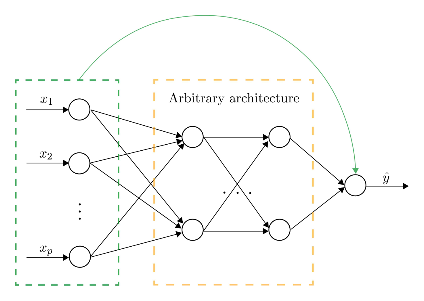
The architecture of LassoNet consists of a single residual connection, shown in green and an arbitrary feed-forward neural network, shown in black. The residual layer and the first hidden layer jointly pass through a hierarchical soft-thresholding optimizer.
3.2 Formulation
The LassoNet objective function is defined as
| (2) |
where the loss function was defined above in Section 3.1, and denotes the weights for feature in the first hidden layer. We emphasize that our goal is not just to sparsify the network, but to do so in a structured way that selects the relevant input features for the entire network. Since the network is feed-forward, we do not need to penalize the weights in remaining hidden layers.
The key idea in our approach is the constraint
This budgets the total amount of non-linearity involving feature according to the relative effect importance of as a main effect. An immediate consequence is that if . In other words, feature does not participate in the overall network if the skip-layer weight is zero. Hence control of the sparsity of the skip layer weights gives complete control of the feature sparsity in the network.
In the extreme case where , all the hidden units are inactive and only the skip connection remains. That is, the formulation recovers exactly the Lasso. In the other extreme (by letting ), one recovers a standard unregularized feed-forward neural network.
This formulation has several benefits. First, it promotes the linear component of the signal above the nonlinear one and uses it to guide feature sparsity. Such a strategy is not new, and bears close resemblance to the hierarchy principle which has been extensively studied in statistics (Choi et al. 2010; Radchenko and James 2010; Lim and Hastie 2014; She et al. 2016; Yan and Bien 2017). In addition, the formulation leverages the expressive power of residual neural networks (He et al. 2016). Finally, by tying every feature to a single coefficient (the linear component), our formulation provides a natural framework for feature selection.
One added benefit of the formulation is that the linear and non-linear components are fitted simultaneously, allowing the network to capture arbitrary nonlinearity in the data. If the best fitting model would have large but only moderate, this can be accommodated with a reasonable choice of . Furthermore, Fig. 4 suggests that the demand for hierarchy is analogous to the demand for sparsity—–a form of “regularization.”
Training LassoNet involves two operations. First, a vanilla gradient descent step is applied to all model parameters. Then, a hierarchical proximal operator is applied to the input layer pair . This sequential operation makes the procedure extremely simple to implement in popular machine learning frameworks, and requires only modifying a few lines of code from a standard residual network. The procedure is summarized in Alg. 1.
An added benefit of the method is its computational efficiency. The LassoNet regularization path can be trained at a cost that is essentially that of training a single model. This is achieved with the use of warm starts in a specific direction, as outlined in Section 4.1.
3.3 Hyper-parameter tuning
LassoNet has two hyper-parameters:
- •
the -penalty coefficient, , controls the complexity of the fitted model; higher values of encourage sparser models;
- •
the hierarchy coefficient, , controls the relative strength of the linear and nonlinear components.
It may be difficult to set the hierarchy coefficient without expert knowledge on the domain or task. We can circumvent this problem by treating the hierarchy coefficient as a hyper-parameter. We may use a naive search, which exhaustively evaluates the accuracy for the predefined hyper-parameter candidates with a validation dataset. This procedure can be performed in parallel.
4 Optimization
4.1 Warm starts: a path from dense to sparse
The technique of warm starts is very effective in optimizing models over an entire regularization path. For example, this technique is employed in Lasso -regularized linear regression (Friedman et al. 2010). In this approach, optimization is carried out for each fixed value of on a logarithmic scale from sparse to dense, and using the solution from the previous as a warm start for the next. This is effective, since the sparse models are easier to optimize and the sparse solution is often of main interest.
Somewhat surprisingly, to optimize LassoNet we find that a dense-to-sparse warm start approach is far more effective than a sparse-to-dense approach, in the sense that the former approach returns models that generalize better than those returned from the latter. This phenomenon is illustrated in Fig. 4, where the standard sparse-to-dense approach gets caught in local minima with poor generalization ability. On the other hand, the dense-to-sparse approach leverages the favorable generalization properties of the dense solution and preserves them after drifting into sparse local minima.


4.2 Hierarchical proximal optimization
The objective is optimized using proximal gradient descent, as outlined in Alg. 1. The key novelty is a numerically efficient algorithm for the proximal inner loop. We call the proposed algorithm Hier-Prox and detail it in Alg. 2. Underlying its development is the derivation of equivalent optimality conditions that completely characterize the global solution of the non-convex minimization problem defining the proximal operator. As it turns out, the inner loop is decomposable across features. As we show in Appendix B, Hier-Prox finds the global minimum of an optimization problem of the form
Remarkably, the complexity of Hier-Prox is controlled by , where is the total number of parameters being updated (i.e. ) This overhead is negligible compared to the computation of the gradients with respect to the same parameters. Furthermore, implementing the optimizer is straightforward in most standard deep learning frameworks. We provide more information about our implementation in Appendix D.
4.3 Computational Complexity
In most existing hierarchical models, computation remains a major challenge. Indeed, the complex nature of the regularizers used to enforce hierarchy prevents most current optimization algorithms from scaling with . In contrast, training LassoNet is performed at an attractive computational cost. Namely:
- •
The bulk of the computational cost occurs when training the dense network;
- •
Subsequently, training over the path is computationally cheap. By leveraging warm starts and the efficient Hier-Prox solver, the method effectively prunes the dense model. In practice, predictions across consecutive solutions in the path are usually close, which explains the speed-ups we observe in our experiments.
The use of warm starts dramatically reduces the number of rounds of gradient descent needed during each iteration, as the solution with penalty is often very similar to the solution with penalty . This added benefit distinguishes LassoNet from many competing feature selection methods, which require advance knowledge of the optimal number of features to select, and do not exhibit any computational savings over the path of features. Finally, the computational complexity of the method improves with hardware acceleration and parallelization techniques commonplace in deep learning.
4.4 Bias due to regularization
The use of the penalty slightly biases the weights of the model downwards. This is not exclusive to LassoNet, but is a well-known property of all regularized models such as Lasso (Lee et al. 2016). If the goal is to perform feature selection, this has no consequence on the training of LassoNet. If the goal is to get optimal predictive performance, it can be helpful to de-bias LassoNet. Our approach to do so is by re-training the network from scratch, restricting the input features to the subset of interest and zeroing out all others. In practice, this re-fitting tends to improve test-time performance. In addition, its computational overhead is relatively minor: (1) it is only needed after model selection, and therefore need not be performed on the entire regularization path; (2) the training time of the reduced model is relatively light if one uses the previous (biased) model as initialization in the gradient descent.
5 Experiments
In this section, we show experimental results on real-world datasets.
5.1 Data Sets
These datasets are drawn from several domains including protein data, image data and voice data, and have all been used for benchmarking feature selection methods in prior literature (Abid et al. 2019)33 3 The dataset descriptions were provided by these authors. (the size of the datasets can be found in Table 1):
- •
Mice Protein Dataset consists of protein expression levels measured in the cortex of normal and trisomic mice who had been exposed to different experimental conditions. Each feature is the expression level of one protein. 44 4 This data set has a few missing values, which we impute by column-means.
- •
MNIST and MNIST-Fashion consist of 28-by-28 grayscale images of hand-written digits and clothing items, respectively. We choose these datasets because they are widely known in the machine learning community. Although these are image datasets, the objects in each image are centered, which means we can meaningfully treat each 784 pixels in the image as a separate feature.
- •
ISOLET consists of preprocessed speech data of people speaking the names of the letters in the English alphabet, and is widely used as a benchmark in the feature selection literature. Each feature is one of the 617 quantities produced as a result of preprocessing, including spectral coefficients and sonorant features.
- •
COIL-20 consists of centered grayscale images of 20 objects. Images of the objects were taken at pose intervals of 5 degrees amounting to 72 images for each object. During preprocessing, the images were resized to produce 20-by-20 images, with each feature being one of the 400 pixels.
- •
Smartphone Dataset for Human Activity Recognition consists of sensor data collected from a smartphone mounted on subjects while they performed several activities such as walking upstairs, standing and laying. Each feature represents one of the 561 raw or processed quantities from the sensors on the phone.
5.2 Methodology
We compare LassoNet with several supervised feature selection methods mentioned in the Related Works Section, including HSIC-LASSO and the Fisher Score.
We also include principal feature analysis (PFA), a popular method for selecting discrete features based on PCA, proposed by Lu et al. 2007.
Where available, we made use of the scikit-feature implementation (Li et al. 2018) of each method.
Fig. 5 shows the results on the ISOLET data set , which is widely used as a benchmark in prior feature selection literature (Xue et al. 2020; Doquet and Sebag 2019).
We benchmarked each feature selection method with varying number of features. Although LassoNet is an integrated procedure — simultaneously performing feature selection and learning, most other methods are not, and therefore we explore the use of the selected feature set as input into two separate downstream learners.
In our experiments, we also include, as an upper-bound on performance, reconstruction methods that are not restricted to choosing individual features. In experiments with decoders, we use a standard feed-forward auto-encoder with all the input features, and in tree-based learners, we use equivalent full trees.
For every task, we run each algorithm being evaluated to extract the features selected. We measure classification accuracy by passing the resulting matrix to a one-hidden-layer feed-forward network and to an extremely randomized trees classifier (Geurts et al. 2006), a variant of random forests that has been used with feature selection methods in prior literature (Drotár et al. 2015). We chose these two classifiers to emphasize the inherent value of the selected features: since decoders and random forests are very different classifiers by nature, Figure 5 (for the ISOLET data set) indicates that the selected features are intrinsically informative (regardless of the classifier).
For all of the experiments, we use Adam optimizer with a learning rate of to train the initial dense model. Then, we use vanilla gradient descent with momentum equal to on the regularization path. See Appendix D for the architecture of the networks. For LassoNet, we did not use the network that was learned during training, but re-trained the feed-forward network from scratch. We divide each data set randomly into train, validation and test with a 70-10-20 split. The number of neurons in the hidden layer of the feed-forward network was varied within , and the network with the highest validation accuracy was selected and measured on the test set.
5.3 Results
The resulting classification errors are shown in Table 1 for the decoder network, and in Appendix C for the tree-based classifier. Overall, we find that our method is the strongest performer in the large majority of cases. While occasionally more than one method achieves the best accuracy, we find that our method either ties or outperforms the remaining methods in all instances, suggesting that our hierarchical objective may be widely applicable for different learning tasks.
In addition to Table 1, Figure 5 shows the classification accuracies for varying number of features on the ISOLET data set. We also report the corresponding figures for the other data sets in Appendix A, with similar results and conclusions.
| Dataset | # Classes | All-Features | Fisher | HSIC-Lasso | PFA | LassoNet | |
|---|---|---|---|---|---|---|---|
| Mice Protein | (1080, 77) | 8 | 0.990 | 0.944 | 0.958 | 0.939 | 0.958 |
| MNIST | (10000, 784) | 10 | 0.928 | 0.813 | 0.870 | 0.873 | 0.873 |
| MNIST-Fashion | (10000, 784) | 10 | 0.833 | 0.671 | 0.785 | 0.793 | 0.800 |
| ISOLET | (7797, 617) | 26 | 0.953 | 0.793 | 0.877 | 0.863 | 0.885 |
| COIL-20 | (1440, 400) | 20 | 0.996 | 0.986 | 0.972 | 0.975 | 0.991 |
| Activity | (5744, 561) | 6 | 0.853 | 0.769 | 0.829 | 0.779 | 0.849 |
6 Extension to Unsupervised Feature Selection
6.1 Background


Left: 3 test images from each class of digits are shown, sampled at random.
Right: the reconstructed versions of the test images using LassoNet with an intermediate penalty level (corresponding to about 50 active features) show that generally the digit is identified correctly and some stylistic features, such as the orientation in the digit ”5” and the thickness in the digit ”7”, are preserved. (see Figures 7,8,9 which show the results of applying LassoNet to individual classes of digits.)
In certain applications, specific prediction tasks may not be known ahead of time, and thus it is important to develop methods that can identify a subset of features while allowing imputation of the remaining features with minimal distortion for arbitrary downstream tasks. Thus, an unsupervised approach becomes relevant in order to identify the most important features in the dataset, and whether there are redundant features that do not need to be measured.
In this section, we show how to adapt LassoNet to the unsupervised setting. As another potential use case, we note that the algorithm is appropriate for multi-response classification and regression as well. By selecting a common set of features, the method is able to borrow strength across outputs to impute several different but potentially related responses.
6.2 Training
LassoNet adapts to the unsupervised setting easily by replacing the neural network classifier with a decoder network. More precisely, we consider the reconstruction loss , where denotes the Frobenius matrix norm.
The pseudocode, shown below, is quite similar to that for training the standard LassoNet. The major difference is the use of the group-LASSO penalty rather than LASSO in order to enforce the same set of selected features across all reconstructed inputs, leading to the Group-Hier-Prox algorithm.
6.3 Selected Digits for Single Classes in MNIST
We trained LassoNet in this unsupervised manner on subsets of the MNIST data consisting of a single digit. Some representative images for different digit classes are shown in Figs. 7, 8 and 9.


7 Extension to Matrix Completion
In several problems of contemporary interest, arising for instance in biomedical settings where measurements are costly or otherwise limited, the observed data are in the form of a large sparse matrix, , where . Popularly dubbed the matrix completion problem (Candès and Recht 2008; Mazumder et al. 2010), the task is to predict the unobserved entries.
Many existing approaches to the problem (Rennie and Srebro 2005; Bennett et al. 2007; Srebro 2004), including the popular Soft-Impute algorithm (Mazumder et al. 2010) make low-rank assumptions about the underlying matrix. In this section, we propose an extension of LassoNet that provides a new matrix completion method that does not make any low-rank assumption. Our method is detailed in Algorithm 5, and differs from Soft-Impute in two major aspects:
- •
First, it trains a feed-forward neural network on the imputation task. Our method is also iterative and updates the input using the reconstruction from the feed-forward network. Here the reconstruction loss is , where denotes the Frobenius norm. In Soft-Impute, the corresponding operation is singular value thresholding (that is, singular value decomposition followed by soft-thresholding) and finds a linear low-dimensional structure. In contrast, our method uses a nonlinear low-dimensional manifold through the network’s hidden layers.
- •
Once the dense model has been trained, the method performs feature selection using the Group-Hier-Prox operator (presented in Algorithm 4). This allows to prune the original imputation model so that it only uses a small set of input features.
To investigate the method’s performance, we run both LassoNet and Soft-Impute on the MICE Protein Dataset. This dataset was previously used in Section 5 for the supervised prediction task. Here the goal is to impute the entries that are missing from the training data. Initially, the data is complete with no missing entries (up to the few missing values we mentioned in Section 5.1. We construct our training set by keeping of the entries at random. We use of the data for validating hyper-parameters and for determining the stopping criterion. Finally, we reserve of the data for the hold-out test test. To control for the performance of the reconstruction network, we trained each reconstruction network using early stopping with a patience of epochs. Similarly to Section 5, we did not use the network that was learned during training, but retrained the reconstruction network from scratch. The results are displayed in Figure 10, where LassoNet achieves about a 50% reduction in the number of proteins measured for an equivalent test MSE. More details on the experimental settings are provided in Appendix D.


Our results show that the low-rank assumption underlying most existing matrix imputation methods is not always the most appropriate. More worryingly, when the linear assumption is violated, the statistical performance of standard imputation methods may be severely impaired. Therefore, it may be more reasonable to expect an arbitrary nonlinear low-dimensional structure. If that is the case, LassoNet will outperform linear reconstruction.
Finally, our method provides the added benefit of feature selection, which is of independent interest when measuring different features is costly or otherwise unavailable.
8 Sparsity in Learned Features
In some problems, the raw features are not interpretable and hence inducing sparsity in these features is not helpful:
- •
For example in computer vision, the inputs are pixels and without perfect registration, a given pixel does not even have the same meaning across different images. In this case, one may instead want to select visual shapes or patterns. The current practice of convolutional neural networks shies away from hand-engineered features and learns these from the data instead (Neyshabur 2020). Currently, the state-of-the-art is based on learning these convolutional filters. In this setting, it would be desirable to achieve “filter sparsity”, that is, select the most relevant convolutional filters. This can improve the interpretability of the model and alleviate the need for architecture search. In future work, we plan to achieve this by applying LassoNet to the output of one or more convolutional layers.
- •
Another application area is that of auto-encoders, whose bottleneck layer learns the most representative latent variables. Again, it is often of interest to further reduce the complexity of the auto-encoder by selecting the most important hidden units. We believe this is another promising direction for future research.
9 Discussion
In this paper, we have proposed a new feature selection method for neural networks. Unlike most other feature selection methods, our method is data-driven and provides a path of regularized models at a cost that is essentially that of training a single model. At its core, LassoNet involves a nonconvex optimization problem with hierarchy constraints to satisfy feature sparsity. By using proximal gradient descent, the nonconvex optimization problem is decomposed into two subproblems that are solved iteratively, one using stochastic gradient descent and the other analytically. The stochasticity of the initial dense model allows it to efficiently explore and converge over an entire regularization path with varying number of input features. This makes LassoNet different from many feature selection methods, which assume prior knowledge of the number of features to select.
Advantages of LassoNet include its generality and ease of use. First, the generality of the method allows it to extend to several other learning tasks, such as unsupervised reconstruction and matrix completion. Second, implementing the architecture in popular machine learning frameworks requires only modifying a few lines of code from a standard feed-forward neural network. Furthermore, the runtime of LassoNet over an entire path of feature sizes is similar to that of training a single model and improves with hardware acceleration and parallelization techniques commonplace in deep learning. Finally, the only additional hyperparameter of LassoNet is the hierarchy coefficient. We find that the default value, , used in this paper works well for a variety of datasets.
LassoNet, like the other feature selection methods we compared with in this paper, does not provide -values or statistical significance quantification. Features discovered through LassoNet should be validated through hypothesis testing or additional analysis using relevant domain knowledge. In this regard, a growing body of research about hypothesis testing for Lasso (Lockhart et al. 2014; Javanmard and Montanari 2014; Taylor and Tibshirani 2015) could serve as a fruitful starting point.
Python code and documentation for LassoNet is available at https://lassonet.ml, and R code will soon be available in the same website.
acknowledgments-disclosure-of-funding.
We would like to thank John Duchi and Ryan Tibshirani for helpful comments. Robert Tibshirani was supported by NIH grant 5R01 EB001988-16 and NSF grant 19 DMS1208164.References
- Abid et al. (2019) A. Abid, M. F. Balin, and J. Zou. Concrete autoencoders for differentiable feature selection and reconstruction. arXiv preprint arXiv:1901.09346, 2019.
- Amaldi et al. (1998) E. Amaldi, V. Kann, et al. On the approximability of minimizing nonzero variables or unsatisfied relations in linear systems. Theoretical Computer Science, 209(1-2), 1998.
- Bennett et al. (2007) J. Bennett, C. Elkan, B. Liu, P. Smyth, and D. Tikk. Kdd cup and workshop 2007. ACM SIGKDD Explorations Newsletter, 9(2):51–52, 2007.
- Cai et al. (2018) J. Cai, J. Luo, S. Wang, and S. Yang. Feature selection in machine learning: A new perspective. Neurocomputing, 300:70–79, 2018.
- Candès and Recht (2008) E. Candès and B. Recht. Exact matrix completion via convex optimization. Foundations of Computational Mathematics, 2008. doi: 10.1007/s10208-009-9045-5. URL http://dx.doi.org/10.1007/s10208-009-9045-5.
- Chandrashekar and Sahin (2014) G. Chandrashekar and F. Sahin. A survey on feature selection methods. Computers & Electrical Engineering, 40(1):16–28, 2014.
- Chen et al. (2017) J. Chen, M. Stern, M. J. Wainwright, and M. I. Jordan. Kernel feature selection via conditional covariance minimization. In Advances in Neural Information Processing Systems, pages 6946–6955, 2017.
- Choi et al. (2010) N. H. Choi, W. Li, and J. Zhu. Variable selection with the strong heredity constraint and its oracle property. Journal of the American Statistical Association, 105(489):354–364, 2010.
- Doquet and Sebag (2019) G. Doquet and M. Sebag. Agnostic feature selection. In Joint European Conference on Machine Learning and Knowledge Discovery in Databases, pages 343–358. Springer, 2019.
- Drotár et al. (2015) P. Drotár, J. Gazda, and Z. Smékal. An experimental comparison of feature selection methods on two-class biomedical datasets. Computers in biology and medicine, 66:1–10, 2015.
- Dua and Graff (2017) D. Dua and C. Graff. UCI machine learning repository, 2017. URL http://archive.ics.uci.edu/ml.
- Feng and Simon (2017) J. Feng and N. Simon. Sparse-input neural networks for high-dimensional nonparametric regression and classification. arXiv preprint arXiv:1711.07592, 2017.
- Friedman et al. (2010) J. Friedman, T. Hastie, and R. Tibshirani. Regularization paths for generalized linear models via coordinate descent. Journal of Statistical Software, 33:1–22, 2010.
- Geurts et al. (2006) P. Geurts, D. Ernst, and L. Wehenkel. Extremely randomized trees. Machine learning, 63(1):3–42, 2006.
- Gu et al. (2012) Q. Gu, Z. Li, and J. Han. Generalized fisher score for feature selection. arXiv preprint arXiv:1202.3725, 2012.
- Guyon and Elisseeff (2003) I. Guyon and A. Elisseeff. An introduction to variable and feature selection. Journal of Machine Learning Research, 55:1157–1182, 03 2003. doi: 10.1023/A:1024068626366.
- He et al. (2016) K. He, X. Zhang, S. Ren, and J. Sun. Deep residual learning for image recognition. In Proceedings of the IEEE conference on computer vision and pattern recognition, pages 770–778, 2016.
- Higuera et al. (2015) C. Higuera, K. J. Gardiner, and K. J. Cios. Self-organizing feature maps identify proteins critical to learning in a mouse model of down syndrome. PloS one, 10(6):e0129126, 2015.
- Javanmard and Montanari (2014) A. Javanmard and A. Montanari. Confidence intervals and hypothesis testing for high-dimensional regression. The Journal of Machine Learning Research, 15(1):2869–2909, 2014.
- Lee et al. (2016) J. D. Lee, D. L. Sun, Y. Sun, J. E. Taylor, et al. Exact post-selection inference, with application to the lasso. Annals of Statistics, 44(3):907–927, 2016.
- Li et al. (2017) J. Li, K. Cheng, S. Wang, F. Morstatter, R. P. Trevino, J. Tang, and H. Liu. Feature selection: A data perspective. ACM Computing Surveys (CSUR), 50(6):1–45, 2017.
- Li et al. (2018) J. Li, K. Cheng, S. Wang, F. Morstatter, R. P. Trevino, J. Tang, and H. Liu. Feature selection: A data perspective. ACM Computing Surveys (CSUR), 50(6):94, 2018.
- Lim and Hastie (2014) M. Lim and T. Hastie. Learning interactions via hierarchical group-lasso regularization. Journal of Computational and Graphical Statistics, pages 1–41, 2014.
- Lin and Jegelka (2018) H. Lin and S. Jegelka. Resnet with one-neuron hidden layers is a universal approximator. In Advances in neural information processing systems, pages 6169–6178, 2018.
- Lockhart et al. (2014) R. Lockhart, J. Taylor, R. J. Tibshirani, and R. Tibshirani. A significance test for the lasso. Annals of statistics, 42(2):413, 2014.
- Lu et al. (2007) Y. Lu, I. Cohen, X. S. Zhou, and Q. Tian. Feature selection using principal feature analysis. In Proceedings of the 15th ACM international conference on Multimedia, pages 301–304, 2007.
- Mazumder et al. (2010) R. Mazumder, T. Hastie, and R. Tibshirani. Spectral regularization algorithms for learning large incomplete matrices. J. Mach. Learn. Res., 11:2287¿2322, 2010.
- Min et al. (2014) F. Min, Q. Hu, and W. Zhu. Feature selection with test cost constraint. International Journal of Approximate Reasoning, 55(1):167–179, 2014.
- Neyshabur (2020) B. Neyshabur. Towards learning convolutions from scratch. arXiv preprint arXiv:2007.13657, 2020.
- Radchenko and James (2010) P. Radchenko and G. M. James. Variable selection using adaptive nonlinear interaction structures in high dimensions. Journal of the American Statistical Association, 105(492):1541–1553, 2010.
- Raghu et al. (2017) M. Raghu, B. Poole, J. Kleinberg, S. Ganguli, and J. Sohl-Dickstein. On the expressive power of deep neural networks. In international conference on machine learning, pages 2847–2854, 2017.
- Rennie and Srebro (2005) J. D. Rennie and N. Srebro. Fast maximum margin matrix factorization for collaborative prediction. In Proceedings of the 22nd international conference on Machine learning, pages 713–719, 2005.
- Ribeiro et al. (2016) M. T. Ribeiro, S. Singh, and C. Guestrin. ” why should i trust you?” explaining the predictions of any classifier. In Proceedings of the 22nd ACM SIGKDD international conference on knowledge discovery and data mining, pages 1135–1144, 2016.
- She et al. (2016) Y. She, Z. Wang, and H. Jiang. Group regularized estimation under structural hierarchy. Journal of the American Statistical Association, 0(ja):0–0, 2016. doi: 10.1080/01621459.2016.1260470. URL https://doi.org/10.1080/01621459.2016.1260470.
- Song et al. (2012) L. Song, A. Smola, A. Gretton, J. Bedo, and K. Borgwardt. Feature selection via dependence maximization. Journal of Machine Learning Research, 13(5), 2012.
- Srebro (2004) N. Srebro. Learning with matrix factorizations. Ph.D Thesis, 2004.
- Taylor and Tibshirani (2015) J. Taylor and R. J. Tibshirani. Statistical learning and selective inference. Proceedings of the National Academy of Sciences, 112(25):7629–7634, 2015.
- Tibshirani (1996) R. Tibshirani. Regression shrinkage and selection via the lasso. Journal of the Royal Statistical Society, Series B, 58:267–288, 1996.
- Wulfkuhle et al. (2003) J. D. Wulfkuhle, L. A. Liotta, and E. F. Petricoin. Proteomic applications for the early detection of cancer. Nature reviews cancer, 3(4):267–275, 2003.
- Xue et al. (2020) H. Xue, Y. Song, and H.-M. Xu. Multiple indefinite kernel learning for feature selection. Knowledge-Based Systems, 191:105272, 2020.
- Yamada et al. (2014) M. Yamada, W. Jitkrittum, L. Sigal, E. P. Xing, and M. Sugiyama. High-dimensional feature selection by feature-wise kernelized lasso. Neural computation, 26(1):185–207, 2014.
- Yan and Bien (2017) X. Yan and J. Bien. Hierarchical sparse modeling: A choice of two group lasso formulations. Statist. Sci., 32(4):531–560, 11 2017. doi: 10.1214/17-STS622. URL https://doi.org/10.1214/17-STS622.
Appendix A Additional Experiments
In this section, we report the results for different numbers of features on the other data sets, similar to what was done for the ISOLET data set in Figure 5. These figures complement Table 1 where the number of features was fixed to . Overall, we find that LassoNet continues to achieve high (though not always highest) accuracy.
We note that for all methods other than LassoNet, the computational cost of producing these figures was multiples of that of producing the table. This is because most other feature selection methods take as input , the number of features to select, and need to run from scratch for diferent values of . On the other hand, for LassoNet the cost remains essentially unchanged. We refer the reader to Section 4.3 for further discussion.
Appendix B Proofs
Proof of Correctness of the Hier-Prox and Group-Hier-Prox Operators
At its core, LassoNet performs a step of vanilla gradient descent and subsequently solves a constrained minimization problem. Since the problem is decomposable across features, each iteration of the algorithm decouples into single-feature optimization problems. Here we show the following:
- 1.
Hier-Prox returns the global optimum of the following optimization problem:
(3) where is a scalar and is a vector.
- 2.
Hier-Prox-Group returns the global optimum of the following problem:
(4) where , are vectors of the same size.
It turns out that the aforementioned two results are special cases of the following proposition. They can be easily recovered by setting .
Proposition 1.
Fix and . (Note: the two integers can be different) Let us consider the problem
We derive the sufficient and necessary condition for characterizing the global optimum of the above optimization problem:
- 1.
Let us order the coordinates in decreasing order
and define for each the value by
Then where is the unique such that
By convention and .
- 2.
The must satisfy
Proof.
We start by proving the claim below: for some
| (5) |
Denote . By definition, is the minimum of the below optimization problem:
Now that strong duality holds since Slater’s condition holds. Thereby, we know for some dual variable , minimizes the Lagrangian function below:
Now, let’s take subgradient and get that needs to satisfy,
| (6) |
Now we divide our discussion into two cases:
- 1.
. The KKT condition (Eq. (6)) shows for some . This implies that , which is possible if and only if .
- 2.
. The KKT condition (Eq. (6)) gives . Since for , it implies . Hence . Note if , then we must have . Thus, having some with is equivalent to that .
Summarizing the above discussion, we see that must satisfy
This proves the claim at Eq (5). Introduce the mapping
The claim at Eq (5) shows that it suffices to find that minimizes
Denote . Order the coordinates in decreasing order
Define by convention that and . Now, we compute the value when . Indeed, we have
where denotes the remainder term, which is independent of but can be dependent of , , , , , . Now, let’s define for
and denote to be the global minimum of on , i.e.,
Now we show the two claims below, which implies the desired proposition.
- (a)
There exists one unique such that
(7) - (b)
The global minimum .
Proof of Point
Denote to be the one that satisfies
It suffices to prove the existence and uniqueness of satisfying Eq (7). Introduce the function by
It is clear that is increasing w.r.t. . Moreover, by algebraic manipulation, one can show that satisfies
if and only if (set by convention , )
This proves the existence and uniqueness of that satisfies Eq (7).
Proof of Point
Introduce the function
We will show that
- (i)
is strictly increasing when and .
- (ii)
is strictly decreasing when and .
The above two facts imply that the global minimum of must belong to the interval . Thus is the global minimum of since achieves the minimum over all that satisfy .
Now we prove point and point . For , we know that . From all satisfying , it is clear that minimizes . Therefore, for ,
where denotes the remainder term, which is independent of but can be dependent of , , , , , . Now, by definition of , we know that
- (1)
for .
- (2)
for .
Simple algebraic manipulation shows that, this implies that
- (1)
for .
- (2)
for .
Note that is quadratic centered at for . This proves the desired deferred point and point . ∎
Appendix C Classification accuracies using tree-based classifiers as the downstream learner
Here we report the equivalent table to Table 1, but using the extremely randomized tree classifier as downstream learner. The results are competitive, as LassoNet continues to have high (but not always highest) classification accuracy.
| Dataset | # Classes | All-Feature | Fisher | HSIC-Lasso | PFA | LassoNet | |
|---|---|---|---|---|---|---|---|
| Mice Protein | (1080, 77) | 8 | 0.997 | 0.996 | 0.996 | 0.997 | 0.997 |
| MNIST | (10000, 784) | 10 | 0.941 | 0.818 | 0.869 | 0.879 | 0.892 |
| MNIST-Fashion | (10000, 784) | 10 | 0.831 | 0.66 | 0.775 | 0.784 | 0.794 |
| ISOLET | (7797, 617) | 26 | 0.951 | 0.818 | 0.888 | 0.855 | 0.891 |
| COIL-20 | (1440, 400) | 20 | 0.996 | 0.996 | 0.993 | 0.993 | 0.993 |
| Activity | (5744, 561) | 6 | 0.859 | 0.794 | 0.845 | 0.808 | 0.860 |
Appendix D Experimental Details
All experiments were run on a single computer with NVIDIA Tesla K80 and Intel Xeon E5-2640.
D.1 LassoNet Architecture
The implementation was conducted in the PyTorch framework. For LassoNet, we use a one-hidden-layer feed-forward neural network with ReLU activation function. We also included a two-hidden-layer network in Section 7 for the matrix completion problem. The number of neurons in the hidden layer was varied within , where is the total number of features, and the network with the highest validation accuracy was selected and measured on the test set. We used a learning rate of and early stopping criterion of . Although the hierarchy parameter could in principle be selected on a validation set as well, we have found that the default value works well for a variety of datasets.
D.2 Benchmark Datasets
The MNIST and MNIST-Fashion datasets were retrieved using their official source. The remaining datasets were retrieved from the UCI Repository [Dua and Graff 2017].