跳到论文正文
W Papers独立论文阅读器 arXiv:1907.12125 论文正文 计算阅读时间 · 0%
引用这篇论文根据当前论文元数据生成,正式投稿前建议核对。


License: arXiv.org perpetual non-exclusive license
arXiv:1907.12125v5 [math.OC] 24 Nov 2021

The Prescription Approach to Decentralized Stochastic Control with Word-of-Mouth Communication

Aditya Dave    Student Member, IEEE,    Andreas A. Malikopoulos    Senior Member, IEEE Thanks: This research was supported in part by ARPAE’s NEXTCAR program under the award number DE-AR0000796 and by the Delaware Energy Institute (DEI). Thanks: The authors are with the Department of Mechanical Engineering, University of Delaware, Newark, DE 19716 USA (email: adidave@udel.edu; andreas@udel.edu).
Abstract

In this paper, we analyze a network of agents that communicates through word of mouth. In a word-of-mouth communication system, every agent communicates with her neighbors with delays in communication. This is a non-classical information structure where the topological and temporal restrictions in communication mean that information propagates slowly through the network. We present the prescription approach to derive structural results for problems with word-of-mouth communication. The structural results lead to optimal control strategies in time-invariant spaces. We also present a comparison of our results with the common information approach.

Index Terms: 
Decentralized control, information structures, stochastic control, team theory, partially observable Markov decision processes.

I Introduction

The interdependence of many engineering systems can enable the development of a novel framework to process large amounts of data and deliver real-time control actions that optimize associated benefits. As we move to increasingly complex systems [1], new decentralized control approaches are needed to optimize the impact on system behavior of the interaction between its entities. Centralized stochastic control [2] has been a ubiquitous approach to control complex systems [3], and is well understood. It refers to multi-stage optimization problems with external disturbances and noisy observations controlled by a single decision maker. A key assumption is that the decision maker perfectly recalls all past control actions and observations. The information available to an agent when making a decision is called the information structure of the system. If every agent has access to the same information and a perfect recall of the information, the information structure is called the classical information structure. While centralized systems have been extensively studied, their core assumption does not hold for many applications involving multiple agents, e.g., connected automated vehicles [4], a swarm of drones [5], and smart grids [6]. In such systems, all agents simultaneously make a decision based only on their memory and local information received through communication with other agents. Such agent-to-agent communication might be generally delayed or costly [7]. Thus, it is not possible to compute a centralized estimate of the complete state of the system from the observation history of a single agent. Such multi-stage optimization problems [8] are known as decentralized stochastic control problems.

In this paper, we study a decentralized system with a word-of-mouth information structure. In the absence of any entity facilitating transmission of information among agents (a shared memory), the communication among agents occurs through the word of mouth. In a word-of-mouth communication, we model the system as a network of agents connected by communication links. An agent can directly communicate with her neighbors in the network, with some associated delays. Thus, information from each agent propagates through the network by her neighbors who share it with their neighbors, and so on. This problem has a non-classical information structure because of the delays in communication. Such a model can describe many different decentralized systems with limited communication. As an example, consider a team of drones that conducts a rescue operation at an inaccessible location. At any time, all drones simultaneously must make the best possible decision under asymmetric information. Due to hardware limitations, a drone can only communicate within a limited range. The range of the entire team of drones, however, may need to extend far beyond the range of a single drone. In this situation, the drones need to communicate through word of mouth to make optimal decisions.

I-A Related Work

Decentralized stochastic control is fundamentally different from and significantly more challenging than centralized stochastic control. The most common approach in centralized stochastic control is dynamic programming (DP), which is not directly applicable to decentralized systems since no general separation results between estimation and control are known [9]. Thus, new approaches are needed to address these problems. There are three general approaches in the literature that use techniques from centralized stochastic control.

The person-by-person approach aims to transform the problem into a centralized stochastic control problem from the point of view of a single agent. This is done by arbitrarily fixing the control strategies for all agents except for one agent i{i}. The control strategy of agent ii is then optimized for this new problem, assuming the fixed strategies used by the other agents are known to agent ii. This allows for the use of techniques from centralized stochastic control, including DP. This process is then repeated for all agents until a stable equilibrium is attained. This control strategy is called a person-by-person optimal strategy. In general, the solution is not globally optimal [10]. However, the solution’s structural properties may guarantee a time-invariant optimal strategy. An early application of this idea was found in problems of real-time communication using encoders and decoders [11, 12, 13, 14, 15]. The person-by-person approach has also been used in decentralized hypothesis testing and quickest detection problems [16]. Some other applications have appeared in networked control systems [17] and team decision problems with partially nested information structures [10, 18]. In special cases, such as team decision problems with static information structures and convex cost, the person-by-person solution is globally optimal [19].

The designer’s approach considers the point of view of a designer with knowledge of the model and statistics of all random variables in the system. The designer’s task is to choose the optimal control strategy, or design, for the system. This is done by transforming the problem into a centralized planning problem, and then using DP to derive the optimal strategy. The control action for the designer’s planning problem is the control law that the designer assigns to each agent at each time step. DP ensures global optimality of these assignments. However, the designer’s approach, first introduced by Witsenhausen [20] for general models, suffers from high computational complexity. This approach was later applied in controls with a fixed memory [21]. This approach was further developed in [22].

The most recent approach in decentralized control is the common information approach, first presented for problems with partial history sharing [23], [24], where each agent shares a subset of her past observations and control actions to a shared memory accessible to every agent in the system. Then, each agent makes a decision using information available in the shared memory (the common information) and the recall of her own history. The solution is derived by reformulating the system from the viewpoint of a fictitious coordinator with access only to the shared information, whose task is to prescribe control strategies to each agent. This approach has been used to derive structural results and a DP decomposition for problems with delayed information to the shared memory [24]. Structural results are properties of optimal control strategies that address how we can compress information that is increasing with time to a sufficient statistic that takes values in a time-invariant space. The common information approach has also been used in problems with control sharing information structure [25], stochastic games with asymmetric information [26] and teams with mean-field sharing [27]. There are also some earlier papers that used similar ideas to analyze specific information structures [28, 29, 30].

I-B Contributions

The common information approach is considered as the standard approach to analyze systems with a word-of-mouth information structure. However, when the maximum delay in communication across agents is large, the common information approach can lead to a large number of computations to derive the optimal strategies. This has motivated us to develop the prescription approach for systems with different delays in communication among different agents. Some related preliminary results can be found in [31, 32].

The contributions of this paper are: We present the prescription approach that leads to improved structural results for decentralized systems with a word-of-mouth information structure. These structural results lead to a smaller search space for optimal strategies when compared to the common information approach (see Section V-B for details), or any other approach. The structural properties and derivations of our results are distinct from existing results in literature. In fact, the common information approach can be considered as a special case of the prescription approach. Furthermore, our results are applicable to a wide range of decentralized control problems with delayed, asymmetric information sharing among agents.

I-C A static system

In this subsection, we present a simple example to illustrate the main idea behind the prescription approach and make a comparison with the common information approach. Consider a static system with three agents. Let XX denote the state of the system and Y1,Y2,Y3Y^{1},\;Y^{2},\;Y^{3} be the observations of each agent about XX. All random variables are binary and their joint probability distribution is known. The information available to agents 11, 22, and 33 is M1={Y1,Y2,Y3}M^{1}=\{Y^{1},Y^{2},Y^{3}\}, M2={Y2,Y3}M^{2}=\{Y^{2},Y^{3}\}, and M3={Y3}M^{3}=\{Y^{3}\}, respectively. Every agent k∈{1,2,3}k\in\{1,2,3\} selects a control action as Uk=gk​(Mk)U^{k}=g^{k}(M^{k}) and the system incurs a cost c⁡(X,U1,U2,U3)c(X,U^{1},U^{2},U^{3}). The problem is to find the control strategy 𝒈=(g1,g2,g3)\bm{g}=(g^{1},g^{2},g^{3}) that minimizes the performance criterion 𝒥⁡(𝒈)=𝔼𝒈​[c⁡(X,U1,U2,U3)]\mathcal{J}(\bm{g})=\mathbb{E}^{\bm{g}}[c(X,U^{1},U^{2},U^{3})]. Using a brute force search, we would have to compute the performance of 28×24×22=16,3842^{8}\times 2^{4}\times 2^{2}=16,384 strategies before arriving at the optimal control strategy.

The key idea of this paper is to partition the memory of different agents into accessible and inaccessible information to simplify the search for optimal strategies. We formally define these terms in Section III-A. Here, we simply note that the accessible information of agents 11, 22, and 33 are A1={Y1,Y2,Y3}A^{1}=\{Y^{1},Y^{2},Y^{3}\}, A2={Y2,Y3}A^{2}=\{Y^{2},Y^{3}\}, and A3={Y3}A^{3}=\{Y^{3}\}, respectively. The accessible information of agent 33 is also the common information in the system. The inaccessible information of agent 11 with respect to agent 11 is L[1,1]=∅L^{[{{1}},{{1}}]}=\emptyset, with respect to agent 22 is L[1,2]={Y1}L^{[{{1}},{{2}}]}=\{Y^{1}\}, and with respect to agent 33 is L[1,3]={Y1,Y2}L^{[{{1}},{{3}}]}=\{Y^{1},Y^{2}\}. Similarly, the inaccessible information of agent 22 with respect to agent 22 is L[2,2]=∅L^{[{{2}},{{2}}]}=\emptyset, and with respect to agent 33 is L[2,3]={Y2}L^{[{{2}},{{3}}]}=\{Y^{2}\}. Finally, the inaccessible information of agent 33 with respect to agent 33 is L[3,3]=∅L^{[{{3}},{{3}}]}=\emptyset. Note that M1=A1∪L[1,1]=A2∪L[1,2]M^{1}=A^{1}\cup L^{[1,1]}=A^{2}\cup L^{[1,2]} and so on.

Now we consider that every agent k∈{1,2,3}k\in\{1,2,3\} generates prescriptions (Γ[k,1],Γ[k,2],Γ[k,3])(\Gamma^{[k,1]},\Gamma^{[k,2]},\Gamma^{[k,3]}) corresponding to every other agent in {1,2,3}\{1,2,3\}, respectively, by only observing the accessible information AkA^{k}. The prescription Γ[k,i]\Gamma^{[k,i]} is a mapping from the inaccessible information L[i,k]L^{[i,k]} to the control action UiU^{i}. Thus, for agent 33, for every k∈{1,2,3}k\in\{1,2,3\}, we can write Γ[3,k]=ψ[3,k]​(A3)=ψ[3,k]​(Y3),\Gamma^{[{{3}},{{k}}]}=\psi^{[{{3}},{{k}}]}(A^{3})=\psi^{[{{3}},{{k}}]}(Y^{3}), where ψ[3,k]\psi^{[{{3}},{{k}}]} is the prescription law for the prescription of agent 33 for agent kk. Let Γn[3,k]=ψ[3,k]​(Y3=n)\Gamma^{[{{3}},{{k}}]}_{n}=\psi^{[{{3}},{{k}}]}(Y^{3}=n) for n∈{0,1}n\in\{0,1\}. Then, the performance criterion for agent 33 is given by

𝒥⁡(𝝍3)=𝔼𝝍3​[c⁡(X,U1,U2,U3)]\displaystyle\mathcal{J}(\bm{\psi}^{3})=\mathbb{E}^{\bm{\psi}^{3}}[c(X,U^{1},U^{2},U^{3})]
=∑n∈{0,1}ℙ(Y3=n)⋅𝔼𝝍3[c(\displaystyle=\sum_{n\in\{0,1\}}\mathbb{P}(Y^{3}=n)\cdot\mathbb{E}^{\bm{\psi}^{3}}\Big[c\big( X,Γn[3,1]​(Y1,Y2),\displaystyle X,\Gamma^{[{{3}},{{1}}]}_{n}(Y^{{1}},Y^{{2}}),
Γn[3,2](Y2),Γn[3,3])|Y3=n],\displaystyle\Gamma^{[{{3}},{{2}}]}_{n}(Y^{{2}}),\Gamma^{[{{3}},{{3}}]}_{n}\big)|Y^{3}=n\Big],

where 𝝍3=(ψ[3,1],ψ[3,2],ψ[3,3])\bm{\psi}^{3}=(\psi^{[{{3}},{{1}}]},\psi^{[{{3}},{{2}}]},\psi^{[{{3}},{{3}}]}). Minimizing the performance criterion above is equivalent to minimizing the original expected cost (see Lemma 5). In this new cost, we can minimize the two terms separately, leading to a computation of (24×22×2)+(24×22×2)=256(2^{4}\times 2^{2}\times 2)+(2^{4}\times 2^{2}\times 2)=256 strategies. Note that the number prescriptions obtained for agent 33 are the same as those obtained using the common information approach in [23]. Thus, the common information approach also leads to a computation of 256256 strategies.

Now, consider the prescriptions for agent 22. For k∈{1,2}k\in\{1,2\}, we have Γ[2,k]=ψ[2,k]​(A2)=ψ[2,k]​(Y2,Y3)\Gamma^{[{{2}},{{k}}]}=\psi^{[{{2}},{{k}}]}(A^{2})=\psi^{[{{2}},{{k}}]}(Y^{2},Y^{3}), where ψ[2,k]\psi^{[{{2}},{{k}}]} is the prescription law for the prescription of agent 22 for agent kk. For the case k=3k=3, Γ[2,3]=Γ[3,3]\Gamma^{[{{2}},{{3}}]}=\Gamma^{[{{3}},{{3}}]} (see Lemmas 3-4). Let Γm,n[3,k]=ψ[3,k]​(Y2=m,Y3=n)\Gamma^{[{{3}},{{k}}]}_{m,n}=\psi^{[{{3}},{{k}}]}(Y^{2}=m,Y^{3}=n), n,m∈{0,1}n,m\in\{0,1\} and k∈{1,2}k\in\{1,2\}. The performance criterion for agent 22 is

𝒥⁡(𝝍2)=𝔼𝝍2​[c⁡(X,U1,U2,U3)]=∑m,n∈{0,1}ℙ⁡(Y2=m,Y3=n)⋅𝔼𝝍2[c(X,Γ[2,1]m,n(Y1),Γ[2,2]m,n,Γ[3,3]n)|Y2=m,Y3=n],\mathcal{J}(\bm{\psi}^{2})=\mathbb{E}^{\bm{\psi}^{2}}[c(X,U^{1},U^{2},U^{3})]\\ =\sum_{m,n\in\{0,1\}}\mathbb{P}(Y^{2}=m,Y^{3}=n)\\ \cdot\mathbb{E}^{\bm{\psi}^{2}}\Big[c\big(X,\Gamma^{[{{2}},{{1}}]}_{m,n}(Y^{{1}}),\Gamma^{[{{2}},{{2}}]}_{m,n},\Gamma^{[{{3}},{{3}}]}_{n}\big)|Y^{2}=m,Y^{3}=n\Big],

where 𝝍2=(ψ[2,1],ψ[2,2],ψ[2,3])\bm{\psi}^{2}=(\psi^{[{{2}},{{1}}]},\psi^{[{{2}},{{2}}]},\psi^{[{{2}},{{3}}]}). We show in Lemma 5 that the optimal cost achieved by agent 22 is the same as the one of agent 33. However, in the cost for agent 22, we can minimize the four terms separately, having to compute only (22×2×2)×4=64(2^{2}\times 2\times 2)\times 4=64 strategies. Using a similar procedure, we can show that the optimal prescription strategy for agent 11 can also be obtained with 6464 computations. Note that the cost for agents 11, 22, and 33 are different, but all lead to the same optimal cost. The costs for agents 11 and 22 lead to an improvement in computation time of optimal strategies when compared to the common information approach. This example shows that even in static systems, there are avenues beyond the common information approach to improve the computation time for optimal strategies.

Remark 1.

Consider a larger set of agents 𝒦={1,…,K}\mathcal{K}=\{1,\dots,K\}, with the same information structure Mk+1⊆MkM^{k+1}\subseteq M^{k}, k∈𝒦∖{K}k\in\mathcal{K}\setminus\{K\}. The agent KK must still compute the same number of strategies as in the common information approach. However, the number of computations decreases with the index of the agent from KK all the way to 11, implying that the fastest computation of optimal strategies is achieved by agent 11.

I-D Organization

The remainder of the paper is organized as follows: In Section II, we present the model of the decentralized stochastic problem with a word-of-mouth information structure. In section III, we introduce the prescription approach along with the associated properties of the prescription functions. In Section IV, we use the prescription approach to derive structural results from the point of view of various agents in the system. In Section V, we simplify the structural results and compare them with the common information approach. Finally, we conclude with some observations and future research directions in Section VI.

II Problem Formulation

II-A Network Description

Consider a directed network of K∈ℕK\in\mathbb{N} agents represented by a strongly connected graph 𝒢=(𝒦,ℰ)\mathcal{G}=(\mathcal{K},\mathcal{E}), where 𝒦:={1,…,K}\mathcal{K}:=\{1,\dots,K\} is the set of agents and ℰ\mathcal{E} is the set of links. A direct communication link from any agent k∈𝒦k\in\mathcal{K} to any agent j∈𝒦j\in\mathcal{K} is denoted by (k,j)∈ℰ(k,j)\in\mathcal{E}, which is characterized by a delay of δ[k,j]∈ℕ\delta^{[{{k}},{{j}}]}\in\mathbb{N} time steps for transferring information from kk to jj.

When agent kk sends out information to some agent jj in her neighborhood, we call the act transmission of information. The information transmitted by agent kk at time t∈ℕt\in\mathbb{N} is received by agent jj at time t+δ[k,j]t+\delta^{[{{k}},{{j}}]}. For any agent kk, the acts of reception and transmission of information occur at different instances within every time step, as discussed in Section II-D.

Definition 1.

For two agents k,j∈𝒦k,j\in\mathcal{K}, a path qa[k,j]q^{[{{k}},{{j}}]}_{a}, a∈ℕa\in\mathbb{N}, from kk to jj is the sequence {kn}n=1m\{k_{n}\}_{n=1}^{m}, m∈𝒦m\in\mathcal{K}, such that: (1) k1=kk_{1}=k and km=jk_{m}=j, (2) kn∈𝒦k_{n}\in\mathcal{K} for n∈𝒦n\in\mathcal{K}, and (3) there exists a link (kn−1,kn)∈ℰ(k_{n-1},k_{n})\in\mathcal{E} for n∈𝒦∖{1}n\in\mathcal{K}\setminus\{1\}.

Let 𝒬[k,j]={qa[k,j]:a∈ℕ}\mathcal{Q}^{[{{k}},{{j}}]}=\{q^{[{{k}},{{j}}]}_{a}:a\in\mathbb{N}\} be the set with all paths from agent kk to agent jj.

Definition 2.

Consider agents k,j∈𝒦k,j\in\mathcal{K} with a path qa[k,j]∈𝒬[k,j]q^{[{{k}},{{j}}]}_{a}\in\mathcal{Q}^{[{{k}},{{j}}]}. The communication delay da[k,j]∈ℕd^{[{{k}},{{j}}]}_{a}\in\mathbb{N} for qa[k,j]q^{[{{k}},{{j}}]}_{a} is da[k,j]=δ[k,k2]+⋯+δ[km−1,j],d^{[{{k}},{{j}}]}_{a}=\delta^{[k,k_{2}]}+\dots+\delta^{[k_{m-1},j]}, where δ[kn−1,kn]\delta^{[k_{n-1},k_{n}]} is the delay in information transfer through the link (kn−1,kn)∈ℰ(k_{n-1},k_{n})\in\mathcal{E}.

The information path from agent kk to agent jj in the network is the path with the least possible delay.

Definition 3.

The information path from kk to jj, denoted by (k→j)(k\rightarrow j), is the path q[k,j]∈𝒬[k,j]q^{[{{k}},{{j}}]}\in\mathcal{Q}^{[{{k}},{{j}}]} such that d[k,j]=min⁡{d1[k,j],…,db[k,j]},d^{[{{k}},{{j}}]}=\min\left\{d_{1}^{[{{k}},{{j}}]},\dots,d_{b}^{[{{k}},{{j}}]}\right\}, where b:=|𝒬[k,j]|b:=|\mathcal{Q}^{[{{k}},{{j}}]}|.

The property of strong connectivity in our network ensures that there is always an information path (k→j)(k\rightarrow j) from every agent k∈𝒦k\in\mathcal{K} to every agent j∈𝒦j\in\mathcal{K}. When there are multiple paths with the same least delay, any of these paths can be designated to be the information path. We denote the delay associated with the information path (k→j)(k\rightarrow j) by d[k,j]d^{[{{k}},{{j}}]} and, by convention, let d[k,k]=0d^{[k,k]}=0. Since the links in the network are directed, the delay d[k,j]d^{[{{k}},{{j}}]} in communication from kk to jj is not necessarily the same as the delay d[j,k]d^{[j,k]} from jj to kk.

II-B System Description

The network of agents is considered a discrete-time system that evolves up to a finite time horizon T∈ℕT\in\mathbb{N}. At any time t=0,1,…,Tt=0,1,\dots,T, the state of the system XtX_{t} takes values in a finite set 𝒳\mathcal{X} and the control variable UtkU_{t}^{k} generated by agent k∈𝒦k\in\mathcal{K} takes values in a finite set 𝒰k\mathcal{U}^{k}. Let Ut1:K{U}_{t}^{1:K} denote the vector (Ut1,…,UtK)(U_{t}^{1},\dots,U_{t}^{K}). Starting at the initial state X0X_{0}, the evolution of the system follows the state equation

Xt+1=ft(Xt,Ut1:K,Wt),X_{t+1}=f_{t}\left(X_{t},U_{t}^{1:K},W_{t}\right), (1)

where WtW_{t} is the external disturbance to the system represented as a random variable taking values in a finite set 𝒲\mathcal{W}. At time tt every agent kk makes an observation YtkY_{t}^{k},

Ytk=htk​(Xt,Vtk),Y_{t}^{k}=h_{t}^{k}(X_{t},V_{t}^{k}), (2)

taking values in a finite set 𝒴k\mathcal{Y}^{k} through a noisy sensor, where VtkV_{t}^{k} takes values in the finite set 𝒱k\mathcal{V}^{k} and represents the noise in measurement. Agent kk selects a control action UtkU_{t}^{k} from the set of feasible control actions 𝒰k\mathcal{U}^{k} as a function of her information structure. The information structure is different for each agent k∈𝒦k\in\mathcal{K} because of the means of communication and topology of the network. We discuss the information structure in detail in Section II-E. After each agent kk generates a control action UtkU_{t}^{k}, the system incurs a cost ct​(Xt,Ut1,…,UtK)∈ℝc_{t}(X_{t},U_{t}^{1},\dots,U_{t}^{K})\in\mathbb{R}.

II-C Assumptions

In our modeling framework above, we impose the following assumptions:

Assumption 1.

The network topology is strongly connected with self-loops, known a priori, and does not change with time.

With a known and invariable network topology, every agent can keep track of what information is accessible to other agents in the network.

Assumption 2.

The external disturbances {Wt:t=0,…,T}\{W_{t}:t=0,\dots,T\} and noises in measurement {Vtk:t=0,…,T;k=1,…,K}\{V_{t}^{k}:t=0,\dots,T;k=1,\dots,K\} are sequences of independent random variables that are also independent of each other and of the initial state X0X_{0}.

The external disturbances, noises in measurement, and initial state are referred to as the primitive random variables, and their probability distributions are known to all decision makers. This allows us to analyse the system as a controlled Markov chain.

Assumption 3.

The state functions (ft:t=0,…,T)(f_{t}:t=0,\dots,T), observation functions (htk:t=0,…,T;k=1,…,K)(h_{t}^{k}:t=0,\dots,T;k=1,\dots,K), the cost functions (ct:t=0,…,T),(c_{t}:t=0,\dots,T), and the set of all feasible control strategies GG are known to all agents.

These functions and the set of feasible control strategies (defined in Section II-E) form the basis of the decision making problem.

Assumption 4.

Each agent perfectly recalls all information that enters her memory.

Perfect recall of the data from the memory of every agent is an essential assumption for the structural results derived in this paper.
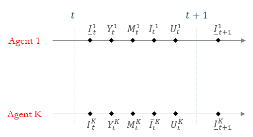
Refer to caption
Fig. 1: Sequence of activities

We summarize below the sequence of activities taken by agent k∈𝒦k\in\mathcal{K} at time tt (see Fig. 1):

  1. 1.

    The state XtX_{t} is updated based on (1).

  2. 2.

    Agent kk receives information from all agents in 𝒦\mathcal{K}, denoted by I¯tk\underline{I}_{t}^{k}.

  3. 3.

    Agent kk makes an observation about the state YtkY_{t}^{k} based on (2).

  4. 4.

    Agent kk updates her memory, MtkM_{t}^{k}, defined in the next section, on a given protocol.

  5. 5.

    Agent kk transmits information, I¯tk\overline{I}_{t}^{k}, to every agent j∈𝒦,j\in\mathcal{K}, which is directly connected with kk.

  6. 6.

    Agent kk generates a control action UtkU_{t}^{k}.

II-D Information Structure of the System

The information structure of the system is characterized by the network topology and delays along information paths described in Section I-B. In the word-of-mouth information structure, every agent j∈𝒦j\in\mathcal{K} at time tt transmits the information I¯tj:={Ytj,Ut−1j}\overline{I}_{t}^{j}:=\{Y_{t}^{j},U_{t-1}^{j}\} to every other agent in the network through relevant information paths. Agent k∈𝒦k\in\mathcal{K} receives information I¯tj\overline{I}_{t}^{j} at time t+d[j,k]t+d^{[j,k]}, where d[j,k]d^{[j,k]} is the communication delay from jj to kk. Then, the information available to agent kk at time tt is the collection of information she received from every agent j∈𝒦j\in\mathcal{K} at time steps 00 through tt.

Definition 4.

The memory of agent k∈𝒦k\in\mathcal{K} is the set of random variables MtkM_{t}^{k} that takes values in the finite collection of sets ℳtk\mathcal{M}_{t}^{k}, and is given by

Mtk:=\displaystyle M_{t}^{k}:= {Y0:t−d[j,k]j,U0:t−d[j,k]−1j:j∈𝒦},\displaystyle\left\{Y^{j}_{0:t-d^{[j,k]}},U_{0:t-d^{[j,k]}-1}^{j}:j\in\mathcal{K}\right\}, (3)

where d[j,k]d^{[j,k]} is the delay in information transfer from every agent j∈𝒦j\in\mathcal{K} to agent kk.

At time tt, agent kk accesses her memory MtkM_{t}^{k} to generate a control action, namely,

Utk:=gtk​(Mtk),\displaystyle U_{t}^{k}:=g_{t}^{k}(M_{t}^{k}), (4)

where gtkg_{t}^{k} is the control law of agent kk at time tt. We denote the control strategy for each agent by 𝒈k:=(g0k,…,gTk)\bm{g}^{k}:=(g_{0}^{k},\dots,g_{T}^{k}) and the control strategy of the system by 𝒈:=(𝒈1,…,𝒈K)\bm{g}:=(\bm{g}^{1},\dots,\bm{g}^{K}). The set of all feasible control strategies is denoted by GG. The performance criterion for the system is given by the total expected cost:

Problem 1:𝒥(𝒈)=𝔼𝒈[∑t=0Tct(Xt,Ut1,…,UtK)],\textbf{Problem 1:}~~~~\mathcal{J}(\bm{g})=\mathbb{E}^{\bm{g}}\left[\sum_{t=0}^{T}{c_{t}(X_{t},U_{t}^{1},\dots,U_{t}^{K})}\right], (5)

where the expectation is with respect to the joint probability distribution on all random variables. The optimization problem is to select the optimal control strategy 𝒈∗∈G\bm{g}^{*}\in G that minimizes the performance criterion in (5), given the probability distributions of the primitive random variables {X0,W0:T,V0:T1,…,V0:TK}\{X_{0},W_{0:T},V_{0:T}^{1},\dots,V_{0:T}^{K}\}, and functions {ct,ft,ht1:K:t=0,…,T}\left\{c_{t},f_{t},h_{t}^{1:K}:t=0,\dots,T\right\}.

III The Prescription Approach

In this section, we present the prescription approach to derive structural results for our model. In our exposition, we refer only to the memory MtkM_{t}^{k} of agent k∈𝒦k\in\mathcal{K}. We begin by defining the set of agents indexed beyond k{{k}} in the network to simplify notation.

Definition 5.

For agent k∈𝒦k\in\mathcal{K}, the set of agents indexed beyond k{{k}} is ℬk:={i∈𝒦:i≥k}\mathcal{B}^{{{k}}}:=\{{{i}}\in\mathcal{K}:{{i}}\geq{{k}}\}.

III-A Construction of Prescriptions

For an agent k∈𝒦k\in\mathcal{K}, we consider a scenario where the control action UtkU_{t}^{{k}} is generated in two stages:

(1) Agent kk generates a function based on information which is a subset of her memory MtkM_{t}^{{k}}.

(2) This function takes as an input the complement of the subset in (1), and yields the control action UtkU_{t}^{{k}}.

We call these functions prescriptions. These functions allow us to construct an optimization problem of selecting the optimal prescription strategy that is equivalent to the problem of selecting the optimal control strategy 𝒈∗k\bm{g}^{*k}, as shown in Section III-C. In this subsection, we construct the subset of the memory MtkM_{t}^{{k}} and prescriptions for every agent k{{k}} without changing the information structure of the system.

Definition 6.

Let MtkM_{t}^{{k}} be the memory of an agent k∈𝒦k\in\mathcal{K} at time tt. The accessible information of agent k{{k}} is the set of random variables AtkA_{t}^{{k}}, that takes values in a finite collection of sets 𝒜tk\mathcal{A}_{t}^{{k}}, such that

Atk=⋂j=1k(Mtj).\displaystyle A_{t}^{{k}}=\bigcap_{{{j}}=1}^{{k}}\left(M_{t}^{{j}}\right). (6)

For example, we can write (6) for agent k=1{{k}}=1 as At1=Mt1A_{t}^{{1}}=M_{t}^{{1}}, and for agent k=2{{k}}=2 as At2=Mt1∩Mt2.A_{t}^{{2}}=M_{t}^{{1}}\cap M_{t}^{{2}}. Based on Definition 6, the accessible information AtkA_{t}^{{k}} has the following properties:

At−1k⊆Atk,\displaystyle A_{t-1}^{{k}}\subseteq A_{t}^{{k}}, (7)
Ati⊆Atk,∀i∈ℬk,\displaystyle A_{t}^{{i}}\subseteq A_{t}^{{k}},\quad\forall{{i}}\in\mathcal{B}^{{k}}, (8)

where ℬk\mathcal{B}^{{k}} is the set of agents beyond k{{k}} (Definition 5).

Definition 7.

The new information for agent kk at time tt is the set of random variables ZtkZ_{t}^{{k}} that takes values in a finite collection of sets 𝒵tk\mathcal{Z}_{t}^{{k}}, such that Ztk:=Atk\At−1k.Z_{t}^{{k}}:=A_{t}^{{k}}\backslash A^{{k}}_{t-1}.

Note that in (8) that the accessible information AtiA_{t}^{{i}} of an agent i∈ℬk{{i}}\in\mathcal{B}^{{k}} is a subset of the memory MtkM_{t}^{{k}} of agent k{{k}}.

Definition 8.

The inaccessible information of agent k∈𝒦{{k}}\in\mathcal{K} with respect to accessible information AtiA_{t}^{{i}}, i∈ℬk{{i}}\in\mathcal{B}^{{k}}, is the set of random variables Lt[k,i]L_{t}^{[{{k}},{{i}}]} that takes values in a finite collection of sets ℒt[k,i]\mathcal{L}_{t}^{[{{k}},{{i}}]}, such that

Lt[k,i]:=Mtk∖Ati.\displaystyle L_{t}^{[{{k}},{{i}}]}:=M_{t}^{{k}}\setminus A_{t}^{{i}}. (9)

Note that the inaccessible information of agent k{{k}} with respect to her own accessible information AtkA_{t}^{{k}} is given by Lt[k,k]:=Mtk∖Atk.L_{t}^{[{{k}},{{k}}]}:=M_{t}^{{k}}\setminus A_{t}^{{k}}. Furthermore, the pair of sets AtiA_{t}^{{i}} and Lt[k,i]L_{t}^{[{{k}},{{i}}]} forms a partition of the set MtkM_{t}^{{k}}, such that

Mtk={Lt[k,i],Ati},∀i∈ℬk.\displaystyle M_{t}^{{k}}=\{L_{t}^{[{{k}},{{i}}]},A_{t}^{{i}}\},\quad\forall{{i}}\in\mathcal{B}^{{k}}. (10)

We use the partitions of the memory through accessible and inaccessible information to define the prescription function.

Definition 9.

The prescription function Γt[k,i]\Gamma_{t}^{[{{k}},{{i}}]} of agent k{{k}} for an agent i∈𝒦{{i}}\in\mathcal{K} is the mapping

Γt[k,i]:{ℒt[i,k]→𝒰i,if i∉ℬk,ℒt[i,i]→𝒰i,if i∈ℬk,\displaystyle\Gamma_{t}^{[{{k}},{{i}}]}:\begin{cases}\mathcal{L}_{t}^{[{{i}},{{k}}]}\to\mathcal{U}^{{i}},\quad\text{if }{{i}}\not\in\mathcal{B}^{{k}},\\ \mathcal{L}_{t}^{[{{i}},{{i}}]}\to\mathcal{U}^{{i}},\quad\text{if }{{i}}\in\mathcal{B}^{{k}},\end{cases} (11)

that takes values in a set of feasible prescription functions 𝒢t[k,i]\mathscr{G}_{t}^{[{{k}},{{i}}]}.

Remark 2.

In Definition 8, the inaccessible information of an agent kk is defined with respect to agent i∈ℬk{{i}}\in\mathcal{B}^{{k}}. Note that in the first part of (11), we have i∉ℬk{{i}}\not\in\mathcal{B}^{{k}}, which implies that k∈ℬi{{k}}\in\mathcal{B}^{{i}} instead.

The prescription function of agent k{{k}} for itself at time tt is Γt[k,k]:ℒt[k,k]→𝒰k\Gamma_{t}^{[{{k}},{{k}}]}:\mathcal{L}_{t}^{[{{k}},{{k}}]}\to\mathcal{U}^{{k}}. Every prescription function Γt[k,i]\Gamma^{[{{k}},{{i}}]}_{t} is generated as follows

Γt[k,i]:={ψt[k,i]​(Atk),if ​i∉ℬk,ψt[k,i]​(Ati),if ​i∈ℬk,\displaystyle\Gamma_{t}^{[{{k}},{{i}}]}:=\begin{cases}{\psi}_{t}^{[{{k}},{{i}}]}(A_{t}^{{k}}),\quad\text{if }{{i}}\not\in\mathcal{B}^{{k}},\\ {\psi}_{t}^{[{{k}},{{i}}]}(A_{t}^{{i}}),\quad\text{if }{{i}}\in\mathcal{B}^{{k}},\end{cases} (12)

where we call ψt[k,i]{\psi}_{t}^{[{{k}},{{i}}]} the prescription law of agent k{{k}} for agent i{{i}}. We call 𝝍k:=(ψ0:t[k,1],…,ψ0:t[k,K])\bm{\psi}^{{k}}:=({\psi}^{[{{k}},{{1}}]}_{0:t},\dots,{\psi}^{[{{k}},{{K}}]}_{0:t}) the prescription strategy of agent k{{k}}. The set of feasible prescription strategies for agent k{{k}} is denoted by Ψk\Psi^{{k}}. Note that the prescription of agent kk for itself is Γt[k,k]=ψt[k,k]​(Atk).\Gamma_{t}^{[{{k}},{{k}}]}=\psi_{t}^{[{{k}},{{k}}]}(A_{t}^{k}).

Remark 3.

The prescription Γt[k,i]\Gamma_{t}^{{[{{k}},{{i}}]}} of agent kk for agent ii is only available to agent kk. The equivalent prescription available to agent ii is Γt[i,i]\Gamma_{t}^{{[{{i}},{{i}}]}}. The relationship between the two is given in Lemmas 3 and 4.

Remark 4.

Every agent needs to generate prescriptions corresponding to every other agent in the system in order to utilize the structural results presented in this paper. This is highlighted in Section III-D when we introduce the information state.

Next, we define the complete prescription of an agent k{{k}} to simplify the notation in Section IV.

Definition 10.

The complete prescription for an agent k∈𝒦{{k}}\in\mathcal{K} is given by the function

Θtk:ℒt[1,k]×⋯×ℒt[k,k]\displaystyle\Theta_{t}^{{k}}:\;\mathcal{L}_{t}^{[{{1}},{{k}}]}\times\dots\times\mathcal{L}_{t}^{[{{k}},{{k}}]} ×ℒt[k+1,k+1]×⋯×ℒt[K,K]\displaystyle\times\mathcal{L}_{t}^{[{{k+1}},{{k+1}}]}\times\dots\times\mathcal{L}_{t}^{[{{K}},{{K}}]}
⟶𝒰1×⋯×𝒰K,\displaystyle\longrightarrow\mathcal{U}^{{1}}\times\dots\times\mathcal{U}^{{K}}, (13)

which takes values in the set of functions 𝒢tk\mathscr{G}_{t}^{{k}}.

Note the complete prescription for agent k=1k={{1}} is Θt1:ℒt[1,1]×⋯×ℒt[K,K]→𝒰1×⋯×𝒰K.\Theta_{t}^{{1}}:\mathcal{L}_{t}^{[{{1}},{{1}}]}\times\dots\times\mathcal{L}_{t}^{[{{K}},{{K}}]}\to\mathcal{U}^{{1}}\times\dots\times\mathcal{U}^{{K}}. The complete prescription for agent k{{k}} is constructed as Θtk=(Γt[k,1],…,Γt[k,K])\Theta_{t}^{{k}}=(\Gamma_{t}^{[{{k}},{{1}}]},\dots,\Gamma_{t}^{[{{k}},{{K}}]}).

Remark 5.

The accessible information AtkA_{t}^{{k}} and inaccessible information Lt[k,i]L_{t}^{[{{k}},{{i}}]} of an agent k∈𝒦{{k}}\in\mathcal{K} with respect to an agent i∈ℬk{{i}}\in\mathcal{B}^{{k}}, depend on the respective indices of those agents. However, we do not restrict our attention to any special indexing pattern, and thus, our results in Section IV hold for all possible assignments of indices. Furthermore, our problem describes a sequential system, in accordance with the definition in [33]. Thus, we can apply Witsenhausen’s result on ordering agents [33] to state that the optimal control strategies are independent of the indexing pattern of agents.

III-B Illustrative Example

To illustrate the partitioning of the memory, we present a simple example with three agents. The state of the system at time tt is a three-dimensional vector Xt=(Xt1,Xt2,Xt3)X_{t}=(X_{t}^{1},X_{t}^{2},X_{t}^{3}), where each XtkX_{t}^{k} is the state of a local subsystem of agent k∈{1,2,3}k\in\{1,2,3\}. The state evolves according to

Xt+1=ft​(Xt,Ut1,Ut2,Ut3,Wt),\displaystyle X_{t+1}=f_{t}(X_{t},U_{t}^{1},U_{t}^{2},U_{t}^{3},W_{t}), (14)

where {Wt:t=0,…,T}\{W_{t}:t=0,\dots,T\} denotes the set of mutually independent disturbances that are also independent from the initial state X0X_{0}. The observation of agent kk at time tt is noise-free, i.e., Ytk=XtkY_{t}^{k}=X_{t}^{k}. The communication delays among agents are given by d[1,2]=d[2,1]=d[1,3]=d[3,1]=1,d^{[1,2]}=d^{[2,1]}=d^{[1,3]}=d^{[3,1]}=1, and d[2,3]=d[3,2]=2.d^{[2,3]}=d^{[3,2]}=2. Thus, the memories of the three agents at time tt are given by

Mt1={X0:t1,U0:t−11,X0:t−12,U0:t−22,X0:t−13,U0:t−23},\displaystyle M_{t}^{1}=\{X^{1}_{0:t},U^{1}_{0:t-1},X^{2}_{0:t-1},U^{2}_{0:t-2},X^{3}_{0:t-1},U^{3}_{0:t-2}\},
Mt2={X0:t−11,U0:t−21,X0:t2,U0:t−12,X0:t−23,U0:t−33},\displaystyle M_{t}^{2}=\{X^{1}_{0:t-1},U^{1}_{0:t-2},X^{2}_{0:t},U^{2}_{0:t-1},X^{3}_{0:t-2},U^{3}_{0:t-3}\},
Mt3={X0:t−11,U0:t−21,X0:t−22,U0:t−32,X0:t3,U0:t−13}.\displaystyle M_{t}^{3}=\{X^{1}_{0:t-1},U^{1}_{0:t-2},X^{2}_{0:t-2},U^{2}_{0:t-3},X^{3}_{0:t},U^{3}_{0:t-1}\}.

Then, the accessible information of the three agents is given by,

At1={X0:t1,U0:t−11,X0:t−12,U0:t−22,X0:t−13,U0:t−23},\displaystyle A_{t}^{1}=\{X^{1}_{0:t},U^{1}_{0:t-1},X^{2}_{0:t-1},U^{2}_{0:t-2},X^{3}_{0:t-1},U^{3}_{0:t-2}\},
At2={X0:t−11,U0:t−21,X0:t−12,U0:t−22,X0:t−23,U0:t−33},\displaystyle A_{t}^{{2}}=\{X^{1}_{0:t-1},U^{1}_{0:t-2},X^{2}_{0:t-1},U^{2}_{0:t-2},X^{3}_{0:t-2},U^{3}_{0:t-3}\},
At3={X0:t−11,U0:t−21,X0:t−22,U0:t−32,X0:t−23,U0:t−33}.\displaystyle A_{t}^{{3}}=\{X^{1}_{0:t-1},U^{1}_{0:t-2},X^{2}_{0:t-2},U^{2}_{0:t-3},X^{3}_{0:t-2},U^{3}_{0:t-3}\}.

The inaccessible information of agent 11 is Lt[1,1]=∅,L_{t}^{{[1,1]}}=\emptyset, Lt[1,2]={Xt1,Ut−11,Xt−13,Ut−23}L_{t}^{{[1,2]}}=\{X^{1}_{t},U^{1}_{t-1},X^{3}_{t-1},U^{3}_{t-2}\}, and Lt[1,3]={Xt1,Ut−11,Xt−12,Ut−22,Xt−13,Ut−23}L_{t}^{{[1,3]}}=\{X^{1}_{t},U^{1}_{t-1},X^{2}_{t-1},U^{2}_{t-2},X^{3}_{t-1},U^{3}_{t-2}\}. Similarly, the inaccessible information of agent 22 is Lt[2,2]={Xt2,Ut−12}L_{t}^{{[2,2]}}=\{X^{2}_{t},U^{2}_{t-1}\} and Lt[2,3]={Xt−1:t2,Ut−2:t−12}L_{t}^{{[2,3]}}=\{X^{2}_{t-1:t},U^{2}_{t-2:t-1}\}, and the accessible information for agent 33 is Lt[3,3]={Xt−1:t3,Ut−2:t−13}L_{t}^{{[3,3]}}=\{X^{3}_{t-1:t},U^{3}_{t-2:t-1}\}. The memories, accessible information and inaccessible information of the three agents are illustrated in Fig. 2 (using rectangles to represent sets). We observe that at any time tt, for agent 11, the system satisfies the properties:

At3⊂At2⊂At1,\displaystyle A_{t}^{3}\subset A_{t}^{2}\subset A_{t}^{1},
Mt1={At2,Lt[1,2]}={At3,Lt[1,3]}.\displaystyle M_{t}^{1}=\{A_{t}^{2},L_{t}^{[{{1}},{{2}}]}\}=\{A_{t}^{3},L_{t}^{[{{1}},{{3}}]}\}.

We can derive similar relationships for agents 22 and 33.

Refer to caption
Fig. 2: Memory partitions of three agents.

III-C Relationships Between Prescriptions and Control Laws

In this subsection, Lemmas 1 and 2 imply that every control action UtkU_{t}^{{k}} of an agent k∈𝒦{{k}}\in\mathcal{K} generated through a control strategy 𝒈\bm{g} can also be generated through an appropriate prescription strategy 𝝍k\bm{\psi}^{{k}} and vice versa.

Lemma 1.

For any given control strategy 𝐠∈G\bm{g}\in G, there exists a prescription strategy 𝛙k∈Ψk\bm{\psi}^{{k}}\in\Psi^{{k}} such that

Utk=Γt[k,k]​(Lt[k,k])=gtk​(Mtk).\displaystyle U_{t}^{{k}}=\Gamma_{t}^{[{{k}},{{k}}]}\left(L_{t}^{[{{k}},{{k}}]}\right)=g_{t}^{k}(M_{t}^{k}). (15)
Proof.

Let AtkA_{t}^{{k}} and Lt[k,k]L_{t}^{[{{k}},{{k}}]} be the accessible and inaccessible information of agent kk, respectively. For any control law gtk:ℳtk↦𝒰k{g}_{t}^{k}:\mathcal{M}_{t}^{k}\mapsto\mathcal{U}^{k} that generates UtkU_{t}^{k} from (4), we can select a prescription law ψtk:𝒜tk→𝒢t[k,k]\psi_{t}^{{k}}:\mathcal{A}_{t}^{{{k}}}\to\mathscr{G}_{t}^{[{{k}},{{k}}]} such that

Γt[k,k]​(⋅)=ψtk​(Atk)​(⋅).\Gamma_{t}^{[{{k}},{{k}}]}(\cdot)=\psi_{t}^{{k}}(A_{t}^{{{k}}})(\cdot). (16)

Then, the control action is Utk=Γt[k,k]​(Lt[k,k])=gtk​(Atk,Lt[k,k])=gtk​(Mtk).U_{t}^{k}=\Gamma_{t}^{[{{k}},{{k}}]}(L^{[{{k}},{{k}}]}_{t})=g_{t}^{{k}}(A^{{k}}_{t},L^{[{{k}},{{k}}]}_{t})=g_{t}^{{k}}(M_{t}^{{k}}). ∎

Lemma 2.

For any given prescription strategy 𝛙k∈Ψk\bm{\psi}^{{k}}\in\Psi^{{k}}, there exists a control strategy 𝐠∈G\bm{g}\in G such that

Utk=gtk​(Mtk)=Γt[k,k]​(Lt[k,k]).\displaystyle U_{t}^{{k}}=g_{t}^{{k}}(M_{t}^{{k}})=\Gamma_{t}^{[{{k}},{{k}}]}(L_{t}^{[{{k}},{{k}}]}). (17)
Proof.

For any prescription strategy 𝝍k,\bm{\psi}^{{k}}, we can construct a control strategy 𝒈k\bm{g}^{{k}} such that Utk=gtk​(Mtk)=gtk​(Atk,Lt[k,k])=ψt[k,k]​(Atk)​(Lt[k,k]).U_{t}^{{k}}=g_{t}^{{k}}(M^{{k}}_{t})=g_{t}^{{k}}(A^{{k}}_{t},L^{[{{k}},{{k}}]}_{t})={\psi}_{t}^{[{{k}},{{k}}]}(A_{t}^{{k}})(L^{[{{k}},{{k}}]}_{t}). ∎

Definition 11.

A positional relationship from agent k∈𝒦{{k}}\in\mathcal{K} to agent i∈𝒦{{i}}\in\mathcal{K} is given by the function e[i,k]:Ψk→Ψi.e^{[{{i}},{{k}}]}:\Psi^{{k}}\to\Psi^{{i}}.

Next, we show the existence of a positional relationship e[i,k]e^{[{{i}},{{k}}]} from any agent k∈𝒦{{k}}\in\mathcal{K} to any agent i∈𝒦{{i}}\in\mathcal{K} with desirable properties that allow us to construct optimal control strategies of all agents in 𝒦\mathcal{K} from the optimal prescription strategy of just one agent. The following result establishes that using a positional relationship e[i,k]=(e1[i,k],…,eT[i,k])e^{[{{i}},{{k}}]}=(e_{1}^{[{{i}},{{k}}]},\dots,e_{T}^{[{{i}},{{k}}]}), agent i{{i}} can derive the prescription law for agent j∈𝒦{{j}}\in\mathcal{K} given the prescription law of agent k{{k}} for agent j{{j}}, namely

ψt[i,j]:=et[i,k]​(ψt[k,j]),∀j∈𝒦.\displaystyle{\psi}_{t}^{[{{i}},{{j}}]}:=e_{t}^{[{{i}},{{k}}]}\Big({\psi}_{t}^{[{{k}},{{j}}]}\Big),\quad\forall{{j}}\in\mathcal{K}. (18)
Lemma 3.

For any given prescription strategy 𝛙k\bm{\psi}^{{k}} of agent k∈𝒦{{k}}\in\mathcal{K}, there exists a positional relationship e[i,k]e^{[{{i}},{{k}}]}, i∈ℬk{{i}}\in\mathcal{B}^{{k}}, such that a prescription strategy 𝛙i\bm{\psi}^{{i}} of agent i{{i}} generated from (18) yields:

1. ​Γt[i,j]​(Lt[j,j])\displaystyle\text{\emph{1. }}{\Gamma}_{t}^{[{{i}},{{j}}]}(L_{t}^{[{{j}},{{j}}]}) =Γt[k,j]​(Lt[j,j]),if ​j∈ℬi,\displaystyle={\Gamma}_{t}^{[{{k}},{{j}}]}(L_{t}^{[{{j}},{{j}}]}),\quad\text{if }{{j}}\in\mathcal{B}^{{i}},
2. ​Γt[i,j]​(Lt[j,i])\displaystyle\text{\emph{2. }}{\Gamma}_{t}^{[{{i}},{{j}}]}(L_{t}^{[{{j}},{{i}}]}) =Γt[k,j]​(Lt[j,j]),if ​j∈ℬk,j∉ℬi,\displaystyle={\Gamma}_{t}^{[{{k}},{{j}}]}(L_{t}^{[{{j}},{{j}}]}),\quad\text{if }{{j}}\in\mathcal{B}^{{k}},{{j}}\not\in\mathcal{B}^{{i}},
3. ​Γt[i,j]​(Lt[j,i])\displaystyle\text{\emph{3. }}{\Gamma}_{t}^{[{{i}},{{j}}]}(L_{t}^{[{{j}},{{i}}]}) =Γt[k,j]​(Lt[j,k]),if ​j∉ℬk.\displaystyle={\Gamma}_{t}^{[{{k}},{{j}}]}(L_{t}^{[{{j}},{{k}}]}),\quad\text{if }{{j}}\not\in\mathcal{B}^{{k}}. (19)
Proof.

Let gtjg_{t}^{{j}} denote the control law of an agent j∈𝒦j\in\mathcal{K} at time tt. To prove the result, we construct the control law gtjg_{t}^{{j}} and the prescription law ψt[i,j]{\psi}_{t}^{[{{i}},{{j}}]} for three cases, given a prescription strategy 𝝍k\bm{\psi}^{{k}}.

1) If j∈ℬi{{j}}\in\mathcal{B}^{{i}}, the control law gtjg_{t}^{{j}} can be constructed from the prescription law ψt[k,j]{\psi}_{t}^{[{{k}},{{j}}]}, namely, gtj​(Atj,Lt[j,j])=ψt[k,j]​(Atj)​(Lt[j,j]).g_{t}^{{j}}\left(A_{t}^{{j}},{L}_{t}^{[{{j}},{{j}}]}\right)={\psi}_{t}^{[{{k}},{{j}}]}\left(A_{t}^{{j}}\right)\left({L}_{t}^{[{{j}},{{j}}]}\right). From (12), we have Γt[i,j]=ψt[i,j]​(Atj)\Gamma_{t}^{[{{i}},{{j}}]}=\psi_{t}^{[{{i}},{{j}}]}\left(A_{t}^{{j}}\right), for all j∈ℬi,{{j}}\in\mathcal{B}^{{i}}, and thus, ψt[i,j]​(Atj)​(Lt[j,j])=gtj​(Atj,Lt[j,j]).\psi_{t}^{[{{i}},{{j}}]}\left(A_{t}^{{j}}\right)\left(L_{t}^{[{{j}},{{j}}]}\right)=g_{t}^{{j}}\left(A_{t}^{{j}},{L}_{t}^{[{{j}},{{j}}]}\right). Hence, ψt[i,j]​(Atj)​(Lt[j,j])=ψt[k,j]​(Atj)​(Lt[j,j]).\psi_{t}^{[{{i}},{{j}}]}(A_{t}^{{j}})(L_{t}^{[{{j}},{{j}}]})={\psi}_{t}^{[{{k}},{{j}}]}(A_{t}^{{j}})({L}_{t}^{[{{j}},{{j}}]}).

2) If j∈ℬk{{j}}\in\mathcal{B}^{{k}} and j∉ℬi{{j}}\not\in\mathcal{B}^{{i}}, the control law gtjg_{t}^{{j}} can be constructed from the prescription law ψt[k,j],{\psi}_{t}^{[{{k}},{{j}}]}, namely, gtj​(Atj,Lt[j,j])=ψt[k,j]​(Atj)​(Lt[j,j]).g_{t}^{{j}}\left(A_{t}^{{j}},{L}_{t}^{[{{j}},{{j}}]}\right)={\psi}_{t}^{[{{k}},{{j}}]}\left(A_{t}^{{j}}\right)\left({L}_{t}^{[{{j}},{{j}}]}\right). From (12), we have Γt[i,j]=ψt[i,j]​(Ati)\Gamma_{t}^{[{{i}},{{j}}]}=\psi_{t}^{[{{i}},{{j}}]}\left(A_{t}^{{i}}\right), for all j∉ℬi.{{j}}\not\in\mathcal{B}^{{i}}. Thus, ψt[i,j]​(Ati)​(Lt[j,i])=gtj​(Ati,Lt[j,i])=gtj​(Atj,Lt[j,j]).{\psi}_{t}^{[{{i}},{{j}}]}\left(A_{t}^{{i}}\right)\left({L}_{t}^{[{{j}},{{i}}]}\right)=g_{t}^{{j}}\left(A_{t}^{{i}},{L}_{t}^{[{{j}},{{i}}]}\right)=g_{t}^{{j}}\left(A_{t}^{{j}},{L}_{t}^{[{{j}},{{j}}]}\right). Hence, ψt[i,j]​(Ati)​(Lt[j,i])=ψt[k,j]​(Atj)​(Lt[j,j]).{\psi}_{t}^{[{{i}},{{j}}]}(A_{t}^{{i}})({L}_{t}^{[{{j}},{{i}}]})={\psi}_{t}^{[{{k}},{{j}}]}(A_{t}^{{j}})({L}_{t}^{[{{j}},{{j}}]}).

3) If j∉ℬk{{j}}\not\in\mathcal{B}^{{k}}, the control law gtjg_{t}^{{j}} can be constructed from the prescription law ψt[k,j],{\psi}_{t}^{[{{k}},{{j}}]}, namely, gtj​(Atj,Lt[j,j])=gtj​(Atk,Lt[j,k])=ψt[k,j]​(Atk)​(Lt[j,k]).g_{t}^{{j}}\left(A_{t}^{{j}},{L}_{t}^{[{{j}},{{j}}]}\right)=g_{t}^{{j}}\left(A_{t}^{{k}},{L}_{t}^{[{{j}},{{k}}]}\right)={\psi}_{t}^{[{{k}},{{j}}]}\left(A_{t}^{{k}}\right)\left({L}_{t}^{[{{j}},{{k}}]}\right). From (12), we have Γt[i,j]=ψt[i,j]​(Ati)\Gamma_{t}^{[{{i}},{{j}}]}=\psi_{t}^{[{{i}},{{j}}]}\left(A_{t}^{{i}}\right), for all j∉ℬi.{{j}}\not\in\mathcal{B}^{{i}}. Thus, ψt[i,j]​(Ati)​(Lt[j,i])=gtj​(Ati,Lt[j,i])=gtj​(Atk,Lt[j,k]).{\psi}_{t}^{[{{i}},{{j}}]}\left(A_{t}^{{i}}\right)\left({L}_{t}^{[{{j}},{{i}}]}\right)=g_{t}^{{j}}\left(A_{t}^{{i}},{L}_{t}^{[{{j}},{{i}}]}\right)=g_{t}^{{j}}\left(A_{t}^{{k}},{L}_{t}^{[{{j}},{{k}}]}\right). Hence, ψt[i,j]​(Ati)​(Lt[j,i])=ψt[k,j]​(Atk)​(Lt[j,k]).{\psi}_{t}^{[{{i}},{{j}}]}(A_{t}^{{i}})({L}_{t}^{[{{j}},{{i}}]})={\psi}_{t}^{[{{k}},{{j}}]}(A_{t}^{{k}})({L}_{t}^{[{{j}},{{k}}]}).

To complete the proof, note that we can define a positional relationship e[i,k]:Ψk→Ψie^{[{{i}},{{k}}]}:\Psi^{{k}}\to\Psi^{{i}} with e[i,k]=(e1[i,k],…,eT[i,k])e^{[{{i}},{{k}}]}=(e_{1}^{[{{i}},{{k}}]},\dots,e_{T}^{[{{i}},{{k}}]}) such that (18) implies the results of steps (1), (2), and (3) with i∈ℬk{{i}}\in\mathcal{B}^{{k}}. ∎

Lemma 4.

For any given prescription strategy 𝛙k\bm{\psi}^{{k}} of agent k∈𝒦k\in\mathcal{K}, there exists a positional relationship e[i,k]e^{[{{i}},{{k}}]}, i∉ℬk{{i}}\not\in\mathcal{B}^{{k}}, such that a prescription strategy 𝛙i\bm{\psi}^{{i}} of agent i{{i}} generated from (18) yields:

1. ​Γt[i,j]​(Lt[j,j])\displaystyle\text{\emph{1. }}{\Gamma}_{t}^{[{{i}},{{j}}]}(L_{t}^{[{{j}},{{j}}]}) =Γt[k,j]​(Lt[j,j]),if ​j∈ℬk,\displaystyle={\Gamma}_{t}^{[{{k}},{{j}}]}(L_{t}^{[{{j}},{{j}}]}),\quad\text{if }{{j}}\in\mathcal{B}^{{k}},
2. ​Γt[i,j]​(Lt[j,j])\displaystyle\text{\emph{2. }}{\Gamma}_{t}^{[{{i}},{{j}}]}(L_{t}^{[{{j}},{{j}}]}) =Γt[k,j]​(Lt[j,k]),if ​j∈ℬi,j∉ℬk,\displaystyle={\Gamma}_{t}^{[{{k}},{{j}}]}(L_{t}^{[{{j}},{{k}}]}),\quad\text{if }{{j}}\in\mathcal{B}^{{i}},{{j}}\not\in\mathcal{B}^{{k}},
3. ​Γt[i,j]​(Lt[j,i])\displaystyle\text{\emph{3. }}{\Gamma}_{t}^{[{{i}},{{j}}]}(L_{t}^{[{{j}},{{i}}]}) =Γt[k,j]​(Lt[j,k]),if ​j∉ℬi.\displaystyle={\Gamma}_{t}^{[{{k}},{{j}}]}(L_{t}^{[{{j}},{{k}}]}),\quad\text{if }{{j}}\not\in\mathcal{B}^{{i}}. (20)
Proof.

The proof is similar to the proof of Lemma 3, and has been omitted. ∎

To this end, we use a relationship function e[i,k]e^{[{{i}},{{k}}]} from every agent k∈𝒦{{k}}\in\mathcal{K} to every agent i∈𝒦{{i}}\in\mathcal{K}, which satisfies Lemmas 3 and 4. This implies that for any two agents k{{k}} and i{{i}}, we have the relation

Uti=Γt[i,i]​(Lt[i,i])={Γt[k,i]​(Lt[i,k]),if ​i∉ℬk,Γt[k,i]​(Lt[i,i]),if ​i∈ℬk.\displaystyle U_{t}^{{i}}={\Gamma}_{t}^{[{{i}},{{i}}]}(L_{t}^{[{{i}},{{i}}]})=\begin{cases}{\Gamma}_{t}^{[{{k}},{{i}}]}(L_{t}^{[{{i}},{{k}}]}),\quad\text{if }{{i}}\not\in\mathcal{B}^{{k}},\\ {\Gamma}_{t}^{[{{k}},{{i}}]}(L_{t}^{[{{i}},{{i}}]}),\quad\text{if }{{i}}\in\mathcal{B}^{{k}}.\end{cases} (21)

III-D The Prescription Problem

Lemmas 1 through 4 lead to (21). This implies that the control action UtiU_{t}^{{i}} for an agent i∈𝒦{{i}}\in\mathcal{K} can be equivalently obtained through the prescription function Γt[k,i]{\Gamma}_{t}^{[{{k}},{{i}}]} of any other agent k∈𝒦{{k}}\in\mathcal{K}, if the corresponding inaccessible information were made available. Thus, using (21), we can write the cost incurred by the system from the point of view of agent k∈𝒦k\in\mathcal{K} at time tt as

ct​(XtCLOSE,\displaystyle c_{t}(X_{t}, OPENUt1,…,UtK)\displaystyle U_{t}^{1},\dots,U_{t}^{K})
=\displaystyle=\; ct​(Xt,Γt[k,1]​(Lt[1,k]),…,Γt[k,k]​(Lt[k,k])CLOSE,\displaystyle c_{t}\big(X_{t},{\Gamma}_{t}^{[{{k}},1]}({L}_{t}^{[1,{{k}}]}),\dots,{\Gamma}_{t}^{[{{k}},{{k}}]}({L}_{t}^{[{{k}},{{k}}]}),
Γt[k,k+1](Lt[k+1,k+1]).…,Γt[k,K](Lt[K,K])).\displaystyle{\Gamma}_{t}^{[{{k}},{{k+1}}]}({L}_{t}^{[{{k+1}},{{k+1}}]}).\dots,{\Gamma}_{t}^{[{{k}},K]}({L}_{t}^{[{{K}},K]})\big). (22)

We can then reformulate Problem 1 in terms of the prescription strategy of agent k{{k}}. The optimization problem for agent kk is to select the optimal prescription strategy 𝝍∗k∈Ψk\bm{\psi}^{{*k}}\in\Psi^{{k}} that minimizes the performance criterion given by the total expected cost:

Problem 2:𝒥k(𝝍k)=𝔼𝝍k[∑t=0Tct(Xt,Γt[k,1](Lt[1,k]),…,Γt[k,k](Lt[k,k]),Γt[k,k+1](Lt[k+1,k+1]),…,Γt[k,K](Lt[K,K]))].\textbf{Problem 2:}~~~\mathcal{J}^{{k}}(\bm{\psi}^{{k}})=\\ \mathbb{E}^{\bm{\psi}^{{k}}}\Big[\sum_{t=0}^{T}{c_{t}\big(X_{t},{\Gamma}_{t}^{[{{k}},1]}({L}_{t}^{[1,{{k}}]}),\dots,{\Gamma}_{t}^{[{{k}},{{k}}]}({L}_{t}^{[{{k}},{{k}}]})},\\ {\Gamma}_{t}^{[{{k}},{{k+1}}]}({L}_{t}^{[{{k+1}},{{k+1}}]}),\dots,{\Gamma}_{t}^{[{{k}},K]}({L}_{t}^{[{{K}},K]})\big)\Big]. (23)

Note that this leads to a different optimization problem for every agent k∈𝒦k\in\mathcal{K}. The next result shows that Problem 2 for every agent k∈𝒦{{k}}\in\mathcal{K} is equivalent to Problem 1.

Lemma 5.

For any agent k∈𝒦{{k}}\in\mathcal{K}, Problem 2 is equivalent to Problem 1.

Proof.

Equation (22) implies that the performance criterion 𝒥k​(𝝍k)\mathcal{J}^{{k}}(\bm{\psi}^{{k}}) in (23) is equal to the performance criterion 𝒥⁡(𝒈)\mathcal{J}(\bm{g}) in (5). Thus, given the optimal prescription strategy 𝝍∗k\bm{\psi}^{{*k}}, Lemmas 1 and 2 imply that we can derive the optimal strategy 𝒈∗\bm{g}^{*} in Problem 1. ∎

Next, we present an equivalent state for Problem 2 for agent k{{k}}, following the exposition presented in [22].

Lemma 6.

A state sufficient for input-output mapping for agent k∈𝒦{{k}}\in\mathcal{K} is

Stk:={Xt,Lt[1,k],…,Lt[k−1,k],Lt[k,k],…,Lt[K,K]}.S^{{k}}_{t}:=\left\{X_{t},L_{t}^{[1,{{k}}]},\dots,L_{t}^{[{{k-1}},{{k}}]},L_{t}^{[{{k}},{{k}}]},\dots,L_{t}^{[{{K}},K]}\right\}. (24)
Proof.

The state StkS^{{k}}_{t} satisfies the three properties stated by Witsenhausen [34]:

1) There exist functions f^tk\hat{f}^{{k}}_{t}, for all t=0,…,Tt=0,\dots,T such that

St+1k=f^tk​(Stk,Wt,Vt+11,…,Vt+1K,Θtk).S^{{k}}_{t+1}=\hat{f}^{{k}}_{t}(S^{{k}}_{t},W_{t},V_{t+1}^{1},\dots,V_{t+1}^{K},\Theta_{t}^{{k}}). (25)

2) There exist functions h^tk\hat{h}^{{k}}_{t}, for all t=0,…,Tt=0,\dots,T such that

Zt+1k=h^tk​(Stk,Θtk,Vt+11,…,Vt+1K).Z^{{k}}_{t+1}=\hat{h}^{{k}}_{t}(S^{{k}}_{t},\Theta_{t}^{{k}},V_{t+1}^{1},\dots,V_{t+1}^{K}). (26)

3) There exist functions c^tk\hat{c}^{{k}}_{t}, for all t=0,…,Tt=0,\dots,T such that

ct​(Xt,Ut1,…,UtK)\displaystyle c_{t}(X_{t},U_{t}^{1},\dots,U_{t}^{K}) =c^tk​(Stk,Θtk).\displaystyle=\hat{c}^{{k}}_{t}(S^{{k}}_{t},\Theta^{{k}}_{t}). (27)

The three equations above can each be verified by substitution of variables, as summarized below.

1) By definition, St+1k={Xt+1,Lt+1[1,k],…,Lt+1[k,k],…,S^{k}_{t+1}=\{X_{t+1},L_{t+1}^{[1,{{k}}]},\dots,L_{t+1}^{[{{k}},{{k}}]},\dots, Lt+1[K,K]}L_{t+1}^{[K,K]}\}. We analyze each term individually. First, we have Xt+1=ft​(Xt,Ut1,…,UtK,Wt)=ft​(Xt,Γt[k,1]​(Lt[1,k]),…,Γt[k,k]​(Lt[k,k]),…,Γt[k,K]​(Lt[K,K])CLOSE,X_{t+1}=f_{t}\Big(X_{t},U_{t}^{1},\dots,U_{t}^{K},W_{t}\Big)=f_{t}\Big(X_{t},\Gamma_{t}^{[{{k}},1]}(L_{t}^{[1,{{k}}]}),\dots,\Gamma_{t}^{[{{k}},{{k}}]}(L_{t}^{[{{k}},{{k}}]}),\dots,\Gamma_{t}^{[{{k}},K]}(L_{t}^{[K,K]}), OPENWt).\;W_{t}\Big). We know that the new information added to the memory MtkM_{t}^{{k}} is a subset of all previously inaccessible information {Lt[1,k],…,Lt[k,k],…,Lt[K,K]}\left\{L_{t}^{[1,{{k}}]},\dots,L_{t}^{[{{k}},{{k}}]},\dots,L_{t}^{[K,K]}\right\} and the most recent control actions and observations {Yt+11,Ut1,…,Yt+1K,UtK}\left\{Y^{1}_{t+1},U^{1}_{t},\dots,Y^{K}_{t+1},U^{K}_{t}\right\}. For any Lt+1[i,k]L_{t+1}^{[{{i}},{{k}}]}, i∈𝒦{{i}}\in\mathcal{K}, this implies that Lt+1[i,k]⊆{Lt[1,k],…,Lt[k,k],…,Lt[K,K]}⋃{Yt+11,Ut1,L_{t+1}^{[{{i}},{{k}}]}\subseteq\Big\{L_{t}^{[1,{{k}}]},\dots,L_{t}^{[{{k}},{{k}}]},\dots,L_{t}^{[K,K]}\Big\}\bigcup\Big\{Y^{1}_{t+1},U^{1}_{t}, …,Yt+1K,UtK}.\dots,Y^{K}_{t+1},U^{K}_{t}\Big\}. We can further simplify the final term as {Yt+11,Ut1,…,Yt+1K,UtK}⊆{ht+11(Xt+1,Vt+11),\Big\{Y^{1}_{t+1},U^{1}_{t},\dots,Y^{K}_{t+1},U^{K}_{t}\Big\}\subseteq\Big\{h^{1}_{t+1}(X_{t+1},V_{t+1}^{1}), …,ht+1K​(Xt+1,Vt+1K),Γt[k,1]​(Lt[1,k]),…,Γt[k,k]​(Lt[k,k]),…,\dots,h^{K}_{t+1}(X_{t+1},V_{t+1}^{K}),\Gamma_{t}^{[{{k}},1]}(L_{t}^{[1,{{k}}]}),\dots,\Gamma_{t}^{[{{k}},{{k}}]}(L_{t}^{[{{k}},{{k}}]}),\dots, Γt[k,K](Lt[K,K])}.\Gamma_{t}^{[{{k}},K]}(L_{t}^{[K,K]})\Big\}. This completes the proof of (25).

2) Zt+1k⊆{Lt[1,k],…,Lt[k,k],Z_{t+1}^{{k}}\subseteq\Big\{L_{t}^{[1,{{k}}]},\dots,L_{t}^{[{{k}},{{k}}]}, …,Lt[K,K]}⋃{Yt+11,Ut1,…,Yt+1K,UtK}\dots,L_{t}^{[K,K]}\Big\}\bigcup\Big\{Y^{1}_{t+1},U^{1}_{t},\dots,Y^{K}_{t+1},U^{K}_{t}\Big\}, and the proof of (26) is completed in a manner similar to part 1.

3) We have already shown in part 1 that UtiU_{t}^{{i}} can be written as a function of StkS_{t}^{{k}} and Θtk\Theta_{t}^{{k}} for any agents two k{{k}} and i{{i}} . This completes the proof of (27). ∎

Lemma 7.

Let StkS_{t}^{{k}} be the state sufficient for input-output mapping of agent k∈𝒦{{k}}\in\mathcal{K}. The state sufficient for input-output mapping StiS_{t}^{{i}} of agent i∈ℬk{{i}}\in\mathcal{B}^{{k}} satisfies the following property

Sti={Stk,Atk∖Ati}.\displaystyle S^{{i}}_{t}=\Big\{S^{{k}}_{t},A_{t}^{{k}}\setminus A_{t}^{{i}}\Big\}. (28)
Proof.

For any i∈ℬk{{i}}\in\mathcal{B}^{{k}} and j∉ℬi{{j}}\not\in\mathcal{B}^{{i}}, we have the following properties for the inaccessible information Lt[j,i]L_{t}^{[{{j}},{{i}}]}:

1. Lt[j,i]=Lt[j,k]∪(Atk∖Ati),∀j∉ℬk,\displaystyle L_{t}^{[{{j}},{{i}}]}=L_{t}^{[{{j}},{{k}}]}\cup\big(A_{t}^{{k}}\setminus A_{t}^{{i}}\big),\quad\forall{{j}}\not\in\mathcal{B}^{{k}},
2. Lt[j,i]=Lt[j,j]∪(Atj∖Ati),∀j∈ℬk,j∉ℬi,\displaystyle L_{t}^{[{{j}},{{i}}]}=L_{t}^{[{{j}},{{j}}]}\cup\big(A_{t}^{{j}}\setminus A_{t}^{{i}}\big),\quad\forall{{j}}\in\mathcal{B}^{{k}},{{j}}\not\in\mathcal{B}^{{i}}, (29)

Substituting (III-D) in StiS_{t}^{{i}}, it holds that

Sti={\displaystyle S^{{i}}_{t}=\Big\{ Xt,Lt[1,k],Atk∖Ati,…,Lt[k,k],Atk∖Ati,\displaystyle X_{t},L_{t}^{[1,{{k}}]},A_{t}^{{k}}\setminus A_{t}^{{i}},\dots,L_{t}^{[{{k}},{{k}}]},A_{t}^{{k}}\setminus A_{t}^{{i}},
…,Lt[i−1,i−1],Ati−1∖Ati,Lt[i,i],…,Lt[K,K]}\displaystyle\dots,L_{t}^{[{{i-1}},{{i-1}}]},A_{t}^{{i-1}}\setminus A_{t}^{{i}},L_{t}^{[{{i}},{{i}}]},\dots,L_{t}^{[{{K}},{{K}}]}\Big\}
={\displaystyle=\Big\{ Stk,Atk∖Ati,Atk+1∖Ati,…,Ati−1∖Ati}.\displaystyle S^{{k}}_{t},A_{t}^{{k}}\setminus A_{t}^{{i}},A_{t}^{{k+1}}\setminus A_{t}^{{i}},\dots,A_{t}^{{i-1}}\setminus A_{t}^{{i}}\Big\}. (30)

From (8), AtK⊆AtK−1⊆⋯⊆Atk,A_{t}^{{K}}\subseteq A_{t}^{{K-1}}\subseteq\dots\subseteq A_{t}^{{k}}, and substituting in (III-D) implies Sti={S1k,Atk∖Ati}.S^{{i}}_{t}=\Big\{S^{{k}}_{1},A_{t}^{{k}}\setminus A_{t}^{{i}}\Big\}. ∎

From the point of view of any agent k∈𝒦k\in\mathcal{K}, the system behaves as a Partially Observed Markov Decision Process (POMDP) with state StkS_{t}^{{k}}, control input Θtk\Theta_{t}^{{k}}, observation ZtkZ_{t}^{{k}}, and cost c^tk​(Stk,Θtk)\hat{c}^{{k}}_{t}(S^{{k}}_{t},\Theta^{{k}}_{t}) at time tt. The history of observations up to time tt is Zk0:t=AktZ^{{k}}_{0:t}=A^{{k}}_{t}. However, the prescription functions Γt[k,i]\Gamma_{t}^{[{{k}},{{i}}]}, i∈ℬk,{{i}}\in\mathcal{B}^{{k}}, are generated as functions of the accessible information Ati≠AtkA_{t}^{{i}}\neq A_{t}^{k}. Note that agent kk utilizes different information when generating prescriptions for the other agents, implying that the problem of agent kk has a non-classical information structure. Thus, existing structural results for POMDP problems cannot be directly applied in Problem 2.

Definition 12.

Let StkS_{t}^{{k}} be the state, AtkA_{t}^{{k}} the accessible information, and Θk0:t−1\Theta^{{k}}_{0:t-1} the control inputs at time tt for agent k{{k}}. The information state is a probability distribution Πtk\Pi^{{k}}_{t} that takes values in the possible realizations 𝒫tk:=Δ⁡(𝒮tk)\mathscr{P}^{{k}}_{t}:=\Delta(\mathcal{S}^{{k}}_{t}) such that,

Πtk(stk):=ℙ𝝍k(Stk=stk|Atk,Θ0:t−1k).\Pi^{{k}}_{t}(s^{{k}}_{t}):=\mathbb{P}^{\bm{\psi}^{{k}}}(S^{{k}}_{t}=s^{{k}}_{t}\big|A^{{k}}_{t},\Theta^{{k}}_{0:t-1}). (31)

IV Results

IV-A Properties of the Information States

In this subsection, we establish properties of the information state Πtk\Pi_{t}^{{k}} for each agent k∈𝒦{{k}}\in\mathcal{K}. The first property states that the information state Πtk\Pi_{t}^{{k}} is independent from the prescription strategy 𝝍k\bm{\psi}^{{k}}.

Lemma 8.

At time tt, there exists a function f~tk\tilde{f}_{t}^{{k}} independent from the prescription strategy 𝛙k\bm{\psi}^{{k}} such that

Πt+1k=f~t+1k​(Πtk,Θtk,Zt+1k).\Pi_{t+1}^{{k}}=\tilde{f}_{t+1}^{{k}}(\Pi_{t}^{{k}},\Theta_{t}^{{k}},Z_{t+1}^{{k}}). (32)
Proof.

See Appendix A. ∎

The second property of the information state Πtk\Pi_{t}^{{k}} is that its evolution is Markovian.

Lemma 9.

The evolution of the information state Πtk\Pi^{{k}}_{t} is a controlled Markov Chain with Θtk\Theta^{{k}}_{t} as the control action at time tt, such that

ℙ(Πt+1k|Atk,Π0:tk,Θ0:tk)=ℙ(Πt+1k|Πtk,Θtk).\displaystyle\mathbb{P}(\Pi_{t+1}^{{k}}|A_{t}^{{k}},\Pi^{{k}}_{0:t},\Theta^{{k}}_{0:t})=\mathbb{P}(\Pi_{t+1}^{{k}}|\Pi^{{k}}_{t},\Theta^{{k}}_{t}). (33)
Proof.

See Appendix B. ∎

The third property of the information state Πtk\Pi_{t}^{{k}} is that the expected cost incurred by the system at time tt can be written as a function of Πtk\Pi_{t}^{{k}}.

Lemma 10.

There exists a function c~tk\tilde{c}^{{k}}_{t} such that

𝔼𝝍k[c^tk(Stk,Θtk)|Atk,Θ0:tk]=c~tk(Πtk,Θtk).\mathbb{E}^{\bm{\psi}^{{k}}}\big[\hat{c}^{{k}}_{t}(S^{{k}}_{t},\Theta^{{k}}_{t})|A^{{k}}_{t},\Theta^{{k}}_{0:t}\big]=\tilde{c}_{t}^{{k}}(\Pi_{t}^{{k}},\Theta_{t}^{{k}}). (34)
Proof.

Let atka_{t}^{{k}}, θtk,\theta_{t}^{{k}}, and πtk\pi^{{k}}_{t} be the realizations of the random variables AtkA_{t}^{{k}}, Θtk\Theta_{t}^{{k}}, and the conditional probability distribution Πtk\Pi^{{k}}_{t}, respectively. We expand the following expectation

𝔼𝝍k[c^tk(\displaystyle\mathbb{E}^{\bm{\psi}^{{k}}}\big[\hat{c}^{{k}}_{t}( Stk,Θtk)|atk,θ0:tk]\displaystyle S^{{k}}_{t},\Theta^{{k}}_{t})|a^{{k}}_{t},\theta^{{k}}_{0:t}\big]
=∑stkc^tk(stk,θtk)⋅ℙ𝝍k(Stk=stk|atk,θ0:tk)\displaystyle=\sum_{s^{{k}}_{t}}{\hat{c}^{{k}}_{t}(s^{{k}}_{t},\theta^{{k}}_{t})}\cdot\mathbb{P}^{\bm{\psi}^{{k}}}(S^{{k}}_{t}=s^{{k}}_{t}|a_{t}^{{k}},\theta_{0:t}^{{k}})
=∑stkc^tk​(stk,θtk)⋅πtk​(stk)=:c~tk​(πtk,θtk),\displaystyle=\sum_{s^{{k}}_{t}}{\hat{c}^{{k}}_{t}(s^{{k}}_{t},\theta^{{k}}_{t})}\cdot\pi_{t}^{{k}}(s_{t}^{{k}})=:\tilde{c}_{t}^{{k}}(\pi_{t}^{{k}},\theta_{t}^{{k}}), (35)

where the term θtk\theta_{t}^{{k}} was dropped from the conditioning since it can be derived given atka_{t}^{{k}} and the prescription strategy 𝝍k\bm{\psi}^{{k}}. ∎

In Lemmas 8-10, we established that the information state Πtk\Pi_{t}^{{k}} evolves as a controlled Markov chain with the input Θtk\Theta_{t}^{{k}}.

IV-B Structural Results

We start our exposition by presenting a structural result for agent KK. By definition, the set of agents beyond KK contains only agent KK, i.e., ℬK={K}\mathcal{B}^{K}=\{K\}. Using (12), this implies that for all agents k∈𝒦{{k}}\in\mathcal{K}, the prescription Γt[K,k]\Gamma^{[{{K}},{{k}}]}_{t} is a function of the accessible information AtKA_{t}^{{K}}. This leads to the following result derived in [24] using the common information approach.

Lemma 11.

Consider agent KK. There exists an optimal prescription strategy 𝛙∗K\bm{\psi}^{*K} of the form

Γt∗[K,k]=ψt∗[K,k]​(ΠtK),\Gamma_{t}^{*[{{K}},{{k}}]}=\psi_{t}^{*[{{K}},{{k}}]}(\Pi_{t}^{K}), (36)

that optimizes the performance criterion (23) in Problem 2.

For any two agents k∈𝒦{{k}}\in\mathcal{K} and i∈ℬk{{i}}\in\mathcal{B}^{{k}}, we have Ati⊆AtkA_{t}^{{i}}\subseteq A_{t}^{{k}}. Given the accessible information AtkA_{t}^{{k}} and the optimal prescription strategy 𝝍∗k\bm{\psi}^{*{{k}}}, agent k{{k}} can derive the optimal complete prescription Θt∗i\Theta_{t}^{*{{i}}} for agent i{{i}} using Lemmas 3 and 4. This property forms the basis of the structural result presented in this paper. However, we first prove the result for a two-stage system and a three-stage system, respectively, inspired by [11, 35]. The two-stage system runs for time t=0,1t=0,1, and each agent k∈𝒦k\in\mathcal{K} selects two control actions {U0k,U1k}\{U_{0}^{k},U_{1}^{k}\}. Similarly, the three-stage system runs for time t=0,1,2t=0,1,2, and each agent k∈𝒦k\in\mathcal{K} selects three control actions {U0k,U1k,U2k}\{U_{0}^{k},U_{1}^{k},U_{2}^{k}\}. Let prescription strategy 𝝍tk=(ψt[k,1],…,ψt[k,K])\bm{\psi}_{t}^{{k}}=({\psi}_{t}^{{[k,1]}},\dots,{\psi}_{t}^{{[k,K]}}).

Lemma 12.

(Two-Stage Lemma) Consider an agent k{{k}} in a system with the time horizon T=1T=1. If there exists an optimal prescription strategy 𝛙1∗k\bm{\psi}_{1}^{{*k}} that optimizes the performance criterion (23) in Problem 2, it is of the form

Γ1∗[k,i]={ψ1∗[k,i]​(Π1k,…,Π1K),if ​i∉ℬk,ψ1∗[k,i]​(Π1i,…,Π1K),if ​i∈ℬk.\displaystyle\Gamma_{1}^{*[{{k}},{{i}}]}=\begin{cases}{\psi}_{1}^{*[{{k}},{{i}}]}(\Pi^{{k}}_{1},\dots,\Pi^{K}_{1}),\quad\text{if }{{i}}\not\in\mathcal{B}^{{k}},\\ {\psi}_{1}^{*[{{k}},{{i}}]}(\Pi^{{i}}_{1},\dots,\Pi^{K}_{1}),\quad\text{if }{{i}}\in\mathcal{B}^{{k}}.\end{cases} (37)
Proof.

See Appendix C. ∎

Lemma 13.

(Three-Stage Lemma) Consider an agent k{{k}} in a system with the time horizon T=2T=2. Given that the optimal prescription strategy 𝛙2∗k\bm{\psi}_{2}^{{*k}} has the form

Γ2∗[k,i]={ψ2∗[k,i]​(Π2k,…,Π2K),if ​i∉ℬk,ψ2∗[k,i]​(Π2i,…,Π2K),if ​i∈ℬk,\displaystyle\Gamma_{2}^{*[{{k}},{{i}}]}=\begin{cases}{\psi}_{2}^{*[{{k}},{{i}}]}(\Pi^{{k}}_{2},\dots,\Pi^{K}_{2}),\quad\text{if }{{i}}\not\in\mathcal{B}^{{k}},\\ {\psi}_{2}^{*[{{k}},{{i}}]}(\Pi^{{i}}_{2},\dots,\Pi^{K}_{2}),\quad\text{if }{{i}}\in\mathcal{B}^{{k}},\end{cases} (38)

if there exists an optimal prescription strategy 𝛙1∗k\bm{\psi}_{1}^{{*k}} that optimizes the performance criterion (23) in Problem 2, it is of the form

Γ1∗[k,i]={ψ1∗[k,i]​(Π1k,…,Π1K),if ​i∉ℬk,ψ1∗[k,i]​(Π1i,…,Π1K),if ​i∈ℬk.\displaystyle\Gamma_{1}^{*[{{k}},{{i}}]}=\begin{cases}{\psi}_{1}^{*[{{k}},{{i}}]}(\Pi^{{k}}_{1},\dots,\Pi^{K}_{1}),\quad\text{if }{{i}}\not\in\mathcal{B}^{{k}},\\ {\psi}_{1}^{*[{{k}},{{i}}]}(\Pi^{{i}}_{1},\dots,\Pi^{K}_{1}),\quad\text{if }{{i}}\in\mathcal{B}^{{k}}.\end{cases} (39)
Proof.

See Appendix D. ∎

This leads us to the following structural result for the optimal prescription strategy 𝝍∗k\bm{\psi}^{*{{k}}}.

Theorem 1.

Consider agent k∈𝒦{{k}}\in\mathcal{K}. If there exists an optimal prescription strategy 𝛙∗k\bm{\psi}^{*{{k}}}, it is of the form

Γt∗[k,i]​(⋅)={ψt∗[k,i]​(Πtk,…,ΠtK),if ​i∉ℬk,ψt∗[k,i]​(Πti,…,ΠtK),if ​i∈ℬk,\displaystyle\Gamma_{t}^{*[{{k}},{{i}}]}(\cdot)=\begin{cases}{\psi}_{t}^{*[{{k}},{{i}}]}(\Pi^{{k}}_{t},\dots,\Pi_{t}^{K}),\quad\text{\emph{if }}{{i}}\not\in\mathcal{B}^{{k}},\\ {\psi}_{t}^{*[{{k}},{{i}}]}(\Pi^{{i}}_{t},\dots,\Pi_{t}^{K}),\quad\text{\emph{if }}{{i}}\in\mathcal{B}^{{k}},\end{cases} (40)

that optimizes the performance criterion (23) in Problem 2.

Proof.

The proof follows from Lemmas 12 and 13. ∎

The structural result presented in Theorem 1 can also be used to derive the optimal control strategy 𝒈∗∈G\bm{g}^{*}\in G in Problem 1 using Lemmas 1 and 2.

Theorem 2.

Consider agent k∈𝒦k\in\mathcal{K} in Problem 1. If there exists an optimal control strategy 𝐠∗\bm{g}^{*}, it is of the form

Ut∗k=gt∗k​(Πtk,…,ΠtK,Lt[k,k]).\displaystyle U_{t}^{{*k}}=g_{t}^{{*k}}(\Pi^{{k}}_{t},\dots,\Pi_{t}^{{{K}}},L_{t}^{[{{k}},{{k}}]}). (41)
Proof.

Let 𝝍∗1\bm{\psi}^{*1} be the optimal prescription strategy for agent 11. For any agent k∈𝒦k\in\mathcal{K}, the optimal prescription strategy 𝝍∗k\bm{\psi}^{{*k}} is given by (18). Every agent k∈𝒦{{k}}\in\mathcal{K} is beyond agent 11, i.e., ℬ1=𝒦\mathcal{B}^{{1}}=\mathcal{K}. Using (19), this implies that ψt∗[k,k]​(⋅)=ψt∗[1,k]​(⋅).\psi_{t}^{*[{{k}},{{k}}]}(\cdot)=\psi_{t}^{*[{{1}},{{k}}]}(\cdot). From Lemma 1, we can select the optimal control strategy 𝒈∗=(g01,…,g0K,…,gT1,…,gTK)\bm{g}^{*}=\Big(g_{0}^{{1}},\dots,g_{0}^{{K}},\dots,g_{T}^{{1}},\dots,g_{T}^{{K}}\Big) as Utk=Γt∗[k,k]​(Lt[k,k])=ψt∗[k,k]​(Πtk,…,ΠtK)​(Lt[k,k])=gtk​(Πtk,…,ΠtK,Lt[k,k]).U_{t}^{{k}}=\Gamma_{t}^{*[{{k}},{{k}}]}\Big(L_{t}^{[{{k}},{{k}}]}\Big)=\psi_{t}^{*[{{k}},{{k}}]}\Big(\Pi^{{k}}_{t},\dots,\Pi_{t}^{{{K}}}\Big)\Big(L_{t}^{[{{k}},{{k}}]}\Big)=g_{t}^{{k}}\Big(\Pi^{{k}}_{t},\dots,\Pi_{t}^{{{K}}},L_{t}^{[{{k}},{{k}}]}\Big). ∎

Note that, for all k,i∈𝒦k,i\in\mathcal{K} at time tt, the structural results in Theorems 1 and 2, lead to prescription laws ψt∗[k,i]{\psi}_{t}^{*[{{k}},{{i}}]} and control laws gtk{g}_{t}^{k} that have time-invariant domains, i.e., domains that stay the same size as time increases. This is in contrast to the control law gtkg_{t}^{k} of agent k∈𝒦k\in\mathcal{K} in Section-II, where the domain ℳtk\mathcal{M}_{t}^{k} grows in size with time.

IV-C Illustrative Example

Consider the system with three agents in Section III-B. We can define the information state for an agent k∈{1,2,3}{{k}}\in\{1,2,3\} as follows,

Πt1:=ℙ𝝍1​(CLOSE\displaystyle\Pi_{t}^{{1}}:=\mathbb{P}^{\bm{\psi}^{{1}}}( Xt2,Ut−12,Xt−1:t3,Ut−2:t−13|At1,Θ0:t−11),\displaystyle X^{2}_{t},U^{2}_{t-1},X^{3}_{t-1:t},U^{3}_{t-2:t-1}\big|A^{{1}}_{t},\Theta^{{1}}_{0:t-1}),
Πt2:=ℙ𝝍2​(CLOSE\displaystyle\Pi_{t}^{{2}}:=\mathbb{P}^{\bm{\psi}^{{2}}}( X1t,U1t−1,X2t,U2t−1,X3t−1:t,U3t−2:t−1\displaystyle X^{1}_{t},U^{1}_{t-1},X^{2}_{t},U^{2}_{t-1},X^{3}_{t-1:t},U^{3}_{t-2:t-1}
|At2,Θ0:t−12),\displaystyle\big|A^{{2}}_{t},\Theta^{{2}}_{0:t-1}),
Πt3:=ℙ𝝍3​(CLOSE\displaystyle\Pi_{t}^{{3}}:=\mathbb{P}^{\bm{\psi}^{{3}}}( X1t,U1t−1,X2t−1:t,U2t−1:t−2,X3t−1:t,\displaystyle X^{1}_{t},U^{1}_{t-1},X^{2}_{t-1:t},U^{2}_{t-1:t-2},X^{3}_{t-1:t},
Ut−2:t−13|At3,Θ0:t−13),\displaystyle U^{3}_{t-2:t-1}\big|A^{{3}}_{t},\Theta^{{3}}_{0:t-1}),

which can be simplified using (14) and the fact that the distribution of the disturbance WtW_{t} is for every time step tt is known a priori. The simplified information states are given by

Πt1:=ℙ𝝍1​(CLOSE\displaystyle\Pi_{t}^{{1}}:=\mathbb{P}^{\bm{\psi}^{{1}}}( Ut−12,Xt−13,Ut−2:t−13|At1,Θ0:t−11),\displaystyle U^{2}_{t-1},X^{3}_{t-1},U^{3}_{t-2:t-1}\big|A^{{1}}_{t},\Theta^{{1}}_{0:t-1}),
Πt2:=ℙ𝝍2​(CLOSE\displaystyle\Pi_{t}^{{2}}:=\mathbb{P}^{\bm{\psi}^{{2}}}( U1t−1,U2t−1,X3t−1,U3t−2:t−1\displaystyle U^{1}_{t-1},U^{2}_{t-1},X^{3}_{t-1},U^{3}_{t-2:t-1}
|At2,Θ0:t−12),\displaystyle\big|A^{{2}}_{t},\Theta^{{2}}_{0:t-1}),
Πt3:=ℙ𝝍3​(CLOSE\displaystyle\Pi_{t}^{{3}}:=\mathbb{P}^{\bm{\psi}^{{3}}}( U1t−1,X2t−1,U2t−1:t−2,X3t−1,U3t−2:t−1\displaystyle U^{1}_{t-1},X^{2}_{t-1},U^{2}_{t-1:t-2},X^{3}_{t-1},U^{3}_{t-2:t-1}
|At3,Θ0:t−13).\displaystyle\big|A^{{3}}_{t},\Theta^{{3}}_{0:t-1}).

Using Theorem 1, we can write the optimal prescriptions of the three agents as Γt∗[1,1]=ψ∗[1,1]​(Πt1,Πt2,Πt3)\Gamma_{t}^{{*[1,1]}}=\psi^{{*[1,1]}}(\Pi_{t}^{{1}},\Pi_{t}^{{2}},\Pi_{t}^{{3}}), Γt∗[1,2]=ψ[1,2]​(Πt2,Πt3)=Γt∗[2,2]\Gamma_{t}^{{*[1,2]}}=\psi^{{[1,2]}}(\Pi_{t}^{{2}},\Pi_{t}^{{3}})=\Gamma_{t}^{{*[2,2]}}, and Γt∗[1,3]=ψ[1,3]​(Πt3)=Γt∗[3,3]\Gamma_{t}^{{*[1,3]}}=\psi^{{[1,3]}}(\Pi_{t}^{{3}})=\Gamma_{t}^{{*[3,3]}}. This gives us the optimal control actions Ut∗1=Γt∗[1,1]U_{t}^{*1}=\Gamma_{t}^{{*[1,1]}}, Ut∗2=Γt∗[2,2]​(Lt[2,2])U_{t}^{*2}=\Gamma_{t}^{{*[2,2]}}(L_{t}^{{[2,2]}}), and Ut∗3=Γt∗[3,3]​(Lt[3,3])U_{t}^{*3}=\Gamma_{t}^{{*[3,3]}}(L_{t}^{{[3,3]}}).

V Simplification of Structural Results

In this section, we present a simplification of the structural result for any agent k∈𝒦k\in\mathcal{K} presented in Theorem 1. Consider the equivalent state Stk∈𝒮tkS_{t}^{{k}}\in\mathcal{S}_{t}^{{k}}. For two agents k∈𝒦{{k}}\in\mathcal{K} and i∈ℬk{{i}}\in\mathcal{B}^{{k}}, we denote the following set of random variables

St[k,i]:=Sti∖Stk,\displaystyle{S}_{t}^{[{{k}},{{i}}]}:=S_{t}^{{i}}\setminus S_{t}^{{k}}, (42)

that takes values in the finite collection of sets 𝒮t[k,i]:={sti∖stk:sti∈𝒮ti,stk∈𝒮tk}.\mathcal{S}_{t}^{[{{k}},{{i}}]}:=\Big\{s_{t}^{{i}}\setminus s_{t}^{{{k}}}:s_{t}^{{i}}\in\mathcal{S}_{t}^{{{i}}},s_{t}^{{k}}\in\mathcal{S}_{t}^{{{k}}}\Big\}. We also define a connection term that relates the information states Πtk\Pi_{t}^{{k}} and Πti\Pi_{t}^{{i}} of agents k{{k}} and i{{i}}.

Definition 13.

Let StkS_{t}^{{k}} be the equivalent state, AtkA_{t}^{{k}} the accessible information, and Θk0:t−1\Theta^{{k}}_{0:t-1} the control inputs at time tt for an agent k∈𝒦{{k}}\in\mathcal{K}. For two agents k{{k}} and i∈ℬk{{i}}\in\mathcal{B}^{{k}}, the connection term is a probability distribution Λt[k,i]\Lambda^{[{{k}},{{i}}]}_{t} that takes values in the possible realizations 𝒫t[k,i]:=Δ⁡(𝒮t[k,i])\mathscr{P}^{[{{k}},{{i}}]}_{t}:=\Delta(\mathcal{S}_{t}^{[{{k}},{{i}}]}), such that

Λ[k,i]t(sit∖skt):=ℙ𝝍i(St[k,i]=sit∖skt|Ait,Θi0:t−1).\Lambda^{[{{k}},{{i}}]}_{t}(s^{{i}}_{t}\setminus s^{{k}}_{t}):=\mathbb{P}^{\bm{\psi}^{{i}}}\left({S}_{t}^{[{{k}},{{i}}]}=s^{{i}}_{t}\setminus s^{{k}}_{t}\;\big|\;A^{{i}}_{t},\Theta^{{i}}_{0:t-1}\right). (43)

Next, we show that the connection term Λt[k,i]\Lambda^{[{{k}},{{i}}]}_{t} can be used to relate the information states Πtk\Pi_{t}^{{k}} and Πti\Pi_{t}^{{i}}.

Lemma 14.

Let Πtk\Pi_{t}^{{k}} be the information state of an agent k∈𝒦{{k}}\in\mathcal{K}. The information state Πti\Pi_{t}^{{i}} of any agent i∈ℬk{{i}}\in\mathcal{B}^{{k}} satisfies the following property,

Πti​(sti)=Πtk​(stk)⋅Λt[k,i]​(sti∖stk).\displaystyle\Pi^{{i}}_{t}(s^{{i}}_{t})=\Pi_{t}^{{k}}(s^{{k}}_{t})\cdot\Lambda^{[{{k}},{{i}}]}_{t}(s^{{i}}_{t}\setminus s^{{k}}_{t}). (44)
Proof.

Let atka_{t}^{{k}}, θtk\theta_{t}^{{k}}, and πtk\pi^{{k}}_{t} be the realizations of the random variables AtkA_{t}^{{k}}, Θtk,\Theta_{t}^{{k}}, and the conditional probability distribution Πtk\Pi^{{k}}_{t}, respectively for an agent k∈𝒦{{k}}\in\mathcal{K}. Let 𝝍k\bm{\psi}^{{k}} be the prescription strategy of agent k{{k}}. For an agent i∈ℬk{{i}}\in\mathcal{B}^{{k}}, the information state at time tt is πti(sti)=ℙ𝝍i(Sti=sti|ati,θ0:t−1i).\pi^{{i}}_{t}(s^{{i}}_{t})=\mathbb{P}^{\bm{\psi}^{{i}}}\Big(S^{{i}}_{t}=s^{{i}}_{t}\;\big|\;a^{{i}}_{t},\theta^{{i}}_{0:t-1}\Big). Since Sti=Stk∪St[k,i]S_{t}^{i}=S_{t}^{k}\cup S_{t}^{[{{k}},{{i}}]} and (28) implies that st[k,i]=sti∖stk=atk∖ati,{s}_{t}^{[{{k}},{{i}}]}=s_{t}^{{i}}\setminus s_{t}^{{k}}=a_{t}^{{k}}\setminus a_{t}^{{i}}, we have

πti​(sti)=ℙ𝝍i​(CLOSE\displaystyle\pi^{{i}}_{t}(s^{{i}}_{t})=\mathbb{P}^{\bm{\psi}^{{i}}}\Big( stk,st[k,i]|ati,θ0:t−1i)\displaystyle s^{{k}}_{t},s_{t}^{[{{k}},{{i}}]}~\big|~a^{{i}}_{t},\theta^{{i}}_{0:t-1}\Big)
=ℙ𝝍i​(CLOSE\displaystyle=\mathbb{P}^{\bm{\psi}^{{i}}}\Big( Stk=stk|atk∖ati,ati,θ0:t−1i)\displaystyle S^{{k}}_{t}=s^{{k}}_{t}~\big|~a_{t}^{{k}}\setminus a_{t}^{{i}},a_{t}^{{i}},\theta^{{i}}_{0:t-1}\Big)
⋅ℙ𝝍i​(CLOSE\displaystyle\cdot\mathbb{P}^{\bm{\psi}^{{i}}}\Big( St[k,i]=sti∖stk|ati,θ0:t−1i).\displaystyle S_{t}^{[{{k}},{{i}}]}=s_{t}^{{i}}\setminus s_{t}^{{k}}~\big|~a^{{i}}_{t},\theta^{{i}}_{0:t-1}\Big). (45)

We can drop θi0:t−1\theta^{{i}}_{0:t-1} from the conditioning in the first term in (45), because it is a function of 𝝍i\bm{\psi}^{{i}} and atia_{t}^{{i}}. This implies that

ℙ𝝍i(Stk=stk|atk∖ati,ati,θ0:t−1i)=ℙ𝝍i(Stk=stk|atk).\displaystyle\mathbb{P}^{\bm{\psi}^{{i}}}\Big(S^{{k}}_{t}=s^{{k}}_{t}~\big|~a_{t}^{{k}}\setminus a_{t}^{{i}},a_{t}^{{i}},\theta^{{i}}_{0:t-1}\Big)=\mathbb{P}^{\bm{\psi}^{{i}}}\Big(S^{{k}}_{t}=s^{{k}}_{t}~\big|~a_{t}^{{k}}\Big).

Lemmas 3 and 4 establish the existence of a pair of positional relationship functions e[i,k]​(⋅)e^{[{{i}},{{k}}]}(\cdot) and e[k,i]​(⋅)e^{[{{k}},{{i}}]}(\cdot), known a priori, such that 𝝍k=e[k,i]​(𝝍i)\bm{\psi}^{{k}}=e^{[{{k}},{{i}}]}\big(\bm{\psi}^{{i}}\big) and 𝝍i=e[i,k]​(𝝍k).\bm{\psi}^{{i}}=e^{[{{i}},{{k}}]}\big(\bm{\psi}^{{k}}\big). This implies that

ℙ𝝍i​(Stk=stk|atk)=ℙ𝝍k​(Stk=stk|atk).\displaystyle\mathbb{P}^{\bm{\psi}^{{i}}}\Big(S_{t}^{{k}}=s^{{k}}_{t}~\big|~a_{t}^{{k}}\Big)=\mathbb{P}^{\bm{\psi}^{{k}}}\Big(S_{t}^{{k}}=s^{{k}}_{t}~\big|~a_{t}^{{k}}\Big). (46)

We can add the term θk0:t−1\theta^{{k}}_{0:t-1} to the conditioning of (46) because it is simply a function of 𝝍k\bm{\psi}^{{k}} and atka_{t}^{{k}}, and thus

ℙ𝝍k​(Stk=stk|atk)\displaystyle\mathbb{P}^{\bm{\psi}^{{k}}}\Big(S_{t}^{{k}}=s^{{k}}_{t}~\big|~a_{t}^{{k}}\Big) =ℙ𝝍k(Stk=stk|atk,θ0:t−1k)\displaystyle=\mathbb{P}^{\bm{\psi}^{{k}}}\Big(S_{t}^{{k}}=s^{{k}}_{t}~\big|~a_{t}^{{k}},\theta^{{k}}_{0:t-1}\Big)
=πtk​(stk).\displaystyle=\pi_{t}^{{k}}(s_{t}^{{k}}). (47)

We now substitute (47) in (45) and note that sti∖stk=atk∖atis_{t}^{{i}}\setminus s_{t}^{{k}}=a_{t}^{{k}}\setminus a_{t}^{{i}} from (28). This implies that

πti(sti)=πtk(stk)⋅ℙ𝝍i(St[k,i]=sti∖stk|ati,θ0:t−1i),\displaystyle\pi^{{i}}_{t}(s^{{i}}_{t})=\pi_{t}^{{k}}(s^{{k}}_{t})\cdot\mathbb{P}^{\bm{\psi}^{{i}}}\Big(S_{t}^{{[k,i]}}=s_{t}^{{i}}\setminus s_{t}^{{k}}~\big|~a^{{i}}_{t},\theta^{{i}}_{0:t-1}\Big), (48)

where the second term is the realization λt[k,i]​(sti∖stk)\lambda_{t}^{[{{k}},{{i}}]}(s^{{i}}_{t}\setminus s^{{k}}_{t}) of the connection term Λt[k,i]​(sti∖stk)\Lambda_{t}^{[{{k}},{{i}}]}(s^{{i}}_{t}\setminus s^{{k}}_{t}), and the proof is complete. ∎

Lemma 14 allows us to simplify the structural result presented in Theorem 1.

Theorem 3.

Consider an agent k∈𝒦{{k}}\in\mathcal{K}. If there exists an optimal prescription strategy 𝛙∗k\bm{\psi}^{*{{k}}} that optimizes the performance criterion (23) in Problem 2, it is of the form

Γt∗[k,i]={ψt∗[k,i]​(Πtk,Λt[k,k+1],…,Λt[K−1,K]), if ​i∉ℬk,ψt∗[k,i]​(Πti,Λt[i,i+1],…,Λt[K−1,K]), if ​i∈ℬk.\displaystyle\Gamma_{t}^{*[{{k}},{{i}}]}=\begin{aligned} \begin{cases}{\psi}_{t}^{*[{{k}},{{i}}]}\Big(\Pi^{{k}}_{t},\Lambda_{t}^{[{{k}},{{k+1}}]},\dots,\Lambda_{t}^{[{{K-1}},{{K}}]}\Big),&\text{\emph{ if }}{{i}}\not\in\mathcal{B}^{{k}},\\ {\psi}_{t}^{*[{{k}},{{i}}]}\Big(\Pi^{{i}}_{t},\Lambda_{t}^{[{{i}},{{i+1}}]},\dots,\Lambda_{t}^{[{{K-1}},{{K}}]}\Big),&\text{\emph{ if }}{{i}}\in\mathcal{B}^{{k}}.\end{cases}\end{aligned} (49)
Proof.

The proof follows through a straightforward application of Lemma 14 to the structural results in Theorem 1. Consider agent k∈𝒦{{k}}\in\mathcal{K}. For every agent i∈ℬk{{i}}\in\mathcal{B}^{{k}}, we use (44) to write that Πti+1=Πti⋅Λt[i,i+1]\Pi_{t}^{{i+1}}=\Pi_{t}^{{{i}}}\cdot\Lambda_{t}^{{[{{i}},{{i+1}}]}}. Now, starting with the information state ΠtK=ΠtK−1⋅Λt[K−1,K]\Pi_{t}^{{K}}=\Pi_{t}^{{K-1}}\cdot\Lambda_{t}^{{[{{K-1}},{{K}}]}}, we iteratively apply these relations in (40) for the agents K,K−1,…,kK,K-1,\dots,k to complete the proof. ∎

Note that the structural result in Theorem 3 is simpler than that in Theorem 1. This is because in the argument of the optimal prescription Γt∗[k,i]\Gamma_{t}^{*[{{k}},{{i}}]}, the term Λt[k,i]\Lambda_{t}^{[{{k}},{{i}}]} is smaller in size than Πti\Pi_{t}^{{i}} for all i∈ℬki\in\mathcal{B}^{{k}}. Thus, the argument of the optimal prescription law ψt∗[k,i]\psi_{t}^{*[{{k}},{{i}}]} lies in a smaller space in (49) as compared to (40).

V-A Illustrative Example

Consider the system with three agents in Sections III-B and IV-C. At time tt, the connection term of agent 22 with respect to agent 11 is given by Λt[1,2]=ℙ𝝍2(Ut−11|At2,Θ0:t−12).\Lambda_{t}^{[{{1}},{{2}}]}=\mathbb{P}^{\bm{\psi}^{{2}}}(U^{{1}}_{t-1}|A^{{2}}_{t},\Theta^{{2}}_{0:t-1}). Similarly, the connection term of agent 33 with respect to 22 is given by Λt[2,3]=ℙ𝝍3(Xt−12,Ut−22|At3,Θ0:t−13).\Lambda_{t}^{[{{2}},{{3}}]}=\mathbb{P}^{\bm{\psi}^{{3}}}(X^{{2}}_{t-1},U^{{2}}_{t-2}|A^{{3}}_{t},\Theta^{{3}}_{0:t-1}). Using Theorem 3, the optimal prescriptions of the three agents are given by

Γt∗[1,1]\displaystyle\Gamma_{t}^{{*[1,1]}} =ψ∗[1,1]​(Πt1,Λt[1,2],Λt[2,3]),\displaystyle=\psi^{{*[1,1]}}(\Pi_{t}^{{1}},\Lambda_{t}^{[{{1}},{{2}}]},\Lambda_{t}^{[{{2}},{{3}}]}),
Γt∗[1,2]=Γt∗[2,2]\displaystyle\Gamma_{t}^{{*[1,2]}}=\Gamma_{t}^{{*[2,2]}} =ψ[1,2]​(Πt2,Λt[2,3]),\displaystyle=\psi^{{[1,2]}}(\Pi_{t}^{{2}},\Lambda_{t}^{[{{2}},{{3}}]}),
Γt∗[1,3]=Γt∗[3,3]\displaystyle\Gamma_{t}^{{*[1,3]}}=\Gamma_{t}^{{*[3,3]}} =ψ[1,3]​(Πt3).\displaystyle=\psi^{{[1,3]}}(\Pi_{t}^{{3}}).

Note that the optimal prescription laws now have significantly smaller sized domains in comparison to the prescription laws in Section IV-C.

V-B Comparison with the Common Information Approach

We believe that the structural result derived through the prescription approach has the advantage of compressing more information when compared with the common information approach. First, we note that the accessible information AtKA_{t}^{{K}} of agent KK is the common information among all agents in the system. Thus, the equivalent state StKS_{t}^{{K}} and optimal complete prescription Θt∗K\Theta_{t}^{{*K}} derived using (36) are the same as those in the common information approach for all agents in 𝒦\mathcal{K}. The common information approach implies the existence of an optimal prescription strategy 𝝍∗K\bm{\psi}^{*K} of the form Γt∗[K,k]=ψt∗[K,k]​(ΠtK),\Gamma_{t}^{*[{{K}},{{k}}]}=\psi_{t}^{*[{{K}},{{k}}]}(\Pi_{t}^{{K}}), that optimizes the performance criterion (23) of Problem 2 for agent KK.

Now, for two agents k∈𝒦{{k}}\in\mathcal{K} and i∈ℬk{{i}}\in\mathcal{B}^{{k}}, consider the equivalent state StkS_{t}^{{k}} that takes values in the finite set 𝒮tk\mathcal{S}_{t}^{{k}}, and the random variable St[i,k]=Sti∖Stk{S}_{t}^{[{{i}},{{k}}]}=S_{t}^{{i}}\setminus S_{t}^{{k}} that takes values in the finite set 𝒮t[i,k]\mathcal{S}_{t}^{[{{i}},{{k}}]}. By definition,

Stk∪St[k,k+1]∪⋯∪St[K−1,K]=StK.\displaystyle S_{t}^{{k}}\cup S_{t}^{[{{k}},{{k+1}}]}\cup\dots\cup S_{t}^{[{{K-1}},{{K}}]}=S_{t}^{{K}}. (50)

Furthermore, we know from their definitions that the sets of random variables {Stk,St[k,k+1],…,St[K−1,K]}\Big\{S_{t}^{{k}},S_{t}^{[{{k}},{{k+1}}]},\dots,S_{t}^{[{{K-1}},{{K}}]}\Big\} are pairwise disjoint, i.e., the intersection of any two sets is ∅\emptyset. As an example, consider St[K−1,K]S_{t}^{[{{K-1}},{{K}}]} and StkS_{t}^{{k}}. We know from (28) that Stk⊆StK−1,S_{t}^{{k}}\subseteq S_{t}^{{K-1}}, and thus, St[K−1,K]∩Stk=(StK∖StK−1)∩Stk⊆(StK∖Stk)∩Stk=∅.S_{t}^{[{{K-1}},{{K}}]}\cap S_{t}^{{k}}=\Big(S_{t}^{{K}}\setminus S_{t}^{{K-1}}\Big)\cap S_{t}^{{k}}\subseteq\Big(S_{t}^{{K}}\setminus S_{t}^{{k}}\Big)\cap S_{t}^{{k}}=\emptyset. Thus, the cardinalities of these sets of random variables are related as follows,

|Stk|+|St[k,k+1]|+⋯+|St[K−1,K]|=|StK|,\displaystyle\big|S_{t}^{{k}}\big|+\big|S_{t}^{[{{k}},{{k+1}}]}\big|+\dots+\big|S_{t}^{[{{K-1}},{{K}}]}\big|=\big|S_{t}^{{K}}\big|, (51)

The argument of the optimal prescription law ψt∗[k,i]​(⋅){\psi}_{t}^{*[{{k}},{{i}}]}(\cdot) in the common information approach is the distribution ℙ𝝍k(Stk,St[k,k+1],…,St[K−1,K]|AtK,Θ0:t−1K)\mathbb{P}^{\bm{\psi}^{k}}(S_{t}^{{k}},S_{t}^{[{{k}},{{k+1}}]},\dots,S_{t}^{[{{K-1}},{{K}}]}|A_{t}^{K},\Theta_{0:t-1}^{K}) that takes values in the space Δ⁡(𝒮tK)\Delta(\mathcal{S}_{t}^{{K}}). In contrast, the argument of the optimal prescription law ψt∗[k,i]​(⋅){\psi}_{t}^{*[{{k}},{{i}}]}(\cdot) in (49) is

(ℙ𝝍k​(Stk|Atk,Θtk),ℙ𝝍k+1​(St[k,k+1]|Atk+1,Θtk+1)CLOSE,\displaystyle\Big(\mathbb{P}^{\bm{\psi}^{k}}(S^{{k}}_{t}|A_{t}^{k},\Theta_{t}^{k}),\mathbb{P}^{\bm{\psi}^{k+1}}(S^{[{{k}},{{k+1}}]}_{t}|A_{t}^{k+1},\Theta_{t}^{k+1}),
OPEN…,ℙ𝝍K​(St[K−1,K]|AtK,ΘtK)),\displaystyle\dots,\mathbb{P}^{\bm{\psi}^{K}}(S^{[{{K-1}},{{K}}]}_{t}|A_{t}^{K},\Theta_{t}^{K})\Big),

which takes values in the space Δ⁡(𝒮tk)×Δ⁡(𝒮t[k,k+1])×⋯×Δ⁡(𝒮t[K−1,K])\Delta(\mathcal{S}_{t}^{{k}})\times\Delta(\mathcal{S}_{t}^{[{{k}},{{k+1}}]})\times\dots\times\Delta(\mathcal{S}_{t}^{[{{K-1}},{{K}}]}). The spaces in which the arguments of both prescriptions take their values are of the same dimension.

Meanwhile, consider the optimal control action Ut∗kU_{t}^{{*k}} for agent k{{k}} generated through the common information approach as Ut∗k=Γt∗[K,k]​(Lt[k,K]).U_{t}^{{*k}}=\Gamma_{t}^{*[{{K}},{{k}}]}(L_{t}^{[{{k}},{{K}}]}). The same optimal control action Ut∗kU_{t}^{{*k}}, when generated through the prescription approach, is given by, Ut∗k=Γt∗[k,k]​(Lt[k,k]).U_{t}^{{*k}}=\Gamma_{t}^{*[{{k}},{{k}}]}(L_{t}^{[{{k}},{{k}}]}). From the definition of inaccessible information, we note that Mtk={Atk,Lt[k,k]}={AtK,Lt[k,K]}M_{t}^{{k}}=\{A_{t}^{{k}},L_{t}^{[{{k}},{{k}}]}\}=\{A_{t}^{{K}},L_{t}^{[{{k}},{{K}}]}\}, and from (8), we know that AtK⊆AtkA_{t}^{{K}}\subseteq A_{t}^{{k}}. Thus,

Lt[k,k]⊆Lt[k,K].\displaystyle L_{t}^{[{{k}},{{k}}]}\subseteq L_{t}^{[{{k}},{{K}}]}. (52)

Thus, our prescription functions have a smaller sized domain than those generated through the common information approach. This implies that the prescription approach leads to a significantly smaller space of optimal prescription strategies as compared to the common information approach.

Specifically, agent KK has the largest domain for her prescriptions, and subsequently, requires the most computational effort to compute the optimal prescription strategy 𝝍∗K\bm{\psi}^{*K}. The performance of agent KK is the same as the common information approach. In contrast, agent 11 has the smallest domain for her prescriptions and thus, requires the least computational effort to compute the optimal prescription strategy 𝝍∗1\bm{\psi}^{*1}. For the rest of the agents, the computational effort for optimal strategies increases with the index of the agent.

VI Discussion and Concluding Remarks

In this paper, we analyzed a decentralized stochastic control problem with a word-of-mouth information structure and established structural results for optimal control laws with time-invariant domain sizes. We presented these structural results by formulating an alternative problem through the prescription approach. We showed that the result of the common information approach is a special case of the prescription approach, and that it is possible to compress larger amounts of data in asymmetric information sharing structures like the word-of-mouth information structure. Furthermore, we showed that our result leads to a smaller search space for optimal strategies in comparison to the state of the art.

VI-A Aspects of Computation and Implementation

We note in Section V-B that agent 11 requires the least number of computations to derive her optimal prescription strategy 𝝍∗1\bm{\psi}^{{*1}}. This is because, for every agent k∈𝒦k\in\mathcal{K}, agent 11 uses the entire accessible information AtkA_{t}^{k} to generate the prescription Γt[1,k]\Gamma_{t}^{[{{1}},{{k}}]}, and thus compresses the maximum information from the memory of agent kk. We have also noted in Remark 5 that the optimal control action corresponding to the optimal prescription of any agent remains the same, irrespective of the index assigned to that agent. However, despite achieving the same optimal control actions and optimal cost for all indexing patterns, the computational performance of the prescription approach changes with the indexing pattern.

As an illustration, consider the static system in Section I-C. We re-index the agents in this system such that the information available to agents 11, 22, and 33 is M1={Y3}M^{1}=\{Y^{3}\}, M2={Y2,Y3}M^{2}=\{Y^{2},Y^{3}\}, and M3={Y1,Y2,Y3}M^{3}=\{Y^{1},Y^{2},Y^{3}\}, respectively. Witsenhausen’s result on ordering agents [33] implies that the optimal cost achieved by this re-indexed system is equal to the optimal cost achieved by the system in Section I-C. However, in the new system, the accessible information of all three agents is given by A1=A2=A3={Y3}A^{1}=A^{2}=A^{3}=\{Y^{3}\}. From the analysis in Section I-C, the number of computations required to derive the optimal prescriptions is 256256 for every agent k∈{1,2,3}k\in\{1,2,3\}. This is the same as the number of computations in the common information approach, and equivalent to the worst case performance of the prescription approach.

We believe that this challenge can be overcome using the following indexing pattern: (1) The agent 11 is selected such that, |Mt1|≥|Mtk||M_{t}^{1}|\geq|M_{t}^{k}|, for all k∈𝒦,k\in\mathcal{K}, at any time tt. (2) Subsequently, the agent k∈𝒦∖{1}k\in\mathcal{K}\setminus\{1\} is indexed such that,

|(⋂j=1k−1Mtj)∩Mtk|≥|(⋂j=1k−1Mtj)∩Mti|,∀i∈ℬk,\displaystyle\Big|\Big(\bigcap_{{{j}}=1}^{k-1}M_{t}^{{{j}}}\Big)\cap M_{t}^{{{k}}}\Big|\geq\Big|\Big(\bigcap_{{{j}}=1}^{k-1}M_{t}^{{{j}}}\Big)\cap M_{t}^{{{i}}}\Big|,\forall{{i}}\in\mathcal{B}^{{{k}}},

at any time tt. For example, the memory of agent 22 satisfies the property |Mt1∩Mt2|≥|Mt1∩Mti||M_{t}^{{{1}}}\cap M_{t}^{{{2}}}|\geq|M_{t}^{{{1}}}\cap M_{t}^{{{i}}}| for all i∈{2,…,K}{{i}}\in\{2,\dots,K\}.

In this indexing pattern, (1) indicates that agent 11 has the most information in the system and (2) ensures that any agent k∈𝒦∖{1}k\in\mathcal{K}\setminus\{1\} has the largest accessible information AtkA_{t}^{k} among the remaining agents. However, we believe that there may be more efficient indexing patterns for agents that maximize the accessible information of all agents, and subsequently, maximize the computational efficiency.

VI-B Ongoing and Future Research Directions

We observed that the prescription approach does not depend on the information structure of the system beyond the definition of the memory of agents. This indicates that it should be possible to translate these results to different information structures without being constrained by the assumptions made for word-of-mouth communication. Ongoing work includes exploring the application of the prescription approach to systems with no common information across all agents.

Finally, as we indicated in Section VI-A, the computational performance of the prescription approach depends on the indexing pattern of the agents. An interesting research direction for future research is the derivation of optimal indexing patterns in terms of computational performance. We also plan to explore the possibility of dynamically re-indexing agents in systems with dynamic communication networks.

Appendix A
Proof of Lemma 8

Let at+1ka_{t+1}^{{k}}, θtk,\theta_{t}^{{k}}, and πtk\pi^{{k}}_{t} be the realizations of the random variables At+1kA_{t+1}^{{k}}, Θtk,\Theta_{t}^{{k}}, and the conditional probability distribution Πtk\Pi^{{k}}_{t}, respectively. Let 𝝍k\bm{\psi}^{{k}} be the prescription strategy. Then the realization of Πt+1k\Pi^{{k}}_{t+1} is

πt+1k(st+1)=ℙ𝝍k(St+1k=st+1k|at+1k,θ0:tk).\pi^{{k}}_{t+1}(s_{t+1})=\mathbb{P}^{\bm{\psi}^{{k}}}(S^{{k}}_{t+1}=s^{{k}}_{t+1}|a^{{k}}_{t+1},\theta_{0:t}^{{k}}). (53)

Since at+1k=atk∪ztka_{t+1}^{k}=a_{t}^{k}\cup z_{t}^{k}, the state StkS^{{k}}_{t} in (53) can be written as

πt+1k(st+1)=∑skt,vt+11:K,wt𝕀st+1k(f^t+1k(stk,wt,vt+11:K,θtk))\displaystyle\pi^{{k}}_{t+1}(s_{t+1})=\sum_{s^{{k}}_{t},v_{t+1}^{{1:K}},w_{t}}\mathbb{I}_{s^{{k}}_{t+1}}(\hat{f}^{{k}}_{t+1}(s^{{k}}_{t},w_{t},v_{t+1}^{{1:K}},\theta_{t}^{{k}}))
⋅ℙ(Vt+11:K=vt+11:K)⋅ℙ(Wt=wt)⋅ℙ𝝍k(Stk=stk|at+1k,θ0:tk).\displaystyle\cdot\mathbb{P}(V_{t+1}^{{1:K}}=v_{t+1}^{{1:K}})\cdot\mathbb{P}(W_{t}=w_{t})\cdot\mathbb{P}^{\bm{\psi}^{{k}}}(S^{{k}}_{t}=s^{{k}}_{t}|a^{{k}}_{t+1},\theta_{0:t}^{{k}}). (54)

The last term in (54) can be written as

ℙ𝝍k(Stk=stk|at+1k,θ0:tk)\displaystyle\mathbb{P}^{\bm{\psi}^{{k}}}(S^{{k}}_{t}=s^{{k}}_{t}|a^{{k}}_{t+1},\theta_{0:t}^{{k}})
=[ℙ𝝍k(Zkt+1=zkt+1|skt,akt,θ0:tk)⋅ℙ𝝍k(skt,akt,θ0:tk)]∑s~tk[ℙ𝝍k(Zkt+1=zkt+1|s~kt,akt,θ0:tk)⋅ℙ𝝍k(s~kt,akt,θ0:tk)].\displaystyle=\frac{\left[\begin{multlined}\mathbb{P}^{\bm{\psi}^{{k}}}(Z^{{k}}_{t+1}=z^{{k}}_{t+1}|s^{{k}}_{t},a^{{k}}_{t},\theta_{0:t}^{{k}})\\ \\ \cdot\mathbb{P}^{\bm{\psi}^{{k}}}(s^{{k}}_{t},a^{{k}}_{t},\theta_{0:t}^{{k}})\end{multlined}\right]}{\sum_{\tilde{s}^{k}_{t}}\left[{\begin{multlined}\mathbb{P}^{\bm{\psi}^{{k}}}(Z^{{k}}_{t+1}=z^{{k}}_{t+1}|\tilde{s}^{k}_{t},a^{{k}}_{t},\theta_{0:t}^{{k}})\\ \\ \cdot\mathbb{P}^{\bm{\psi}^{{k}}}(\tilde{s}^{k}_{t},a^{{k}}_{t},\theta_{0:t}^{{k}})\end{multlined}}\right]}.

However,

ℙ𝝍k(stk,atk,θ0:tk)\displaystyle\mathbb{P}^{\bm{\psi}^{{k}}}(s^{{k}}_{t},a^{{k}}_{t},\theta_{0:t}^{{k}})
=\displaystyle= ℙ𝝍k(Stk=stk|atk,θ0:t−1k)⋅ℙ𝝍k(atk,θ0:tk).\displaystyle\mathbb{P}^{\bm{\psi}^{{k}}}(S^{{k}}_{t}=s^{{k}}_{t}|a^{{k}}_{t},\theta_{0:t-1}^{{k}})\cdot\mathbb{P}^{\bm{\psi}^{{k}}}(a^{{k}}_{t},\theta_{0:t}^{{k}}). (61)

We can drop θtk\theta^{{k}}_{t} from the conditioning in (61) since θtk\theta^{{k}}_{t} can be derived given atka_{t}^{{k}} and 𝝍k\bm{\psi}^{{k}}. Substituting (61) in (Appendix A
Proof of Lemma
), we have

ℙ𝝍k\displaystyle\mathbb{P}^{\bm{\psi}^{{k}}} (Stk=stk|at+1k,θ0:tk)\displaystyle(S^{{k}}_{t}=s^{{k}}_{t}|a^{{k}}_{t+1},\theta_{0:t}^{{k}})
=\displaystyle= [ℙ𝝍k(Zkt+1=zkt+1|skt,akt,θ0:tk)⋅ℙ𝝍k(Skt=skt|akt,θ0:t−1k)]∑s~tk[ℙ𝝍k(Zkt+1=zkt+1|s~kt,akt,θ0:tk)⋅ℙ𝝍k(Skt=s~kt|akt,θ0:t−1k)]\displaystyle\frac{\left[\begin{multlined}\mathbb{P}^{\bm{\psi}^{{k}}}(Z^{{k}}_{t+1}=z^{{k}}_{t+1}|s^{{k}}_{t},a^{{k}}_{t},\theta_{0:t}^{{k}})\\ \\ \cdot\mathbb{P}^{\bm{\psi}^{{k}}}(S^{{k}}_{t}=s^{{k}}_{t}|a^{{k}}_{t},\theta_{0:t-1}^{{k}})\end{multlined}\right]}{\sum_{\tilde{s}^{k}_{t}}{\left[\begin{multlined}\mathbb{P}^{\bm{\psi}^{{k}}}(Z^{{k}}_{t+1}=z^{{k}}_{t+1}|\tilde{s}^{k}_{t},a^{{k}}_{t},\theta_{0:t}^{{k}})\\ \\ \cdot\mathbb{P}^{\bm{\psi}^{{k}}}(S^{{k}}_{t}=\tilde{s}^{k}_{t}|a^{{k}}_{t},\theta_{0:t-1}^{{k}})\end{multlined}\right]}}
=\displaystyle= ℙ𝝍k(Zkt+1=zkt+1|skt,akt,θ0:tk)⋅πkt(stk)∑s~tkℙ𝝍k(Zkt+1=zkt+1|s~kt,akt,θ0:tk)⋅πkt(s~kt).\displaystyle\frac{\mathbb{P}^{\bm{\psi}^{{k}}}(Z^{{k}}_{t+1}=z^{{k}}_{t+1}|s^{{k}}_{t},a^{{k}}_{t},\theta_{0:t}^{{k}})\cdot\pi^{{k}}_{t}(s_{t}^{{k}})}{\sum_{\tilde{s}^{k}_{t}}{\mathbb{P}^{\bm{\psi}^{{k}}}(Z^{{k}}_{t+1}=z^{{k}}_{t+1}|\tilde{s}^{k}_{t},a^{{k}}_{t},\theta_{0:t}^{{k}})\cdot\pi^{{k}}_{t}(\tilde{s}^{k}_{t})}}. (68)

However,

ℙ𝝍k(Zt+1k=zt+1k|\displaystyle\mathbb{P}^{\bm{\psi}^{{k}}}(Z^{{k}}_{t+1}=z^{{k}}_{t+1}| stk,atk,θ0:tk)=𝕀h^kt(skt,θkt,vt+11:K)(zt+1k),\displaystyle s^{{k}}_{t},a^{{k}}_{t},\theta_{0:t}^{{k}})=\mathbb{I}_{\hat{h}^{{k}}_{t}(s^{{k}}_{t},\theta^{{k}}_{t},v_{t+1}^{{1:K}})}\big(z^{{k}}_{t+1}\big),

and substituting in (68), we have

ℙ𝝍k​(CLOSE\displaystyle\mathbb{P}^{\bm{\psi}^{{k}}}( Stk=stk|at+1k,θ0:tk)\displaystyle S^{{k}}_{t}=s^{{k}}_{t}|a^{{k}}_{t+1},\theta_{0:t}^{{k}})
=𝕀h^kt(skt,θkt,vt+11:K)(zkt+1)⋅πkt(stk)∑s~tk𝕀h^kt(s~kt,θkt,vt+11:K)(zkt+1)⋅πkt(s~kt).\displaystyle=\frac{\mathbb{I}_{\hat{h}^{{k}}_{t}(s^{{k}}_{t},\theta^{{k}}_{t},v_{t+1}^{{1:K}})}\big(z^{{k}}_{t+1}\big)\cdot\pi^{{k}}_{t}(s_{t}^{{k}})}{\sum_{\tilde{s}^{k}_{t}}{\mathbb{I}_{\hat{h}^{{k}}_{t}(\tilde{s}^{k}_{t},\theta^{{k}}_{t},v_{t+1}^{{1:K}})}\big(z^{{k}}_{t+1}\big)\cdot\pi^{{k}}_{t}(\tilde{s}^{k}_{t})}}. (69)

From (54) and (69), the proof is complete.

Appendix B
Proof of Lemma 9

Let atka_{t}^{{k}}, θtk,\theta_{t}^{{k}}, and πtk\pi^{{k}}_{t} be the realizations of the random variables AtkA_{t}^{{k}}, Θtk\Theta_{t}^{{k}}, and the conditional probability distribution Πtk\Pi^{{k}}_{t}, respectively. Let 𝝍k\bm{\psi}^{{k}} be the prescription strategy. Then, for some Borel subset P⊆𝒫tkP\subseteq\mathscr{P}_{t}^{{k}},

ℙ(Πt+1k∈P|atk,θ0:tk,π0:tk)=∑zt+1k\displaystyle\mathbb{P}(\Pi_{t+1}^{{k}}\in P|a_{t}^{k},\theta^{{k}}_{0:t},\pi^{{k}}_{0:t})=\sum_{z^{{k}}_{t+1}} 𝕀P​[f~t+1k​(Πtk,θtk,zt+1k)]\displaystyle\mathbb{I}_{P}\left[\tilde{f}_{t+1}^{{k}}(\Pi_{t}^{{k}},\theta_{t}^{{k}},z_{t+1}^{{k}})\right]
⋅ℙ(Zt+1k=zt+1k|atk,θtk,π0:tk).\displaystyle\cdot\mathbb{P}(Z^{{k}}_{t+1}=z^{{k}}_{t+1}|a_{t}^{{k}},\theta_{t}^{{k}},\pi_{0:t}^{{k}}). (70)

Then, the second term in (70) can be expanded

ℙ\displaystyle\mathbb{P} (Zt+1k=zt+1k|atk,θ0:tk,π0:tk)\displaystyle(Z^{{k}}_{t+1}=z^{{k}}_{t+1}|a_{t}^{{k}},\theta_{0:t}^{{k}},\pi_{0:t}^{{k}})
=∑stk,vt+11:K𝕀h^tk(stk,θ0:tk,vt+11:K)(zt+1k)⋅ℙ(Vt+11:K=vt+11:K)\displaystyle=\sum_{s_{t}^{{k}},v_{t+1}^{1:K}}\mathbb{I}_{\hat{h}_{t}^{{k}}(s_{t}^{{k}},\theta_{0:t}^{{k}},v_{t+1}^{{1:K}})}(z_{t+1}^{{k}})\cdot\mathbb{P}(V_{t+1}^{{1:K}}=v_{t+1}^{{1:K}})
⋅ℙ(Stk=stk|atk,θ0:tk,π0:tk)\displaystyle\quad\quad\quad\quad\cdot\mathbb{P}(S_{t}^{{k}}=s_{t}^{{k}}|a_{t}^{{k}},\theta_{0:t}^{{k}},\pi_{0:t}^{{k}})
=∑stk,vt+11:K𝕀h^tk(stk,θ0:tk,vt+11:K)(zt+1k)⋅ℙ(Vt+11:K=vt+11:K)\displaystyle=\sum_{s_{t}^{{k}},v_{t+1}^{1:K}}\mathbb{I}_{\hat{h}_{t}^{{k}}(s_{t}^{{k}},\theta_{0:t}^{{k}},v_{t+1}^{{1:K}})}(z_{t+1}^{{k}})\cdot\mathbb{P}(V_{t+1}^{{1:K}}=v_{t+1}^{{1:K}})
⋅πtk​(stk).\displaystyle\quad\quad\quad\quad\cdot\pi_{t}^{{k}}(s_{t}^{{k}}). (71)

The last equality in (71) holds since given the realizations of the accessible information atka_{t}^{{k}} and prescription strategy 𝝍k\bm{\psi}^{{k}}, the realization of the complete prescription θtk\theta_{t}^{{k}} is determined. Substituting (71) into (70), the proof is complete.

Appendix C
Proof of Lemma 12

We use mathematical induction to develop the proof in four steps:

Step 1. We show that the result holds for agent KK.

Step 2. We assume that the result holds for agent k+1∈𝒦k+1\in\mathcal{K}.

Step 3. Using the assumption in Step 2, we prove that the result holds for agent k∈𝒦{{k}}\in\mathcal{K}.

Step 4. Starting with agent KK, we can prove the result for agents KK, K−1K-1, …\dots, 1{{1}} using mathematical induction.

Let prescription strategy 𝝍tk=(ψt[k,1],…,ψt[k,K])\bm{\psi}_{t}^{{k}}=({\psi}_{t}^{[{{k}},{{1}}]},\dots,{\psi}_{t}^{[{{k}},{{K}}]}). Now, we present the fours steps in detail.

Step 1. Lemma 11 establishes the result for agent KK.

Step 2. Let 𝝍1∗k+1\bm{\psi}^{{*k+1}}_{1} be an optimal prescription strategy for agent k+1k+1, such that

Γ1∗[k+1,i]={ψ1∗[k+1,i]​(Π1k+1,…,Π1K), if ​i∉ℬk+1,ψ1∗[k+1,i]​(Π1i,…,Π1K), if ​i∈ℬk+1.\displaystyle\Gamma_{1}^{*[{{k+1}},{{i}}]}=\begin{cases}{\psi}_{1}^{*[{{k+1}},{{i}}]}(\Pi^{{k+1}}_{1},\dots,\Pi^{K}_{1}),\text{ if }{{i}}\not\in\mathcal{B}^{{k+1}},\\ {\psi}_{1}^{*[{{k+1}},{{i}}]}(\Pi^{{i}}_{1},\dots,\Pi^{K}_{1}),\quad\text{ if }{{i}}\in\mathcal{B}^{{k+1}}.\end{cases}

Step 3.1. For agent k∈𝒦{{k}}\in\mathcal{K}, from Lemma 3 we have the relation ψ1[k,j]​(⋅)=ψ1[i,j]​(⋅)\psi^{[{{k}},{{j}}]}_{1}(\cdot)=\psi^{[{{i}},{{j}}]}_{1}(\cdot), for all ∀i∈ℬk\forall{{i}}\in\mathcal{B}^{{k}}, and j∈ℬi.{{j}}\in\mathcal{B}^{{i}}. Here, we substitute i=k+1{{i}}={{k+1}} to obtain the relation ψ1∗[k,j]​(⋅)=ψ1∗[k+1,j]​(⋅)\psi_{1}^{*[{{k}},{{j}}]}(\cdot)=\psi_{1}^{*[{{k+1}},{{j}}]}(\cdot), for all j∈ℬk+1{{j}}\in\mathcal{B}^{{k+1}}, which implies that

Γ1∗[k,j]=ψ1∗[k,j]​(Π1j,…,Π1K),∀j∈ℬk+1.\displaystyle\Gamma_{1}^{*[{{k}},{{j}}]}=\psi_{1}^{*[{{k}},{{j}}]}(\Pi^{{j}}_{1},\dots,\Pi^{K}_{1}),\quad\forall{{j}}\in\mathcal{B}^{{k+1}}. (72)

Note that agent k{{k}} can derive the information state Πtj\Pi_{t}^{{j}} for every j∈ℬk+1{{j}}\in\mathcal{B}^{{k+1}} since Atj⊆AtkA_{t}^{{j}}\subseteq A_{t}^{{k}}, and ψt[j,i]=et[j,k]​(ψt[k,i])\psi_{t}^{[{{j}},{{i}}]}=e_{t}^{[{{j}},{{k}}]}\big(\psi_{t}^{[{{k}},{{i}}]}\big) for all i∈𝒦i\in\mathcal{K}.

Step 3.2. For agent k∈𝒦{{k}}\in\mathcal{K}, we fix the prescription strategy 𝝍0k\bm{\psi}_{0}^{{k}}. Then, in the total expected cost incurred by the system, given by

𝔼𝝍k​[c0k​(S0k,Θ0k)+c1k​(S1k,Θ1k)],\displaystyle\mathbb{E}^{\bm{\psi}^{{k}}}\big[c_{0}^{{k}}(S_{0}^{{k}},\Theta_{0}^{{k}})+c_{1}^{{k}}(S_{1}^{{k}},\Theta_{1}^{{k}})\big],

the choice of the prescription strategy 𝝍1k\bm{\psi}_{1}^{{k}} affects only the second term. Let atka_{t}^{k} and θtk\theta_{t}^{k} be the realization of the accessible information AtkA_{t}^{k} and complete prescription Θtk\Theta_{t}^{k}, respectively, of agent kk at time tt. Then, the cost-to-go for agent kk at time t=1t=1 is defined as

𝒥1k:=𝔼𝝍k[c1k(S1k,Θ1k)|a1k,θ0k].\displaystyle\mathcal{J}_{1}^{k}:=\mathbb{E}^{\bm{\psi}^{{k}}}\big[c_{1}^{{k}}(S_{1}^{{k}},\Theta_{1}^{{k}})|a_{1}^{k},\theta_{0}^{k}\big]. (73)

Let π1k\pi_{1}^{k} be the realization of the the information state Π1k\Pi_{1}^{k}. Note that, the information state π1k\pi_{1}^{k} is simply a function of the accessible information a1ka_{1}^{k} and complete prescription θ0k.\theta_{0}^{k}. Now, we can use Lemma 10 to write that

𝒥tk=c~1k​(π1k,θ1k).\displaystyle\mathcal{J}_{t}^{k}=\tilde{c}_{1}^{{k}}(\pi_{1}^{k},\theta_{1}^{k}). (74)

Using (72) in Step 3.1, we have c~1k​(π1k,θ1k)=c~1k​(π1k,γ1[k,1]CLOSE,\tilde{c}_{1}^{{k}}(\pi_{1}^{{k}},\theta_{1}^{{k}})=\tilde{c}_{1}^{{k}}\big(\pi_{1}^{{k}},\gamma_{1}^{{[k,1]}}, …,γ1[k,k],ψ1∗[k,k+1](π1k+1:K),…,ψ1∗[k,K](π1K)),\dots,\gamma_{1}^{{[k,k]}},\psi_{1}^{{*[k,k+1]}}(\pi^{{{k+1}}:{{K}}}_{1}),\dots,\psi_{1}^{{*[k,K]}}(\pi_{1}^{K})\big), where πtk:K=(πtk,…,πtK)\pi_{t}^{{k:K}}=(\pi_{t}^{{k}},\dots,\pi_{t}^{{K}}). Then, the optimal prescriptions γ1∗[k,i]\gamma_{1}^{*[{{k}},{{i}}]} of agent k{{k}} for all agents i∉ℬk+1{{i}}\not\in\mathcal{B}^{{k+1}} are defined as

(γ1∗[k,1],…,γ1∗[k,k]):=arg​infγ1[k,1],…,γ1[k,k]{C1k(π1k,γ1[k,1],…,γ1[k,k],ψ1∗[k,k+1](π1k+1:K),…,ψ1∗[k,K](π1K))}.({\gamma}_{1}^{*[{{k}},{{1}}]},\dots,{\gamma}_{1}^{*[{{k}},{{k}}]}):=\arginf_{{\gamma}_{1}^{[{{k}},{{1}}]},\dots,{\gamma}_{1}^{[{{k}},{{k}}]}}\Big\{{C}_{1}^{{k}}\Big({\pi}_{1}^{{k}},{\gamma}_{1}^{[{{k}},{{1}}]},\dots,\\ {\gamma}_{1}^{[{{k}},{{k}}]},{\psi}_{1}^{*[{{k}},{{k+1}}]}(\pi_{1}^{{k+1:K}}),\dots,{\psi}_{1}^{*[{{k}},{{K}}]}(\pi_{1}^{{K}})\Big)\Big\}. (75)

Thus, there exists a function ψ1∗[k,i]:𝒫tk×⋯×𝒫tK→𝒢t[k,i]{\psi}_{1}^{*[{{k}},{{i}}]}:\mathscr{P}_{t}^{{k}}\times\dots\times\mathscr{P}_{t}^{{K}}\to\mathscr{G}_{t}^{[{{k}},{{i}}]} for every i∉ℬk+1{{i}}\not\in\mathcal{B}^{{k+1}} that gives us the optimal prescription γ1∗[k,i]=ψ1∗[k,i]​(π1k,…,π1K).{\gamma}_{1}^{*[{{k}},{{i}}]}={\psi}_{1}^{*[{{k}},{{i}}]}(\pi_{1}^{{k}},\dots,\pi_{1}^{{K}}).

Step 4. By mathematical induction starting with agent KK, the optimal prescription strategy 𝝍1∗k\bm{\psi}_{1}^{*{{k}}} for agent k∈𝒦{{k}}\in\mathcal{K} satisfies the structural result

Γ1∗[k,i]={ψ1∗[k,i]​(Π1k,…,Π1K),if ​i∉ℬk,ψ1∗[k,i]​(Π1i,…,Π1K),if ​i∈ℬk.\displaystyle\Gamma_{1}^{*[{{k}},{{i}}]}=\begin{cases}{\psi}_{1}^{*[{{k}},{{i}}]}(\Pi^{{k}}_{1},\dots,\Pi^{K}_{1}),\quad\text{if }{{i}}\not\in\mathcal{B}^{{k}},\\ {\psi}_{1}^{*[{{k}},{{i}}]}(\Pi^{{i}}_{1},\dots,\Pi^{K}_{1}),\quad\text{if }{{i}}\in\mathcal{B}^{{k}}.\end{cases} (76)

Appendix D
Proof of Lemma 13

We use mathematical induction to develop the proof in five steps:

Step 1. We show that the result holds for agent KK.

Step 2. We assume that the result holds for all agents k+1,k+2,…,Kk+1,k+2,\dots,K.

Step 3. With the assumption in Step 2, we prove that the result holds for the prescription Γ1[k,j]\Gamma_{1}^{{[{{k}},{{j}}]}} of agent k∈𝒦{{k}}\in\mathcal{K} for an agent j∈ℬk+1{{j}}\in\mathcal{B}^{{k+1}}.

Step 4. With the assumption in Step 2, we prove that the result holds for the prescription Γ1[k,j]\Gamma_{1}^{{[{{k}},{{j}}]}} of agent k∈𝒦{{k}}\in\mathcal{K} for an agent j∉ℬk+1{{j}}\not\in\mathcal{B}^{{k+1}}.

Step 5. Starting with agent KK we can prove the result for agents KK, K−1K-1, …\dots, 1{{1}} using mathematical induction.

Let prescription strategy 𝝍tk=(ψt[k,1],…,ψt[k,K])\bm{\psi}_{t}^{{k}}=({\psi}_{t}^{[{{k}},{{1}}]},\dots,{\psi}_{t}^{[{{k}},{{K}}]}). Next, we present the five steps in detail.

Step 1. Lemma 11 establishes the result for agent KK.

Step 2. We let 𝝍1∗j\bm{\psi}^{{*j}}_{1} be an optimal prescription strategy of every agent j∈ℬk+1{{j}}\in\mathcal{B}^{{k+1}}, such that

Γ1∗[j,i]:={ψ1∗[j,i]​(Π1j,…,Π1K),if ​i∉ℬj,ψ1∗[j,i]​(Π1i,…,Π1K),if ​i∈ℬj.\displaystyle\Gamma_{1}^{*[{{j}},{{i}}]}:=\begin{cases}{\psi}_{1}^{*[{{j}},{{i}}]}(\Pi^{{j}}_{1},\dots,\Pi^{K}_{1}),\quad\text{if }{{i}}\not\in\mathcal{B}^{{j}},\\ {\psi}_{1}^{*[{{j}},{{i}}]}(\Pi^{{i}}_{1},\dots,\Pi^{K}_{1}),\quad\text{if }{{i}}\in\mathcal{B}^{{j}}.\end{cases} (77)

Step 3. For agent k∈𝒦{{k}}\in\mathcal{K}, from Lemma 3 we have the relation ψ1[k,j]​(⋅)=ψ1[i,j]​(⋅)\psi^{[{{k}},{{j}}]}_{1}(\cdot)=\psi^{[{{i}},{{j}}]}_{1}(\cdot), for all i∈ℬk{{i}}\in\mathcal{B}^{{k}}, and j∈ℬi.{{j}}\in\mathcal{B}^{{i}}. Here, we substitute i=k+1{{i}}={{k+1}} to obtain ψ1∗[k,j]​(⋅)=ψ1∗[k+1,j]​(⋅)\psi_{1}^{*[{{k}},{{j}}]}(\cdot)=\psi_{1}^{*[{{k+1}},{{j}}]}(\cdot) for all j∈ℬk+1{{j}}\in\mathcal{B}^{{k+1}}. This implies that

Γ1∗[k,j]=ψ1∗[k,j]​(Π1j,…,Π1K),∀j∈ℬk+1.\displaystyle\Gamma_{1}^{*[{{k}},{{j}}]}=\psi_{1}^{*[{{k}},{{j}}]}(\Pi^{{j}}_{1},\dots,\Pi^{K}_{1}),\quad\forall{{j}}\in\mathcal{B}^{{k+1}}. (78)

Note that agent k{{k}} can derive the information state Πtj\Pi_{t}^{{j}} for every j∈ℬk+1{{j}}\in\mathcal{B}^{{k+1}} since Atj⊆AtkA_{t}^{{j}}\subseteq A_{t}^{{k}}, and ψt[j,i]=et[j,k]​(ψt[k,i])\psi_{t}^{[{{j}},{{i}}]}=e_{t}^{[{{j}},{{k}}]}\big(\psi_{t}^{[{{k}},{{i}}]}\big) for all i∈𝒦{{i}}\in\mathcal{K}.

Step 4.1. For agent k∈𝒦{{k}}\in\mathcal{K}, we fix the prescription strategy 𝝍0k\bm{\psi}_{0}^{{k}} and select the prescription strategy 𝝍2∗k\bm{\psi}_{2}^{{*k}} using (38). In the total expected cost incurred by the system, given by

𝔼𝝍k​[c0k​(S0k,Θ0k)+c1k​(S1k,Θ1k)+c2k​(S2k,Θ2k)],\displaystyle\mathbb{E}^{\bm{\psi}^{{k}}}\Big[c_{0}^{{k}}(S_{0}^{{k}},\Theta_{0}^{{k}})+c_{1}^{{k}}(S_{1}^{{k}},\Theta_{1}^{{k}})+c_{2}^{{k}}(S_{2}^{{k}},\Theta_{2}^{{k}})\Big],

the choice of the strategy 𝝍1k\bm{\psi}_{1}^{{k}} affects only the second and third terms. Let atka_{t}^{k} and θtk\theta_{t}^{k} be the realization of the accessible information AtkA_{t}^{k} and complete prescription Θtk\Theta_{t}^{k}, respectively, of agent kk at time tt. The cost-to-go for agent kk at time t=1t=1 is given by

𝒥1k:=𝔼𝝍k[c1k(S1k,Θ1k)+c2k(S2k,Θ2k)|a1k,θ0k]\displaystyle\mathcal{J}^{k}_{1}:=\mathbb{E}^{\bm{\psi}^{{k}}}\Big[c_{1}^{{k}}(S_{1}^{{k}},\Theta_{1}^{{k}})+c_{2}^{{k}}(S_{2}^{{k}},\Theta_{2}^{{k}})\;|\;a_{1}^{k},\theta_{0}^{k}\Big] (79)

Step 4.2. Let stk:K=(stk,…,stK)s_{t}^{{k:K}}=(s_{t}^{{k}},\dots,s_{t}^{{K}}), θtk:K=(θtk,…,θtK)\theta_{t}^{{k:K}}=(\theta_{t}^{{k}},\dots,\theta_{t}^{{K}}) and πtk:K=(πtk,…,πtK)\pi_{t}^{{k:K}}=(\pi_{t}^{{k}},\dots,\pi_{t}^{{K}}) be the realizations of the random variables Stk:K=(Stk,…,StK)S_{t}^{{k:K}}=(S_{t}^{{k}},\dots,S_{t}^{{K}}), Θtk:K=(Θtk,…,ΘtK)\Theta_{t}^{{k:K}}=(\Theta_{t}^{{k}},\dots,\Theta_{t}^{{K}}), and the conditional probability distribution Πtk:K=(Πtk,…,ΠtK)\Pi_{t}^{{k:K}}=(\Pi_{t}^{{k}},\dots,\Pi_{t}^{{K}}). Consider the second term in (79), 𝔼𝝍k[c2k(S2k,Θ2k)|a1k,θ0k].\mathbb{E}^{\bm{\psi}^{{k}}}\Big[c_{2}^{{k}}(S_{2}^{{k}},\Theta_{2}^{{k}})|a_{1}^{k},\theta_{0}^{k}\Big]. We can substitute the structural result for 𝝍2∗k\bm{\psi}_{2}^{{*k}} in (38) to obtain the relation

c2k(S2k,Θ2k)=c2k(S2k,ψ2∗[k,1](Π2k:K),…,ψ2∗[k,k](Π2k:K),OPEN…,ψ2∗[k,K]​(Π2K)).c_{2}^{{k}}(S_{2}^{{k}},\Theta_{2}^{{k}})=c_{2}^{{k}}\Big(S_{2}^{{k}},\psi_{2}^{*[{{k}},{{1}}]}(\Pi_{2}^{{k:K}}),\dots,\psi_{2}^{*[{{k}},{{k}}]}(\Pi_{2}^{{k:K}}),\\ \dots,\psi_{2}^{*[{{k}},{{K}}]}(\Pi_{2}^{{K}})\Big). (80)

For agent k∈𝒦{{k}}\in\mathcal{K}, we invoke Lemmas 6 and 8 to state the relations

1. Π2k=f~2k​(Π1k,Θ1k,Z2k),\displaystyle\Pi_{2}^{{k}}=\tilde{f}_{2}^{{k}}(\Pi_{1}^{{k}},\Theta_{1}^{{k}},Z_{2}^{{k}}),
2. Z2k=h^1k​(S1k,Θ1k,V21,…,V2K),\displaystyle Z_{2}^{{k}}=\hat{h}_{1}^{{k}}(S_{1}^{{k}},\Theta_{1}^{{k}},V_{2}^{{1}},\dots,V_{2}^{{K}}),
3. S2k=f^1k​(S1k,W1,V21,…,V2K,Θ1k).\displaystyle S_{2}^{{k}}=\hat{f}^{{k}}_{1}(S^{{k}}_{1},W_{1},V_{2}^{1},\dots,V_{2}^{K},\Theta_{1}^{{k}}). (81)

Using the relations in (81), we can define a function f¯2k:𝒫1k×𝒢1k×𝒮1k×𝒱1×⋯×𝒱K→𝒫2k\bar{f}_{2}^{{k}}:\mathscr{P}_{1}^{{k}}\times\mathscr{G}_{1}^{{k}}\times\mathcal{S}_{1}^{{k}}\times\mathcal{V}^{{1}}\times\dots\times\mathcal{V}^{{K}}\to\mathscr{P}_{2}^{{k}}, such that

Π2k=f¯2k(Π1k,Θ1k,S1k,V21:K).\displaystyle\Pi_{2}^{{k}}=\bar{f}_{2}^{{k}}(\Pi_{1}^{{k}},\Theta_{1}^{{k}},S_{1}^{{k}},V_{2}^{{1:K}}). (82)

Then, we substitute the relations (80) and (82) in the second term of (79), and define a new function c¯1k:𝒫1k×⋯×𝒫1K×𝒮1k×⋯×𝒮1K×𝒢1k×⋯×𝒢1K×𝒱k×⋯×𝒱K×𝒲→ℝ\underline{c}_{1}^{{k}}:\mathscr{P}_{1}^{{k}}\times\dots\times\mathscr{P}_{1}^{{K}}\times\mathcal{S}_{1}^{{k}}\times\dots\times\mathcal{S}_{1}^{{K}}\times\mathscr{G}_{1}^{{k}}\times\dots\times\mathscr{G}_{1}^{{K}}\times\mathcal{V}^{{k}}\times\dots\times\mathcal{V}^{{K}}\times\mathcal{W}\to\mathbb{R} as follows,

c2k(S2k,Θ2k)=:c¯1k(Π1k:K,S1k:K,Θ1k:K,V21:K,W1).\displaystyle c_{2}^{{k}}(S_{2}^{{k}},\Theta_{2}^{{k}})=:\underline{c}_{1}^{{k}}(\Pi_{1}^{{k:K}},S_{1}^{k:K},\Theta_{1}^{{k:K}},V_{2}^{1:K},W_{1}). (83)

Step 4.3. Using (83), we can rewrite the cost-to-go as follows,

𝒥1k=c~1k​(π1k,θ1k)+𝔼𝝍k[c¯1k(Π1k:K,S1k:K,Θ1k:K,V21:K,W1)|a1k,θ0k].\mathcal{J}^{k}_{1}=\tilde{c}_{1}^{{k}}(\pi_{1}^{{k}},\theta_{1}^{{k}})\\ +\mathbb{E}^{\bm{\psi}^{{k}}}\Big[\underline{c}_{1}^{{k}}(\Pi_{1}^{{k:K}},S_{1}^{k:K},\Theta_{1}^{{k:K}},V_{2}^{1:K},W_{1})\;|\;a_{1}^{k},\theta_{0}^{k}\Big]. (84)

Note that we can add the realizations of the information states πk:K1\pi^{k:K}_{1} and complete prescription θ1k\theta_{1}^{k} to the conditioning in (84) because, given the accessible information atka_{t}^{k}, the prescription strategy 𝝍k\bm{\psi}^{{k}}, and the positional relationships e[i,k]:Ψk↦Ψie^{[i,k]}:\Psi^{k}\mapsto\Psi^{i}, i∈ℬki\in\mathcal{B}^{k}, agent kk can derive πk:K1\pi^{k:K}_{1} and θ1k\theta_{1}^{k}. This implies that,

𝒥k1=c~1k(π1k,θ1k)+𝔼𝝍k[c¯1k(Π1k:K,S1k:K,Θ1k:K,V21:K,W1)|a1k,π1k:Kθ0:1k].\mathcal{J}^{k}_{1}=\tilde{c}_{1}^{{k}}(\pi_{1}^{{k}},\theta_{1}^{{k}})+\mathbb{E}^{\bm{\psi}^{{k}}}\Big[\underline{c}_{1}^{{k}}(\Pi_{1}^{{k:K}},S_{1}^{k:K},\Theta_{1}^{{k:K}},V_{2}^{1:K},\\ W_{1})\;|\;a_{1}^{k},\pi_{1}^{k:K}\theta_{0:1}^{k}\Big]. (85)

Now, we can expand the conditional expectation for the second term in (85) as follows,

𝔼𝝍k[c¯1k(Π1k:K,S1k:K,Θ1k:K,V21:K,W1)|a1k,π1k:K,θ0:1k]=∑sk:K1,v1:K2,w1c¯k1(π1k:K,s1k:K,θ1k:K,v21:K)⋅ℙ(V21:K=v21:K)⋅ℙ(W1=w1)⋅ℙ𝝍k(Sk:K1=sk:K1|a1k,π1k:K,θ0:1k).\mathbb{E}^{\bm{\psi}^{{k}}}\Big[\underline{c}_{1}^{{k}}(\Pi_{1}^{{k:K}},S_{1}^{k:K},\Theta_{1}^{{k:K}},V_{2}^{1:K},W_{1})\;|\;a_{1}^{k},\pi_{1}^{k:K},\theta_{0:1}^{k}\Big]\\ =\sum_{s^{{k:K}}_{1},v^{{1:K}}_{2},w_{1}}\underline{c}^{{k}}_{1}(\pi_{1}^{{k:K}},s_{1}^{{k:K}},\theta_{1}^{{k:K}},v_{2}^{1:K})\cdot\mathbb{P}(V_{2}^{1:K}=v_{2}^{1:K})\\ \cdot\mathbb{P}(W_{1}=w_{1})\cdot\mathbb{P}^{\bm{\psi}^{{k}}}\big(S^{{k:K}}_{1}=s^{{k:K}}_{1}|a_{1}^{{k}},\pi_{1}^{{k:K}},\theta_{0:1}^{{k}}\big). (86)

From Assumption 2, the primitive random variables {V21,…,V2K,W1}\{V_{2}^{{1}},\dots,V_{2}^{{K}},W_{1}\} have known probability distributions and are mutually independent. For the first term in (86), we use (77) to expand the realization θ1j\theta_{1}^{{j}} of the complete prescription Θ1j\Theta_{1}^{{j}} of every agent j∈ℬk+1{{j}}\in\mathcal{B}^{{k+1}} as follows,

θ1j=(CLOSE\displaystyle\theta_{1}^{{j}}=\big( ψ1∗[j,1](π1j:K),…,ψ1∗[j,j](π1j:K),\displaystyle\psi_{1}^{*[{{j}},{{1}}]}(\pi_{1}^{{{{j}}:K}}),\dots,\psi_{1}^{*[{{j}},{{j}}]}(\pi_{1}^{{{{j}}:K}}),
ψ1∗[j,j+1](π1j+1:K),…,ψ1∗[j,K](π1K)).\displaystyle\psi_{1}^{*[{{j}},{{j+1}}]}(\pi_{1}^{{{{j+1}}:K}}),\dots,\psi_{1}^{*[{{j}},{{K}}]}(\pi_{1}^{{K}})\big). (87)

For the third term in (86), we apply the result of Lemma 7 for agents {k+1,…,K}\{k+1,\dots,K\} and simplify as follows,

ℙ𝝍k​(CLOSE\displaystyle\mathbb{P}^{\bm{\psi}^{{k}}}\big( S1k:K=s1k:K|a1k,π1k:K,θ0:1k)\displaystyle S^{{k:K}}_{1}=s^{{k:K}}_{1}\;\big|\;a_{1}^{{k}},\pi_{1}^{{k:K}},\theta_{0:1}^{{k}}\big)
=ℙ𝝍k​(CLOSE\displaystyle=\mathbb{P}^{\bm{\psi}^{{k}}}\big( s1k,a1k∖a1k+1,…,a1k∖a1K|a1k,π1k:K,θ0:1k)\displaystyle s^{{k}}_{1},a_{1}^{{k}}\setminus a_{1}^{{k+1}},\dots,a_{1}^{{k}}\setminus a_{1}^{{K}}\;\big|\;a_{1}^{{k}},\pi_{1}^{{k:K}},\theta_{0:1}^{{k}}\big)
=ℙ𝝍k​(CLOSE\displaystyle=\mathbb{P}^{\bm{\psi}^{{k}}}\big( S1k=s1k|a1k,π1k:K,θ0:1k)=π1k(s1k),\displaystyle S^{{k}}_{1}=s^{{k}}_{1}\;\big|\;a_{1}^{k},\pi_{1}^{{k:K}},\theta_{0:1}^{{k}}\big)=\pi_{1}^{{k}}(s_{1}^{{k}}), (88)

for any realization (a1k,π1k:K,θ0:1k)(a_{1}^{{k}},\pi_{1}^{{k:K}},\theta_{0:1}^{{k}}) of positive probability. Note that in (88) we dropped the terms θ1k\theta^{{k}}_{1} and π1k:K\pi_{1}^{k:K} from the conditioning because they are functions of the accessible information atka_{t}^{k}, prescription strategy 𝝍k\bm{\psi}^{k}, and positional relationships e[i,k]:Ψk↦Ψie^{[i,k]}:\Psi^{k}\mapsto\Psi^{i}, i∈ℬki\in\mathcal{B}^{k}. After substituting the results (Appendix D
Proof of Lemma
) and (88) in (86), we can define a new function c¯1k:𝒫1k×⋯×𝒫1K×𝒢1k→ℝ\bar{c}_{1}^{{k}}:\mathscr{P}_{1}^{{k}}\times\dots\times\mathscr{P}_{1}^{{K}}\times\mathscr{G}_{1}^{{k}}\to\mathbb{R} such that

c¯1k(π1k:K,θ1k):=𝔼𝝍k[c¯1k(Π1k:K,S1k:K,Θ1k:K,V21:K,W1)|a1k,π1k:K,θ0:1k].\bar{c}_{1}^{{k}}(\pi_{1}^{{k:K}},\theta_{1}^{{k}}):=\mathbb{E}^{\bm{\psi}^{{k}}}\Big[\underline{c}_{1}^{{k}}(\Pi_{1}^{{k:K}},S_{1}^{k:K},\Theta_{1}^{{k:K}},V_{2}^{1:K},W_{1})\\ |\;a_{1}^{k},\pi_{1}^{k:K},\theta_{0:1}^{k}\Big]. (89)

Step 4.4. Thus, the cost-to-go for agent kk at time tt is given by 𝒥1k=c~1k(π1k,θ1k)+c¯1k(π1k:K,θ1k).\mathcal{J}_{1}^{k}=\tilde{c}_{1}^{{k}}(\pi_{1}^{{k}},\theta_{1}^{{k}})+\bar{c}_{1}^{{k}}(\pi_{1}^{{k:K}},\theta_{1}^{{k}}). Then, using a procedure similar to the proof of Lemma 12, there exists a function ψ1∗[k,i]:𝒫tk×⋯×𝒫tK→𝒢t[k,i]{\psi}_{1}^{*[{{k}},{{i}}]}:\mathscr{P}_{t}^{{k}}\times\dots\times\mathscr{P}_{t}^{{K}}\to\mathscr{G}_{t}^{[{{k}},{{i}}]} for every i∉ℬk+1{{i}}\not\in\mathcal{B}^{{k+1}} such that the optimal prescription is

Γ1∗[k,i]=ψ1∗[k,i]​(Π1k,…,Π1K).\displaystyle{\Gamma}_{1}^{*[{{k}},{{i}}]}={\psi}_{1}^{*[{{k}},{{i}}]}(\Pi_{1}^{{k}},\dots,\Pi_{1}^{{K}}). (90)

Step 5. By mathematical induction starting with agent KK, the optimal prescription strategy 𝝍1∗k\bm{\psi}_{1}^{*{{k}}} for agent k∈𝒦{{k}}\in\mathcal{K} satisfies the structural result

Γ1∗[k,i]={ψ1∗[k,i]​(Π1k,…,Π1K),if ​i∉ℬk,ψ1∗[k,i]​(Π1i,…,Π1K),if ​i∈ℬk.\displaystyle\Gamma_{1}^{*[{{k}},{{i}}]}=\begin{cases}{\psi}_{1}^{*[{{k}},{{i}}]}(\Pi^{{k}}_{1},\dots,\Pi^{K}_{1}),\quad\text{if }{{i}}\not\in\mathcal{B}^{{k}},\\ {\psi}_{1}^{*[{{k}},{{i}}]}(\Pi^{{i}}_{1},\dots,\Pi^{K}_{1}),\quad\text{if }{{i}}\in\mathcal{B}^{{k}}.\end{cases} (91)

References

  • [1] A. A. Malikopoulos, “A duality framework for stochastic optimal control of complex systems,” IEEE Transactions on Automatic Control, vol. 61, no. 10, pp. 2756–2765, 2016.
  • [2] P. R. Kumar and P. Varaiya, Stochastic Systems: Estimation, Identification and Adaptive Control. Upper Saddle River, NJ, USA: Prentice-Hall, Inc., 1986.
  • [3] A. A. Malikopoulos, “Centralized stochastic optimal control of complex systems,” in Proceedings of the 2015 European Control Conference, pp. 721–726, 2015.
  • [4] A. A. Malikopoulos, C. G. Cassandras, and Y. J. Zhang, “A decentralized energy-optimal control framework for connected automated vehicles at signal-free intersections,” Automatica, vol. 93, no. April, pp. 244–256, 2018.
  • [5] L. E. Beaver and A. A. Malikopoulos, “A control framework for optimal coordination and desired formation of autonomous agents,” in 2019 Conference on Decision and Control, 2019.
  • [6] Z. Ma, D. Callaway, and I. Hiskens, Optimal charging control for plug-in electric vehicles. Springer Series on Power Electronics and Power Systems, 2012.
  • [7] A. A. Malikopoulos, C. Charalambous, and I. Tzortzis, “The average cost of markov chains subject to total variation distance uncertainty,” in Systems & Control Letters, vol. 120, pp. 29–35, 2018.
  • [8] A. A. Malikopoulos, V. Maroulas, and J. XIong, “A multiobjective optimization framework for stochastic control of complex systems,” in Proceedings of the 2015 American Control Conference, pp. 4263–4268, 2015.
  • [9] H. S. Witsenhausen, “A counterexample in stochastic optimum control,” SIAM Journal on Control, vol. 6, no. 1, pp. 131–147, 1968.
  • [10] Y.-C. Ho and K.-C. Chu, “Team decision theory and information structures in optimal control problems–Part I,” IEEE Transactions on Automatic Control, vol. 17, no. 1, pp. 15–22, 1972.
  • [11] H. Witsenhausen, “On the structure of real time source coders,” Bell Syst. Tech. J, vol. 58, no. 6, pp. 1437–1451, 1979.
  • [12] P. Varaiya and J. Walrand, “Optimal Causal Coding-Decoding Problems,” Math. Oper. Res. Bell Syst. Tech. J. Bell Syst. Tech. J, vol. 59, no. 8, pp. 814–820, 1983.
  • [13] D. Teneketzis, “On the structure of optimal real-time encoders and decoders in noisy communication,” IEEE Transactions on Information Theory, vol. 52, no. 9, pp. 4017–4035, 2006.
  • [14] A. Nayyar and D. Teneketzis, “On jointly optimal real-time encoding and decoding strategies in multi-terminal communication systems,” in Proceedings of the IEEE Conference on Decision and Control, pp. 1620–1627, 2008.
  • [15] Y. Kaspi and N. Merhav, “Structure theorem for real-time variable-rate lossy source encoders and memory-limited decoders with side information,” in IEEE International Symposium on Information Theory - Proceedings, pp. 86–90, 2010.
  • [16] V. V. Veeravalli, T. Başar, and H. V. Poor, “Decentralized Sequential Detection with a Fusion Center Performing the Sequential Test,” IEEE Transactions on Information Theory, vol. 39, no. 2, pp. 433–442, 1993.
  • [17] P. Varaiya and J. Walrand, “Causal coding and control for Markov chains,” Systems and Control Letters, vol. 3, no. 4, pp. 189–192, 1983.
  • [18] Y.-C. Ho and K.-C. Chu, “Team decision theory and information structures in optimal control problems-part II,” IEEE Trans. Autom. Control, vol. 17, pp. 22–28, 1972.
  • [19] J. Marschak and R. Radner, Economic Theory of Teams. Yale University Press, 1972.
  • [20] H. S. Witsenhausen, “A standard form for sequential stochastic control,” Mathematical Systems Theory, vol. 7, no. 1, pp. 5–11, 1973.
  • [21] A. Mahajan and D. Teneketzis, “On the design of globally optimal communication strategies for real-time noisy communication systems with noisy feedback,” IEEE Journal on Selected Areas in Communications, vol. 26, no. 4, pp. 580–595, 2008.
  • [22] A. Mahajan, Sequential Decomposition of Sequential Dynamic Teams: Applications to Real-Time Communication and Networked Control Systems. PhD thesis, University of Michigan, 2008.
  • [23] A. Nayyar, A. Mahajan, and D. Teneketzis, “Decentralized stochastic control with partial history sharing: A common information approach,” IEEE Transactions on Automatic Control, vol. 58, no. 7, pp. 1644–1658, 2013.
  • [24] A. Nayyar, A. Mahajan, and D. Teneketzis, “Optimal control strategies in delayed sharing information structures,” IEEE Transactions on Automatic Control, vol. 56, no. 7, pp. 1606–1620, 2011.
  • [25] A. Mahajan, “Optimal decentralized control of coupled subsystems with control sharing,” IEEE Transactions on Automatic Control, vol. 58, no. 9, pp. 2377–2382, 2013.
  • [26] A. Nayyar, A. Gupta, C. Langbort, and T. Basar, “Common information based markov perfect equilibria for stochastic games with asymmetric information: Finite games,” IEEE Transactions on Automatic Control, vol. 59, no. 3, pp. 555–570, 2014.
  • [27] J. Arabneydi and A. Mahajan, “Team optimal control of coupled subsystems with mean-field sharing,” in 53rd IEEE Conference on Decision and Control, pp. 1669–1674, Dec 2014.
  • [28] S. Yuksel, “Stochastic nestedness and the belief sharing information pattern,” IEEE Transactions on Automatic Control, vol. 54, no. 12, pp. 2773–2786, 2009.
  • [29] T. Yoshikawa, “Decomposition of dynamic team decision problems,” IEEE Transactions on Automatic Control, vol. 23, no. 4, pp. 627–632, 1978.
  • [30] M. Aicardi, F. Davoli, and R. Minciardi, “Decentralized optimal control of markov chains with a common past information set,” IEEE Transactions on Automatic Control, vol. 32, no. 11, pp. 1028–1031, 1987.
  • [31] A. Dave and A. A. Malikopoulos, “Decentralized stochastic control in partially nested information structures,” in 8th IFAC Workshop on Distributed Estimation and Control in Networked Systems, 2019.
  • [32] A. Dave and A. A. Malikopoulos, “Structural results for decentralized stochastic control with a word-of-mouth communication,” in 2020 American Control Conference, 2020.
  • [33] H. S. Witsenhausen, “On information structures, feedback and causality,” SIAM Journal on Control, vol. 9, no. 2, pp. 149–160, 1971.
  • [34] H. Witsenhausen, “Some remarks on the concept of state,” in Directions in Large-Scale Systems, pp. 69–75, Springer, 1976.
  • [35] A. Mahajan, “Structural results for mdp: A direct proof,” June 2010. Url: http://www.ece.mcgill.ca/∼\simamahaj1/projects/mdp/preprint/mdp-structure.pdf.