Application of the Hylleraas- $B$ -spline basis set: Nonrelativistic Bethe logarithm of helium

San-Jiang Yang Affiliation: Department of Physics, Wuhan University, Wuhan 430072, China Affiliation: State Key Laboratory of Magnetic Resonance and Atomic and Molecular Physics, Wuhan Institute of Physics and Mathematics, Chinese Academy of Sciences, Wuhan 430071, Peoples Republic of China Yong-Bo Tang Affiliation: College of Engineering Physics, Shenzhen technology University, Shenzhen 518118, China Yong-Hua Zhao Affiliation: Computer Network Information Center, Chinese Academy of Sciences Beijing, China Ting-Yun Shi Note: electronic mail: tyshi@wipm.ac.cn Affiliation: State Key Laboratory of Magnetic Resonance and Atomic and Molecular Physics, Wuhan Institute of Physics and Mathematics, Chinese Academy of Sciences, Wuhan 430071, Peoples Republic of China Hao-Xue Qiao Note: electronic mail: qhx@whu.edu.cn Affiliation: Department of Physics, Wuhan University, Wuhan 430072, China

Abstract

In this work, we report an application of Hylleraas- $B$ -spline basis set to the nonrelativistic Bethe logarithm calculation of helium. The Bethe logarithm for $n\ ^{1}S$ , $n$ up to 10, states of helium are calculated with a precision of 7-9 significant digits in two gauges, which greatly improves the accuracy of the traditional $B$ -spline basis set. In addition, to deal with the numerical linear correlation problem in Bethe logarithm calculation, we developed a multiple-precision generalized symmetric eigenvalue problem solver (MGSEPS). This program may be very useful to precision calculations.

Keywords:

nonrelativistic Bethe logarithm, helium, Hylleraas-

B

-spline basis, MGSEPS

pacs

31.30.-i,32.10.-f, 32.30.-r

I INTRODUCTION

Driven by precision measurements of few body atoms and molecules, combining high accuracy experimental data and theoretical calculations to extract the basic physical constants enters a new and more arduous stage Pachucki et al. 2017; Pastor et al. 2004; Zheng and Sun 2017; Safronova et al. 2018. Among few body systems, helium has attracted the attention of both theoretical and experimental researchers for a long time. Compared to hydrogen, the $2\;^{3}P$ state of helium not only has a longer lifetime but has a wider interval of the fine structure splitting. Since Schwartz first proposed in 1964, helium is recognized as the best atom system to extract the value of fine-structure constant $\alpha$ up to now Schwartz 1964; Zheng and Sun 2017. On the other hand, the high precise measurements for $2\;^{3}S\rightarrow 2\;^{1}S$ and $2\;^{3}S\rightarrow 2\;^{3}P$ of helium can be used to determine the nuclear charge radius, which may help to solve the proton size puzzle Wu et al. 2018; van Leeuwen and Vassen 2006; Shiner et al. 1995; Morton et al. 2006; Pastor et al. 2004; Cancio Pastor et al. 2012.

In the aspect of theoretical calculations, few body systems are relatively simple, which makes high precision calculation on these systems is possible Drake 1978; Yan and Drake 1994; Frolov 2000. High precision calculation requires more comprehensive consideration on these systems. For the light bounded systems, nonrelativistic quantum electrodynamics (NRQED) provides an effective approach to describe their states Caswell and Lepage 1986; Jentschura et al. 2005; Pachucki and Yerokhin 2010; Pachucki et al. 2017. In this approach, the energy levels of a given system are expanded by fine-structure constant $\alpha$ , started from the eigenvalues of the nonrelativistic hamiltonian. Except for the leading term, the other terms are regarded as various physical effect contributions to nonrelativistic energy levels. In these terms, the Bethe logarithm (BL) is particularly remarked. Generally speaking, BL type terms are caused by the contributions of low-energy virtual photons, which makes the logarithmic term, $\ln|H_{0}-E_{0}|$ , appears. Inserted by complete intermediate states, the BL type terms can be calculated normally. However, for precision calculation, the specific form of BL type term needs a huge interval of intermediate energy levels. This was a challenge to variational method until 1999. In that year, Drake and Goldman suggested the sum over pseudostates approach Drake and Goldman 1999; Goldman and Drake 2000a. This approach clears the obstacle and they got the numerical results of BL in about 9-10 significant digits for $n\;^{1,3}S$ and $n\;^{1,3}P$ , $n$ up to 5, of helium-like systems. For the higher principal quantum number states, Drake also gave the $1/n$ expansions formulas in article Drake 2001. Laterly, there are many studies on the calculation of BL to extend the range of application of pesudostates approach to the other basis sets or systems Goldman and Drake 2000b; Korobov 2004; Tang et al. 2013; Zhong et al. 2013. In the same year, V.I. Korobov and S.V. Korobov presented another approach which is similar to Schwartz’s Schwartz 1961 and V.I. Korobov presented this method in a more explicit and general form in 2012 Korobov 2012. In Ref. Korobov 2012, V.I. Kovobov obtained the values of BL for the ground state of helium and $H^{+}_{2}$ in about 12 and 10 significant digits, respectively. At very recently, using this method, V.I. Kovobov obtained the values of BL for a wide range of principal quantum number and orbital angular momentum states of helium Korobov 2019.

Recently, we constructed the Hylleraas- $B$ -spline (H- $B$ -spline) basis set and successfully applied it to the calculations of static dipole polarizabilities, dynamic dipole polarizabilities and dynamic hyperpolarizabilities of helium Yang et al. 2017; Wu et al. 2018. This basis overcomes the ground state difficulty of using the traditional $B$ -spline basis and inherits the property of fitting a wider range of initial states in one diagonalization. Our previous works demonstrated the well coupling of pesudostates approach and H- $B$ -spline basis. In this work, we extend this basis to the nonrelativistic Bethe logarithm of helium. Previously, Tang et al. reported an successfully application of $B$ -spline basis set to BL of hydrogen Tang et al. 2013. And they also pointed out the close relationship between the first non-zero knot of $B$ -spline and the interval of intermediate energy levels generated by $B$ -spline basis. However, in the case of helium, the knots sequence of $B$ -splines that are very close to the origin results in the numerical linear correlation problem. To overcome this problem, based on ARPREC Bailey et al. 2002, we developed a MPI parallel program, MGSEPS, which can solve generalized symmetric eigenproblem effciently. With this program, we calculate the BL for $n\;^{1}S$ , $n$ up to 10, states of helium in acceleration gauge and velocity-acceleration gauge respectively. These results remedy the recent results of $B$ -spline basis for ${}^{1}S$ states of helium Zhang et al. 2019, and provide some comparisons for the other methods.

The article is organized as follows. In Sec. II we briefly introduce H- $B$ -spline and give basic formulas of BL in two gauges. Numerical results are presented in Section III, together with a comparison with available theoretical results. Finally, a summary is given in Sec. IV. Atomic units (a.u.) are used throughout, unless otherwise stated.

II THEORETICAL METHOD

II.1 Hylleraas- $B$ -spline basis set

The Hamiltonian in infinite mass approximation of helium is

H=\sum^{2}_{i}\left(-\frac{1}{2m}\vec{\nabla}_{i}^{2}-\frac{Z}{r_{i}}\right)+\frac{1}{r_{12}}\ .

(1)

Where $Z$ is the charge of nucleus, $m$ is the electron mass, $r_{i}$ is the distance between the i-th electron and nucleus, $r_{12}$ is the distance of two electrons. Considering the wave function behavior at two electron coalescences, the wave function of helium with total angular momentum $L$ and magnetic quantum number $M$ could be expanded by

	$\displaystyle\{\Phi_{ijcl_{1}l_{2}}=B_{i,k}(r_{1})$	$\displaystyle B_{j,k}(r_{2})r_{12}^{c}$		(2)
		$\displaystyle\mathbf{\Lambda}_{l_{1}l_{2}}^{LM}(\hat{r}_{1},\hat{r}_{2})\pm exchange\}.$		(2)

Where $\mathbf{\Lambda}_{l_{1}l_{2}}^{LM}$ is the vector coupled product of angular momenta $l_{1}$ , $l_{2}$ for the two electrons, $B_{i,k}(r)$ represents the i-th $B$ -spline functions with k order defined in a finite domain $(0,r_{max})$ De Boor 1978. The shape of $B_{i,k}(r)$ depends on the nondecreasing knot sequence $\{t_{i}\}$ (see below) and the spline order $k$ . In the following calculations, the knots sequence are arranged as below:

\left\{\begin{aligned} t_{i}&=0\qquad\qquad\qquad\qquad\quad i=1,2,\ldots,k-1,\\ t_{i}&=r_{max}\frac{e^{\gamma\left(\frac{i-k}{N-k+1}\right)}-1}{e^{\gamma}-1}\quad i=k,k+1,\ldots,N,\\ t_{i}&=r_{max}\qquad\qquad\qquad\quad\ i=N+1,\ldots,N+k-1.\end{aligned}\right.

(3)

And we set $k=7$ and $\gamma=\tau\times r_{max}$ .

In this article, we restrict $c$ to less than 2. The parameters $i,j,c,l_{1},l_{2}$ are arranged as bellow,

$\displaystyle i$	$\displaystyle=1,2,\ldots,j,$	(4)
$\displaystyle j$	$\displaystyle=1,2,\ldots,N,$
$\displaystyle c$	$\displaystyle=0,1,$
$\displaystyle l_{1}$	$\displaystyle=0,1,\ldots,l_{max},$
$\displaystyle l_{2}$	$\displaystyle=0,1,\ldots,l_{max}.$

Where $N$ is called the total number of $B$ -spline and $l_{max}$ is called the partial-wave expansion length. And the terms which make the norm of $\Phi_{ijcl_{1}l_{2}}$ to be zero must be eliminated.

II.2 Nonrelativistic Bethe logarithm

The definition of BL in acceleration gauge as below:

\beta(n,L,S)=\frac{\mathcal{N}^{(A)}(n,L,S)}{\mathcal{D}^{(A)}(n,L,S)}\;,

(5)

where the $n,L,S$ are the quantum numbers of initial state. $\mathcal{N}^{(A)}$ and $\mathcal{D}^{(A)}$ denote numerator and denominator, the expressions are

	$\displaystyle\mathcal{N}^{(A)}(n,L,S)=$	$\displaystyle\sum_{m,i}\left\|\left\langle\Psi_{0}\left\|\frac{Z\vec{r}_{i}}{r_{i}^{3}}\right\|\Psi_{m}\right\rangle\right\|^{2}\times$		(6)
		$\displaystyle(E_{m}-E_{0})^{-1}\ln\|E_{m}-E_{0}\|$		(6)

and

\displaystyle\mathcal{D}^{(A)}(n,L,S)=\sum_{m,i}\left|\left\langle\Psi_{0}\left|\frac{Z\vec{r}_{i}}{r_{i}^{3}}\right|\Psi_{m}\right\rangle\right|^{2}(E_{m}-E_{0})^{-1}\ .

(7)

The $E_{m}$ and $\Psi_{m}$ denote the intermediate energy levels and corresponding wave functions, $E_{0}$ and $\Psi_{0}$ denote the initial state.

Using the commutation relation

	$\displaystyle(E_{m}-E_{0})$	$\displaystyle\langle\Psi_{0}\|\vec{p}\|\Psi_{m}\rangle=$		(8)
		$\displaystyle\langle\Psi_{0}\|[\vec{p},H]\|\Psi_{m}\rangle=-iZ\langle\Psi_{0}\|\frac{\vec{r}}{r^{3}}\|\Psi_{m}\rangle,$		(8)

one can get the BL in velocity-acceleration (v-a) gauge,

	$\displaystyle\mathcal{N}^{(VA)}(n,L,S)=$	$\displaystyle\sum_{m,i}\left\langle\Psi_{0}\left\|\frac{Z\vec{r}_{i}}{r_{i}^{3}}\right\|\Psi_{m}\right\rangle\left\langle\Psi_{0}\left\|\vec{p}_{i}\right\|\Psi_{m}\right\rangle\times$		(9)
		$\displaystyle\ln\|E_{m}-E_{0}\|$		(9)

and

\displaystyle\mathcal{D}^{(VA)}(n,L,S)=\sum_{m,i}\left\langle\Psi_{0}\left|\frac{Z\vec{r}_{i}}{r_{i}^{3}}\right|\Psi_{m}\right\rangle\left\langle\Psi_{0}\left|\vec{p}_{i}\right|\Psi_{m}\right\rangle\ .

(10)

And the following expression of $\mathcal{D}^{(A)}$ ,

\displaystyle\mathcal{D}^{(A)}(n,L,S)=\sum_{m,i}\left|\left\langle\Psi_{0}\left|\vec{p}_{i}\right|\Psi_{m}\right\rangle\right|^{2}(E_{m}-E_{0})\;.

(11)

The last formular is similar to the expression of averaged dipole polarizability of helium if we insert $1/(E_{m}-E_{0})^{4}$ in each term of the summation. Because of the absence of these factors, the high energy intermediate states also have a great contribution to $\mathcal{D}^{(A)}$ . For the numerator $\mathcal{N}^{(A)}$ , the additional terms $\ln|E_{m}-E_{0}|$ make the high energy intermediate levels more important. As a correction term, the numerical value of BL is small. However, it’s not clear that how much the interval of intermediate energy levels is needed to accurately calculate BL of helium. Drake and Goldman pointed out that to obtain a correct convergent result of BL of helium the maximum of intermediate energy should exceed $10^{6}$ Drake and Goldman 1999.

III RESULTS AND DISCUSSIONS

The maximum energy of intermediate states, $E_{max}$ , is crucial to the precision calculation of BL. In the case of hydrogen, Ref. Tang et al. 2013 shows that the $E_{max}$ generated by $B$ -spline basis has a close relationship with the first non-zero knot, $T_{1}$ . In the case of helium, firstly, we do the calculations in $r_{max}=200$ , $\tau=0.0875$ and $r_{max}=400$ , $\tau=0.0475$ respectively, letting the first non-zero knot in the range of $10^{-5}-10^{-6}$ . In the two cases, under total number of $B$ -splines $N=50$ and partial-wave expansion length $l_{max}=2$ , the first non-zero knot and the $E_{max}$ are $T_{1}=2.38\times 10^{-6}$ , $E_{max}=1.85\times 10^{15}$ and $T_{1}=1.17\times 10^{-6}$ , $E_{max}=7.50\times 10^{14}$ respectively. Table 1 shows in $r_{max}=200$ and $r_{max}=400$ , the values of BL in acceleration gauge for $1\;^{1}S$ state of helium under different $N$ with fixed $l_{max}=2$ . The extrapolated values of energy are $E=-2.903724(1)$ and $E=-2.903723(1)$ , having $7$ significant digits compared with the benchmark result $E=-2.9037243770341195$ Drake 2006. And the extrapolated values of BL are $4.370159\emph{6(3)}$ and $4.370160(1)$ , having $7$ significant digits compared with the other high precise results. The last two digits in the first result of BL are invalid due to the limitation of the order of significant digits of the initial state energy. These calculations imply that the two sets of intermediate states generated in two boxes are all available if the initial state is calculated well enough. In the following calculations, we set $r_{max}=400$ , $\tau=0.056$ and increase the total number of $B$ -splines to $N=70$ , partial-wave expansion length to $l_{max}=4$ to calculate the BL for $n\;^{1}S$ , $n$ up to 10, states of helium. These parameters let $T_{1}=6.7\times 10^{-8}-3.0\times 10^{-8}$ and $E_{max}=10^{16}-10^{18}$ in our calculations.

III.1 Energy Levels

Table 2 shows the convergence study of the ground state energy of helium as $N$ and $l_{max}$ increase. As shown in Table 2, the extrapolated value for the ground stat is $E=-2.90372436(6)$ , which has 9 significant digits and consistent with the benchmark result $E=-2.9037243770341195$ Drake 2006. Table 3 displays the comparison of the energies for $n\;^{1}S$ , $n$ up to 10, states of helium. As can be seen, ours results listed in column 2 have 9 significant digits and are consistent with the values given by Ref. Drake 2006. These results provide the suitable initial states for the following calculations of BL.

III.2 Bethe Logarithm

The convergence study of BL in two gauges for the ground state of helium are displayed in Table 4 and Table 5 respectively. From these two tables, it is can be found that the values in two gauges gradually close to the other high precise results with $N$ and $l_{max}$ increasing, as shown figure 1. Our extrapolated values of BL for the ground state of helium are $\beta=4.37016022(5)$ and $\beta=4.3701601(1)$ , which have $9$ and $8$ significant digits respectively. Our results are consistent with the other high precise results. And the result in acceleration gauge has 3 significant digits more precise than the result of $B$ -spline basis (see Table 6).

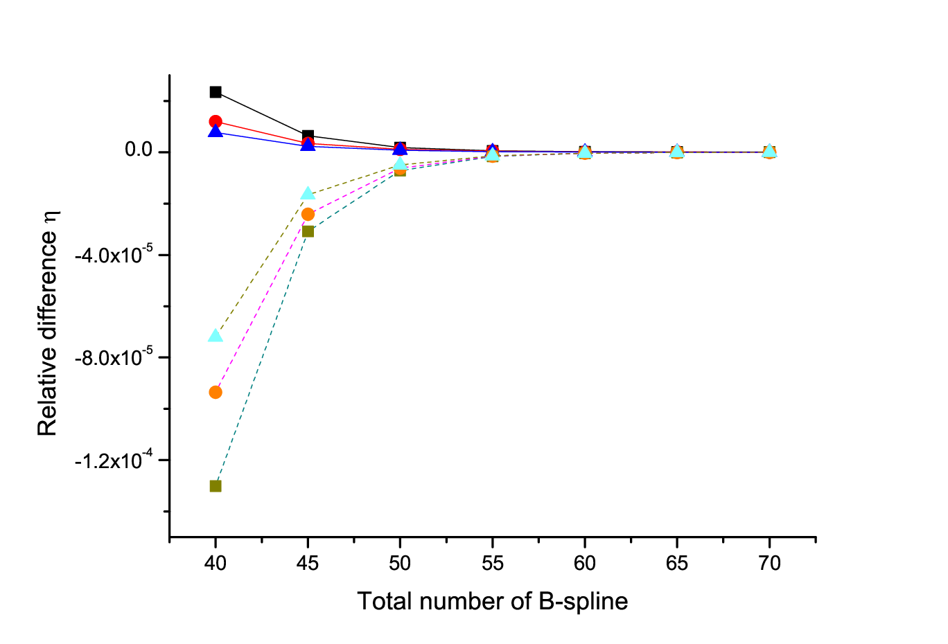
Refer to caption — Figure 1: Relative difference $\eta$ under different total number of $B$ -spline $N$ and partial-wave expansion length $l_{max}$ . The relative difference means $\eta(x)=(x-c)/c$ , where $x$ denotes our value and $c$ denotes the other high precise result. Points in solid lines and dash lines denote values in acceleration gauge and v-a gauge respectively. Square, circle and triangle points denote the results under $l_{max}=$ 2, 3 and 4 respectively.

Our results of BL in two gauges for $n\;^{1}S$ , n up to 10, states of helium are tabulated in Table 6, which also compared to the other literatures results available. In this table, our results are listed in the 2th column, the upper values in each cell are of acceleration gauge and the lower values are of v-a gauge, and so are the results of $B$ -spline basis listed in the 3th column. The values in the 5th column are truncated to 10 digits.

As shown in this table, our results in two gauges are self-consistent, having at least 7 significant digits. For $1\;^{1}S-4\;^{1}S$ states, our results in acceleration gauge are accurate to 9 significant digits, satisfied the current experimental demand. One can find that our results of the first four states remedy the inconsistencies between the results of $B$ -spline basis and the other high precise results or between the results of $B$ -spline basis in two gauges. For the $4\;^{1}S$ states, our result in acceleration gauge is in the middle of the two high precise results. Except for the $5\;^{1}S$ states, our results are consistent with these high precise results. For the $8\;^{1}S-10\;^{1}S$ states, a good agreement can be observed between our results and the results of asymptotic expansions. In our calculations, most of the knots sequence of $B$ -splines are concentrated in the first half of the box. We think further optimization of the knots sequence of $B$ -splines may be helpful to improve the accuracy of our results for higher lying, including $4\;^{1}S$ and $5\;^{1}S$ , states.

IV SUMMARY

In this article, the BL for $n\;^{1}S$ , $n$ up to 10, states of helium in acceleration gauge and velocity-acceleration gauge are calculated by using H- $B$ -spline basis set. The extrapolated results in two gauges are self-consistent and are accurate to at least 7 significant digits. In acceleration gauge, the results of BL for $1\;^{1}S-4\;^{1}S$ states are accurate to 9 significant digits. Since the H- $B$ -spline basis has capable of describing the two-electron coalescences, our results remedy the recent results of $B$ -spline basis for ${}^{1}S$ states of helium. Especial for the ground state, our result has 3 significant digits more accurate than the result of $B$ -spline basis. Our results are also compared with the other high precise results. The comparison shows a very good agreement except for $5\;^{1}S$ state. For the higher lying, including $4\;^{1}S$ and $5\;^{1}S$ , states, more precise results of using H- $B$ -spline basis might be obtained by optimizing the knots sequence of $B$ -splines.

Furthermore, to overcome the numerical linear correlation problem, we developed the MGSEPS. It is a MPI parallel program and is not limited by the computing decimal digits. This program enables us to complete our calculations and saves us lots of time. This program, we think, will bring more possibilities to precision calculations.

V ACKNOWLEDGMENTS

The authors thank Wan-Ping Zhou and Xue-Song Mei for the meaningful discussions. The numerical calculations in this article have been done on the supercomputing system in the Supercomputing Center of Wuhan University. This work is supported by the National Natural Science Foundation of China (No.11674253), (No.91536120) and (No.11504094).

Table 1: Convergence of BL for

1\;^{1}S

state of helium as total number of

B

-splines

N

increases with fixed partial-wave expansion length

l_{max}=2

r_{max}=200

and

r_{max}=400

respectively. Numbers in parentheses are computational uncertainties. Numbers in italics are invalid. Units are a.u.

N	$r_{max}=200$	$r_{max}=400$
20	4.378	4.37
25	4.371	4.369
30	4.3703	4.3705
35	4.37019	4.3702
40	4.370167	4.37017
45	4.370161	4.370164
50	4.3701599	4.370161
$\infty$	4.3701596(3)	4.370160(1)
Ref. Drake and Goldman 1999	4.370160218(3)
Ref. Yerokhin and Pachucki 2010	4.3701602229(1)
Ref. Korobov 2019	4.3701602230703(3)

Table 2: Convergence study for the ground state energy of helium as the total number of

B

-splines

N

and the partial-wave expansion length

l_{max}

increase. Numbers in parentheses are computational uncertainties. Units are a.u.

$N\backslash l_{max}$	1	2	3	4
40	-2.9035	-2.90363	-2.9036	-2.9036
45	-2.90366	-2.90369	-2.90370	-2.90371
50	-2.90370	-2.90371	-2.90371	-2.903720
55	-2.90371	-2.903721	-2.90372	-2.9037231
60	-2.903722	-2.9037231	-2.903723	-2.9037239
65	-2.9037235	-2.9037238	-2.9037241	-2.9037242
70	-2.9037239	-2.9037241	-2.9037242	-2.903724306
$\infty$				-2.90372436(6)

Table 3: Comparison of the energies for

n\;^{1}S

n

up to 10, states of helium. Numbers in parentheses of the extrapolated values are the computational uncertainties. Units are a.u.

n	${}^{1}S$	Ref. Drake 2006
1	-2.90372436(6)	-2.9037243770341195
2	-2.14597403(3)	-2.145974046054419(6)
3	-2.06127197(3)	-2.061271989740911(5)
4	-2.03358670(4)	-2.03358671703072(1)
5	-2.02117684(4)	-2.021176851574363(5)
6	-2.01456308(4)	-2.01456309844660(1)
7	-2.01062575(3)	-2.01062577621087(2)
8	-2.00809359(3)	-2.00809362210561(4)
9	-2.00636952(4)	-2.00636955310785(3)
10	-2.00514299(9)	-2.00514299174800(8)

Table 4: Convergence study of BL in acceleration gauge for the ground state of helium as the total number of

B

-splines

N

and the partial-wave expansion length

l_{max}

increase. Numbers in parentheses are computational uncertainties. Units are a.u.

$N\backslash l_{max}$	1	2	3	4
40	4.3704	4.3702	4.3702	4.37019
45	4.3690	4.37018	4.37017	4.370170
50	4.370336	4.370168	4.370165	4.370163
55	4.370330	4.370162	4.370161	4.3701613
60	4.370328	4.370161	4.3701608	4.3701606
65	4.3703275	4.3701606	4.3701604	4.3701603
70	4.3703272	4.3701604	4.3701603	4.37016027
$\infty$				4.37016022(5)

Table 5: Convergence study of BL in velocity-acceleration gauge for the ground state of helium as the total number of

B

-splines

N

and the partial-wave expansion length

l_{max}

increase. Numbers in parentheses are computational uncertainties. Units are a.u.

$N\backslash l_{max}$	1	2	3	4
40	4.369	4.3695	4.3697	4.3698
45	4.368	4.37002	4.37005	4.37008
50	4.37015	4.37012	4.37013	4.370138
55	4.370164	4.370152	4.370153	4.370154
60	4.370167	4.370158	4.3701584	4.3701585
65	4.3701682	4.370159	4.3701596	4.3701597
70	4.3701684	4.37016006	4.37016002	4.37016004
$\infty$				4.3701601(1)

Table 6: Comparison of BL for

n\;^{1}S

n

up to 10, states of helium. The upper values in each cell of the 2th and 3th column are of acceleration gauge and the lower values are of velocity-acceleration gauge respectively. Numbers in parentheses are computational uncertainties. Units are a.u.

States	this work	$B$ -spline Zhang et al. 2019	references	asymptotic expansions
$1\;^{1}S$	4.37016022(5)	4.37034(2)	4.370160218(3)^a
	4.3701601(1)	4.37014(2)	4.3701602229(1)^b
			4.3701602230703(3)^c
$2\;^{1}S$	4.36641271(1)	4.36643(1)	4.36641272(7)^a	4.366412729^d
	4.3664127(1)	4.366412(1)	4.3664127262(1)^b	4.366378229^c
			4.366412726417(1)^c
$3\;^{1}S$	4.36916480(6)	4.369170(1)	4.369164871(8)^a	4.369164888^d
	4.3691648(1)	4.3691643(2)	4.369164860824(2)^c	4.369164809^c
$4\;^{1}S$	4.36989065(5)	4.369893(1)	4.36989066(1)^a	4.369890657^d
	4.3698906(1)	4.3698903(5)	4.36989063236(1)^c	4.369890661^c
$5\;^{1}S$	4.3701520(1)	4.370152(3)	4.3701517(1)^a	4.370152093^d
	4.3701519(1)	4.3701511(2)	4.37015179631(1)^c	4.370151761^c
$6\;^{1}S$	4.370267(1)	4.37027(1)	4.37026697432(3)^c	4.370267364^d
	4.370267(1)	4.370266(2)		4.370266961^c
$7\;^{1}S$	4.370326(1)	4.37033(1)	4.37032526176(2)^c	4.370325649^d
	4.370326(1)	4.37033(1)		4.370325274^c
$8\;^{1}S$	4.370359(2)	4.37034(4)		4.370358160^d
	4.370359(2)	4.37034(2)		4.370357839^c
$9\;^{1}S$	4.370378(2)			4.370377682^d
	4.370378(2)			4.370377414^c
$10\;^{1}S$	4.370389(1)			4.370390095^d
	4.370388(1)			4.370389875^c

1

^a Drake and Goldman Drake and Goldman 1999
2

^b Yerokhin and Pachucki Yerokhin and Pachucki 2010
3

^c Korobov Korobov 2019
4

^d Drake Drake 2001

References

Pachucki et al. (2017) K. Pachucki, V. Patkóš, and V. A. Yerokhin, Physical Review A 95, 062510 (2017).
Pastor et al. (2004) P. C. Pastor, G. Giusfredi, P. D. Natale, G. Hagel, C. de Mauro, and M. Inguscio, Phys. Rev. Lett. 92, 023001 (2004).
Zheng and Sun (2017) X. Zheng and Y. Sun, Phys. Rev. Lett. 118, 063001 (2017).
Safronova et al. (2018) M. S. Safronova, D. Budker, D. DeMille, D. F. J. Kimball, A. Derevianko, and C. W. Clark, Rev. Mod. Phys. 90, 025008 (2018).
Schwartz (1964) C. Schwartz, Physical Review 134 (1964).
Wu et al. (2018) F.-F. Wu, S.-J. Yang, Y.-H. Zhang, J.-Y. Zhang, H.-X. Qiao, T.-Y. Shi, and L.-Y. Tang, Phys. Rev. A 98, 040501 (2018).
van Leeuwen and Vassen (2006) K. A. H. van Leeuwen and W. Vassen, Europhysics Letters (EPL) 76, 409 (2006).
Shiner et al. (1995) D. Shiner, R. Dixson, and V. Vedantham, Phys. Rev. Lett. 74, 3553 (1995).
Morton et al. (2006) D. C. Morton, Q. Wu, and G. W. F. Drake, Phys. Rev. A 73, 034502 (2006).
Cancio Pastor et al. (2012) P. Cancio Pastor, L. Consolino, G. Giusfredi, P. De Natale, M. Inguscio, V. A. Yerokhin, and K. Pachucki, Phys. Rev. Lett. 108, 143001 (2012).
Drake (1978) G. W. F. Drake, Physical Review A 18, 820 (1978).
Yan and Drake (1994) Z. Yan and G. W. F. Drake, Canadian Journal of Physics 72, 822 (1994).
Frolov (2000) A. M. Frolov, Physical Review E 62, 8740 (2000).
Caswell and Lepage (1986) W. E. Caswell and G. P. Lepage, Physics Letters B 167, 437 (1986).
Jentschura et al. (2005) U. D. Jentschura, A. Czarnecki, and K. Pachucki, Physical Review A 72, 062102 (2005).
Pachucki and Yerokhin (2010) K. Pachucki and V. A. Yerokhin, Physical review letters 104, 070403 (2010).
Drake and Goldman (1999) G. W. F. Drake and S. P. Goldman, Canadian Journal of Physics 77, 835 (1999).
Goldman and Drake (2000a) S. P. Goldman and G. W. F. Drake, Physical Review A 61, 052513 (2000a).
Drake (2001) G. W. F. Drake, Physica Scripta 2001, 22 (2001).
Goldman and Drake (2000b) S. P. Goldman and G. W. F. Drake, Phys. Rev. A 61, 052513 (2000b).
Korobov (2004) V. I. Korobov, Phys. Rev. A 69, 054501 (2004).
Tang et al. (2013) Y. Tang, Z. Zhong, C. Li, H. Qiao, and T. Shi, Physical Review A 87 (2013).
Zhong et al. (2013) Z.-X. Zhong, Z.-C. Yan, and T.-Y. Shi, Phys. Rev. A 88, 052520 (2013).
Schwartz (1961) C. Schwartz, Phys. Rev. 123, 1700 (1961).
Korobov (2012) V. I. Korobov, Phys. Rev. A 85, 042514 (2012).
Korobov (2019) V. I. Korobov, Phys. Rev. A 100, 012517 (2019).
Yang et al. (2017) S.-J. Yang, X.-S. Mei, T.-Y. Shi, and H.-X. Qiao, Physical Review A 95, 062505 (2017).
Bailey et al. (2002) D. H. Bailey, H. Yozo, X. S. Li, and B. Thompson, Tech. Rep., Lawrence Berkeley National Lab.(LBNL), Berkeley, CA (United States) (2002).
Zhang et al. (2019) Y.-H. Zhang, L.-J. Shen, C.-M. Xiao, J.-Y. Zhang, and T.-Y. Shi, arXiv preprint arXiv:1903.08802 (2019).
De Boor (1978) C. De Boor, Mathematics of Computation 34, 325 (1978).
Drake (2006) G. W. Drake, Springer handbook of atomic, molecular, and optical physics (Springer Science & Business Media, 2006).
Yerokhin and Pachucki (2010) V. A. Yerokhin and K. Pachucki, Phys. Rev. A 81, 022507 (2010).

Application of the Hylleraas-BB-spline basis set: Nonrelativistic Bethe logarithm of helium

Abstract

Keywords:

pacs

I INTRODUCTION

II THEORETICAL METHOD

II.1 Hylleraas-BB-spline basis set

II.2 Nonrelativistic Bethe logarithm

III RESULTS AND DISCUSSIONS

III.1 Energy Levels

III.2 Bethe Logarithm

IV SUMMARY

V ACKNOWLEDGMENTS

References

Application of the Hylleraas- $B$ -spline basis set: Nonrelativistic Bethe logarithm of helium

II.1 Hylleraas- $B$ -spline basis set