Prediction in a driven-dissipative system displaying a continuous phase transition

A subclass of driven-dissipative systems modeled by a two-dimensional cellular automaton has been proposed to understand the existence of power laws in many complex systems. Examples include the Bak-Tang-Wiesenfeld sandpile model BTW_1987, the Rundle-Jackson model Rundle_1977 and the Olami-Feder-Christensen (OFC) model OFC_1992; the latter two models have been used to gain insight into the nature of earthquakes. Many earthquake fault systems display a power-law event size distribution spanning many orders of magnitude. Such a power-law distribution is known as Gutenberg-Richter scaling in the seismology literature GR_1944. For example, the Gutenberg-Richter scaling in Southern California (1984–2000) spans about six orders of magnitude Bak_2002.

There has been a substantial interest in forecasting or predicting earthquakes. However, it has been conjectured that systems at criticality are inherently unpredictable BTW_1987. That is, events of different sizes that satisfy a scale-free distribution are due to the same physical mechanism, and thus there are no distinct precursors to distinguish one event from another Bak_1989. The idea of unpredictability at criticality has been challenged over the years. One school of thought Laherrere_1999 has proposed that very large events are due to inherently different mechanisms such as self-reinforcement, synchronization Sornette_2009 and nucleation Klein_2000, and are thus in principle distinguishable from smaller events. Some support for this proposal is the use of a technique called the log-periodic-power-law fitting procedure; it has been shown to successfully predict large, non-power law events, such as ruptures in materials Anifrani_1995; Johansen_2000 and the end of financial bubbles Feigenbaum_1996; Sornette_1996.

In this paper we address the question of predictability near and at criticality by applying machine learning to the OFC model. Previous work Pepke_1994 has shown that predictability in the OFC model decreases as the conservative limit (a critical point) is approached. We find results consistent with Ref. Pepke_1994 and investigate the predictability of events near another critical point in the OFC model: the recently observed noise transition critical point Matin_draft. By using a convolutional neural network (CNN), we find that the event sizes are more difficult to forecast as the critical point is approached and that only large events that do not satisfy power law scaling can be successfully predicted.

The Olami-Feder-Christensen (OFC) model OFC_1992 is a modified version of the spring-block model first proposed by Rundle and Jackson Rundle_1977, which is a simplification of the Burridge-Knopoff model Burridge_1967. The nearest-neighbor OFC model that we will consider consists of a two-dimensional lattice of linear dimension $L$ with each site initially assigned a random value of stress $\sigma$ between the mean residual $\sigma_{R}$ and the failure threshold $\sigma_{F}$. We denote the stress on each site, the stress grid, by the vector $\vec{\sigma}=(\sigma_{1},\ldots,\sigma_{N=L\times L})$. The system is then driven so that one site reaches $\sigma_{F}$, a procedure known as the zero velocity limit Rundle_1977. This site is said to fail, and its stress is reduced to $\sigma_{R}\pm\eta r$, where $\eta$ is the magnitude of the noise and $r$ is a uniform random variable in the range $[-1,1]$. A failing site with stress $\sigma$ distributes stress $(1-\alpha)(\sigma-\sigma_{R}\mp\eta r)/4$ to its four nearest-neighbor sites, where $\alpha$ is the dissipation parameter. The failure of one site can trigger other sites to fail, thus creating an avalanche. The avalanche or event stops when the stress of all sites is less than $\sigma_{F}$. We denote the number of failing sites, or the size of the event, by $s$. The system is then driven again using the zero velocity limit.

The OFC model is believed to approach criticality in the conservative limit $\alpha\to 0$ Christensen_1991; Serino_2001. Recently, it has been found that even for $\alpha>0$, there exists a phase transition at a critical value of the noise $\eta_{c}\approx 0.07$ Matin_draft. This phase transition is characterized by the event size distribution $n_{s}$ of the form

with

and $\tau=1.04\pm 0.14$ and $\sigma=0.43\pm 0.03$. The mean cluster size $\chi$ diverges as $(\eta-\eta_{c})_{+}^{-\gamma}$ and the connectedness length diverges as $(\eta-\eta_{c})_{+}^{-\nu}$ Stauffer_1979 with $\gamma=2.01\pm 0.14$ and $\nu=1.20\pm 0.13$, consistent with the scaling relations $\gamma=(3-\tau)/\sigma$ and $\nu=(\tau-1)/d\sigma$, where $d=2$ is the spatial dimension. Note that $n_{s}$ satisfies power law scaling for $s\lesssim s_{c}$ Matin_draft.

Our goal is to predict the event size (the number of failed sites) given the stress grid before stress has been added using the zero velocity limit and before the onset of an event. Figure 1 shows that the event size $s$ is strongly correlated with the average stress for $\eta<\eta_{c}$ and weakly correlated for $\eta\geq\eta_{c}$. The event size is weakly correlated with the variance of the stress for all values of $\eta$.

To force the CNN to learn higher order features, we first remove the correlations between the event size $s$ and the first and second moments of the stress grid. We normalize each stress grid $\vec{\sigma}$ by its average stress and the spatial variance. That is, we rescale the stress $\sigma_{i,\mu}$ at site $i$ for sample $\mu$ to $\tilde{\sigma}_{i,\mu}\equiv(\sigma_{i,\mu}-\langle{\sigma_{\mu}}\rangle)/\sqrt{\mbox{var}_{\mu}}$, where $\langle\sigma_{\mu}\rangle=1/N\sum_{i=1}^{N}\sigma_{i,\mu}$ is the mean stress per site of sample $\mu$ and $\mbox{var}_{\mu}\equiv\sum_{i=1}^{N}(\sigma_{i,\mu}-\langle\sigma_{\mu}\rangle)^{2}/N$ is the spatial variance of the stress. In the following all references to the stress will be to the rescaled stress and we will omit the tilde symbol. We will train the CNN regressor using the rescaled stress grid $\vec{\sigma}$, sampled with quasi–uniform event sizes (see the appendix).

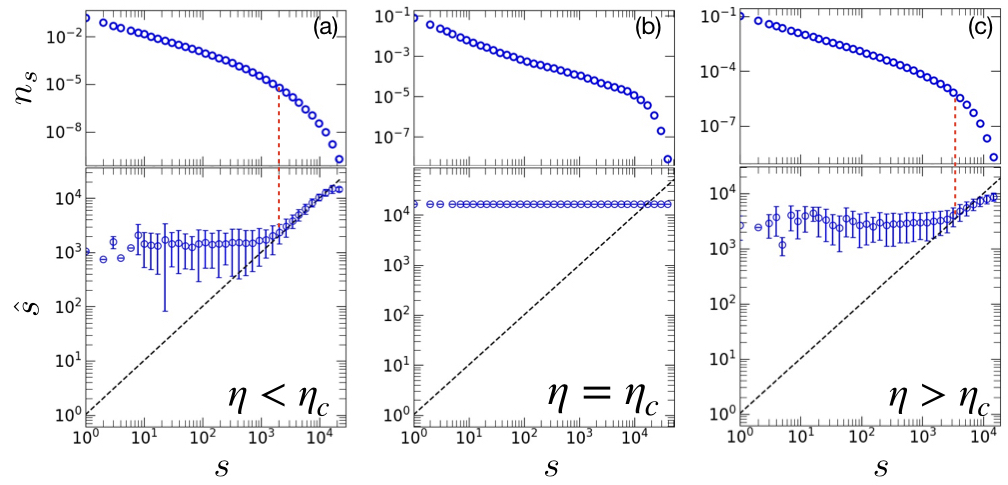
To assess the performance of the machine, we show in Fig. 2 the predicted event size $\hat{s}$ versus the true event size $s$. The top row shows the event size distribution $n_{s}$ at different values of $\eta$. The bottom row shows the predicted event sizes versus the true event sizes. We see that for $\eta<\eta_{c}$, the machine performs impressively at predicting events that are larger than $s_{c}$ [see Fig. 2(a)]. For $\eta>\eta_{c}$, the machine performs less impressively [see Fig. 2(c)]. At $\eta=\eta_{c}$, the machine fails at predicting events of all sizes [Fig. 2(b)].

In Fig. 3 we plot the testing error $\text{Err}(\log\hat{s},\,\log s)\equiv 1/N\sqrt{\sum_{i=1}^{N}(\log s_{i}-\log\hat{s}_{i})^{2}}$ as a function of $\eta$. The reason for using $\log s$ instead of $s$ in the error function is because of the larger fluctuations in $(\hat{s}-s)$ for larger $s$ and because we are interested in the relative error rather than the absolute error. The peak at $\eta_{c}$ indicates that prediction is not possible in the OFC model at criticality using only the stress grid and the CNN.

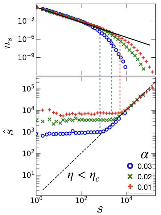
We next look at how the values of the dissipation parameter $\alpha$ affect the predictability of the system as $\alpha\to 0$. No scaling function has been found to fit the dependence of $n_{s}$ on $\alpha$ in the nearest-neighbor OFC model. Nevertheless, we can determine the cutoff $s_{c,\alpha}$ from $n_{s}$ as the value of $s$ for which $n_{s}$ deviates from a power law (see Fig. 4). As $\alpha$ decreases, the cutoff $s_{c,\alpha}$ increases. We observe that the onset of predictability is close to $s_{c,\alpha}$ and the trend persists for different values of $\alpha$.

We next explore the features that the machine has learned which allow it to successfully forecast the size of the non-scaling events and discuss why the critical events are difficult to forecast. We will use occlusion sensitivity analysis to identify the regions of importance of the images that are used by the CNN Zeiler_2014. For example, the face of a dog is expected to contain the most relevant features in determining the type of animal. Hence, blocking the face of the dog should increase the classification error of the CNN. We implement a similar analysis by defining an occluded region in the stress grid and sweeping the occluded region across the entire image to create a map that shows the regions that are the most sensitive to the occlusion. In this way we associate the region that gives the largest change in the predicted event size $\hat{s}$ with the region that is most useful in determining the size of the event.

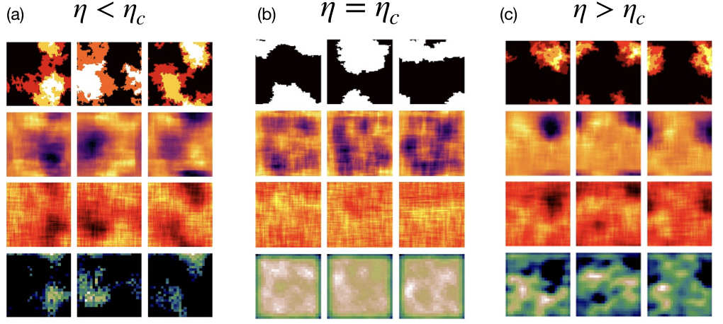
In Fig. 5 we visualize three randomly chosen samples for which $s>s_{c}$ for (a) $\eta<\eta_{c}$, (b) $\eta=\eta_{c}$, and (c) $\eta>\eta_{c}$. In the top row we show the failure maps, which correspond to the number of times that a site has failed. In the second row we show the sensitivity maps from the occlusion sensitivity analysis. Because we chose events of size $s>s_{c}$, an occlusion that yields a decrease in the predicted event size $\hat{s}$ implies a worse prediction. For $\eta\neq\eta_{c}$, the region that gives the largest decrease in $\hat{s}$ if occluded coincides with the failure region. We call the region with the largest increase in $\hat{s}$ if occluded the sensitive region. In the third row, we plot the local average stress map. To determine this map, the local average stress of a site is computed by averaging the stress of sites within a square of linear dimension $b=10$, centered at that site. Note that the region of high local stress overlaps with the failure and most sensitive regions. This consistency is reasonable because regions with high local stress have a greater probability of initiating and sustaining a large event.

Among the 32 channels in the third layer of the CNN we chose the channel that is visually the most similar to the structure of the failure region. We interpret the channel as the high level feature learned by the CNN. We plot the channels in the bottom row of Fig. 5. From these channels, we see that the machine has learned the connection between the high local stress and failure regions.

To understand why prediction is difficult at $\eta=\eta_{c}$, we look at the failure maps in the top row of Fig. 5. We see that the failure regions become more diffuse at $\eta_{c}$ compared to the more compact failure regions away from $\eta_{c}$. Although the local average stress map and the failure map remain qualitatively similar, the stress gradient between the high local stress region and the surrounding background is much smaller at $\eta=\eta_{c}$.

More quantitatively, we define a high stress region as a collection of nearest-neighbor connected sites whose local stress is above the cutoff $\overline{\sigma}_{c}$ (the bar denotes the stress is the local average stress). We measure the radius of gyration $R_{g}$ of the largest high stress region in each sample and define the density of the high stress region $\tilde{\phi}$ as the sum of the local stress within the area of radius $R_{g}$ divided by $\pi R^{2}_{g}$. The density of the high stress region $\tilde{\phi}$ decreases as $\eta_{c}$ is approached (see Fig. 6). The smaller density difference makes it more difficult for the machine to obtain the appropriate cutoff for the high stress region, thus making prediction more difficult. Multiple failures are more prominent for very large events for $\eta\neq\eta_{c}$, which is why the machine underestimates the event sizes of the very large events [Figs. 2(a) and (c)].

Since we have normalized the stress grid by the average stress before training the machine, the first and second moments of the stress grids do not contain information that can be used by the CNN to predict event sizes. The fact that the machine learns the association between the region of high local average stress and the event size means that the machine has learned the optimal cutoff that separates the high stress regions from the low stress regions. This task becomes increasingly difficult as the critical point is approached because the high stress region becomes less distinguishable from its background.

We have found evidence that events whose size distribution satisfies a power law lack distinguishable features which allow the machine to predict their size. This lack of distinguishable features is related to the difficulty of distinguishing between the fluctuations and the background at critical points Coniglio_1980. For the large non-scaling events, there exists features that allow the machine to successfully predict the event sizes. Similar conclusions are found for both the noise Matin_draft and dissipation Christensen_1991 transitions. Our results suggest that large non-scaling events are qualitatively different from the smaller scaling events. This conclusion agrees with the conjecture Bak_1989 that prediction is not possible at a true critical point ($L\to\infty$), where there is no deviation from a power law for large events.

It is known that small, large, and very large events in the long-range Rundle-Jackson model Rundle_1977 are due to different mechanisms, namely, fluctuations about the spinodal critical point, and failed nucleation and arrested nucleation events, respectively Klein_2000; Anghel_2000; Xia. These different mechanisms suggest that very large events are in principle distinguishable from other events. The caveat is that all three types of events follow a power law, albeit with different exponents. It will be interesting to see if a machine can learn the difference between the different scaling events. It is important to note that the failed and arrested nucleation events, despite the fact that they satisfy a power-law distribution, do not exhibit the same diffusive nature as the smaller events (spinodal fluctuations) on the Gutenburg-Richter scaling plot. This difference appears to be what the CNN picks up.

We would like to thank Huang Shan and Pankaj Mehta of the Department of Physics at Boston University for useful discussions.

*

References

- (1) Per Bak, Chao Tang, and Kurt Wiesenfeld, “Self-organized criticality: An explanation of the 1/f noise,” Phys. Rev. Lett. 59, 381 (1987).
- (2) John B. Rundle and David D. Jackson, “Numerical simulation of earthquake sequences,” Bulletin of the Seismological Society of America 67, 1363–1377 (1977).
- (3) Zeev Olami, Hans Jacob S. Feder, and Kim Christensen, “Self-organized criticality in a continuous, nonconservative cellular automaton modeling earthquakes,” Phys. Rev. Lett. 68 1244 (1992).
- (4) Beno Gutenberg and Charles F. Richter, “Frequency of earthquakes in California,” Bulletin of the Seismological Society of America 34, 185–188 (1944).
- (5) Per Bak, Kim Christensen, Leon Danon, and Tim Scanlon, “Unified scaling law for earthquakes,” Phys. Rev. Lett. 88, 178501, 2002.
- (6) Per Bak and Kan Chen,“The physics of fractals,” Physica D 38, 5–12 (1989.
- (7) Jean Laherrere and Didier Sornette, “Stretched exponential distributions in nature and economy: ‘fat tails’ with characteristic scales,” Eur. Phys. J. B 2, 525–539 (1998).
- (8) Didier Sornette, “Dragon-kings, black swans and the prediction of crises,” International Journal of Terraspace Science and Engineering 2, 1–18 (2009).
- (9) William Klein, Marian Anghel, C. Ferguson, John B. Rundle, and J. Sá Martins, “Statistical analysis of a model for earthquake faults with long-range stress transfer,” American Geophysical Union Geophysical Monograph Series, pp. 43–71 (2000).
- (10) J.-C. Anifrani, C. Le Floc’h, D. Sornette, and B. Souillard, “Universal log-periodic correction to renormalization group scaling for rupture stress prediction from acoustic emissions,” J. Phys. I France 5, 631–638 (1995).
- (11) Anders Johansen and Didier Sornette, “Critical ruptures,” Eur. Phys. J. B 18, 163–181 (2000).
- (12) James A. Feigenbaum and Peter G. O. Freund,“Discrete scale invariance in stock markets before crashes,”Int. J. Mod. Phys. B 10, 3737–3745 (1996).
- (13) Didier Sornette, Anders Johansen, and Jean-Philippe Bouchaud, “Stock market crashes, precursors and replicas,” J. Phys. I France 6, 167–175 (1996).
- (14) S. L. Pepke and J. M. Carlson, “Predictability of self-organizing systems,” Phys. Rev. E 5, 236 (1994).
- (15) Sakib Matin, Chon-Kit Pun, Harvey Gould, and W. Klein, “Novel effective ergodicity breaking phase transition in a driven-dissipative system,” arXiv preprint (2019).
- (16) Robert Burridge and Leon Knopoff, “Model and theoretical seismicity,” Bulletin of the Seismological Society of America 57, 341–371 (1967).
- (17) Kim Christensen and Zeev Olami, “Scaling, phase transitions, and nonuniversality in a self-organized critical cellular-automaton model,” Phys. Rev. A 46, 1829 (1992).
- (18) C. A. Serino, K. F. Tiampo, and W. Klein, “New approach to Gutenberg-Richter scaling,” Phys. Rev. Lett. 106, 108501 (2011).
- (19) Dietrich Stauffer, “Scaling theory of percolation clusters,” Physics Reports 54, 1–74 (1979).
- (20) Matthew D. Zeiler and Rob Fergus, “Visualizing and understanding convolutional networks,” European Conference on Computer Vision, pages 818–833 Springer (2014).
- (21) A. Coniglio and W. Klein, “Clusters and Ising critical droplets: a renormalisation group approach,” Journal of Physics A: Mathematical and General 13, 2775 (1980).
- (22) M. Anghel, W. Klein, J. B. Rundle, and J. S. Martins, “Scaling in a cellular automaton model of earthquake faults,” arXiv cond-mat/0002459 (2000).
- (23) J. Xia, C. A. Serino, M. Anghel, J. Tobochnik, H. Gould, W. Klein, J. B. Rundle, “Scaling behavior of the distribution of failed sites in the long-range Olami-Feder-ChristensenOlami-Feder-Christensen model of earthquakes,” manuscript in preparation.
- (24) Nitish Srivastava, Geoffrey Hinton, Alex Krizhevsky, Ilya Sutskever, and Ruslan Salakhutdinov, “Dropout: a simple way to prevent neural networks from overfitting,” The Journal of Machine Learning Research 15, 1929–1958 (2014).