Exponential suppression of bit-flips in a qubit encoded in an oscillator
Abstract
A quantum system interacts with its environment, if ever so slightly, no matter how much care is put into isolating it. As a consequence, quantum bits (qubits) undergo errors, putting dauntingly difficult constraints on the hardware suitable for quantum computation. New strategies are emerging to circumvent this problem by encoding a qubit non-locally across the phase space of a physical system. Since most sources of decoherence are due to local fluctuations, the foundational promise is to exponentially suppress errors by increasing a measure of this non-locality. Prominent examples are topological qubits which delocalize quantum information over real space and where spatial extent measures non-locality. In this work, we encode a qubit in the field quadrature space of a superconducting resonator endowed with a special mechanism that dissipates photons in pairs. This process pins down two computational states to separate locations in phase space. As we increase this separation, we measure an exponential decrease of the bit-flip rate while only linearly increasing the phase-flip rate. Since bit-flips are continuously and autonomously corrected at the single qubit level, only phase-flips are left to be corrected via a one-dimensional quantum error correction code. This exponential scaling demonstrates that resonators with non-linear dissipation are promising building blocks for universal fault-tolerant quantum computation with drastically reduced hardware overhead.
Protecting quantum states against decoherence is a fundamental problem in physics, and is pivotal for the future of quantum computing. The theory of quantum error correction (QEC) and its fault-tolerant implementation Shor1995; Steane1996 provides a solution. In QEC, groups of noisy physical qubits are arranged together to encode qubits with reduced noise, and fault-tolerance establishes that noisy quantum computers can operate reliably if the noise is below a threshold. A strong focus in quantum architecture design has been to increase this threshold to a value within experimental reach, but the required hardware overhead remains daunting Fowler2012. Therefore, there is a pressing need for new ideas to encode and protect quantum information.
Let us start by understanding why classical information is so stable. Consider a light switch, which has two stable states labeled 0 and 1. Their stability is provided by two properties. First, in order to change states one needs to apply a force to overcome an energy barrier, usually provided by the deformation of a spring. Second, friction between mechanical parts is essential for stability: when a perturbation randomly deviates the switch from its stable state, the gained entropy must be dissipated into a reservoir in order to recover the initial state. Can these two properties be transposed to protect quantum information?
The and states of a qubit, such as electronic orbitals of an ion or energy levels of a non-linear resonator, often have overlapping supports in phase space. First, one needs to isolate the two states so that they no longer overlap Fluhmann2019; Campagne2019 and separate them by an energy barrier Brooks2013; Albrecht2016; Lin2018; Earnest2018; Smith2019; Puri2017. The second property, friction (or dissipation) leaks information about the system and therefore seems incompatible with the requirement for a qubit to adopt quantum superpositions of states. Remarkably, there exists a dissipative mechanism, known as two-photon dissipation, which stabilizes the and states of a qubit without affecting quantum superpositions of the two Wolinsky1988.
Recent superconducting circuit experiments Leghtas2015; Touzard2018a have demonstrated that a resonator endowed with two-photon dissipation develops a manifold of steady states spanned by two states and , lying in two distinct locations of the resonator two-dimensional (2D) phase space. The combination of dissipation and non-locality should prevent random swaps between and (bit-flips). However, the circuit architectures mediating the two-photon dissipation impinged errors on the resonator. These experiments fell short of crossing the demanding threshold where the correction is faster than the occurrence of all errors, including those induced by the correcting mechanism itself.

In this work, we measure an exponential decrease of the bit-flip rate as we increase the separation between states and , while only linearly increasing the phase-flip rate (errors that scramble the phase of a superposition of and ). The bit-flip time reaches 1 ms, a 300-fold improvement over the energy decay time of the resonator. This was made possible by inventing a circuit which mediates a pristine non-linear coupling between the resonator and its environment, thus circumventing the problems of previous implementations Leghtas2015; Touzard2018a. Our qubit combines two unique features: only phase-flips remain to be actively corrected Guillaud2019, and its 2D phase space can be accessed to perform gates Mirrahimi2014; Grimm2019; Puri2019; Guillaud2019, making it an ideal building block for scalable fault-tolerant quantum computation with a significant reduction in hardware overhead Guillaud2019.
We follow the paradigm of cat-qubits Leghtas2013; Mirrahimi2014 where information is encoded in quantum superpositions of resonator states (see Fig. 1):
where , is a coherent state with complex amplitude , and . All these states contain an average number of photons for . A significant source of errors in a resonator is energy decay which collapses all states ( and included) towards the vacuum, thus erasing any encoded information. This decay is balanced by a mechanism where the resonator exchanges only pairs of photons with its environment (Fig. 1a) Wolinsky1988, known as two photon dissipation. This dynamics is modeled by the following loss operator
| (1) |
where is the annihilation operator of the resonator, is the rate at which pairs of photons are exchanged with the environment and the term in results from a drive which inserts pairs of photons supplement. The cat-qubit states , and all their superpositions are steady states of this dynamics. A convenient tool to visualize the semi-classical dynamics of (1) is the pseudo-potential defined over the complex plane as , where is the expectation value of at time in a semi-classical approximation supplement. Stable steady states are local minima of (see Fig. 1b) and correspond to . An error process can disrupt the stability of these states and induce transitions between them. By analogy with a particle in a double well potential, tunneling (or bit-flips) from one well to another is exponentially suppressed in the separation between the two wells (here defined as , as long as the error process fulfills two criteria: it has to be local and sufficiently weak. An error process is local if it transforms a state into neighboring states in phase space Gottesman2001. As an example, dominant errors such as photon loss, gain and dephasing are local. Moreover, the effective error rate must be weaker than the confining rate supplement inherited from the confining potential , in order for the cat-qubit states to remain localized near the potential minima. The outstanding challenge to observe an exponential increase in the bit-flip time is therefore to engineer for all dominant local error processes.

Two-photon exchange between a resonator and its environment does not occur spontaneously. Instead, it is synthesized by engineering an interaction that exchanges pairs of photons of the cat-qubit resonator with one photon of an intentionally lossy mode referred to as the buffer Leghtas2015. The interaction Hamiltonian takes the form
| (2) |
where is the annihilation operator of the buffer and is the interaction strength. Adding a resonant drive on the buffer, we recover (1) with and , where is the drive amplitude and is the buffer energy decay rate, engineered to be larger than Carmichael2007; Leghtas2015. Conveniently, the separation between the cat-qubit states is readily tunable in situ since it is proportional to the buffer drive amplitude.
We implement our cat-qubit in a circuit quantum electrodynamics architecture described in Fig 2a operated at 10 mK. It consists of a sputtered niobium film on a silicon substrate patterned into coplanar waveguide resonators. The cat-qubit mode resonates at GHz, has a single photon lifetime s and is probed through a transmon qubit coupled to a readout resonator followed by a parametric amplifier. At the flux operating point, the buffer mode resonates at GHz and has an energy decay rate MHz.

It is a technical challenge to engineer the interaction (2) without inducing spurious effects which are detrimental for the protection of quantum information. Examples of such effects are induced relaxation Sank2016; Gao2018, escape to unconfined states LescannePRApp2019 and quasiparticle generation Wang2014. To mitigate these effects, the interaction (2) is induced by a novel non-linear dipole: the Asymmetrically Threaded SQUID (ATS, Fig 2b). The ATS consists of a symmetric SQUID (Superconducting Quantum Interference Device) shunted in its center by a large inductance, thus forming two loops. Here the inductance is built from an array of 5 Josephson junctions. The ATS mediates an interaction of the form , where is the Josephson energy of the SQUID junctions, is the phase across the dipole, and are the sum and differences of flux threading the two loops supplement. We bias the ATS at , or equivalently, we thread the left and right loops with flux and , respectively. In addition, we drive the sum port with a radio-frequency flux pump . At this bias point . The ATS is coupled to the buffer and cat-qubit, so that is a linear combination of , and contains only odd powers of these operators. The desired interaction (2) is present in the expansion of , and is resonantly selected by a flux pump frequency Vrajitoarea2018. In contrast with previous strategies Leghtas2015; Touzard2018a, the ATS mediates a pristine two-photon coupling, since (2) is the only leading order non-rotating term, the presence of the inductive shunt prevents instabilities VerneyPRApp2019, and the device operates at a first order flux insensitive point (Fig 2c). These features are key in order not to introduce inherent error processes that cannot be corrected by two-photon dissipation.
The root advantage of the cat-qubit is that its computational states and can be made arbitrarily long-lived simply by increasing the cat size , provided that . In this experiment, the dominant error is due to energy decay so that kHz supplement, and with a measured kHz (from which we infer kHz). Hence, we enter the regime as soon as . We have measured that for each added photon in the cat-qubit state, the bit-flip time is multiplied by 4.2. This exponential scaling persists up to , and the bit-flip time saturates for at 1 ms, a 300-fold improvement over the resonator intrinsic lifetime (see Fig. 3). We expect a saturation when the corrected bit flip rate reaches the rate of residual errors which are not correctable, such as non-local errors. In the present experiment, we attribute this saturation to the coupling with the transmon employed for the resonator tomography supplement, which has a thermal occupation of , a lifetime s and is dispersively coupled to the cat-qubit resonator with a rate kHz. Over a timescale in the millisecond range, the transmon acquires a thermal excitation that shifts the cat-qubit resonator frequency by . This triggers a rotation of the resonator states which overcomes the confining potential since in this experiment supplement (note that tomography protocols compatible with smaller values of have been recently demonstrated Touzard2018b; Campagne2019). During an average time , the resonator states acquire an angle of order . When the transmon excitation decays, the rotation stops and the two-photon dissipation brings the resonator state back into the cat-qubit computational basis. By virtue of the dissipative nature of the protection mechanism, this process may result in a bit-flip but does not cause any leakage.

Schrödinger cat states like living in a resonator with a lifetime , lose their coherence at a rate Raimond2006. In the cat-qubit paradigm, this translates into a phase-flip rate which increases linearly with the cat size . In addition, our cat-qubit undergoes a flux pump, a drive and non-linear interactions, which could further increase the phase-flip rate. We measure the phase-flip rate for increasing and confirm a linear scaling (Fig. 4a). Moving towards three dimensional cavities and engineering ever-improving non-linear interactions should decrease the phase-flip rate below a threshold where a line repetition code can actively correct remaining errors Guillaud2019.
In conclusion, we have observed the exponential decrease of the bit-flip rate between our cat-qubit states and , as a function of their separation in phase space, while only linearly increasing their phase-flip rate. Such an exponential scaling is necessary to bridge the gap between the modest performance of quantum hardware and the exquisite performance needed for quantum computation Fowler2012. This was made possible by inventing a Josephson circuit which mediates a pristine non-linear coupling between our cat-qubit mode and its environment. Further improving the lifetime of the cavity to the state of the art of a millisecond Reagor2016 and a cat size of (resp. 10) should lead to a bit-flip time of second (resp. 0.5 hour), and a phase-flip time of s (resp. 50 s). With such a long bit-flip time, the entire effort of active QEC will be focused on correcting the only significant error: phase-flips. In addition, conditional rotations in the 2D phase space of our cat-qubit form a universal set of gates, thus bypassing the need for magic states. These features suggest a significant reduction in hardware overhead for QEC Guillaud2019.
Acknowledgements
The authors acknowledge fruitful discussions with Pierre Rouchon and Clarke Smith. ZL acknowledges support from ANR project ENDURANCE, and EMERGENCES grant ENDURANCE of Ville de Paris. AS acknowledges support from ANR project HAMROQS. The devices were fabricated within the consortium Salle Blanche Paris Centre. This work has been supported by the Paris Île-de-France Region in the framework of DIM SIRTEQ.
Author contributions
RL designed, fabricated and measured the device, and analyzed the data. RL and ZL conceived the ATS element with help from BH and TP. RL and ZL wrote the paper with input from all authors. MV fabricated the parametric amplifier. TK and MD provided experimental support. AS and MM provided theory support. ZL managed the project. All authors contributed to extensive discussions of the results.
References
- (1) P. Shor, “Scheme for reducing decoherence in quantum memory,” Phys. Rev. A, vol. 52, pp. 2493–2496, 1995.
- (2) A. Steane, “Error correcting codes in quantum theory,” Phys. Rev. Lett, vol. 77, no. 5, 1996.
- (3) A. G. Fowler, M. Mariantoni, J. M. Martinis, and A. N. Cleland, “Surface codes: Towards practical large-scale quantum computation,” Phys. Rev. A., vol. 86, p. 032324, Sept. 2012.
- (4) C. Flühmann, T. L. Nguyen, M. Marinelli, V. Negnevitsky, K. Mehta, and J. P. Home, “Encoding a qubit in a trapped-ion mechanical oscillator,” Nature, vol. 566, pp. 513–517, Feb. 2019.
- (5) P. Campagne-Ibarcq et al. 2019. In preparation.
- (6) P. Brooks, A. Kitaev, and J. Preskill, “Protected gates for superconducting qubits,” Physical Review A, vol. 87, May 2013.
- (7) S. M. Albrecht, A. P. Higginbotham, M. Madsen, F. Kuemmeth, T. S. Jespersen, J. Nygård, P. Krogstrup, and C. M. Marcus, “Exponential protection of zero modes in majorana islands,” Nature, vol. 531, pp. 206–209, Mar. 2016.
- (8) Y.-H. Lin, L. B. Nguyen, N. Grabon, J. San Miguel, N. Pankratova, and V. E. Manucharyan, “Demonstration of protection of a superconducting qubit from energy decay,” Phys. Rev. Lett., vol. 120, p. 150503, Apr 2018.
- (9) N. Earnest, S. Chakram, Y. Lu, N. Irons, R. K. Naik, N. Leung, L. Ocola, D. A. Czaplewski, B. Baker, J. Lawrence, J. Koch, and D. I. Schuster, “Realization of a system with metastable states of a capacitively shunted fluxonium,” Phys. Rev. Lett., vol. 120, p. 150504, Apr 2018.
- (10) W. C. Smith, A. Kou, X. Xiao, U. Vool, and M. H. Devoret, “Superconducting circuit protected by two-cooper-pair tunneling,” arXiv:1905.01206, 2019.
- (11) S. Puri, S. Boutin, and A. Blais, “Engineering the quantum states of light in a kerr-nonlinear resonator by two-photon driving,” npj Quantum Information, vol. 3, no. 1, p. 18, 2017.
- (12) M. Wolinsky and H. J. Carmichael, “Quantum noise in the parametric oscillator: From squeezed states to coherent-state superpositions,” Phys. Rev. Lett., vol. 60, pp. 1836–1839, May 1988.
- (13) Z. Leghtas, S. Touzard, I. M. Pop, A. Kou, B. Vlastakis, A. Petrenko, K. M. Sliwa, A. Narla, S. Shankar, M. J. Hatridge, M. Reagor, L. Frunzio, R. J. Schoelkopf, M. Mirrahimi, and M. H. Devoret, “Confining the state of light to a quantum manifold by engineered two-photon loss,” Science, vol. 347, no. 6224, pp. 853–857, 2015.
- (14) S. Touzard, A. Grimm, Z. Leghtas, S. O. Mundhada, P. Reinhold, C. Axline, M. Reagor, K. Chou, J. Blumoff, K. M. Sliwa, S. Shankar, L. Frunzio, R. J. Schoelkopf, M. Mirrahimi, and M. H. Devoret, “Coherent oscillations inside a quantum manifold stabilized by dissipation,” Phys. Rev. X, vol. 8, p. 021005, Apr 2018.
- (15) J. Guillaud and M. Mirrahimi, “Repetition cat-qubits: fault-tolerant quantum computation with highly reduced overhead,” arXiv:1904.09474, 2019.
- (16) M. Mirrahimi, Z. Leghtas, V. V. Albert, S. Touzard, R. J. Schoelkopf, L. Jiang, and M. H. Devoret, “Dynamically protected cat-qubits: a new paradigm for universal quantum computation,” New J. Phys., vol. 16, no. 4, p. 045014, 2014.
- (17) A. Grimm et al. 2019. In preparation.
- (18) S. Puri, L. St-Jean, J. A. Gross, A. Grimm, N. E. Frattini, P. S. Iyer, A. Krishna, S. Touzard, L. Jiang, A. Blais, S. T. Flammia, and S. M. Girvin, “Bias-preserving gates with stabilized cat qubits,” arXiv:1905.00450, 2019.
- (19) Z. Leghtas, G. Kirchmair, B. Vlastakis, R. J. Schoelkopf, M. H. Devoret, and M. Mirrahimi, “Hardware-Efficient Autonomous Quantum Memory Protection,” Physical Review Letters, vol. 111, p. 120501, sep 2013.
- (20) Supplementary Materials.
- (21) D. Gottesman, A. Kitaev, and J. Preskill, “Encoding a qubit in an oscillator,” Phys. Rev. A, vol. 64, p. 012310, 2001.
- (22) H. J. Carmichael, Statistical Methods in Quantum Optics 2. Springer, 2007.
- (23) D. Sank, Z. Chen, M. Khezri, J. Kelly, R. Barends, B. Campbell, Y. Chen, B. Chiaro, A. Dunsworth, A. Fowler, E. Jeffrey, E. Lucero, A. Megrant, J. Mutus, M. Neeley, C. Neill, P. J. J. O’Malley, C. Quintana, P. Roushan, A. Vainsencher, T. White, J. Wenner, A. N. Korotkov, and J. M. Martinis, “Measurement-induced state transitions in a superconducting qubit: Beyond the rotating wave approximation,” Phys. Rev. Lett., vol. 117, p. 190503, Nov 2016.
- (24) Y. Y. Gao, B. J. Lester, Y. Zhang, C. Wang, S. Rosenblum, L. Frunzio, L. Jiang, S. M. Girvin, and R. J. Schoelkopf, “Programmable interference between two microwave quantum memories,” Phys. Rev. X, vol. 8, p. 021073, Jun 2018.
- (25) R. Lescanne, L. Verney, Q. Ficheux, M. H. Devoret, B. Huard, M. Mirrahimi, and Z. Leghtas, “Escape of a driven quantum josephson circuit into unconfined states,” Phys. Rev. Applied, vol. 11, p. 014030, Jan 2019.
- (26) C. Wang, Y. Y. Gao, I. M. Pop, U. Vool, C. Axline, T. Brecht, R. W. Heeres, L. Frunzio, M. H. Devoret, G. Catelani, L. I. Glazman, and R. J. Schoelkopf, “Measurement and control of quasiparticle dynamics in a superconducting qubit,” Nature Communications, vol. 5, pp. 5836 EP –, 12 2014.
- (27) A. Vrajitoarea, Z. Huang, P. Groszkowski, J. Koch, and A. A. Houck, “Quantum control of an oscillator using stimulated nonlinearity,” 2018.
- (28) L. Verney, R. Lescanne, M. H. Devoret, Z. Leghtas, and M. Mirrahimi, “Structural instability of driven josephson circuits prevented by an inductive shunt,” Phys. Rev. Applied, vol. 11, p. 024003, Feb 2019.
- (29) S. Touzard, A. Kou, N. E. Frattini, V. V. Sivak, S. Puri, A. Grimm, L. Frunzio, S. Shankar, and M. H. Devoret, “Gated conditional displacement readout of superconducting qubits,” Phys. Rev. Lett., vol. 122, p. 080502, Feb 2019.
- (30) J. Raimond and S. Haroche, “Exploring the Quantum,” Oxford University Press, vol. 82, no. 1, p. 86, 2006.
- (31) M. Reagor, W. Pfaff, C. Axline, R. W. Heeres, N. Ofek, K. Sliwa, E. Holland, C. Wang, J. Blumoff, K. Chou, M. J. Hatridge, L. Frunzio, M. H. Devoret, L. Jiang, and R. J. Schoelkopf, “Quantum memory with millisecond coherence in circuit qed,” Phys. Rev. B, vol. 94, p. 014506, Jul 2016.
I Supplementary materials
I.1 Full device and wiring
The circuit consists of a sputtered niobium film with a thickness of 120 nm deposited on a 280 m-thick wafer of intrinsic silicon. The main circuit is etched after an optical lithography step. The Josephson junctions are made of evaporated aluminum through a PMMA/MAA resist mask patterned in a distinct e-beam lithography step. A single Dolan bridge is used to make the small junctions of the ATS and of the transmon, and a series of 3 Dolan bridges delimit the 5-junction array which serves as the ATS inductor. The full device layout and the experiment wiring are displayed in Figs. S1, S2.

I.2 Hamiltonian derivation
In this section, we derive the potential energy of the ATS dipole alone, and then calculate the full system Hamiltonian when the ATS mediates a non-linear coupling between the buffer and cat-qubit modes.
I.2.1 The potential energy of the ATS dipole element
Let us first derive the potential energy of the ATS element alone. Its equivalent circuit is represented in red in Fig. S3 and the phase across its inductor is the only degree of freedom (here we assume that the coupling capacitor to the cat-qubit mode is replaced by an open circuit). The potential energy of the ATS reads
| (S1) |
Due to fabrication imperfections, the ATS junctions are not symmetric. We introduce and such that and . We obtain
| (S2) |
where and . We DC bias the ATS at the asymmetric flux bias point (this is a saddle point of the buffer frequency map). In addition, an RF flux bias on is applied, so that
| (S3) | |||||
| (S4) |
The time-dependent potential at first order in then reads
| (S5) |
This potential is an unbounded function of , which prevents the system from escaping towards higher energy states in the presence of the pump VerneyPRApp2019_supp; LescannePRApp2019_supp. In practice, with the 5-junction array replacing the inductance, the confining part of the potential is replaced by where is the Josephson energy of each individual junction of the array. This potential is no longer unbounded, however the bound is high enough () for our pump power regime.
In the ideal case (), this potential only produces odd powers of from the sine non-linearity. A small asymmetry of the junctions produces small even powers of , leading to parasitic Kerr non-linearities. Typically . In the following we assume for simplicity.
I.2.2 The coupled buffer and cat-qubit resonators
We now consider the buffer and cat-qubit modes, and their coupling through the ATS dipole element. The full Hamiltonian reads
| (S6) | |||||
| (S7) |
where are the annihilation operators of the cat-qubit and buffer modes, their resonant frequencies, and their zero point phase fluctuations across the ATS dipole. Due to the circuit geometry, we expect . When expanding the sine up to third order in we get
| (S8) | ||||
The first two terms of the expansion are drives at frequency on the buffer and cat-qubit respectively. They can be absorbed in the frame displaced by and for and respectively, where
| (S9) |
In this displaced frame, the Hamiltonian reads
| (S10) | |||||
In practice, the buffer mode is driven with an additional microwave drive at frequency , not included here for simplicity. We place ourselves in the frame rotating at and for and respectively. In this rotated frame, the Hamiltonian reads
Performing the rotating wave approximation (RWA), we get
| (S11) |
where the modes frequencies are AC-Stark shifted to and
| (S12) |
with . When we verify the frequency matching condition
we recover Eq. (2), which we recall here
I.3 Circuit parameters
Most of the circuit parameters can be readily deduced from standard circuit-QED measurements and are gathered in Table S1. Here we explain the methodology we used to deduce the 6 dipole parameters of Fig. S3 (see Table S2) and the mapping of to . Independently of this mapping, the ATS saddle point is unambiguously found. At this flux point, , and we directly measure and . The energies and are computed from the Ambegaokar-Baratoff and the room temperature measurements of neighbouring test junction resistances. The general linear transformation mapping to is found by fitting the measured buffer frequency as a function of (see Fig. S4c,d). The impedance of the cat-qubit resonator is estimated from the aspect ratio of the coplanar waveguide geometry. The energy is adjusted to match the measured anti-crossing of the buffer and cat-qubit mode when is varied (see Fig. S4b).
|
|
|
|
| ||||||||||||||||||||||||||||||||||||||||||||||||
| ||||||||||||||||||||||||||||

I.4 Semi-classical analysis
In this section, we compute the semi-classical dynamics of the cat-qubit resonator in the presence of various imperfections (single photon loss and detuning). We gain insight into these dynamics by introducing a pseudo-potential function. For a more complete approach, we refer the reader to Refs. CohenThesis_supp; Mirrahimi2019_supp.
I.4.1 Two-photon dynamics
Under two-photon dissipation, the cat-qubit resonator state undergoes the following dynamics
| (S13) |
where the Lindblad operator is defined for any operator as . Any combination of the states is a steady state of this dynamics. Moreover, these steady states are global attractors. To gain insight, we restrict this dynamics to the set of coherent states , and introduce the pseudo-potential defined over the resonator phase space as . This pseudo-potential depicts in which direction of the phase space a coherent state evolves, and coherent steady states of the dynamics are the minima of . Following ref. Leghtas2015_supp, we have
| (S14) |
In the following we introduce and and we consider real. Separating the real and imaginary part of equation (S14), we get
The velocity of a coherent state in phase space is (see Fig. S5a,S6a). By integrating this velocity over space, we get the pseudo-potential
| (S15) |
depicted in Fig. 1b of the main text. It has two minima in and . Analyzing the evolution of small deviations and around these minima, we find
where the confinement rate is defined as
| (S16) |
This confinement pins down a computational state at each potential minimum, and protects the cat-qubit against errors. Next, we analyze the effect of errors on the cat-qubit resonator.
I.4.2 Single photon loss
When added, most Hamiltonian or dissipative mechanisms (such as detuning, single photon loss or gain, and dephasing) will perturb the system so that the two-dimensional cat-qubit space is no longer a steady-manifold of the overall dynamics. Instead, only one mixed state is a steady-state. However, this steady-state is exponentially (in ) long to reach from the cat-qubit computational states and CohenThesis_supp; Mirrahimi2019_supp. We refer to these states as metastable states. We will now use the pseudo-potential representation to visulalize the main effects of single photon loss and detuning.
Let us calculate in the presence of single photon loss at rate . The loss operator is and the overall dynamics reads
| (S17) |
Following the same computation as previously, we have
so that
| (S18) |
This velocity field is represented in Fig. S5a for and . By integrating it over space we get
| (S19) |
Cuts that pass through the two minima are plotted in Fig. S5b for various values of and .
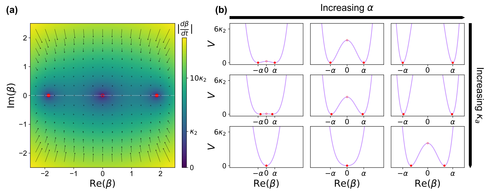
The minima of are located in with
| (S20) |
In this semi-classical analysis, we find that two metastable states form when the error rate is below the threshold
I.4.3 Detuning
In the main text, we discussed the causes of the bit-flip time saturation and blamed the random frequency shifts of the cat-qubit resonator induced by the transmon thermal excitations. Let us see how a detuning of the cat-qubit frequency affects the two-photon stabilization. In this case, we have
| (S21) |
so that
| (S22) |
Note that so we cannot perform the spatial integration to find . We can obtain the steady states directly by analyzing the velocity field (Fig. S6a) but there exists a direction in phase-space parametrized by a real parameter such that and along which the integration is meaningful. Plugging in this relation into (S22) we get the following condition on
| (S23) |
with . We have chosen the solution which approaches 0 when and for which the chosen direction crosses the steady states. Along this cut indexed by , we have
| (S24) |
leading to
| (S25) |
that is plotted in Fig. S6b. There are two minima located along the direction in
| (S26) |
In this semi-classical analysis, we find that two metastable states form provided is below the threshold
In our experiment, the detuning induced by a thermal photon entering the transmon is which is larger than for the largest .

I.5 Bit-flip time simulation
In the previous part, we gained insight on how single photon loss and detuning affect the cat-qubit protection. In the following, we perform a full master equation simulation of the system with the measured system parameters. The system consists of three relevant modes: the buffer and cat-qubit resonator, and the transmon qubit. We can write the Hamiltonian and loss operators (in the rotating frame for each mode)
| (S27) | |||||
where we have (from left to right) in the Hamiltonian, the two-to-one photon exchange factored with a drive on the buffer with strength , the Kerr of the cat-qubit, the cross-Kerr between the cat-qubit and the transmon. The two last loss operators model the decay rate of the transmon (rate ), and its thermal occupation measured to be % in the presence of the pump and drive. In order to determine the effect of the transmon on the cat-qubit, it is useful to remove the transmon from the simulation. We simulate the dynamics generated by
| (S28) | |||||
Finally by adiabatically eliminating the buffer Leghtas2015_supp we reduce to the following equivalent Hamiltonian and loss operator (provided )
| (S29) | |||||
with .
For each of these models, we numerically solve the master equation for the cat-qubit resonator prepared in state for various . By fitting the decay of to an exponential decay, we extract that we reported in Fig. S7 (full lines). For the last two models, we recover the exponential increase of the bit-flip time which scales as . The three modes model reproduces the saturation we have in the experiment and associates it with the thermal excitation of the transmon. Indeed one transmon excitation detunes the cat-qubit by which exceeds when , well above cat sizes we could achieve experimentally. In future experiment, we plan on reducing . By dividing by 10, we expect to fully circumvent this saturation (dotted lines in Fig. S7).

I.6 Tuning the cat-qubit
As explained in the main text, the flux point at which the ATS should operate is a saddle point of the buffer frequency map. It is very simple to find experimentally as we do not need to know the full mapping between , and , to recognize a saddle point. There are actually two types of saddle points as one can see on Fig. S4, the ones that are tilted to the left and the ones tilted to the right. If the two junctions forming the SQUID of the ATS were perfectly symmetric, these points would be equivalent. Otherwise, the buffer acquires a Kerr non-linearity and the two-points differ by the sign of this Kerr.
Once we find the buffer and cat-qubit frequencies we perform two-tone spectroscopy on the buffer (Fig. S8). A weak tone, referred to as the drive, probes the buffer resonance and the pump is swept in the relevant frequency range (around ). When the two-to-one exchange occurs between the buffer and the cat-qubit, we observe a sharp feature within the buffer resonance (Fig. S8a,b). The width of this feature depends on the weak tone strength and more importantly on the pump power. The pump power is pushed until before this feature becomes ill defined, when other non-linear dynamics start to play a significant role. On the cat-qubit side, within this feature the drive combined with the pump should populate the cat-qubit resonator. We check so by measuring the parity of the cat-qubit resonator and verify that it is indeed displaced. We tune the pump and buffer frequency in the middle of the displacement area (Fig. S8c). The width along of this region enables us to determine .
We perform the cat-qubit resonator full tomography after a long () pump and drive pulse (Fig. S9a) and we set the drive amplitude to produce the desired cat size (Fig. S9b). The experiment is now tuned and the cat-qubit characteristics (, time evolution of the Wigner function) can be measured.

References
- (1) Z. Leghtas, S. Touzard, I. M. Pop, A. Kou, B. Vlastakis, A. Petrenko, K. M. Sliwa, A. Narla, S. Shankar, M. J. Hatridge, M. Reagor, L. Frunzio, R. J. Schoelkopf, M. Mirrahimi, and M. H. Devoret, “Confining the state of light to a quantum manifold by engineered two-photon loss,” Science, vol. 347, no. 6224, pp. 853–857, 2015.
- (2) S. Touzard, A. Grimm, Z. Leghtas, S. O. Mundhada, P. Reinhold, C. Axline, M. Reagor, K. Chou, J. Blumoff, K. M. Sliwa, S. Shankar, L. Frunzio, R. J. Schoelkopf, M. Mirrahimi, and M. H. Devoret, “Coherent oscillations inside a quantum manifold stabilized by dissipation,” Phys. Rev. X, vol. 8, p. 021005, Apr 2018.
- (3) J. Guillaud and M. Mirrahimi, “Repetition cat-qubits: fault-tolerant quantum computation with highly reduced overhead,” arXiv:1904.09474, 2019.
- (4) M. Mirrahimi, Z. Leghtas, V. V. Albert, S. Touzard, R. J. Schoelkopf, L. Jiang, and M. H. Devoret, “Dynamically protected cat-qubits: a new paradigm for universal quantum computation,” New J. Phys., vol. 16, no. 4, p. 045014, 2014.
- (5) N. E. Frattini, V. V. Sivak, A. Lingenfelter, S. Shankar, and M. H. Devoret, “Optimizing the nonlinearity and dissipation of a snail parametric amplifier for dynamic range,” Phys. Rev. Applied, vol. 10, p. 054020, Nov 2018.
- (6) R. Lescanne, L. Verney, Q. Ficheux, M. H. Devoret, B. Huard, M. Mirrahimi, and Z. Leghtas, “Escape of a driven quantum josephson circuit into unconfined states,” Phys. Rev. Applied, vol. 11, p. 014030, Jan 2019.
- (7) L. Verney, R. Lescanne, M. H. Devoret, Z. Leghtas, and M. Mirrahimi, “Structural instability of driven josephson circuits prevented by an inductive shunt,” Phys. Rev. Applied, vol. 11, p. 024003, Feb 2019.
- (8) M. D. Reed, B. R. Johnson, A. A. Houck, L. DiCarlo, J. M. Chow, D. I. Schuster, L. Frunzio, and R. J. Schoelkopf, “Fast reset and suppressing spontaneous emission of a superconducting qubit,” Appl. Phys. Lett., vol. 96, p. 203110, May 2010.
- (9) J. Cohen, Autonomous quantum error correction with superconducting qubits. Theses, PSL Research University, Feb. 2017.
- (10) M. Mirrahimi, “Quantum error correction with cat qubits,” Les Houches Session, Quantum Information Machines, 2019.