Thermodynamics of Antiferromagnetic Solids in Magnetic Fields

The literature on the thermodynamic properties of antiferromagnets in three spatial dimensions is considerable. Low-temperature representations for the free energy density, staggered magnetization, and other observables describing quantum Heisenberg antiferromagnets have been derived, e.g., in Refs. [1, 2, 3, 4, 5, 6, 7, 8, 9, 10]. Various authors have furthermore discussed how an external magnetic field influences the low-temperature physics of antiferromagnets (see Refs. [11, 13, 12, 14, 15, 16, 17, 18]).

Due to the complexity of the problem, approximations and ad hoc assumptions are usually made within the microscopic and phenomenological approaches that the above-mentioned articles are based upon. One particularly popular method to capture the low-energy physics of antiferromagnets is the spin-wave theory, based on the fact that spin waves are the relevant low-energy degrees of freedom. The fact that these excitations are Goldstone bosons emerging due to the spontaneously broken internal symmetry O(3) $\to$ O(2), gives us, however, the opportunity to describe antiferromagnets in the systematic, model-independent language of effective field theory.

Originally, the effective Lagrangian method was developed for the spontaneously broken chiral symmetry in quantum chromodynamics that gives rise to the pions, kaons and the $\eta$-particle that constitute the corresponding Goldstone bosons: the lightest hadronic particles [19, 20]. The method, however, is universal and can be put to work whenever the phenomenon of spontaneous symmetry breaking takes place – it is perfectly suited to address condensed matter systems [21, 22], and amounts to a systematic low-energy (low-temperature) expansion of physical quantities.

Although antiferromagnets in three spatial dimensions have been analyzed with effective Lagrangians before [23, 24, 25, 26, 27, 28, 29], a systematic study of the manifestation of magnetic fields in the thermodynamic properties of the system is still lacking – both on the effective field theory and the conventional microscopic level. In particular, at the level where the spin-wave interaction becomes relevant in the thermodynamic observables, no references appear to be available. The present study hence closes a gap that has existed in the condensed-matter literature.

In a recent article, Ref. [30], antiferromagnetic films subjected to magnetic fields were studied within the effective field theory framework, and the partition function was derived up to two loops. The analogous problem for antiferromagnets that live in three spatial dimensions was solved in Ref. [31]. This task is rather nontrivial since several new issues and technical challenges regarding renormalization arise in three (as compared to two) spatial dimensions. In the present study, we take the results of Ref. [31] as a starting point to analyze a number of physical observables: pressure, staggered magnetization (the order parameter) and magnetization. We also complement the calculation done in Ref. [31] by an explicit evaluation of the magnon self-energy. This allows us to separate genuine spin-wave interaction effects from contributions due to the free gas of dressed magnons.

Overall, the effect of the spin-wave interaction that enters at the two-loop level is very small compared to the dominant contribution due to the noninteracting Bose (magnon) gas. We observe that the spin-wave interaction in the pressure can be attractive or repulsive, depending on the specific location in parameter space determined by temperature, as well as magnetic and staggered field strength. If temperature is raised from $T=0$ to a nonzero value $T$, while keeping magnetic and staggered field strengths fixed, the order parameter and the magnetization may decrease or increase as a consequence of the spin-wave interaction. Again, these subtle effects depend on temperature, as well as on the magnitude of the magnetic and staggered field.

The article is organized as follows. The two-loop representation for the free energy density is briefly reviewed in Sec. 2 to set the basis for the subsequent analysis. In Sec. 3, we then carry out the calculation of the one-loop magnon self-energies, and of the ensuing interaction part of the free energy density. (An alternative evaluation of the self-energies is given in appendix A.) Low-temperature series for the pressure, order parameter, and magnetization – in presence of magnetic and staggered fields – are derived in Sec. 4. In the same section the thermodynamic behavior of the system is discussed and illustrated using various figures. Emphasis is put on the impact of the spin-wave interaction at finite temperature. Finally, in Sec. 5 we conclude.

On the microscopic level, antiferromagnets subjected to magnetic and staggered fields are captured by the Hamiltonian

where the summation in the first term extends over nearest neighbor spin pairs on a bipartite three-dimensional lattice. The exchange constant $J<0$ defines the fundamental energy scale of the system. The first term is invariant under internal O(3) rotations, but the remaining terms that involve the magnetic field $\vec{H}$ and the staggered field $\vec{H}_{s}$, explicitly break the O(3) symmetry. Provided that these external fields are weak, the two terms represent small corrections, such that the O(3) symmetry is still approximate. This spontaneously broken approximate symmetry O(3) $\to$ O(2) is the key ingredient for the effective field theory analysis. It gives rise to the relevant low-energy excitations: the two spin-wave branches or, equivalently, the two magnon quasiparticles characterized by an energy gap.

The description of $d=3+1$¹¹ 1 Note that $d=d_{s}+1$ is the space-time dimension while $d_{s}$ stands for the spatial dimension. antiferromagnets within effective Lagrangian field theory has been discussed on various occasions and it is not our intention to be repetitive here. Rather, we refer the interested reader to Ref. [21] and sections IX-XI of Ref. [24].

We study the particular case where the magnetic field $\vec{H}$ and the staggered field $\vec{H}_{s}$ are mutually orthogonal. The coordinate frame can without loss of generality be chosen so that

The direction of the staggered magnetization order parameter in the antiferromagnetic ground state then coincides with the direction of the staggered field, and is perpendicular to the direction of the magnetic field. The dispersion relations for the two magnons take the form

where $\rho_{s}$ represents the spin stiffness and $M_{s}$ is the staggered magnetization at zero temperature and zero external fields. Remarkably, only one of the magnons “senses” the magnetic field. Due to the relativistic nature of the dispersion relations, one can identify the two magnon “masses” as

In the absence of external fields, the dispersion relations are identical: both are linear and ungapped, describing the two degenerate spin-wave branches.

The evaluation of the partition function for $d=3+1$ antiferromagnets in presence of the magnetic and staggered fields defined in Eq. (2.2), was discussed in much detail in Ref. [31]. It should be noted that in this reference, two alternative routes were pursued: a first one based on momentum-space techniques, and a second one relying one coordinate-space techniques. For technical aspects of the respective two-loop evaluations, the interested reader may consult Ref. [31]. Here we just provide the final result for the renormalized free energy density $z$, obtained within the coordinate-space approach:

The various quantities appearing therein are defined as follows. The kinematical functions $g^{I}_{r}$ and $g^{I\!I}_{r}$ describe the free Bose (magnon) gas and read

Then, the dimensionless function ${\hat{s}}$ incorporates the nontrivial part of the free energy density: the part that cannot be reduced to products of kinematical functions $g^{I}_{r}$ and $g^{I\!I}_{r}$. It is defined as

where the quantity $s$ is given by

The complicated expressions $T,U,V,W$ are defined in Eq. (B.12) of Ref. [31]. Likewise, the terms that contribute to the vacuum energy density $z^{[0]}$ – i.e., all contributions in $z$ that do not depend on temperature – are listed explicitly in Eqs. (16), (21), (50) and (51) in the same reference.

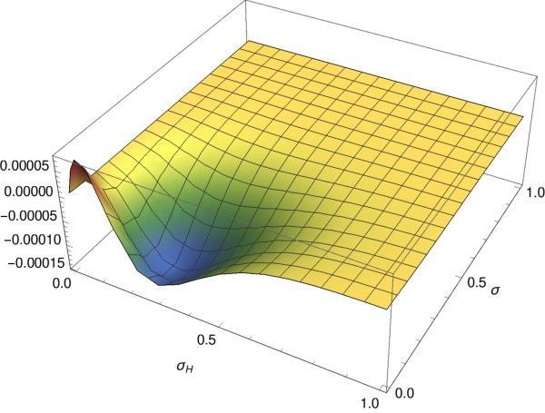
The quantity ${\hat{s}}$ really is the challenge – its numerical evaluation is described in appendix B of Ref. [31]. Here, in Fig. 1, we provide a 3D-plot of ${\hat{s}}$. Note that the function ${\hat{s}}$, much like the kinematical functions $g^{I,I\!I}_{r}$, can be expressed in terms of the dimensionless parameters $\sigma_{H}$ and $\sigma$,

These parameters measure the strength of the magnetic and the staggered fields with respect to the temperature.

Finally, the quantities ${\overline{e}_{1}},{\overline{e}_{2}},{\overline{k}_{1}},{\overline{k}_{2}}$ are the so-called renormalized next-to-leading-order (NLO) effective constants. These are pure numbers of order unity,

whose actual values depend on the renormalization scale $\mu$ via

It should be pointed out that the $\mu$-dependence of the NLO effective constants is canceled by the $\mu$-dependent logarithms in Eq. (2): indeed, the free energy density, and all thermodynamic observables derived from there, do not depend on the renormalization scale.

Naively, one might expect that the first line of our result (2) for the free energy density, that is its one-loop part, corresponds to a gas of free magnons, while all the rest captures magnon–magnon interactions. That would, however, be premature: the magnons get dressed by self-energy corrections even at $T=0$. Part of the thermal two-loop free energy density can then be accounted for as the free energy density of such dressed, yet noninteracting, magnons. Whatever is left can be considered as a genuine interaction effect.

Such a splitting of the two-loop contributions to the free energy density into free and interaction parts makes sense not only physically, but also mathematically. It will namely turn out that the interaction part of the two-loop free energy density is independent altogether of the NLO effective constants ${\overline{e}_{1}},{\overline{e}_{2}},{\overline{k}_{1}},{\overline{k}_{2}}$. By the same token, this interaction free energy density is explicitly independent of the renormalization scale $\mu$. It is, in fact, determined solely by the leading-order effective Lagrangian [31] that involves the spin stiffness $\rho_{s}$ as the only low-energy effective coupling: the question, e.g., of whether the spin-wave interaction in the pressure is attractive or repulsive, can hence be answered rigorously in a model-independent and parameter-free manner.

To see what needs to be done, consider a quasiparticle which, just like our magnons, has a relativistic dispersion relation with mass $M$, $\omega=\sqrt{\vec{k}^{2}+M^{2}}$. The complete inverse propagator for such a quasiparticle in imaginary time will take the form

where $\Pi(k_{0},\vec{k})$ is the self-energy due to quantum corrections. The exact dispersion relation of the quasiparticle is determined by the position of the pole in $\cal D$ as a function of frequency $k_{0}$. In case a mere expansion up to certain fixed order is desired, we can solve for the pole iteratively. It is then easy to see that the NLO (one-loop) self-energy $\Pi_{NLO}$ gives rise to the following “dressed” dispersion relation,

The free energy density of the noninteracting dressed magnons can now be obtained from the basic formula

Here $z^{[0]}_{free}$ is the (temperature-independent) vacuum free energy density. The leading-order dispersion relation, $\omega(\vec{k})=\sqrt{\vec{k}^{2}+M^{2}}$, gives the dominant contribution to the thermal part of the free energy density, $-\frac{1}{2}g_{0}(M)$, where the kinematical function $g_{0}$ is defined in Eq. (2.6). Let us finally expand the function $\epsilon(\vec{k})$ as²² 2 Dependence only on $\vec{k}^{2}$ follows from rotational invariance. It will be shown below that at NLO, there are no higher-order terms in the expansion in $\vec{k}^{2}$.

Expanding likewise Eq. (3.3) to first order in $\epsilon(\vec{k})$ then implies that the thermal part of the free energy density of dressed magnons to NLO is

This will be our master formula. All that is left to do is to evaluate the $T=0$ self-energies of the magnons on their “mass shell”, that is at $k_{0}^{2}=-(\vec{k}^{2}+M^{2})$.

The generic topologies of Feynman diagrams that contribute to the one-loop self-energy are shown in Fig. 2. The Feynman rules for the low-energy effective theory of antiferromagnetic spin waves were worked out in detail in Sec. 3 of Ref. [31]. The calculation itself is a matter of a simple exercise in graduate-level quantum field theory, and we therefore only quote the main results. The one-loop (imaginary-time) self-energies of the two magnons are given by

where $x$ is a Feynman parameter, $\varepsilon=2-d/2$ is the expansion parameter of dimensional regularization,

and we denoted the frequency and momentum collectively as $k$ so that $k^{2}=k_{0}^{2}+\vec{k}^{2}$. Moreover, $I_{0}$ is a zero-temperature momentum integral defined by

Finally, $a_{I,I\!I}$, $b_{I,I\!I}$, $c_{I,I\!I}$ are counterterms whose values were fixed in Ref. [31].

In the next step, we put the self-energies on the mass shell by replacing $k_{0}^{2}\to-(\vec{k}^{2}+M_{I,I\!I}^{2})$. It also proves convenient to extract the explicit dependence of the integral over the Feynman parameter on the renormalization scale. Making use of the auxiliary functions

the on-shell self-energies can be rewritten as

Note that these are linear functions of $\vec{k}^{2}$, as anticipated in Eq. (3.4). Using these expressions together with Eq. (3.5) yields the thermal free energy density of noninteracting dressed magnons. Once subtracted from the full two-loop free energy density (2), this gives the part of free energy density due to spin wave interaction. With the help of the momentum-space representation for the two-loop free energy density, developed in Ref. [31], we find

with the two-loop thermal integral

where $\vec{k}=-(\vec{p}+\vec{q})$ and we have for the sake of brevity used the shorthand notation

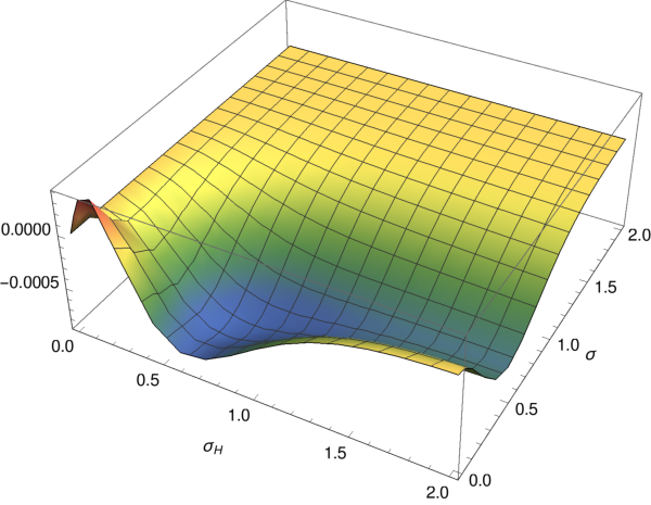
In analogy to the sunset function $\hat{s}$, Eq. (2.7), in Fig. 3 we provide a 3D-plot of the normalized two-loop thermal integral ${\cal\hat{X}}_{2}$ defined by

Eq. (3.11) is our main result, on which the following discussion of interaction effects in various physical observables is largely based. While Eq. (3.11) has been obtained within the momentum-space approach, in appendix A we derive an alternative representation for the two-loop free energy density using coordinate-space techniques.

The effective field theory expansion of the free energy density, Eq. (2), is valid at low temperatures and in weak external fields. More precisely, the quantities $T,H,H_{s}$ have to be small compared to a characteristic scale inherent in the underlying microscopic system. In the present case of the Heisenberg antiferromagnet, the thermal scale is given by the Néel temperature $T_{N}$. The actual definition of low temperature and weak field is somewhat arbitrary. To be concrete, here we choose

The question then is how $T_{N}$ is related to the exchange integral $J$ that defines the non-thermal microscopic scale. To that end we utilize the below-derived one-loop effective result, Eq. (4.12), for the order parameter $M_{s}$ as a function of temperature in the absence of external fields,

Setting $M_{s}(T)=0$, we obtain an approximate connection between $T_{N}$ and the spin stiffness,

According to Ref. [25], for the simple cubic $S=\frac{1}{2}$ antiferromagnet that we choose as a representative system, we have³³ 3 The square of the leading-order effective coupling constant $F$, used in Ref. [25], corresponds to the spin stiffness: $\rho_{s}=F^{2}$ (see Ref. [23]).

such that

To depict the low-energy behavior of the system, it is convenient to choose the dimensionless parameters $t,m_{H},m$,

These ratios are then all to be smaller than one for the effective theory to be valid, and measure the temperature and field strength with respect to the microscopic scale $J$. Of course, the actual value of $J$ depends on the specific antiferromagnetic sample. Typically, the order of magnitude of $J$ is in the meV-range (see, e.g., Ref. [32]).

Antiferromagnets subjected to magnetic and staggered fields can be addressed straightforwardly with the systematic effective Lagrangian method. Starting from the two-loop representation of the partition function, we have discussed the low-temperature behavior of $d=3+1$ antiferromagnets in a configuration of mutually orthogonal external magnetic and staggered fields.

To have a clear picture of what “interaction” means in the free energy density – and any other thermodynamic quantity derived from there – we have evaluated the self-energy of the two magnons up to one-loop order. This then allowed us to extract their dispersion relations and to rewrite the free energy density in terms of the dressed magnons. In particular, all next-to-leading-order low-energy constants (whose values are a priori unknown) can be absorbed into the dispersion relations of the dressed magnons. The remaining terms at the two-loop order then correspond to the spin-wave interaction which is fully fixed by the leading order effective constant $\rho_{s}$: the spin stiffness.

We have explored the effect of the spin-wave interaction on various thermodynamic quantities as a function of external magnetic and staggered fields. As it turns out, the interaction in the pressure is small and may be attractive or repulsive. If temperature is raised from $T=0$ to a nonzero value $T$ – while keeping the staggered and magnetic field strengths fixed – the order parameter and magnetization may decrease or increase on account of the spin-wave interaction.

References

• Oguchi [1960] T. Oguchi, Phys. Rev. 117, 117 (1960).
• Keffer and Loudon [1961] F. Keffer and R. Loudon, J. Appl. Phys. (Suppl.) 32, 2 (1961).
• Oguchi and Honma [1963] T. Oguchi and A. Honma, J. Appl. Phys. 34, 1153 (1963).
• Harris [1964] A. B. Harris, J. Appl. Phys. 35, 798 (1964).
• Lee and Liu [1967] K. H. Lee and S. H. Liu, Phys. Rev. 159, 390 (1967).
• Nagai [1969] O. Nagai, Phys. Rev. 180, 557 (1969).
• Cottam and Stinchcombe [1970] M. G. Cottam and R. B. Stinchcombe, J. Phys. C: Solid St. Phys. 3, 2326 (1970).
• Harris et al [1971] A. B. Harris, D. Kumar, B. I. Halperin, and P. C. Hohenberg, Phys. Rev. B 3, 961 (1971).
• Liu [1999] B.-G. Liu, Phys. Lett. A 259, 308 (1999).
• Hasselmann and Kopietz [2006] N. Hasselmann and P. Kopietz, Europhys. Lett. 74, 1067 (2006).
• Kaganov and Tsukernik [1958] M. I. Kaganov and V. M. Tsukernik, Sov. Phys. JETP 34, 1107 (1958).
• Falk [1964] H. Falk, Phys. Rev. 133, A1382 (1964).
• Akhiezer et al. [1961] A. I. Akhiezer, V. G. Baryakhtar, and M. I. Kaganov, Sov. Phys. Usp. 3, 567 (1961).
• Cottam and Stinchcombe [1970] M. G. Cottam and R. B. Stinchcombe, J. Phys. C: Solid St. Phys. 3, 2283 (1970).
• Fisher [1989] D. S. Fisher, Phys. Rev. B 39, 11783 (1989).
• Millan and Gottlieb [1994] C. Millán and D. Gottlieb, Phys. Rev. B 50, 242 (1994).
• Kreisel et al. [2008] A. Kreisel, F. Sauli, N. Hasselmann, and P. Kopietz, Phys. Rev. B 78, 035127 (2008).
• Neto et al. [2012] M. A. Neto, J. R. Viana, and J. R. de Sousa, J. Magn. Mag. Mat. 324, 2405 (2012).
• Gasser and Leutwyler [1984] J. Gasser and H. Leutwyler, Ann. Phys. (N.Y.) 158, 142 (1984).
• Gasser and Leutwyler [1985] J. Gasser and H. Leutwyler, Nucl. Phys. B 250, 465 (1985).
• Leutwyler [1994a] H. Leutwyler, Phys. Rev. D 49, 3033 (1994).
• Brauner et al. [2014] J. O. Andersen, T. Brauner, C. P. Hofmann, and A. Vuorinen, J. High Energy Phys. 08 (2014) 088.
• Hasenfratz and Leutwyler [1990] P. Hasenfratz and H. Leutwyler, Nucl. Phys. B 343, 241 (1990).
• Hofmann [1999] C. P. Hofmann, Phys. Rev. B 60, 388 (1999).
• Hofmann [1999] C. P. Hofmann, Phys. Rev. B 60, 406 (1999).
• Roman and Soto [1999a] J. M. Román and J. Soto, Int. J. Mod. Phys. B 13, 755 (1999).
• Roman and Soto [1999b] J. M. Román and J. Soto, Ann. Phys. 273, 37 (1999).
• Roman and Soto [2000] J. M. Román and J. Soto, Phys. Rev. B 62, 3300 (2000).
• Hofmann [2016] C. P. Hofmann, Nucl. Phys. B 916, 254 (2017).
• Hofmann [2017a] C. P. Hofmann, Phys. Rev. B 95, 134402 (2017).
• Brauner and Hofmann [2017] T. Brauner and C. P. Hofmann, Ann. Phys. 386, 178 (2017).
• Keffer [1966] F. Keffer, Spin Waves, in Encyclopedia of Physics – Ferromagnetism, edited by S. Flügge and H. P. J. Wijn (Springer, Berlin, 1966), Vol.18-2, p.1.