Fourier transform of Rauzy fractals and
point spectrum of 1D Pisot inflation tilings
Abstract.
Primitive inflation tilings of the real line with finitely many tiles of natural length and a Pisot–Vijayaraghavan unit as inflation factor are considered. We present an approach to the pure point part of their diffraction spectrum on the basis of a Fourier matrix cocycle in internal space. This cocycle leads to a transfer matrix equation and thus to a closed expression of matrix Riesz product type for the Fourier transforms of the windows for the covering model sets. In general, these windows are complicated Rauzy fractals and thus difficult to handle. Equivalently, this approach permits a construction of the (always continuously representable) eigenfunctions for the translation dynamical system induced by the inflation rule. We review and further develop the underlying theory, and illustrate it with the family of Pisa substitutions, with special emphasis on the Tribonacci case.
1. Introduction
Inflation tilings of the real line with an inflation (or stretching) factor that is a Pisot–Vijayaraghavan (PV) number are intimately related to cut and project sets. In the best case, which is the topic of the famous Pisot substitution conjecture [49, 1], their vertex points (in the geometric realisation with intervals of natural length) are regular model sets themselves, and thus have pure point spectrum, equivalently in the dynamical or in the diffraction sense [31, 8, 9]. More generally, they might have mixed spectrum, see [4, 5] and references therein for examples, but the PV-nature of still implies that they lead to Meyer sets and thus have non-trivial point spectrum [54, Sec. 5.10]; see also [53].
When analysing such inflation tilings, one quickly encounters covering model sets with complicated windows, known as Rauzy fractals [44, 42], which are compact sets of positive measure that are topologically regular (that is, they are the closure of their interior) and perfect (that is, they have no isolated points), but display a fractal boundary and often also a non-trivial fundamental group. While a lot is known about Rauzy fractals, see [48, 49, 42] and references therein, it is not obvious how to calculate their Fourier transform in closed form, which is needed to determine the diffraction intensities of the tiling system explicitly. Phrased differently, but equivalently, this Fourier transform is also needed to calculate the eigenfunctions of the corresponding dynamical system under the translation action of ; compare [32, 9].
The purpose of this contribution is to reconsider this problem in a constructive and explicit way. In particular, our goal is to make the Fourier–Bohr (FB) coefficients or amplitudes (and thus also the eigenfunctions) of such inflation tilings available, via a quadratic form with a matrix that can be expressed as an infinite matrix Riesz product. Since the latter turns out to be compactly and rapidly converging, all quantities are efficiently computable. Here, we solve the problem for inflation tilings of the real line with finitely many prototiles and an inflation factor that is a PV unit. The extension to general PV numbers and to higher dimensions will be treated separately, as this requires a bigger machinery, algebraically and analytically.
The paper is organised as follows. We begin by recalling the setting of inflation tilings of the real line in Section 2. Then, in Section 3, we introduce the Minkowski embedding and the description of our tilings (and point sets) in internal space, which leads to a contractive iterated function system for the windows of the covering model sets. This is followed by the introduction and analysis of an internal cocycle in Section 4, which leads to a matrix Riesz product expression for the Fourier transform of the Rauzy windows, and thus also for the spectral quantities we are after. In this context, in Section 5, we establish an important connection between the FB coefficients of PV inflation point sets and those of the covering model sets, which emerges through a specific uniform distribution result. Then, in Section 6, we embark on a number of illustrative examples from the family of Pisa substitutions (including some based on cubic and quartic number fields), followed by an example of covering degree in Section 7 and a brief outlook.
2. Inflation tilings of the real line
Let us begin with the symbolic side of the problem, where we consider a primitive substitution on a finite alphabet . Here, the mapping is usually specified by the -tuple . The substitution matrix of is , where counts the number of letters of type in ; see [42, 43, 6] for general background and results. We denote the characteristic polynomial of by , which is monic, but need not be irreducible over in our setting, meaning that we can also include a variety of systems with mixed spectrum.
Let be the Perron–Frobenius (PF) eigenvalue of . As is primitive by assumption, we know [24, Thm. 8.4.4] that there are strictly positive left and right eigenvectors for , denoted11 1 Since we will be using left and right eigenvectors throughout, we adopt Dirac’s bra-c-ket notation, where then stands for the sesquilinear inner product in , which becomes bilinear when restricted to . by and , which we assume to be normalised such that
Here, is the row vector with equal entries . In the substitution context, the first condition thus ensures that the entries of encode the relative letter frequencies in the symbolic sequences defined by , while the second condition implies that
| (1) |
is a projector of rank , so with , where all entries of are strictly positive. Now, let be any matrix norm, not necessarily a sub-multiplicative one, where we recall that all matrix norms are equivalent here. Then, the following property is standard; see [24, Thm. 8.5.1].
Fact 2.1.
For a primitive, non-negative matrix with PF eigenvalue , one has , where is the projector from (1). This convergence also entails that . ∎
Working with PV substitutions, we may as well profit from the underlying geometry by turning the symbolic sequences into tilings; see [52, 6] for general background and [15, 16] for the justification why this does not change the spectral type of our system. Here, we choose intervals of natural length, meaning proportional to the entries of , with control points on their left endpoints. As all entries of lie in , one normally multiplies them with their common denominator, so that they become elements of , but not of a proper, -invariant submodule. For each sequence in the symbolic hull defined by , this leads to a multi-component or typed point set, , where the emerge from the distinct types of control points and now form pairwise disjoint subsets of .
Remark 2.2.
Let us mention one consequence of the geometric setting. When with are the chosen interval lengths, the average distance between neighbouring control points in is well defined, compare [6, Sec. 4.3], and reads
so we get as the density of , and for .
Next, we invoke the set-valued displacement matrix , where the set consists of all relative (geometric) positions of tiles of type in the supertile22 2 Note that, by slight abuse of notation, we use both for the symbolic substitution and for the geometric inflation, where the meaning will always be clear from the context. ; see [3, 4, 5] for background. This gives rise to the Fourier matrix of via , so
which is a trigonometric polynomial. Since , one has the inequality
| (2) |
for all and all , where we get equality for because .
Given , we construct a cocycle (in the sense of [13, Sec. 2.1], over the dilation ) from the Fourier matrix, via
| (3) |
so together with
| (4) |
for . Inductively, one can check that is the Fourier matrix of , see [5, Fact 3.6], with . Further, one has for all , with the convention .
Recall that a matrix norm is called weakly monotone when holds for all , where denotes the matrix with entries ; see [28] for a general exposition of monotonicity properties of vector and matrix norms. With this and Eq. (2), the following property is immediate from Fact 2.1.
Fact 2.3.
The entries of the cocycle (4) satisfy , for all and all . Consequently, if is any weakly monotone matrix norm, is uniformly bounded on , which means that
is finite, with . Moreover, for all and all , one has
where the are the matrix elements of the projector from Eq. (1). This leads to more specific results on depending on the matrix norm chosen. ∎
Let us from now on assume that is a PV unit of degree . Since is an integer matrix and the equations for the left and right eigenvectors to can thus be solved in the field , a natural object to consider is the -module of rank , which satisfies . This is the main reason to choose the interval lengths for the tiling such that comprises all possible coordinates of our control points (relative to one of them, which may be placed at without loss of generality). We assume that is optimal relative to the control point set in the sense that no proper, -invariant submodule of comprises all of those points (otherwise, we change the natural interval lengths so that this is true). Next, we extract and harvest some intrinsic geometric information from this setting.
3. Minkowski embedding and internal space
Let us recall the Minkowski embedding from [6, Sec. 3.4], now tailored to . Since has degree , this will lead to a lattice as follows. There are real algebraic conjugates of , and complex conjugate pairs, so , which are defined via the irreducible, monic polynomial in that has as a root. This polynomial is a factor of the characteristic polynomial of in our case. Consequently, there are real field isomorphisms , with , and complex field isomorphisms , together with their complex conjugates, . In this setting, we can define a -linear mapping by
which extends to a -linear mapping on the field . Clearly, each image point is of the form with . The induced map is called the -map of the underlying cut and project scheme; compare [6, Sec. 7.2] or [37]. Often, only its restriction to is named the -map, but it has a unique extension to , as used here.
It is a standard result of algebraic number theory [39, Sec. I.5] that is indeed a lattice in , where we prefer the real version over the (algebraically) perhaps more natural one with because we will need Fourier transforms shortly. So, we obtain the following Euclidean cut and project scheme, or CPS for short; see [6, Sec. 7.2] and references therein for more.
| (5) |
Here, and denote the canonical projections. Such a CPS is abbreviated as .
To continue, observing that , we also need the linear mapping on that is induced by the dilation (acting on the first component) in internal space. It is immediate from the structure of and the CPS (5) that we get
| (6) |
Clearly, is a normal matrix (so, ) and a contraction, the latter because is a PV number, so all its algebraic conjugates lie strictly inside the unit disk.
Since is a -basis of , a basis matrix for can be chosen from here, with columns for . The dual matrix, , is then a basis matrix of the dual lattice,
Clearly, .
Remark 3.1.
When is minimal in the sense that the underlying point set is contained in , but not in any -invariant submodule of it, the corresponding Fourier module of the point set or tiling can be extracted from the first row of the dual basis matrix as
which is the projection of to the first component.
There is an intrinsic way to define as follows. With the Galois isomorphisms and from above, one defines the number-theoretic trace on as
| (7) |
Then, one has , which bypasses the explicit embedding step employed above, though it is of course equivalent to it.
In our setting, the Abelian group is the pure point part of the dynamical spectrum, in additive notation, for the tiling dynamical system induced by the inflation rule, where the dynamics is given by the translation action of ; see [9] for background.
To continue, in the spirit of [30], see also [6, Ch. 4], we return to the displacement matrix of . By definition, when considering the as tiles with natural length and left endpoint placed at , one has the stone inflation (compare [6, p. 148] for the concept)
More importantly, enters the induced inflation action on the point sets via the iteration
| (8) |
with a suitable and admissible initial condition, such as the left endpoints of a legal pair of intervals, one placed at and the other at the fitting position to the left. Here, we use ′ to denote the image under one iteration step. Note that this iteration produces the control point sets of the corresponding successive tile inflations. The dot indicates that the union on the right-hand side of (8) is disjoint, while stands for the Minkowski sum of point sets; compare [6, Sec. 2.1].
Remark 3.2.
Note that the iteration based on (8), viewed in the local topology, need not converge to a single typed point set . However, via a simple application of Dirichlet’s pigeon hole principle, one can show convergence to a finite cycle of such typed point sets, starting from a fixed, admissible (or legal) initial configuration. Each member of this cycle is equally well suited to define the (geometric) hull as an orbit closure under translations; compare [6, Chs. 4 and 5] for details.
Under the -map, (8) turns into an iteration of finite (and hence closed) point sets in , and thus into an iterated function system (IFS) on , where with denotes the space of non-empty, compact subsets of , equipped with the Hausdorff (metric) topology; see [10] or [49, Sec. 4.6] and references therein for background. Here, the multiplication by is replaced by the action of the contraction from (6), giving the fixed point equations
| (9) |
for . In this step, since the are compact sets in , the union on the right-hand side need no longer be disjoint. By Banach’s contraction principle, there is a unique solution to the IFS (9) within ; see [10, Thm. 1.1 and Prop. 1.3]. It is a well-known fact that the compact sets can be Rauzy fractals with complicated topological structure and boundary [48, 49]; see [42, Sec. 7.4] and references therein for background. Note that Banach’s contraction principle also gives us that each set lies dense in the set , which plays the role of a window for the CPS (5), as we shall exploit shortly.
Remark 3.3.
Let us briefly mention that Eq. (9) gives rise to a dual inflation, via multiplying from the left by , which is an expansive mapping. This results in
where . Iterating this rule in internal space either leads to a tiling or to a multiple cover of internal space, where the covering degree is constant almost everywhere. This follows from [49, Cor. 5.81], which extends an earlier idea from [27].
Next, we recall a well-known result about the solution of the IFS (9), which can be seen as a special case of [49, Prop. 4.99]. Since it is of crucial importance to our further arguments, we also include a proof that is tailored to our setting. The latter considers primitive inflation tilings of , with a PV unit as inflation factor and natural lengths of the intervals chosen such that all control point positions lie in , but in no proper, -invariant submodule of it.
Lemma 3.4.
Under our general assumptions, the solution to the IFS (9) is row-wise measure-disjoint, which means that, for each , any two distinct sets on the right-hand side of (9) intersect at most in a Lebesgue-null set.
Moreover, there is a number such that holds for all , where is the relative frequency of the tiles of type .
Proof.
All are compact sets, hence measurable, with . Let be the set of control points of type for one of the typed point sets that emerge from the limit cycle of the iteration (8), as explained in Remark 3.2. By construction, due to the properties of the -map, we then know that
where is linearly repetitive, with . Consequently, by invoking [26, Prop. 3.4], which is an extension of the density result [46, Thm. 1] for regular model sets to the more general setting of weak model sets, we know that
where refers to the (always existing) lower density of a point set. This estimate means that we have for all .
Now, due to a potential overlap of sets on the right-hand side of Eq. (9), one has
| (10) |
Observing and , this amounts to the vector inequality
where denotes the vector with entries and the inequality holds for each component. Since is the PF eigenvalue of , which is primitive, and all entries of are positive, we see that is a positive multiple of the right PF eigenvector of ; compare [47, Thm. 1.1] and its proof, which we need not repeat here.
This means we have equality in (10), which implies the first claim, while the second is a consequence of being proportional to . ∎
All mappings that occur in our IFS (9) are of the form , and hence homeomorphisms of . Invoking parts (i) and (iii) of [49, Prop. 4.99], one obtains the following improvement of Lemma 3.4.
Proposition 3.5.
Let be the unique solution to the contractive IFS (9). Then, under our assumptions, each is a perfect, topologically regular set of positive Lebesgue measure. Moreover, each boundary has Lebesgue measure . ∎
In view of this result, all are regular model sets for the cut and project scheme , see [37, 6] for background, hence also with . The corresponding dynamical system , where is the orbit closure of in the local topology and acts by translation, has pure point spectrum, both in the diffraction and in the dynamical sense; see [6, 8, 9] and references therein. The same property holds for the systems built from the translation orbit closure of any of the .
Remark 3.6.
If we consider the weighted Dirac comb with , the Bombieri–Taylor (or consistent phase) property for primitive inflation rules [5, Thm. 3.23 and Rem. 3.24] holds, which is an extension of the results of [32] to the typed point sets emerging from a primitive inflation rule. This implies the existence of coefficients , called scattering or diffraction amplitudes, such that has the diffraction measure
| (11) |
where the Fourier module is the projection of into as in Remark 3.1.
Now, assume in addition that holds for all , with the from the solution of (9). Then, due to the inflation origin, our typed point set consists of disjoint, regular model sets. Consequently, by the general theory of model sets [37, 6], the amplitudes for are given by
| (12) |
where is the characteristic function of and denotes inverse Fourier transform. For all other , one has . As we shall see later, a more general connection is possible via the FB coefficients of and its subsets; see Eq. (19) below for more. Note that the validity of (12) is a consequence of the uniform distribution of in ; compare the detailed discussions in [6, Sec. 7.1] and [46, 38].
Though Eq. (12) looks nice, it is generally difficult to calculate directly, due to the potentially fractal nature of the window boundaries. Let us thus turn to an alternative approach of transfer matrix type that harvests the inflation nature of our point sets. In view of Lemma 3.4, Eq. (9) can now be rewritten as
| (13) |
to be understood in the Lebesgue sense (rather than pointwise).
Theorem 3.7.
Let be the unique solution to the contractive IFS (9). Then, Eq. (13) holds in the Lebesgue sense for every .
Moreover, when considering the compact set , one has
where is a measurable, integer-valued function on with . In particular, the potential values on are restricted to .
Proof.
Since all are compact, the function is well defined for all , and clearly outside of . This means that we have on all of , while all remaining claims of the theorem are now immediate. ∎
Remark 3.8.
Under some additional conditions, the function is constant for almost every , with integer value . In this case, one has . This situation happens whenever the inflation defines a model set, where . Beyond this case, one can have integer values of , possibly up to .
In general, however, the function need not be constant almost everywhere in the total window , as we shall see in the example of Eq. (24) in Section 7. This seems a significant difference to the covering degree of internal space by the dual inflation mentioned in Remark 3.3. We shall return to this point in Section 5.
Let us now switch to an analysis of the system (13) of equations after (inverse) Fourier transform, which turns it into a rescaling equation for an -tuple of continuous functions.
4. Analysis of internal cocycle
Let us first recall a simple, but in our context vital, result on the inverse Fourier transform of characteristic functions, which we prove for convenience.
Lemma 4.1.
Let be fixed. Let be compact and . Then, one has the relation
which holds for all , with continuity in both variables.
Proof.
With the change of variable , one finds
Continuity in follows from the Fourier transform of an -function being continuous, see [45, Thm. IX.7], while continuity in is obvious. ∎
Let now be the linear map from (6) in internal space that is induced by the dilation in direct space, . Set and consider the vector of functions . Also, let be the internal Fourier matrix that emerges from the (inverse) Fourier transform of the -image of the displacement matrix , that is,
with . The matrix elements are again trigonometric polynomials, this time generally multivariate, where one still has
for all and all , in complete analogy to (2). With Lemma 4.1 and , one now finds the following result of transfer matrix type via an elementary computation; compare [41, Sec. 3.2] for a mathematically similar structure.
Proposition 4.2.
It is clear that . Moreover, from the way it was constructed, we know that is a normal matrix and a contraction. Consequently, its spectral norm agrees with its spectral radius, see [25, Sec. 2.3], and we have . This leads to the following property, where we use also for the -norm of vectors.
Lemma 4.3.
For any , there exists such that
holds simultaneously for all and all .
Proof.
Recall that holds for all . Observe that
where we have used some trigonometric identities and the fact that holds for all . Combining this with the Cauchy–Schwarz inequality
gives the claim by standard arguments. ∎
Now, for , we can define an internal cocycle from the Fourier matrix via
with and . In analogy to (4), we now have
| (14) |
for all , and also for all and , the latter with the convention , which we adopt from now on. Clearly, one has , and Fact 2.3 remains valid with replaced by the internal cocycle .
Next, we want to consider the matrix function defined by
| (15) |
with , where because is a unit. We thus need to establish that is well defined as a limit, for every . To this end, we employ the -norm for vectors and the corresponding operator norm, both denoted by as before.
Proposition 4.4.
The sequence of matrix functions is equicontinuous at , which is to say that
Proof.
Since is non-negative, the spectral radius of is , for all . Let us first consider the case that is normal. Then, we can most easily work with the spectral norm, because we have for , hence . Also, we get
for all in this case. This estimate holds because the spectral norm has the required monotonicity property; compare [28, Thm. 1] or [24, Exc. 5.6.P42].
Now, harvesting the cocycle property (14), a simple telescopic argument leads to
for , with as above. Via the triangle inequality, using the above properties, one then finds the estimate
For and , with and the from Lemma 4.3, this gives
by a geometric series argument, which establishes the claim when is normal.
For the general case, we employ a different sub-multiplicative matrix norm, which depends on and again satisfies , hence . Following [25, Sec. 2.4], one such norm can simply be constructed as follows. Consider the convex body
where the are the strictly positive entries of , the (frequency normalised) right PF eigenvector of , and define
This is a matrix norm on that is absolute, so for all , with denoting the vector with entries . Now, let denote the matching operator norm on , as defined by
which is sub-multiplicative and satisfies by construction. What is more, it also satisfies the monotonicity property for all , again by [24, Thm. 1]. Consequently, we still get for all and all .
Equipped with this matrix norm, we can repeat our previous telescopic argument, now leading to the estimate
From here, since the vector norms and are equivalent, as are the matrix norms and , we can adjust the choice of to reach the same conclusion. ∎
Combining the equicontinuity of at from Proposition 4.4 with and Fact 2.1, a standard -argument gives the following consequence.
Corollary 4.5.
Let be the projector from (1) and the internal cocycle. Then, for all , there exists and such that
holds for all integer and all with . ∎
Now, we are set to establish the convergence of our internal cocycle as follows.
Theorem 4.6.
The scaled internal cocycle sequence converges compactly on . Consequently, the matrix function from (15) is well defined and continuous.
Proof.
Let be compact, choose , and let be as in Proposition 4.4. We will establish the claim by showing that the sequence is uniformly Cauchy on .
For , we employ the cocycle property from (14) to get
| (16) |
where the first factor on the right is bounded by and thus uniformly bounded by a constant , as a consequence of Fact 2.3, applied to with the spectral norm. Via the triangle inequality, the second factor on the right-hand side of (16) is bounded by
| (17) |
Choose large enough so that is contained in the open ball of radius around , which is possible because is a contraction. Then, the first term in (17), as well as the last, is bounded by . Since converges to by Fact 2.1, where , the sequence is Cauchy, so there is a such that the middle term in (17) is bounded by , for all and . Consequently, (17) is bounded by for the chosen , all , and all . Via Fact 2.3, used with instead of , this gives an upper bound of to the left-hand side of (16). As this bound is independent of , and was arbitrary, uniform convergence on follows.
Since we have a compactly convergent sequence of matrix functions, each of which is analytic and thus certainly continuous, the last claim is obvious. ∎
Let us next analyse the matrix function , where we know
from Fact 2.1. Now, Eq. (14) implies that, for any fixed ,
because is a contraction and . With , this gives
as well as from taking the limit . Each row of thus is a left eigenvector of for its eigenvalue , or vanishes, hence is a -dependent multiple of . But this means
| (18) |
with . Observing that the window volumes are proportional to the entries of by Lemma 3.4, so for some , one has the following consequence.
Corollary 4.7.
In particular, this result makes the functions effectively computable from .
Remark 4.8.
Let us mention that the continuity of the functions is also clear from the fact that each is the (inverse) Fourier transform of an -function, and decays at infinity by the Riemann–Lebesgue lemma; see [45, Thm. IX.7]. What is more, since all are compact, we actually know that each has an analytic continuation to an entire analytic function of variables, with a well-known growth estimate according to the Paley–Wiener theorem; see [45, Thm. IX.12]. This also means that the rank of is almost everywhere.
5. Fourier–Bohr coefficients and uniform distribution
Here, we explain the general connection with the diffraction amplitudes mentioned earlier in Remark 3.6. Given a typed point set , its Fourier–Bohr (FB) coefficient (or amplitude) at is defined as a volume-averaged exponential sum,
| (19) |
and similarly for the control point sets with , provided the limits exist. This is the case for point sets from primitive inflation rules, which are linearly repetitive and thus uniquely ergodic [52, 29]. The definition entails that , and one gets for all because the point sets are disjoint by construction. Let us also recall that , when viewed as a function of , is continuous, which correponds to the continuity of all eigenfunctions in this setting [32]; see Remark 5.6 below for more.
In general, we know from the embedding procedure that . If is also a model set, the point set is uniformly distributed (and even well distributed) in ; compare [46, 38]. This uniform distribution occurs more generally, as we analyse next.
It is clear from Remark 3.8 and the example in Section 7 that the lift of to internal space will not be uniformly distributed in in general. However, the situation is more favourable for the individual point sets . For any , consider the sequence of point measures in internal space defined by
Clearly, one has by construction, and exists (under weak convergence), due to the strict ergodicity of the dynamical system defined by . An explicit argument for this convergence, based on the linear repetitivity of , can be formulated along the lines of the proof of [29, Thm. 5.1], observing that and using the result pointwise. Here, is a positive measure on with and total mass . We say that induces the measure in internal space.
Remark 5.1.
If and with , one can consider, for each fixed ,
Now, since any is bounded, the Delone property of implies that there are some numbers such that implies
and each is a local weight function in the sense of [29].
Then, [29, Thm. 5.1] yields convergence of , uniformly in , due to the linear repetitivity of the . An analogous argument applies when is replaced by with an arbitrary . The result obtained this way is stronger than needed below, and actually also gives the uniform existence of the FB coefficients.
When induces , a simple calculation (with a change of the summation variable) shows that with induces the positive measure
where is the contraction from (6) and denotes the push-forward of a finite measure , so for . Equivalently, one can use with an arbitrary Borel set.
Let us now assume that our typed point set is a fixed point of the inflation equation (8). This is no restriction as one can always achieve this via replacing by a suitable power; compare Remark 3.2. Then, our induced measures must satisfy
| (20) |
which defines a system of linear equations. We can spell out one solution as follows, where denotes Lebesgue measure on internal space, .
Lemma 5.2.
Proof.
Observe that , which follows from a simple change of variable calculation. Likewise, one has , and inserting the expressions into (20) leads to
By construction, we have , where is the relative frequency of points of type ; compare Remark 2.2. On the other hand, we know from Lemma 3.4 that the window volumes satisfy for some fixed , which implies that
is independent of , and the previous equation turns into the window equation (13), which is satisfied in the Lebesgue sense.
The claimed normalisation is obvious. ∎
Now, we interpret the right-hand side of (20) as a linear mapping on , with denoting the finite, positive measures on , equipped with the total variation norm, . If is an -tuple of positive measures, its image is with
Consequently, when for all and some , the total mass of each is preserved under the iteration because . This leads to the following result.
Proposition 5.3.
Proof.
The space can be equipped with the Hutchinson metric, compare [10, Sec. 2] and references therein, which turns it into a complete metric space. The iteration then is a contraction, as is obvious from
where ; see [10, Sec. 5] for the remaining steps.
Now, the first claim is a consequence of Banach’s contraction principle, while the concrete form of the solution follows from Lemma 5.2. ∎
If one starts the iteration with an arbitrary -tuple of non-negative measures, not all , there is a unique component of the total mass vector in the PF direction of , which defines the parameter , and all other components decay exponentially fast.
Our main result of this section can now be formulated as follows.
Theorem 5.4.
Let be the typed point set of a primitive, unimodular PV inflation rule as constructed above, and consider the natural CPS that emerges from the Minkowski embedding. Then, each induces a unique measure in internal space, namely
where the are the solutions of the window IFS (9). This entails the statement that, for all , the set is uniformly distributed in .
Proof.
The IFS (20) for the distributions induced by the on the compact sets is contractive on , with , and the unique solution is the one stated.
Recalling the definition of the induced measures, weak convergence clearly is equivalent to the uniform distribution of in . ∎
At this point, we can return to the connection between the FB coefficients and the Fourier transform of the windows, even though the latter generally only code a covering model set. Still, due to uniform distribution, one obtains an explicit formula as follows.
Corollary 5.5.
Under the assumptions of Theorem 5.4, the FB coefficients of the are proportional to the Fourier amplitudes of the covering model set via
for any , together with for any . ∎
In the special situation that the function from Remark 3.8 satisfies for a.e. , one further gets
| (21) |
which reduces to the standard formula for model sets when .
Remark 5.6.
If we interpret the FB coefficient as a function of , one obtains
Consequently, whenever the coefficient does not vanish, this defines an eigenfunction of the strictly ergodic dynamical system , where is the hull of obtained as the closure of the translation orbit in the local topology; compare [6, Ch. 4]. The analogous connection exists with the for , not all of which can vanish simultaneously for any given . This explains why is the pure point part of the dynamical spectrum (in additive notation) and how the diffraction intensities are connected with the eigenfunctions; see [9, 32] and references therein for more.
Both for regular model sets and for primitive inflation tilings, it is known that the eigenfunctions on have continuous representatives; see [32] and references therein. This also means that the dynamical point spectrum for such systems is the same in the topological and in the measure-theoretic sense.
Whenever constant covering of the total window is satisfied in our setting, we have the following consequence for the FB coefficients, where we use from (18) and Corollary 4.7.
Corollary 5.7.
Assume that the total window covering is almost surely constant. Then, the FB coefficients, for , are obtained as
and vanish for all other .∎
The corresponding diffraction intensities follow from Eq. (11). Note that the covering degree does not show up in this relation. The intensity at any wave number can efficiently be approximated by truncating the infinite product representation for and calculating the amplitudes as explained above.
At this point, we turn to some applications of the cocycle method to concrete inflation systems on the real line, which will illustrate the above results.
6. Examples – the Pisa substitutions
Let us introduce an interesting family of primitive inflations as follows, based on the alphabet with . The explicit rule is given by for , together with . In short, we have . We call the family of Pisa substitutions. For , this is the classic Fibonacci rule, while is known as the Tribonacci substitution in the literature; see [42] and references therein.
Let us first collect some general results for this family. The substitution matrix reads
with . Note that is not normal for , whence we need Proposition 4.4 in the generality stated and proved. The characteristic polynomial of is
By [14, Thm. 2], is irreducible, with one root , which is the PF eigenvalue of , and all others inside the unit disk. So, is a PV unit of degree , which satisfies . The discriminant of for is given by
which is due to M. Alekseyev; see [51, A106273] for details.
The right PF eigenvector is denoted by as before, where we now drop the dependence on for ease of notation. When normalised as , it reads
The corresponding left PF eigenvector is normalised such that , which gives
Here, the normalisation prefactor was simplified via the algebraic relation for from , which in particular gives . Note that the vector on the right-hand side is a canonical choice for the natural interval lengths, which all lie in . The shortest interval then has length , and it is straightforward to show that no proper, -invariant submodule of contains all control point positions. Here, the density of the resulting point set is
with .
When working with the -module , one can define the dual module with respect to the quadratic form as explained in Remark 3.1, namely
| (22) |
For our family, one finds with
We are now set to look at some special cases in more detail.
6.1. The Fibonacci tiling
For , which we write with the binary alphabet for simplicity, the inflation tiling with interval lengths for and for is well studied; see [6, Sec. 9.4.1] and references therein. For the standard fixed point of the square of , with central seed , one obtains the windows and , compare [6, Ex. 7.3], and can calculate their Fourier transforms immediately. With , they read
Here, it does not matter whether we take open, half-open or closed intervals, as their characteristic functions are equal as -functions. Consequently, this detail is spectrally invisible.
The internal Fourier matrix and cocycle for this example read
with33 3 Here, is a number which should not be confused with the Galois isomorphisms from Section 3. , so . We find the relation
expressing in terms of , while the latter is obtained as the limit
where the trigonometric polynomials are recursively defined by
with initial conditions . From here, it is not difficult to check that
as it must. The convergence of the recursive formula for is exponentially fast. Though there is no need for this alternative approach in this case, it provides a consistency check and some additional insight into the recursive structure of the spectrum.
6.2. (Twisted) Tribonacci
Here, we compare two different substitution rules for , which share the same substitution matrix, . These are the Tribonacci substitution and its twisted counterpart, , with the alphabet . Further permutations of letter positions do not define new hulls, as they are conjugate to one of these two. Both lead to inflation systems with fractal windows in their model set description, as they must due to a result by Pleasants [40, Prop. 2.35], but the twisted version is more tortuous; see Figure 1 below, and compare [42, Figs. 7.5 and 7.8], where a different coordinate system is used. The fundamental group of the windows in the twisted case is huge, while the windows of the untwisted case are still simply connected, as in other examples such as the inflation tiling that underlies the Kolakoski- sequence [11].
The field is cubic. For ease of notation, we define . With this, we find that the PF eigenvalue is
The characteristic polynomial is cubic, , with discriminant . The remaining two eigenvalues form a complex conjugate pair with , where we assume to be the one with positive imaginary part. One also has . Further, one finds and , while and . From the discriminant and Vieta’s theorem, one also gets
The natural tile lengths can be chosen as , which means that all control point positions lie in the rank- -module , but in no proper submodule. The lattice for the CPS, , is obtained from the Minkowski embedding of into -space. A canonical choice for the basis matrix of and its dual, , is then given by
with . From the first row of , one can now extract the Fourier module in our setting from an independent calculation, which gives
with , in agreement with our general formula (22). The Abelian group is also the dynamical spectrum (in additive notation) of our systems; compare Remark 3.1. In fact, Tribonacci and twisted Tribonacci are metrically isomorphic by the Halmos–von Neumann theorem, but have rather different eigenfunctions. Also, they are obviously not mutually locally derivable (MLD) from one another; see [6, Sec. 5.2] for background. Moreover, they are not topologically conjugate either, as they can be distinguished via invariants of gauge-theoretic origin [22], or by dimension arguments as follows.

Remark 6.1.
The Hausdorff dimension of the fractal boundary of the Tribonacci windows is known; compare [36] as well as [18, Ex. 4.2]. It can be calculated as a similarity dimension, which is the real solution to the equation . This gives
where is the positive real root of .
Likewise, for twisted Tribonacci, the Hausdorff dimension of the window boundary is given by [18, Ex. 4.3]
where now is the positive real root of , as one derives from the corresponding graph-directed IFS for the boundary; see also [49, Sec. 6.9].
The much larger Hausdorff dimension for the twisted case corresponds to a slower decay of the Fourier transform; see [33, App. B] for an explicit one-dimensional example for which the Fourier transform shows a power-law decay with exponent , where is the fractal dimension of the boundary, and [23] for an interesting asymptotic scaling analysis of such coefficients. It would be useful to establish a general result along these lines, which is of recent interest also with respect to a refinement of the notion of complexity [21].
If is the field isomorphism induced by , one determines the -map of as . For , this gives
where the integers are known as the Miller indices of the corresponding Bragg peak in crystallography.

In Figure 2, we compare the peaks of the pure point diffraction measure for the Tribonacci point set and its twisted sibling. The support is the same, but the intensities show characteristic differences. The latter are calculated as
with the appropriate matrix function for the two cases. The peaks of the twisted case are often smaller than their untwisted counterparts. Note also that an approximation of the diffraction measure by exponential sums of large patches suffers from slow convergence, in particular for the twisted version, as was previously observed and discussed for the plastic number PV inflation [7]. This reference also contains an illustration of the full Fourier transform of the plastic number Rauzy fractal, which shows similar features as our case at hand.
6.3. The quartic case
Let us briefly consider on , where is a quartic field. Beyond the PF eigenvalue , has one real root , with , and a complex conjugate pair , with . For the natural choice of interval lengths, , the Fourier module becomes
where
This follows from (22) and can be verified via the quadratic form , observing and for . In analogy to before, we parametrise by a quadruple of Miller indices.
The internal Fourier matrix reads
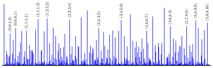
with . A calculation analogous to our previous ones leads to the diffraction measure as illustrated in Figure 3. Let us briefly mention that, using the methods from [49, Cor. 4.118 and Prop. 4.122], one can derive an upper bound of for the Hausdorff dimension of the window boundaries [50]. It is no problem to twist , as we did for the Tribonacci case, but we leave further details to the interested reader.
7. Twisted extensions of Fibonacci chains with mixed spectrum
Let us close with a simple system with mixed spectrum. It is based on the idea, taken from [4], of a twisted extension of , which is from Section 6.1, with a bar swap symmetry. As such, it works with the extended alphabet , where we consider
The natural interval lengths are those of the Fibonacci tiling, so for and , as well as for and . Also, by identifying with and with , one sees that the system possesses the Fibonacci tiling as a topological factor, where the factor map is almost everywhere, but not everywhere [22]. Consequently, we have a non-trivial point spectrum, together with a continuous component. The latter, by an application of the renormalisation methods from [5, 34, 35], must be singular continuous.
The substitution matrix of has spectrum , and a reducible characteristic polynomial. Only the factor with as a root is relevant, and one checks that the same embedding as for the Fibonacci tiling can be used. Here, the embedding method produces covering supersets, where the contractive IFS on reads
with as before. The unique solution with compact subsets of is
| (23) |
as can easily be verified by direct computation. Here, we are in the situation that for a.e. , and uniform distribution is preserved both in the individual windows, by Theorem 5.4, and in the total window.
Note that the point sets and are disjoint, but have the same closure, and analogously for and . The right-hand sides of the window equations are measure-disjoint by Lemma 3.4, which means that the cocycle approach can be applied, with the window covering degree being . Since uniform distribution is satisfied here by Theorem 5.4, the FB coefficients from (19) can be calculated by means of (21). For weights with , the pure point part of the diffraction reads
with the additional part of the diffraction measure being singular continuous.
As was noticed by Gähler [22], one can employ a partial return word coding to arrive at another inflation which defines a tiling system that is MLD with the above. Concretely, consider the alphabet and the inflation . Here, and correspond to and , while replaces and replaces each that is not followed by a . This gives the substitution matrix
with the same eigenvalues as above. The natural interval lengths are , in agreement with the local derivation rule just stated.
The resulting window equations read
which constitute a contractive IFS on with unique solution
The total window is as in the twisted Fibonacci example, but the window function now is a step function as induced by
| (24) | ![[Uncaptioned image]](1907.11012v2/returnwin.png) |
As was further analysed by Gähler [22], there is also a maximal topological pure point factor such that the factor map is 2 :1 everywhere. Using the alphabet , this maximal pure point factor is given by the inflation rule
where and stand for intervals of length , while those of type and have unit length. The factor map can most easily be given as a block map, where words of length at position are mapped to an element of the new alphabet at the same position, namely
| (25) |
and correspondingly for the tilings, where the resulting mapping is called a local derivation rule; see [6, Sec. 5.2] for details.

Conversely, one proceeds in two steps. First, any given sequence from the (symbolic) hull of is mapped to a sequence in by and . In the second step, choose one position and decide whether to place a bar on the letter or not. Then, the bar status of the two neighbouring symbols is uniquely determined from the original block map (25), read backwards. Inductively, this fixes the entire sequence. Since the only choice was the initial bar, this shows that the block map (25) is globally 2 :1. Once again, this block map transfers to a local derivation rule for the corresponding tilings.
The new inflation rule leads to a regular model set, with window equations
Due to the factor map, we immediately know that and with and from (23). The unique solution can be determined by first observing that each with can be expressed in terms of . This gives a rescaling equation for alone, namely
where and .
This leads to which results in the formula
| (26) |
while the other windows follow from here via affine mappings. All four windows are illustrated in Figure 4, each comprising countably many disjoint intervals.
The explicit expression for in (26) leads to the (inverse) Fourier transform of its characteristic function in the form
| (27) |
with , which is the total length of the window ; see Figure 5 for a comparison of with the function .

For the cocycle approach, we first note that the internal Fourier matrix reads
with as usual. The frequency-normalised right PF eigenvector is
where one has for the total window lengths. With , one gets , where the convergence of the underlying matrix product is exponentially fast. Here, one can then study the rate of convergence in comparison to the alternative formula in (27).
8. Outlook
It is possible to extend our approach to inflation tilings in higher dimensions, if the inflation multiplier is a PV unit. In fact, this is needed and useful when dealing with direct product variations (DPV) as considered in [19, 20, 2].
An extension to the non-unit case is also possible, but requires a larger machinery from algebraic number theory, as developed in [49] for the treatment of the Pisot substitution conjecture in the general non-unit case. This is work in progress.
Finally, also -adic type inflations can be covered, provided that the participating inflation rules are compatible in the sense that they share the same substitution matrix. Further, there are applications of our results to the Eberlein decomposition for Dirac combs of primitive inflation systems [12] and consequences for the spectral theory of regular sequences [17].
Acknowledgements
It is a pleasure to thank N.P. Frank, F. Gähler, N. Mañibo, B. Sing and N. Strungaru for helpful discussions, and an anonymous referee for several thoughtful suggestions that helped to improve the presentation. Our work was supported by the German Research Foundation (DFG), within the CRC 1283 at Bielefeld University, and by EPSRC through grant EP/S010335/1.
References
- [1] Akiyama S, Barge M, Berthé V, Lee J-Y and Siegel A, On the Pisot substitution conjecture, in Mathematics of Aperiodic Order, eds. Kellendonk J, Lenz D and Savinien J, Birkhäuser, Basel (2015), pp. 33–72.
- [2] Baake M, Frank N P and Grimm U, Three variations on a theme by Fibonacci, Stoch. Dyn. 21 (2021) 2140001:1–23; arXiv:1910.00988.
- [3] Baake M, Frank N P, Grimm U and Robinson E A, Geometric properties of a binary non-Pisot inflation and absence of absolutely continuous diffraction, Studia Math. 247 (2019) 109–154; arXiv:1706.03976.
- [4] Baake M and Gähler F, Pair correlations of aperiodic inflation rules via renormalisation: Some interesting examples, Topology & Appl. 205 (2016) 4–27; arXiv:1511.00885.
- [5] Baake M, Gähler F and Mañibo N, Renormalisation of pair correlation measures for primitive inflation rules and absence of absolutely continuous diffraction, Commun. Math. Phys. 370 (2019) 591–635; arXiv:1805.09650.
- [6] Baake M and Grimm U, Aperiodic Order. Vol. 1: A Mathematical Invitation, Cambridge University Press, Cambridge (2013).
- [7] Baake M and Grimm U, Diffraction of a model set with complex windows, J. Phys.: Conf. Ser. 1458 (2020) 012006:1–6; arXiv:1904.08285.
- [8]
Baake M and Lenz D,
Dynamical systems on translation bounded measures:
Pure point dynamical and diffraction spectra,
Ergod. Th. & Dynam. Syst. 24 (2004)
1867–1893;
arXiv:math.DS/0302061. - [9] Baake M and Lenz D, Spectral notions of aperiodic order, Discr. Cont. Dynam. Syst. S 10 (2018) 161–190; arXiv:1601.06629.
- [10] Baake M and Moody R V, Self-similar measures for quasicrystals, in Directions in Mathematical Quasicrystals, eds. Baake M and Moody R V, CRM Monograph Series, vol. 13, AMS, Providence, RI (2000), pp. 1–42; arXiv:math.MG/0008063.
- [11] Baake M and Sing B, Kolakoski- is a (deformed) model set, Can. Math. Bull. 47 (2004) 168–190; arXiv:math.MG/0206098.
- [12]
Baake M and Strungaru N,
Eberlein decomposition for PV inflation systems,
preprint (2020);
arXiv:2005.06888. - [13] Barreira L and Pesin Y, Nonuniform Hyperbolicity: Dynamics of Systems with Nonzero Lyapunov Exponents, Cambridge University Press, Cambridge (2007).
- [14] Brauer A, On algebraic equations with all but one root in the interior of the unit circle, Math. Nachr. 4 (1950/51) 250–257.
- [15] Clark A and Sadun L, When size matters: Subshifts and their related tiling spaces, Ergod. Th. & Dynam. Syst. 23 (2003) 1043–1057; arXiv:math.DS/0201152.
- [16] Clark A and Sadun L, When shape matters: Deformation of tiling spaces, Ergod. Th. & Dynam. Syst. 26 (2006) 69–86; arXiv:math.DS/0306214.
- [17] Coons M, Evans J and Mañibo N, Beyond substitutions: the spectral theory of regular sequences, preprint (2020); arXiv:2009.01402.
- [18] Feng D-J, Furukado M, Ito S and Wu J, Pisot substitutions and the Hausdorff dimension of boundaries of atomic surfaces, Tsukuba J. Math. 26 (2006) 195–223.
- [19] Frank N P, A primer of substitution tilings of the Euclidean plane, Expo. Math. 26 (2008) 295–326; arXiv:0705.1142.
- [20] Frank N P and Robinson E A, Generalized -expansions, substitution tilings, and local finiteness, Trans. Amer. Math. Soc. 360 (2008) 1163–1177; arXiv:math.DS/0506098.
- [21] Fuhrmann G and Gröger M, Constant length substitutions, iterated function systems and amorphic complexity, Math. Z. 295 (2020) 1385–1404; arXiv:1812.10789.
- [22] Gähler F, private communication (2019).
- [23] Godrèche C and Luck J M, Multifractal analysis in reciprocal space and the nature of the Fourier transform of self-similar structures, J. Phys. A: Math. Gen. 23 (1990) 3769–3797.
- [24] Horn R A and Johnson C R, Matrix Analysis, 2nd ed., Cambridge University Press, Cambridge (2013).
- [25] Householder A S, The Theory of Matrices in Numerical Analysis, reprint, Dover, New York (1975).
- [26] Huck C and Richard C, On pattern entropy of weak model sets, Discr. Comput. Geom. 54 (2015) 714–757; arXiv:1412.6307.
- [27] Ito S and Rao H, Atomic surfaces, tilings and coincidence I. Irreducible case, Israel J. Math. 153 (2006) 129–156.
- [28] Johnson C R and Nylen P, Monotonicity properties of norms, Lin. Alg. Appl. 148 (1991) 43–58.
- [29] Lagarias J C and Pleasants P A B, Repetitive Delone sets and quasicrystals, Ergod. Th. & Dynam. Syst. 23 (2003) 831–867; arXiv:math.DS/9909033.
- [30] Lagarias J C and Wang Y, Substitution Delone sets, Discr. Comput. Geom. 29 (2003) 175–209; arXiv:math.MG/0110222.
- [31] Lee J-Y, Moody R V and Solomyak B, Pure point dynamical and diffraction spectra, Ann. H. Poincaré 2 (2002) 1003–1018; arXiv:0910.4809.
- [32] Lenz D, Continuity of eigenfunctions of uniquely ergodic dynamical systems and intensity of Bragg peaks, Commun. Math. Phys. 287 (2009) 225–258; arXiv:math-ph/0608026.
- [33] Luck J M, Godrèche C, Janner A and Janssen T, The nature of the atomic surfaces of quasiperiodic self-similar structures, J. Phys. A: Math. Gen. 26 (1993) 1951–1999.
- [34] Mañibo C N, Lyapunov Exponents in the Spectral Theory of Primitive Inflation Systems, PhD thesis, Bielefeld University (2019); available at urn:nbn:de:0070-pub-29359727.
- [35] Mañibo C N, private communication (2019).
- [36] Messaoudi A, Frontière du fractals de Rauzy et système de numération complexe, Acta Arithm. 95 (2000) 195–224.
- [37] Moody R V, Model sets: A survey, in From Quasicrystals to More Complex Systems, eds. Axel F, Dénoyer F and Gazeau J P, EDP Sciences, Les Ulis, and Springer, Berlin (2000), pp. 145–166; arXiv:math.MG/0002020.
- [38] Moody R V, Uniform distribution in model sets, Can. Math. Bull. 45 (2002) 123–130.
- [39] Neukirch J, Algebraic Number Theory, Springer, Berlin (1999).
- [40] Pleasants P A B, Designer quasicrystals: Cut and project sets with pre-assigned properties, in Directions in Mathematical Quasicrystals, eds. Baake M and Moody R V, CRM Monograph Series, vol. 13, AMS, Providence, RI (2000), pp. 95–141.
- [41] Pohl A D, Symbolic dynamics, automorphic functions, and Selberg zeta functions with unitary representations, Contemp. Math. 669 (2016) 205–236; arXiv:1503.00525.
- [42] Pytheas Fogg N, Substitutions in Dynamics, Arithmetics and Combinatorics, LNM 1794, Springer, Berlin (2002).
- [43] Queffélec M, Substitution Dynamical Systems — Spectral Analysis, 2nd ed., LNM 1294, Springer, Berlin (2010).
- [44] Rauzy G, Nombres algébraiques et substitutions, Bull. Soc. Math. France 110 (1982) 147–178.
- [45] Reed M and Simon B, Methods of Modern Mathematical Physics. I. Functional Analysis, 2nd ed., Academic Press, San Diego, CA (1980).
- [46] Schlottmann M, Cut-and-project sets in locally compact Abelian groups, in Quasicrystals and Discrete Geometry, ed. Patera J, Fields Institute Monographs, vol. 10, AMS, Providence, RI (1998), pp. 247–264.
- [47] Seneta E, Non-negative Matrices and Markov Chains, rev. printing, Springer, New York (2006).
- [48] Siegel A and Thuswaldner J M, Topological Properties of Rauzy Fractals, Mém. Soc. Math. France 118, Société Mathématiques de France, Paris (2009).
- [49] Sing B, Pisot Substitutions and Beyond, PhD thesis, Bielefeld University (2007); available at urn:nbn:de:hbz:361-11555.
- [50] Sing B, private communication (2019).
- [51] Sloane N J A, The On-Line Encyclopedia of Integer Sequences; available at http://oeis.org/.
- [52] Solomyak B, Dynamics of self-similar tilings, Ergod. Th. & Dynam. Syst. 17 (1997) 695–738; Erratum, Ergod. Th. & Dynam. Syst. 19 (1999) 1685.
- [53] Strungaru N, Almost periodic measures and long-range order in Meyer sets, Discr. Comput. Geom. 33 (2005) 483–505.
- [54] Strungaru N, Almost periodic pure point measures, in Aperiodic Order. Vol. 2: Crystallography and Almost Periodicity, eds. Baake M and Grimm U, Cambridge University Press, Cambridge (2017), pp. 271–342; arXiv:1501.00945.