Protecting Spatiotemporal Event Privacy in Continuous Location-Based Services

We consider a scenario that a single user continuously releases her perturbed location with an untrusted third party such as location-based service provider. The user’s true locations are denoted by $l_{1},l_{2},\cdots,l_{T}$. A location privacy-preserving mechanism (LPPM) blurs user’s true location $l_{t}$ to a perturbed one $o_{t}$ that satisfies a privacy metric such as Geo-Indistinguishability[8] or $\delta$-location set privacy [11]. Essentially, the LPPM is an emission matrix that takes user’s true location as input and outputs a perturbed one. The major notations in this paper are summarized in Table II.

We fist define location-time predicate, which is an atomic element in spatiotemporal events. Let $\mathbb{S}=\{s_{1},\cdots,s_{m}\}$ be the domain of all possible locations, where $m$ is the size of the domain and $s_{i}$ is one location (we use state interchangeably) on the map. At time $t$, a user’s location can be stated as $l_{t}=s_{i}$, which means the user is at location $s_{i}$ at time $t$. We call $l_{t}=s_{i}$ location-time predicate, whose value can be true or false depending on the ground truth of user’s state at $t$.

We define spatiotemporal events as Boolean expressions of the location-time predicates.

Using Boolean logic to define spatiotemporal events enables users to customize their privacy preference for diverse real-world activities. Table I shows some representative examples of Event. For example, an event of a single location can be represented by a predicate alone, i.e., $l_{t}=s_{i}$; a single trajectory event can be denoted by $(l_{1}=s_{i})\land(l_{2}=s_{j})\land\cdots,\land(l_{T}=s_{k})$, which is true if the user passes through $s_{i},s_{j},\cdots,s_{k}$ during time $1$ to $T$.

For the ease of exposition, we define the following notations. We denote a region (i.e., a set of locations) by a vector $\textbf{s}\in\{0,1\}^{m\times 1}$ where the $i$th element is $1$ only if the region contains $s_{i}$. We use $\mathcal{S}$ to indicate a sequence of regions. We denote the corresponding timestamp of each region by $\mathcal{T}$ as a sequence of timestamps with the same cardinality of $\mathcal{S}$. A pair of i-th elements in $\mathcal{S}$ and $\mathcal{T}$ could form a single region event as shown in Table I (or Event (b) in Fig. 1). These single region events could be combined by AND or OR, which form Presence or Pattern (see the difference between Events (e) and (f) in Fig. 1).

Inspired by the definition of differential privacy[9], we define $\epsilon$-Spatiotemporal Event Privacy as follows.

There are two major benefits of extending differential privacy to protecting spatiotemporal events. First, it provides a well-defined semantics for spatiotemporal event privacy. Similar to differential privacy that requires the indistinguishability between any two neighboring databases[9], $\epsilon$-Spatiotemporal Event Privacy requires the indistinguishability regarding whether the Event is true or false given any observations. It provides a clear privacy semantics: it is hard for adversaries to distinguish whether the event happened or not. Another benefit is that, similar to differential privacy whose privacy guarantee is independent of the prior probability of a given database, the privacy provided by $\epsilon$-Spatiotemporal Event Privacy is independent of the prior probability of the protected event.

To better understand the characteristics of spatiotemporal event privacy, we illustrate the indistinguishability-based privacy metrics for the three privacy goals in Fig.3, where the lines connecting two secrets indicate the requirements of indistinguishability between the corresponding two possible values of the secrets.

As shown in Fig.3 (a), indistinguishability-based location privacy metrics (such as geo-indistinguishability[8]) require indistinguishability between each pair of locations. Indistinguishability-based trajectory privacy metrics [10][11] [12] requires indistinguishability between each pair of possible trajectories as shown in Fig.3 (b). Whereas, $\epsilon$-spatiotemporal event privacy requires indistinguishability between the defined event and its negation. For example, if the spatiotemporal event is defined as $\textsc{Pattern}(\mathcal{S},\mathcal{T})$ where $\mathcal{S}=[\textbf{s}_{1},\textbf{s}_{2}],\textbf{s}_{1}=\{s_{1}\},\textbf{s}_{2}=\{s_{1},s_{2},s_{3}\}$ and $\mathcal{T}=[1,2]$ (i.e., a trajectory passes through $s_{1}$ and then a region $\{s_{1},s_{2},s_{3}\}$ successively), then it only requires the indistinguishability between the set of all possible trajectories that pass through $\{s_{1}\}$ and $\{s_{1},s_{2},s_{3}\}$ and the set of trajectories that do not. This spatiotemporal event privacy makes sense when some mobility patterns are sensitive. For example, if $s_{1}$ is “hospital”, $s_{2}$ is “home”, and $s_{3}$ is “office”, the pattern from $s_{1}$ to $\{s_{1},s_{2},s_{3}\}$ could be sensitive.

We note that spatiotemporal event privacy is orthogonal to location privacy or trajectory privacy. First, protecting the privacy of a single location or a trajectory may not imply the protection of spatiotemporal event privacy because spatiotemporal event can be complex as shown in Fig.1(e) or (f). The existing LPPMs are designed to ensure privacy metrics defined on locations or trajectories. One of our focus in this study is to quantify how much spatiotemporal event privacy a given LPPM can provide, which will be elaborated in the next section. Second, protecting spatiotemporal event privacy does not imply the protection of location privacy because they define indistinguishability over different level of secrets. Taking Fig. 3(c) for example, the indistinguishability between $s_{1}\rightarrow s_{1}$ and $s_{1}\rightarrow s_{2}$ is not required in such spatiotemporal event privacy guarantee; however, it is required in trajectory privacy as shown in Fig. 3(b). Even if we define the event in spatiotemporal event privacy as a single location, say $s_{1}$, the guarantee of spatiotemporal event privacy is the indistinguishability between $s_{1}$ and $\{s_{2},s_{3}\}$, which does not guarantee the indistinguishability between $s_{1}$ and $s_{2}$.

It would be preferable if we achieve both location privacy and spatiotemporal event privacy so that a user can enjoy the best of two worlds: Location privacy provides general protection against unknown risks when sharing location with the third parties, while spatiotemporal event privacy guarantees customizable protection which may prevent against profiling attacks [3] [13]. Therefore, in this paper, we study how to use an existing probabilistic LPPM (e.g., Laplace Planar Mechanism [8] and Planar Isotropic Mechanism [11]) to achieve $\epsilon$-spatiotemporal event privacy.

We note that the definition of events may reveal a user’s sensitive information. In this paper, we assume that the events and the protection mechanisms are locally and securely stored in the user’s device. The user may specify one or multiple events that need to be protected. In practice, we can also have default that are suggested by a privacy preference recommendation system for users’ selection [14] or pre-specified event templates that are given by the user.

We first clarify our assumptions about LPPM, transition matrix and user’s initial probability distribution of each location as follows. First, we consider an LPPM that takes input as user’s true location $l_{t}$ and outputs a perturbed location $o_{t}$ at time $t$. We use an $m\times m$ emission matrix (as shown in Fig.4(a)) to represent the LPPM. Second, we assume a user’s location at time $t+1$ are correlated with her location at time $t$, representing by an $m\times m$ transition matrix as shown in Fig.4(b), and such transition matrix is public information which can be learned from either historical trajectory or the pattern of road networks. We model the correlation between user’s consecutive locations using first-order¹¹ 1 If the Markov model is high-ordered, i.e., the transition matrix has a larger state domain, our approach still works. time-homogeneous²² 2 If the Markov model is time-varying, i.e., transition matrices at different $t$ are not identical, our approach still works. We explain this in the next section. Markov model, i.e., the transition matrix is identical at each $t$. The transition matrix is given in our system. Third, for ease of exposition, we first assume that adversaries who have a specific knowledge of the user’s initial probability distribution over possible locations, which is denoted by $\boldsymbol{\pi}$; in the next section, we will remove this assumption so that the spatiotemporal event privacy leakage will be bounded in $\epsilon$ w.r.t. adversaries with any prior knowledge of user’s initial probability.

Now, we explain the main goal of quantifying the spatiotemporal event privacy leakage of the LPPM and our approach. Based on Definition II.4 of $\epsilon$-spatiotemporal event privacy, we need to calculate the maximum ratio of $\frac{\Pr(o_{1},o_{2},\cdots,o_{T}|\textsc{Event})}{\Pr(o_{1},o_{2},\cdots,o_{T}|\lnot\textsc{Event})}$ in which $o_{1},o_{2},\cdots,o_{T}$ are released by a given LPPM. This ratio can be considered as spatiotemporal event privacy leakage w.r.t. the user-specified event. We quantify this ratio w.r.t. given observations $o_{1},o_{2},\cdots,o_{T}$ and a given user’s initial probability $\boldsymbol{\pi}$, so that we can directly calculate the $\Pr(o_{1},o_{2},\cdots,o_{T}|\textsc{Event})$. In Section IV, we will design a mechanism for spatiotemporal event privacy w.r.t. any observations and arbitrary initial probability. Our goal in this section is to calculate the likelihood of the observations given Event or $\lnot\textsc{Event}$ , i.e., $\Pr(o_{1},o_{2},\cdots,o_{T}|\textsc{Event})$ or $\Pr(o_{1},o_{2},\cdots,o_{T}|\lnot\textsc{Event})$, which can be derived by $\Pr(o_{1},o_{2},\cdots,o_{T}|\textsc{Event})=\frac{\Pr(o_{1},o_{2},\cdots,o_{T},\textsc{Event})}{\Pr(\textsc{Event})}$. We call $\Pr(\textsc{Event})$ as prior probability of the event, and $\Pr(o_{1},o_{2},\cdots,o_{T},\textsc{Event})$ as joint probability of the event.

A severe challenge of calculating the prior or joint probabilities of the event is the computational complexity. Given an arbitrary spatiotemporal event, we need to enumerate all possible combination of the Boolean expression for prior and joint probabilities, which can be exponential to the number of predicates in the expression. To address this problem, we propose a two-possible-world method for computing the prior and joint probabilities in Sections III-B and III-C.

For ease of exposition, we define notations below. $\textbf{M}\in\mathbb{R}^{m\times m}$ denotes a transition matrix that describes temporal correlations in user’s location. At timestamp $1$, an initial probability is denoted by $\boldsymbol{\pi}\in[0,1]^{1\times m}$. During timestamp $\{1,2,\cdots,T\}$, the probability of the true location $\Pr(l_{t})$ is denoted by a row vector $\textbf{p}_{t}\in[0,1]^{1\times m}$ where the $i$th element denotes $\Pr(l_{t}=s_{i})$. A Markov model follows the transition property of $\textbf{p}_{t+1}=\textbf{p}_{t}\textbf{M}$, e.g., after a Markov transition, $\textbf{p}_{2}=\boldsymbol{\pi}\textbf{M}$ at timestamp $2$ given $\textbf{p}_{1}=\boldsymbol{\pi}$.

The notations below for matrix computation are also used in the rest of this paper. Let 0 and 1 be row vectors with $m$ elements being $0$ and $1$ respectively. $[\textbf{0},\textbf{1}]$ is a row vector in $\mathbb{R}^{1\times 2m}$. $\textbf{a}\circ\textbf{b}$ denotes the Hadamard product of a and b. $\textbf{a}^{\textbf{D}}$ is a diagonal matrix with the elements of vector a on the diagonal.

To avoid the exponential complexity, we propose an efficient algorithm with two possible worlds. The idea is to elaborate a “new” transition matrix $\textbf{M}_{t}\in\mathbb{R}^{2m\times 2m}$ at each time $t$ which encodes the complex spatiotemporal event inside, so that the calculation of the prior or joint probability for a complicated event is the same as one simple predicate.

In the following, we study how to compute the prior probabilities of Presence and Pattern events. For simplicity, the events in the rest of the paper are defined in consecutive time and use $start$ and $end$ to denote the start time point and end time point of the user-specified spatiotemporal event. We assume $\mathbb{S}$ to be $\{s_{1},s_{2},s_{3}\}$ in the following examples.

The calculation of a spatiotemporal event and a sequence of observed locations, i.e, $\Pr(o_{1},o_{2},\cdots,o_{T},\textsc{EVENT})$ is a little more complicated than previous sections since it depends on not only the initial probabilities but also the emission matrix of the LPPM. Similarly, we use two-possible-world method to avoid enumerating all possible cases of an event. We utilize forward-backward algorithm[15] to estimate the probability of the true state (true location) at timestamp $t$ given all observations $\Pr(l_{t}|o_{1},o_{2},\cdots,o_{T})$. It first calculates a forward probability $\alpha_{t}^{k}=Pr(l_{t}=s_{k},o_{1},o_{2},\cdots,o_{t})$ iteratively, i.e.,

Then, a backward probability $\beta_{t}^{k}=$ $\Pr(o_{t+1},o_{t+2},\cdots,o_{T}|l_{t}=s_{k})$ can also be derived by

By initializing $\beta_{T}^{k}=1$ for all $k$, we can obtain the estimation of $l_{t}$ as follows.

To summarize, now we can quantify the ratio $\Pr(o_{1},o_{2},\cdots,o_{T}|\textsc{Event})=\frac{Pr(o_{1},o_{2},\cdots,o_{T},\textsc{Event})}{Pr(\textsc{Event})}$ for spatiotemporal event privacy using Lemma III.1 to compute $\Pr(\textsc{Event})$ and Lemmas III.2, III.3 to compute $\Pr(o_{1},o_{2},\cdots,o_{T},\textsc{Event})$. We note that our approach of computing the joint probability of an event is able to deal with different emission matrices at each $t$. Since $\tilde{\textbf{p}}_{o_{t}}$ is a vector of emission probabilities given the observation $o_{t}$, i.e, a column in the emission matrix, and $\tilde{\textbf{p}}_{o_{t}}^{\textbf{D}}$ is a diagonal matrix whose diagonal elements are $\tilde{\textbf{p}}_{o_{t}}$, we only need to obtain $\tilde{\textbf{p}}_{o_{t}}$ and $\tilde{\textbf{p}}_{o_{t}}^{\textbf{D}}$ from the corresponding emission matrix at $t$, and then use such $\tilde{\textbf{p}}_{o_{t}}^{\textbf{D}}$ in Equations (21) and (III.3).

Based on the quantification techniques that we developed in previous sections, we propose a framework that converts a location privacy protection mechanism into one protecting spatiotemporal event privacy. The PriSTE framework is illustrated in Fig.7 and described in Algorithm 1.

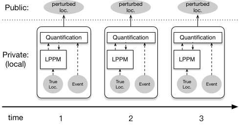
The major components are Quantification and a given LPPM. Their interactions are described as follows. First, the LPPM generates a perturbed location from the true location (Line 2 in Algorithm 1) and pass it to the Quantification component. By Theorem IV.1, the Quantification component (Line 3) checks whether this perturbed location satisfies the ratio in Equation (1) (i.e., $\epsilon$-spatiotemporal event privacy), under a sequence of previous observations and user-specified spatiotemporal events. If not, we need to calibrate the emission matrix to ensure that it satisfies $\epsilon$-spatiotemporal event privacy. The strategy of emission matrix calibration is LPPM-dependent. In the next section, we demonstrate case studies of Geo-Indistinguishability[8] and $\delta$-location set privacy[11], which are the state-of-the-art location privacy metrics.

According to the quantification in Section III, we can calculate $\frac{\Pr(o_{1},o_{2},\cdots,o_{T}|\textsc{Event})}{\Pr(o_{1},o_{2},\cdots,o_{T}|\lnot\textsc{Event})}$ given $o_{1},o_{2},\cdots,o_{T}$ and a given initial probability ${\boldsymbol{\pi}}$. In this section, we show how to make sure the ratio is bounded given arbitrary initial probability.

Our idea to is taking ${\boldsymbol{\pi}}$ as a variable and solving the maximization problem of $\frac{\Pr(o_{1},o_{2},\cdots,o_{T}|\textsc{Event})}{\Pr(o_{1},o_{2},\cdots,o_{T}|\lnot\textsc{Event})}-e^{\epsilon}$. We want to make sure the maximum value is always less than or equal to $0$, i.e., the user enjoys plausible deniability for her specified spatiotemporal event.

The following theorem shows the conditions related to ${\boldsymbol{\pi}}$ that satisfies $\epsilon$-spatiotemporal event privacy. We will formulate it as an optimization problem.

In this section, we instantiate PriSTE framework using $\alpha$-Planar Laplace mechanism ($\alpha$-PLM) which is designed for Geo-indistinguishability[8]. We first show the computation details for quantifying $\epsilon$-spatiotemporal event privacy by Theorem IV.1, and then design a greedy strategy for approximately achieving $\epsilon$-spatiotemporal event privacy.

Algorithm Design. To implement the quantification component, we need to (1) compute the internal parameters a, b and c shown in Theorem IV.1, and (2) design a strategy to calibrate the emission matrix.

For the calibration strategy for Planar Laplace Mechanism (PLM) with a specified privacy budget $\alpha$ (which solely determines the shape of the output distribution), we exponentially decay its privacy budget because a smaller privacy budget implies stronger protection for location privacy and less information disclosure. In our algorithm, decay rate $\frac{1}{2}$ for the privacy budget in line 11 of Algorithm 2 is a tunable parameter that provides a trade-off between efficiency and utility of the released locations. Setting a small value allows the algorithm converge faster, but at the cost of over-perturbing the location at each timestamp. In contrast, using a large value is less efficient but allows better utility to be achieved.

A natural question is whether we can always find an $\alpha$ to release a perturbed location that satisfies Equation (1). The answer is affirmative because $\alpha$ converges exponentially to $0$. When $\alpha=0$, it releases no useful information about the true location, i.e., uniformly returning a random location without using user’s true position. It is easy to verify that the Equations (23) and (24) are always true in this situation.

Algorithm 2 shows the computation process. To boost the efficiency of our algorithm, we use intermediate matrices A and B to facilitate the computation of b and c. At time $1$, we initialize the variables as line $\ref{alg-line-t1-start}\sim\ref{alg-line-t1-end}$. At any time before and inside the Event, we compute the variables as line $\ref{alg-line-in-start}\sim\ref{alg-line-in-end}$. At any timestamps after the Event, the variables are derived as line $\ref{alg-line-out-start}\sim\ref{alg-line-out-end}$. Then we use quadratic programming methods to check Eq.(23) and (24) to decide whether to release the $o_{t}$ or not. If not, we generate a new $o_{t}$ with only half $\alpha$, and repeat the above process again. Finally, we update the matrices A and B as line $\ref{alg-line-AB-start}\sim\ref{alg-line-AB-end}$. If $t=end$, in line 11, the product $\prod_{i=t}^{end-1}\textbf{M}_{i}$ will be the identity matrix. In line 23, $\textbf{M}_{0}$ is the identity matrix when $t=1$. We note that for multiple Events, Algorithm 2 can be executed multiple times for each Event.

To evaluate the effectiveness of PriSTE under different location privacy protection mechanisms, we also instantiate it using another privacy metric $\delta$-location set privacy[11][19], which is proposed for obtaining better utility by taking advantage of temporal correlation between consecutive locations in user’s trajectory. The key idea is that hiding the true location in any impossible locations (e.g., whose probabilities are close to 0) is a lost cause because the adversary already knows the user cannot be there. In other words, it restricts the output domain of the emission matrix to $\delta$-location set, which is a set containing minimum number of locations that have prior probability sum no less than $1-\delta$. A larger $\delta$ indicates weaker privacy guarantee.

The privacy metrics of $\alpha$-geo-indistinguishability and $\delta$-location set privacy are orthogonal because the former requires a specific “shape” of emission distribution and the latter restricts output domain of the emission distribution. In [11], Xiao and Xiong proposed a framework to achieve $\delta$-location set privacy using a given LPPM. For ease of comparison, we use $\alpha$-PLM as the underlying LPPM for $\delta$-location set privacy.

In Line 2, when $t=1$, we have $\mathbf{p}_{0}^{+}=\pi$. In Line 8, according to [11], the posterior probability can be calculated by Equation (30) where $\mathbf{p}_{t}^{+}[j]$ and $\mathbf{p}_{t}^{-}[i]$ are the $i$th elements in the corresponding probability vectors.

Hence, we need the initial probability $\pi$ in order to calculate $\delta$-location set. In experiments, we set $\pi$ to a uniform distribution for the evaluation of $\delta$-location set privacy. We note that PriSTE is agnostic to such initial probability since it guarantees spatiotemporal event privacy against adversaries with arbitrary knowledge about the initial probability.

We generated a synthetic trajectory and its transition probability matrix as follows. First, a map with $20*20$ cells is generated. Then, the transition probability from one cell to another is drawn from the two-dimensional Gaussian distribution with scale parameter $\sigma$ based on the distance between the cells. Here, a smaller $\sigma$ indicates that the user moves to the adjacent cells with a higher probability, i.e., the transition matrix has a more significant pattern. Finally, we produced trajectories with $50$ timestamps using such transition matrix to simulate movement of a user.

References

- [1] Y. Cao, Y. Xiao, L. Xiong, and L. Bai, “PriSTE: from location privacy to spatiotemporal event privacy,” in 2019 IEEE 35th International Conference on Data Engineering (ICDE), 2019, pp. 1606–1609.
- [2] P. Golle and K. Partridge, “On the anonymity of Home/Work location pairs,” in Lecture Notes in Computer Science, 2009, pp. 390–397.
- [3] R. Recabarren and B. Carbunar, “What does the crowd say about you? evaluating aggregation-based location privacy,” in WPES, vol. 2017, 2017, pp. 156–176.
- [4] G. Argyros, T. Petsios, S. Sivakorn, A. D. Keromytis, and J. Polakis, “Evaluating the privacy guarantees of location proximity services,” ACM Trans. Priv. Secur., vol. 19, no. 4, pp. 12:1–12:31, 2017.
- [5] K. Chatzikokolakis, E. ElSalamouny, C. Palamidessi, and P. Anna, “Methods for location privacy: A comparative overview,” Foundations and Trends® in Privacy and Security, vol. 1, no. 4, pp. 199–257, 2017.
- [6] B. Liu, W. Zhou, T. Zhu, L. Gao, and Y. Xiang, “Location privacy and its applications,” IEEE Access, pp. 17 606–17 624, 2018.
- [7] V. Primault, A. Boutet, S. B. Mokhtar, and L. Brunie, “The long road to computational location privacy: A survey,” IEEE Communications Surveys Tutorials, pp. 1–1, 2018.
- [8] M. E. Andrés, N. E. Bordenabe, K. Chatzikokolakis, and C. Palamidessi, “Geo-indistinguishability: differential privacy for location-based systems,” in CCS, 2013, pp. 901–914.
- [9] C. Dwork, “Differential privacy: A survey of results,” in TAMC, 2008, pp. 1–19.
- [10] K. Chatzikokolakis, C. Palamidessi, and M. Stronati, “A predictive differentially-private mechanism for mobility traces,” in Lecture Notes in Computer Science, 2014, no. 8555, pp. 21–41.
- [11] Y. Xiao and L. Xiong, “Protecting locations with differential privacy under temporal correlations,” in CCS, 2015, pp. 1298–1309.
- [12] G. Theodorakopoulos, R. Shokri, C. Troncoso, J.-P. Hubaux, and J.-Y. Le Boudec, “Prolonging the hide-and-seek game: Optimal trajectory privacy for location-based services,” in WPES, 2014, pp. 73–82.
- [13] Y. De Mulder, G. Danezis, L. Batina, and B. Preneel, “Identification via location-profiling in GSM networks,” in WPES, 2008, pp. 23–32.
- [14] M. Asada, M. Yoshikawa, and Y. Cao, ““When and where do you want to hide?” – recommendation of location privacy preferences with local differential privacy,” in Lecture Notes in Computer Science, S. N. Foley, Ed., 2019, pp. 164–176.
- [15] B. Schuster‐Böckler and A. Bateman, “An introduction to hidden markov models,” Current Protocols in Bioinformatics, vol. 18, no. 1, pp. A.3A.1–A.3A.9, 2007.
- [16] Ibm cplex optimizer. [Online]. Available: https://www.ibm.com/analytics/data-science/prescriptive-analytics/cplex-optimizer
- [17] P. M. Pardalos and S. A. Vavasis, “Quadratic programming with one negative eigenvalue is NP-hard,” Journal of Global Optimization, vol. 1, no. 1, pp. 15–22, 1991.
- [18] C. Dwork, M. Naor, T. Pitassi, G. N. Rothblum, and S. Yekhanin, “Pan-private streaming algorithms.” in ICS, 2010, pp. 66–80.
- [19] Y. Xiao, L. Xiong, S. Zhang, and Y. Cao, “LocLok: location cloaking with differential privacy via hidden markov model,” VLDB, vol. 10, no. 12, pp. 1901–1904, 2017.
- [20] Y. Zheng, X. Xie, and W.-Y. Ma, “GeoLife: a collaborative social networking service among user, location and trajectory,” IEEE Data Eng. Bull., vol. 33, no. 2, pp. 32–39, 2010.
- [21] G. Ghinita, M. L. Damiani, C. Silvestri, and E. Bertino, “Preventing velocity-based linkage attacks in location-aware applications,” in SIGSPATIAL, 2009, pp. 246–255.
- [22] C. A. Ardagna, M. Cremonini, S. D. C. d. Vimercati, and P. Samarati, “An obfuscation-based approach for protecting location privacy,” IEEE TDSC, vol. 8, no. 1, pp. 13–27, 2011.
- [23] R. H. Hwang, Y. L. Hsueh, and H. W. Chung, “A novel time-obfuscated algorithm for trajectory privacy protection,” pp. 126–139, 2014.
- [24] S. Takagi, Y. Cao, Y. Asano, and M. Yoshikawa, “Geo-graph-indistinguishability: Protecting location privacy for LBS over road networks,” in DBSec, 2019, pp. 143–163.
- [25] A. Rodriguez-Carrion, D. Rebollo-Monedero, J. Forné, C. Campo, C. Garcia-Rubio, J. Parra-Arnau, and S. K. Das, “Entropy-based privacy against profiling of user mobility,” Entropy, vol. 17, no. 6, pp. 3913–3946, 2015.
- [26] R. Shokri, G. Theodorakopoulos, J.-Y. Le Boudec, and J.-P. Hubaux, “Quantifying location privacy,” in SP, 2011, pp. 247–262.
- [27] N. E. Bordenabe, K. Chatzikokolakis, and C. Palamidessi, “Optimal geo-indistinguishable mechanisms for location privacy,” in CCS, 2014, pp. 251–262.
- [28] R. Shokri, “Privacy games: Optimal user-centric data obfuscation,” PET, vol. 2015, no. 2, 2015.
- [29] Y. Cao and M. Yoshikawa, “Differentially private real-time data release over infinite trajectory streams,” in 2015 16th IEEE International Conference on Mobile Data Management (MDM), vol. 2, 2015, pp. 68–73.
- [30] ——, “Differentially private real-time data publishing over infinite trajectory streams,” IEICE TRANSACTIONS on Information and Systems, vol. E99-D, no. 1, pp. 163–175, 2016.
- [31] F. Xu, Z. Tu, Y. Li, P. Zhang, X. Fu, and D. Jin, “Trajectory recovery from ash: User privacy is NOT preserved in aggregated mobility data,” in WWW, 2017, pp. 1241–1250.
- [32] Y. Cao, M. Yoshikawa, Y. Xiao, and L. Xiong, “Quantifying differential privacy under temporal correlations,” in ICDE, 2017, pp. 821–832.
- [33] ——, “Quantifying differential privacy in continuous data release under temporal correlations,” IEEE Transactions on Knowledge and Data Engineering, vol. 31, no. 7, pp. 1281–1295, 2019.
- [34] Y. Cao, L. Xiong, M. Yoshikawa, Y. Xiao, and S. Zhang, “ConTPL: controlling temporal privacy leakage in differentially private continuous data release,” Proceedings of the VLDB Endowment, vol. 11, no. 12, pp. 2090–2093, 2018.
- [35] L. Liao, D. Fox, and H. Kautz, “Learning and inferring transportation routines,” in AAAI, 2004, pp. 348–353.
- [36] S. Qiao, C. Tang, H. Jin, T. Long, S. Dai, Y. Ku, and M. Chau, “PutMode: prediction of uncertain trajectories in moving objects databases,” Applied Intelligence, vol. 33, no. 3, pp. 370–386, 2010.
- [37] Z. Li, B. Ding, J. Han, and R. Kays, “Swarm: Mining relaxed temporal moving object clusters,” VLDB, vol. 3, no. 1-2, pp. 723–734, 2010.
Appendix A Proofs
A-A Proof of Lemma III.2
A-B Proof of Lemma III.3
A-C Proof of Theorem IV.1
Appendix B Naive Solutions
B-A Computing Prior Probability of an Event
Considering an event is a set of Boolean expression of (location, time) predicates combined with AND and OR, a naive approach would be to enumerate all possible cases for the event and sum (correspond to OR) the product (correspond to AND) of the probabilities of each location predicate and such an approach would require exponential computation time. Due to space limitation, we omit a detailed algorithm for this naive solution. Instead, we show an example as below.
Example B.1.
In Fig.16, a Pattern event is defined by the shaded regions during timestamp to . Thus , . The regions are , , , . To derive the probability of one trajectory, e.g. the solid lines in Fig.16, it would be . Because there are trajectories for the Pattern event, the prior probability of Pattern, i.e., (Pattern) is the sum of such probabilities.
B-B Computing Join Probability of an Event
Let traj be a trajectory of the Pattern. There will be trajectories of the Pattern. For example, in Figure 16, the solid line is , which means in traj is , , in traj is . Let M be the transition matrix where is the transition probability from state to state . denotes the emission probability of observing , . Thus , , . Let be the joint probability of the observations and the trajectory. Then . Thus we focus on the joint probability .
Setup. Let , . For a given , Algorithm 4 can be used to derive the joint probability of a Pattern. The runtime can be compared with the runtime of Equation (21), which is also the joint probability.
Note that to derive Equation (21), we prefer “vector*matrix” instead of “matrix*matrix” for efficiency. Calculate it from left to right so that no matrix multiplication should be conducted.
Appendix C Examples
C-A An Example of Prior Probability Computation
We use an example to describe the details in computation.
Example C.1 (Prior Probability Computation).
Let us consider the computation of Example III.1. For the Presence event defined at and , the transition matrix at and derived by Equation (III-B1) is the left matrix below; while the transition matrix at and derived by Equation (III-B1) is the right matrix below.
Thus by Lemma III.1, , which is a function of as .