Model-independent reconstruction of gravity from Gaussian Processes
Abstract
We apply Gaussian processes and Hubble function data in cosmology, to reconstruct for the first time the form in a model-independent way. In particular, using datasets coming from cosmic chronometers as well as from the radial BAO method, alongside the latest released local value km/s/Mpc, we reconstruct and its derivatives, resulting eventually in a reconstructed region for , without any assumption. Although the cosmological constant lies in the central part of the reconstructed region, the obtained mean curve follows a quadratic function. Inspired by this we propose a new parametrization, i.e. , with the sole free parameter that quantifies the deviation from CDM cosmology. Additionally, we confront three viable one-parameter models of the literature, which respectively are the power-law, the square-root exponential, and the exponential one, with the reconstructed region, and then we extract significantly improved constraints for their model parameters, comparing to the constraints that arise from usual observational analysis. Finally, we argue that since we are using the direct Hubble measurements and the local value for in our analysis, with the above reconstruction of , the tension can be efficiently alleviated.
Keywords:
cosmological parameters, gaussian process, test of modified gravityI Introduction
Modified gravity is an effective approach to describe the early- and late-time universe acceleration (Capozziello 2011a; Nojiri 2010)), except for an introduction of the inflaton and/or dark energy components (Peebles 2002; Cai 2009; Shafieloo 2019; Li 2019; Martiros 2018). In particular, the interest of study upon modified gravity has been revoked in particular by the recently reported measurements of the tension that has failed to be addressed within the standard CDM cosmology (Wong 2019; Freedman 2019; Vagnozzi 2019). Among various constructions of modified gravity one can find the interesting class that is based on the torsional formulation (for a review see (Cai 2015)). In particular, starting from the simplest torsional gravity, namely Teleparallel Equivalent of General Relativity (TEGR) (Einstein 1928; Hayashi 1979; Pereira 2013; Maluf 2013), one can construct modifications such as the gravity (Cai 2015; Bengochea 2008; Linder 2010; Chen 2010; Myrzakulov 2010; Bamba 2010; Dent 2011; Cai 2011; Capozziello 2011b; Wu 2011; Wei 2011; Amoros 2013; Otalora 2013; Bamba 2013; Li 2013; Ong 2013; Nashed 2014; Darabi 2014; Haro 2014; Hanafy 2014; Guo 2015; Bamba 2016; Malekjani 2016; Farrugia 2016; Qi 2017; Bahamonde 2017; Karpathopoulos 2017; Cai 2018; Li 2018; Krššák 2018; Iosifidis 2018; nunes 2018), the gravity (Kofinas 2014a; Kofinas 2014b), scalar-torsion theories (Geng 2011; Hohmann 2018), etc. Finally, one can proceed going beyond the teleparallel framework, and construct more complicated torsional theories.
One key question for any theory of modified gravity is how to determine a viable choice from the arbitrary functions that have been involved. Some general features may be determined by theoretical arguments such as the theoretical requirements for a ghost-free theory that possesses stable perturbations etc, or the desire for the action to possess Noether symmetries; however, the main tool of constraining the possible forms of modification remains that of observational confrontation. The general recipe is to consider by hand a variety of specific forms inside some general class, apply them in a cosmological framework, predict the dynamical behaviours at both the background and perturbation levels, and then use observational data to constrain the involved parameters or exclude the examined form (a similar procedure can also be followed to confront with local/solar system data). For the case of torsional gravity, the cosmological confrontations have been performed in (Wu 2010; Nesseris 2013; Capozziello 2015; Basilakos 2016; Nunes 2016a; Nunes 2016b; Nunes 2018; Basilakos 2018; Anagnostopoulos 2019), and the solar system tests can be found in (Iorio 2012; Iorio 2015; Farrugia 2016), while the latest limit from galaxy lensing has been presented in (Chen 2019). Hence, in the literature there exist at least three viable scenarios for gravity (Nesseris 2013; Basilakos 2018).
Although the above procedure of observational constraints is very useful to offer crucial information on the possible modification forms, it is even more expecting if the data can reconstruct the involved modification functions in a model-independent way without inserting an initial guess. Such a procedure has been successfully developed in the early-time inflationary cosmology (Lidsey 1995; Copeland 1993; Herrera 2018); however, concerning the late-time cosmology the involved complications allow only for a partial application, such as in the cosmography framework (Bamba 2012; Capozziello 2019) or back-scattering procedure (Capozziello 2017). Interestingly, a useful tool towards the above reconstruction is the analysis of Gaussian processes (GP) (Rasmussen 2005; Holsclaw 2010; Seikel 2013), which allow one to investigate features of the form of the involved unknown functions in a model-independent way, using only the given datasets. Such a procedure has been applied to dark energy models using various datasets in order to reconstruct the evolution of the Hubble function, of the dark energy equation-of-state (EoS) parameters, of the dimensionless comoving luminosity distance, of the dark interaction term, etc. (Martiros 2018; Seikel 2012; Shafieloo 2012; Seikel 2013; Kim 2013; Nair 2013; Yang 2015; Costa 2015; Zhang 2016; Wang 2017; Gomez-Valent 2018; Pinho 2018; Elizalde 2018; Melia 2018; Pinho 2018; Zhang 2018; Yin 2018; Rau 2019; Gomez-Valent 2019).
In this article we develop the GP analysis for the case of cosmology, in order to reconstruct the form of the modification in a model-independent way, namely using as the only input the observational datasets of Hubble function measurements . Such a procedure becomes easy in the case of cosmology, since the latter has the advantage that the torsion scalar is a simple function of , namely , and thus eventually all cosmological equations can be expressed in terms of and its derivative. Hence, reconstructing and its derivative from the Hubble data through the GP analysis, leads to the reconstruction of the form itself, without any assumption.
The plan of the article is as follows. In Section II we provide a brief review of the cosmological equations of gravity. In Section III we describe the basic ingredients of GP and then we apply it for Hubble function observational data reconstructing and its derivative. Then in Section IV we use this reconstruction in order to reconstruct the form of in a model-independent way, and to extract constraint on various models in the literature. Finally, in Section V we summarize our results with a discussion.
II gravity and cosmology
In this section we briefly review gravity and cosmology. In torsional formulation one uses as dynamical variables the vierbeins fields, which form an orthonormal basis at a manifold point. In a coordinate basis they are related to the metric through , with Greek and Latin indices respectively used for the coordinate and tangent space. In the particular class of teleparallel gravity one introduces the Weitzenböck connection (Weitzenböck 1923), and thus the corresponding torsion tensor is
| (1) |
while the corresponding curvature tensor is zero. We mention here that the above formulation is constructed in a specific cosmological gauge where the spin connection components are vanishing, which simplifies the analysis and allows us to impose the specific vierbein choice below. Leaving a non-zero spin connection is also possible, however this would involve more complicated vierbeins (Krššák 2015; Hohmann 2018).
The torsion tensor incorporates all the information of the gravitational field, and the torsion scalar arises from its contraction as
| (2) |
This forms the Lagrangian of teleparallel gravity (similarly to general relativity where the Lagrangian is the Ricci scalar), and since variation in terms of the vierbeins gives the same equations with general relativity, the constructed theory was named teleparallel equivalent of general relativity (TEGR).
One can start from TEGR to proceed the torsional based modifications. The simplest extension is to generalize in the action to be (Cai 2015),
| (3) |
where , is the gravitational constant, and where for completeness we have also included the matter Lagrangian . Variation of the above action results to the field equations
| (4) |
with , , and where denotes the total matter (namely dark and baryonic matter) energy-momentum tensor. Finally, is the super-potential, with the contorsion tensor.
In order to apply gravity at a cosmological framework we impose the spatially flat Friedmann-Lemaître-Robertson-Walker (FLRW) metric
| (5) |
which corresponds to the vierbein form , where is the scale factor. Inserting this choice into the general field equations (II) we result to the Friedmann equations of cosmology, namely
| (6) | ||||
| (7) |
with the Hubble function and where dots denoting derivatives with respect to . Additionally, in the above equations and are respectively the energy density and pressure of the matter fluid. Note that the torsion scalar (2) in FRW geometry becomes
| (8) |
and this expression proves very useful for the purpose of the present work.
As a next step we define an effective dark energy sector with energy density and pressure respectively given by
| (9) | ||||
| (10) |
and therefore its EoS parameter reads as
| (11) |
Hence, the first Friedmann equation (6) effectively acquires the standard form . Finally, the system of cosmological equations closes by considering the matter conservation
| (12) |
which using (6), (7) implies additionally the conservation of the effective dark energy,
| (13) |
III Gaussian Process using data
In this section we first present the general steps of the GP approach, and then we apply it in the case where the inserted data come from Hubble function observations.
III.1 Gaussian Process
The GP is a powerful tool allowing to reconstruct the behavior of a function (and its derivatives) directly from given datasets (Seikel 2012). The basic ingredients of the GP techniques are the covariance function (kernel), and the feature that the parameters describing it can be estimated directly from observational data (Seikel 2012). Hence, one does not need to consider any specific parametrization for the involved unknown function of the model, since it can be reconstructed from observational data directly by using the cosmological equations.
In GP one assumes that the observations of the dataset are sampled from a multi-variance Gaussian distribution. Moreover, the values of the function evaluated at different points are not independent, and the connection between neighbouring points is due to the covariance functions chosen in advance. The Gaussian distribution corresponds to a random variable characterized by a mean value and a covariance. Similar to Gaussian distributions, GPs should be understood as distributions over functions, determined by a mean function and a covariance matrix. Since the covariance function, for a given set of observations, can infer the relation between independent and dependent variables, using the covariance function the GP correlates the function at different points.
There exists a number of possible choices for the covariance function, i.e., for the kernel, e.g. squared exponential, polynomial, spline, etc, used in various applications (Rasmussen 2005). Although there is a discussion on possible effects of the kernel choice on the results (Rasmussen 2005; Seikel 2013) (in a similar way that there is a discussion of the possible effect of the covariance matrix choice on the usual observational fittings (Eifler 2008; Morrison 2013)), one commonly used choice, with good theoretical justification, is the squared exponential function (Rasmussen 2005; Seikel 2013)
| (14) |
where and are parameters known as hyper-parameters. These parameters represent the length scales in the GP. In particular, corresponds to the correlation length along which the successive values are correlated, while to control the variation in relative to the mean of the process we need the parameter . Therefore, the covariance between output variables will be written as a function of the input ones. We mention that the covariance is maximum for variables whose inputs are suitably close. Furthermore, as can be seen from (14), the squared exponential function is infinitely differentiable, which proves to be a useful property in case of reconstructing higher-order derivatives. Additionally, the initial and effective approach adopted in GP to estimate the values of the hyperparameters, is based on the training by maximizing the likelihood, showing that the reconstructed function has the measured values at the data points.
Finally, we mention that the consideration of the squared exponential kernel is the most natural choice amongst various possibilities, given the assumption that the error distribution for the observational data is the Gaussian one (Rasmussen 2005; Seikel 2013). 11 1 Another choice can be the so-called Matern () covariance function (Rasmussen 2005; Seikel 2013) with and the hyper-parameters. However, its application leads to similar results with the squared exponential function (14), namely coincidence within 1 (Elizalde 2018). Indeed, repeating the analysis of the present work using this alternative kernel shows that the difference between the results is within . Therefore, taking into account this fact, in this article we proceed only with the squared exponential kernel choice, namely (14).
III.2 data
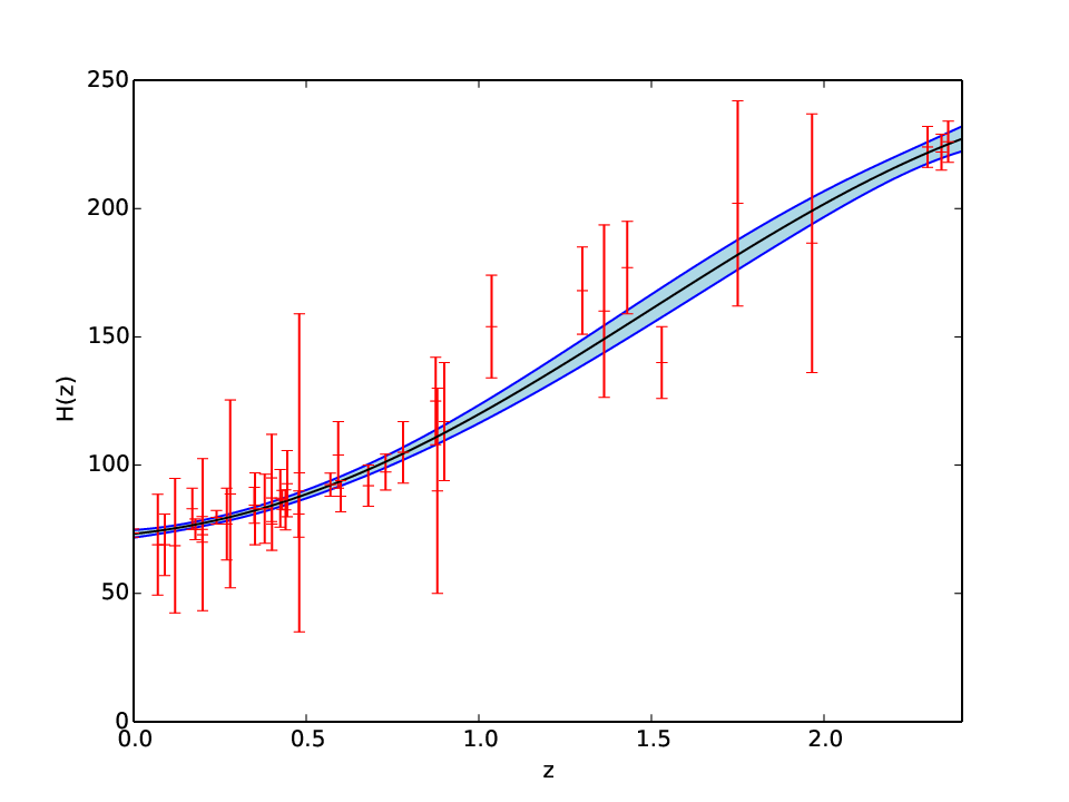
In this work we will use GP techniques with Hubble data (, with the present scale factor). In particular, we use -point samples of arising from the differential evolution of cosmic chronometers, alongside -point samples obtained from the radial BAO method, which allows to extend the data range up to , improving also the behavior at low redshifts. In Table 1 we present the above points as they appear in (Zhang 2016). We note that in principle the use of data points from different datasets should be avoided, however, as it was discussed in (Seikel 2012), the simultaneous use of the above two data sets gives the increased statistics that it is necessary for the correct application of the GP. Finally, concerning the value of the Hubble parameter at present , we use the latest released local value at 2.4% precision, namely km/s/Mpc (Riess 2016). We mention here that since we are using the direct Hubble measurements and the local value for , in our analysis and hence in our reconstruction, the tension is alleviated by construction. 22 2 Accompanied with the as well as tensions, another model-independent approach of alleviation can be achieved by virtue of the effective field theory approach as shown in (Yan 2019).
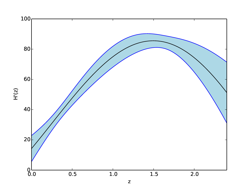
We use the publicly available package GaPP (Gaussian Processes in Python) developed by Seikel et al. (Seikel 2012), and we apply it for the aforementioned data. The result of this elaboration is the successful reconstruction of and (primes denote derivative with respect to the redshift ) in a model-independent way. In Figure 1, the numerically derived mean curves and their 1 errors are presented 33 3 Note that, although we have imposed the value km/s/Mpc, the GP reconstruction itself provides an automatically tuned value around km/s/Mpc at , which remains self consistent.. These reconstructions shall be used to reconstruct the forms in the next section.
IV Reconstructing form from GP
In the previous section we applied the GP in the data, and we resulted in the reconstruction of and its derivatives, in a model-independent way, namely without assuming anything on the underlying gravitational theory or cosmological scenario. In this section we will assume that the universe is governed by gravity, hence we will use the cosmological equations of Section II, and we will use the reconstructed and its derivatives to reconstruct the form of without any other assumption. Up to our knowledge it is for the first time that this is performed, since up to now in the literature a specific ansatz for was always imposed by hand and then the confrontation with the data led to constraining the involved parameters.
The basic feature of gravity that makes the above reconstruction procedure easy is the fact that in FRW geometry for the torsion scalar we have relation (8), namely , i.e. it is a simple function of . Thus, all the involved terms and functions of cosmology can eventually be expressed in terms of and its derivatives, which have been reconstructed through GP in the previous section. Hence, the final step of this analysis is the reconstruction of the form itself.
We start by expressing all cosmological equations of Section II in terms of the redshift . For the time derivative of a function we have , where the prime denotes derivative with respect to , while for we have
| (15) |
The next step in the application of the GP is to replace by
| (16) |
for small , which allows to relate the values of at and . In particular, it is easy to see that from Equation (6) one acquires
| (17) | ||||
where and . Moreover, for the matter sector we adopt the EoS parameter for regular dust, which eventually gives
| (18) |
due to (12). Here and are the Hubble parameter and the dark matter density parameter () at . Inserting these into (17) we finally obtain
| (19) | ||||
Equation (19) allows us to reconstruct , as long as and are known. However, in the previous sections we were able to reconstruct and from the Hubble data. Thus, the reconstruction of is straightforward. Finally, since both and are reconstructed, we can easily reconstruct the form of in a model-independent way.
In Figure 2 we present the reconstructed resulting from our analysis, which is the main result of the present work. Let us now try to extract information on the possible forms of .
The first and clear result is that the form, namely the cosmological constant, lies in the central part of the reconstructed region, and in particular with the value (the dotted line of Figure 2) which is exactly the cosmological constant one ( ) as expected.
Nevertheless, from the reconstructed region of Figure 2 we can obtain additional information, namely what is the form of the mean reconstructed curve (the black curve of Figure 2).

In particular, as we can see the mean curve is not a constant, but its best fit (with accuracy ) follows a quadratic function of the form , with (i.e. is not a free parameter) and the two parameters , in units of km/s/Mpc. Since the linear term can be removed from and be absorbed by the standard linear term that exists already in (3), the above form remains with one free parameter namely , as it is the case in all viable models (that is why we did not allow for a second free parameter, namely , although in this case the fitting is significantly improved at ). Hence, in summary, the mean curve of the reconstructed procedure follows the quadratic form
| (20) |
with the sole free parameter. Note that, if we use a dimensionless free parameter then we may re-write (20) as , with , and hence with the dimensionless parameter .
However, besides the mean curve of the reconstruction, in principle any curve inside the shaded region of Figure 2 is allowed to be the true form. Hence, let us confront three viable one-parameter models of the literature (Nesseris 2013; Basilakos 2018), with our reconstructed region. In particular, they are the power-law (CDM) model
| (21) |
with , the square-root exponential (CDM) model
| (22) |
with and , and the exponential (CDM) model
| (23) |
with . These models coincide with CDM for (model (21)), and for (models (22) and (23)).


As shown in Figure 3, if we expect the above forms to lie inside the reconstructed region we obtain the following constraints on their sole parameter: for the power-law (CDM) model, for the square-root exponential (CDM) model, and for the exponential (CDM) model. Interestingly enough, these constraints are improved comparing to the constraints coming from usual observational analysis using Supernovae type Ia, quasi-stellar objects, Cosmic Microwave Background shift parameter, direct Hubble constant measurements with cosmic chronometers, and redshift space distortion () measurements, which give for the power law, for the square-root exponential, and for the exponential models (Basilakos 2018; Anagnostopoulos 2019). Note the significant improvement by two orders of magnitude in the case of the power-law model. This is one of the main results of the present work, and shows the capabilities of the reconstruction procedure using GP.
Finally, concerning the quadratic form of in Equation (20), we deduce that in order to lie inside the reconstructed region its free parameter should be constrained as (in units of (km/s/Mpc)-4). Equivalently, using the dimensional parameter discussed above, we derive that . Hence, in the present work we propose the new parametrization (20), since it can also be efficient in describing the reconstructed region that was obtained from the Hubble data through the GP analysis. The efficiency of the quadratic form was actually expected, since at late times where and thus are small, every function can be expanded in -series (Iorio 2012; Nashed 2015; Farrugia 2016; Bahamonde 2019; Chen 2019).
V Conclusions
In this work we have applied the GP analysis and Hubble function data in cosmology, to reconstruct for the first time the form in a model-independent way. In particular, up to now in the literature of gravity, as well as in the majority of gravitational modifications, physicists were assuming specific ansatz for the involved unknown function, and were using observational data in order to constrain the model parameters. However, the use of the GP analysis allows to investigate features of the form of the involved unknown functions in a model-independent way without any assumption, using only the given observational datasets.
We applied the GP analysis for Hubble function measurements, namely for datasets coming from cosmic chronometers as well as from the radial BAO method, alongside the latest released local value km/s/Mpc at 2.4% precision. Application of the procedure led to the reconstruction of and its derivative without any assumption. On the other hand, cosmology has the advantage that the torsion scalar is a simple function of , namely , and thus eventually all cosmological equations can be expressed in terms of ,. Hence, having reconstructed and allowed us to additionally reconstruct the form itself, without any assumption. Up to our knowledge this is the first time where a general and model-independent reconstruction for the gravity is obtained. Additionally, we mention that since we are using the direct Hubble measurements and the local value for , in our analysis and hence in our reconstruction, the tension can be alleviated by construction.
A first result of our analysis is that the cosmological constant lies in the central part of the reconstructed region, as expected. However, the mean curve of the reconstructed region is not a constant, but its best fit follows a quadratic function. Hence, inspired by this, in this work we proposed a new one-parameter parametrization, namely , with and the sole free parameter that quantifies the deviation from CDM cosmology. Moreover, fitting this form into the reconstructed region we extracted the constraints on the free parameter as (km/s/Mpc)-4.
Additionally, we have confronted three viable one-parameter models of with the reconstructed region, which are the power-law, square-root exponential, and exponential one, respectively. As shown in the main text, we obtained improved constraints for their free parameters, comparing to the bounds that arise from traditional observational analyses, and especially for the case of the power-law model the improvement was more than two-orders of magnitude.
In summary, using GPs and Hubble data we obtained a model-independent reconstruction for the form, and fitting its mean curve we proposed a new one-parameter parametrization, namely the quadratic one. Finally, confronting three viable models of the literature with our reconstructed region, we extracted improved constraints on their parameters. These features reveal the capabilities of the reconstruction procedure using GPs. Hence, it would be interesting to apply them in other theories of modified gravity too.
Acknowledgments
We thank Canmin Deng, Rafael Nunes, Xin Ren, Yuting Wang and Gongbo Zhao for valuable comments. We also thank the anonymous referee for constructive comments. YFC is supported in part by the National Youth Thousand Talents Program of China, by NSFC (Nos. 11722327, 11653002, 11961131007, 11421303), by CAST (2016QNRC001), and by the Fundamental Research Funds for Central Universities. MK is supported in part by a CAS President’s International Fellowship Initiative Grant (No. 2018PM0054) and by NSFC (No. 11847226). ENS is supported partly by USTC fellowship for international visiting professors. This article is partially based upon work from COST Action “Cosmology and Astrophysics Network for Theoretical Advances and Training Actions”, supported by COST (European Cooperation in Science and Technology). All numerics were operated on the computer clusters Linda & Judy in the particle cosmology group at USTC.
References
- Capozziello (2011a) S. Capozziello and M. De Laurentis, Phys. Rept. 509, 167 (2011) [arXiv:1108.6266 [gr-qc]].
- Nojiri (2010) S. Nojiri and S. D. Odintsov, Phys. Rept. 505, 59 (2011) [arXiv:1011.0544 [gr-qc]].
- Peebles (2002) P. J. E. Peebles and B. Ratra, Rev. Mod. Phys. 75, 559 (2003) [astro-ph/0207347].
- Cai (2009) Y. F. Cai, E. N. Saridakis, M. R. Setare and J. Q. Xia, Phys. Rept. 493, 1 (2010) [arXiv:0909.2776 [hep-th]].
- Shafieloo (2019) X. Li, A. Shafieloo, arXiv:1906.08275 [astro-ph.CO].
- Li (2019) X. L. Li, A. Shafieloo, V. Sahni, A. A. Starobinsky, arXiv:1904.03790 [astro-ph.CO].
- Martiros (2018) E. Elizalde, M. Khurshudyan, S. Nojiri, Int. J. Mod. Phys. D 28, no.01, 1950019 (2018) [arXiv:1809.01961 [gr-qc]].
- Wong (2019) K. C. Wong et al., arXiv:1907.04869 [astro-ph.CO].
- Freedman (2019) W. L. Freedman et al., arXiv:1907.05922 [astro-ph.CO].
- Vagnozzi (2019) S. Vagnozzi, arXiv:1907.07569 [astro-ph.CO].
- Cai (2015) Y. F. Cai, S. Capozziello, M. De Laurentis and E. N. Saridakis, Rept. Prog. Phys. 79, no. 10, 106901 (2016) [arXiv:1511.07586 [gr-qc]].
- Einstein (1928) A. Einstein 1928, Sitz. Preuss. Akad. Wiss. p. 217; ibid p. 224; A. Unzicker and T. Case, physics/0503046.
- Hayashi (1979) K. Hayashi and T. Shirafuji, Phys. Rev. D 19, 3524 (1979); Addendum-ibid. 24, 3312 (1982).
- Pereira (2013) R. Aldrovandi, J.G. Pereira, Teleparallel Gravity: An Introduction, Springer, Dordrecht, 2013.
- Maluf (2013) J. W. Maluf, Annalen Phys. 525, 339 (2013) [arXiv:1303.3897 [gr-qc]].
- Bengochea (2008) G. R. Bengochea and R. Ferraro, Phys. Rev. D 79, 124019 (2009) [arXiv:0812.1205 [astro-ph]].
- Linder (2010) E. V. Linder, Phys. Rev. D 81, 127301 (2010) Erratum: [Phys. Rev. D 82, 109902 (2010)] [arXiv:1005.3039 [astro-ph.CO]].
- Chen (2010) S. H. Chen, J. B. Dent, S. Dutta and E. N. Saridakis, Phys. Rev. D 83, 023508 (2011) [arXiv:1008.1250 [astro-ph.CO]].
- Myrzakulov (2010) R. Myrzakulov, Gen. Rel. Grav. 44, 3059 (2012) [arXiv:1008.4486 [physics.gen-ph]].
- Bamba (2010) K. Bamba, C. Q. Geng, C. C. Lee and L. W. Luo, JCAP 1101, 021 (2011) [arXiv:1011.0508 [astro-ph.CO]].
- Dent (2011) J. B. Dent, S. Dutta and E. N. Saridakis, JCAP 1101, 009 (2011) [arXiv:1010.2215 [astro-ph.CO]].
- Cai (2011) Y. F. Cai, S. H. Chen, J. B. Dent, S. Dutta and E. N. Saridakis, Class. Quant. Grav. 28, 215011 (2011) [arXiv:1104.4349 [astro-ph.CO]].
- Capozziello (2011b) S. Capozziello, V. F. Cardone, H. Farajollahi and A. Ravanpak, Phys. Rev. D 84, 043527 (2011) [arXiv:1108.2789 [astro-ph.CO]].
- Wu (2011) Y. P. Wu and C. Q. Geng, Phys. Rev. D 86, 104058 (2012) [arXiv:1110.3099 [gr-qc]].
- Wei (2011) H. Wei, X. J. Guo and L. F. Wang, Phys. Lett. B 707, 298 (2012) [arXiv:1112.2270 [gr-qc]].
- Amoros (2013) J. Amoros, J. de Haro and S. D. Odintsov, Phys. Rev. D 87, 104037 (2013) [arXiv:1305.2344 [gr-qc]].
- Otalora (2013) G. Otalora, Phys. Rev. D 88, 063505 (2013) [arXiv:1305.5896 [gr-qc]].
- Bamba (2013) K. Bamba, S. D. Odintsov and D. Saez-Gomez, Phys. Rev. D 88, 084042 (2013) [arXiv:1308.5789 [gr-qc]].
- Li (2013) J. T. Li, C. C. Lee and C. Q. Geng, Eur. Phys. J. C 73, no. 2, 2315 (2013) [arXiv:1302.2688 [gr-qc]].
- Ong (2013) Y. C. Ong, K. Izumi, J. M. Nester and P. Chen, Phys. Rev. D 88, 024019 (2013) [arXiv:1303.0993 [gr-qc]].
- Nashed (2014) G. G. L. Nashed and W. El Hanafy, Eur. Phys. J. C 74, 3099 (2014) [arXiv:1403.0913 [gr-qc]].
- Darabi (2014) F. Darabi, M. Mousavi and K. Atazadeh, Phys. Rev. D 91, 084023 (2015) [arXiv:1501.00103 [gr-qc]].
- Haro (2014) J. Haro and J. Amoros, JCAP 1412, no. 12, 031 (2014) [arXiv:1406.0369 [gr-qc]].
- Hanafy (2014) W. El Hanafy and G. G. L. Nashed, Eur. Phys. J. C 75, 279 (2015) [arXiv:1409.7199 [hep-th]].
- Guo (2015) W. D. Guo, Q. M. Fu, Y. P. Zhang and Y. X. Liu, Phys. Rev. D 93, no. 4, 044002 (2016) [arXiv:1511.07143 [hep-th]].
- Bamba (2016) K. Bamba, G. G. L. Nashed, W. El Hanafy and S. K. Ibraheem, Phys. Rev. D 94, no. 8, 083513 (2016) [arXiv:1604.07604 [gr-qc]].
- Malekjani (2016) M. Malekjani, N. Haidari and S. Basilakos, Mon. Not. Roy. Astron. Soc. 466, no. 3, 3488 (2017) [arXiv:1609.01964 [gr-qc]].
- Farrugia (2016) G. Farrugia and J. L. Said, Phys. Rev. D 94, no. 12, 124054 (2016) [arXiv:1701.00134 [gr-qc]].
- Bahamonde (2017) S. Bahamonde, C. G. Böhmer and M. Krššák, Phys. Lett. B 775, 37 (2017) [arXiv:1706.04920 [gr-qc]].
- Qi (2017) J. Z. Qi, S. Cao, M. Biesiada, X. Zheng and H. Zhu, Eur. Phys. J. C 77, no. 8, 502 (2017) [arXiv:1708.08603 [astro-ph.CO]].
- Karpathopoulos (2017) L. Karpathopoulos, S. Basilakos, G. Leon, A. Paliathanasis and M. Tsamparlis, Gen. Rel. Grav. 50, 79 (2018) [arXiv:1709.02197 [gr-qc]].
- Cai (2018) Y. F. Cai, C. Li, E. N. Saridakis and L. Xue, Phys. Rev. D 97, no. 10, 103513 (2018) [arXiv:1801.05827 [gr-qc]].
- Li (2018) C. Li, Y. Cai, Y. F. Cai and E. N. Saridakis, JCAP 1810, no. 10, 001 (2018) [arXiv:1803.09818 [gr-qc]].
- Krššák (2018) M. Krššák, R. J. Van Den Hoogen, J. G. Pereira, C. G. Boehmer and A. A. Coley, arXiv:1810.12932 [gr-qc].
- Iosifidis (2018) D. Iosifidis and T. Koivisto, arXiv:1810.12276 [gr-qc].
- nunes (2018) R. C.Nunes, JCAP 05, 052 (2018) [arXiv:1802.02281 [gr-qc]].
- Kofinas (2014a) G. Kofinas and E. N. Saridakis, Phys. Rev. D 90, 084044 (2014) [arXiv:1404.2249 [gr-qc]].
- Kofinas (2014b) G. Kofinas and E. N. Saridakis, Phys. Rev. D 90, 084045 (2014) [arXiv:1408.0107 [gr-qc]].
- Geng (2011) C. Q. Geng, C. C. Lee, E. N. Saridakis and Y. P. Wu, Phys. Lett. B 704, 384 (2011) [arXiv:1109.1092 [hep-th]].
- Hohmann (2018) M. Hohmann, L. Jarv and U. Ualikhanova, Phys. Rev. D 97, no. 10, 104011 (2018) [arXiv:1801.05786 [gr-qc]].
- Wu (2010) P. Wu and H. W. Yu, Phys. Lett. B 693, 415 (2010) [arXiv:1006.0674 [gr-qc]].
- Nesseris (2013) S. Nesseris, S. Basilakos, E. N. Saridakis and L. Perivolaropoulos, Phys. Rev. D 88, 103010 (2013) [arXiv:1308.6142 [astro-ph.CO]].
- Capozziello (2015) S. Capozziello, O. Luongo and E. N. Saridakis, Phys. Rev. D 91, no. 12, 124037 (2015) [arXiv:1503.02832 [gr-qc]].
- Basilakos (2016) S. Basilakos, Phys. Rev. D 93, no. 8, 083007 (2016) [arXiv:1604.00264 [gr-qc]].
- Nunes (2016a) R. C. Nunes, S. Pan and E. N. Saridakis, JCAP 1608, no. 08, 011 (2016) [arXiv:1606.04359 [gr-qc]].
- Nunes (2016b) R. C. Nunes, A. Bonilla, S. Pan and E. N. Saridakis, Eur. Phys. J. C 77, no. 4, 230 (2017) [arXiv:1608.01960 [gr-qc]].
- Nunes (2018) R. C. Nunes, JCAP 1805, no. 05, 052 (2018) [arXiv:1802.02281 [gr-qc]].
- Basilakos (2018) S. Basilakos, S. Nesseris, F. K. Anagnostopoulos and E. N. Saridakis, JCAP 1808, no. 08, 008 (2018) [arXiv:1803.09278 [astro-ph.CO]].
- Anagnostopoulos (2019) F. K. Anagnostopoulos, S. Basilakos and E. N. Saridakis, arXiv:1907.07533 [astro-ph.CO].
- Iorio (2012) L. Iorio and E. N. Saridakis, Mon. Not. Roy. Astron. Soc. 427, 1555 (2012) [arXiv:1203.5781 [gr-qc]].
- Iorio (2015) L. Iorio, N. Radicella and M. L. Ruggiero, JCAP 1508, no. 08, 021 (2015) [arXiv:1505.06996 [gr-qc]].
- Farrugia (2016) G. Farrugia, J. L. Said and M. L. Ruggiero, Phys. Rev. D 93, no. 10, 104034 (2016) [arXiv:1605.07614 [gr-qc]].
- Bahamonde (2019) S. Bahamonde, K. Flathmann and C. Pfeifer, Phys. Rev. D 100, no. 8, 084064 (2019) doi:10.1103/PhysRevD.100.084064 [arXiv:1907.10858 [gr-qc]].
- Chen (2019) Z. Chen, W. Luo, Y. F. Cai and E. N. Saridakis, arXiv:1907.12225 [astro-ph.CO].
- Lidsey (1995) J. E. Lidsey, A. R. Liddle, E. W. Kolb, E. J. Copeland, T. Barreiro and M. Abney, Rev. Mod. Phys. 69, 373 (1997) [astro-ph/9508078].
- Copeland (1993) E. J. Copeland, E. W. Kolb, A. R. Liddle and J. E. Lidsey, Phys. Rev. D 48, 2529 (1993) [hep-ph/9303288].
- Herrera (2018) R. Herrera, Phys. Rev. D 98, no. 2, 023542 (2018) [arXiv:1805.01007 [gr-qc]].
- Bamba (2012) K. Bamba, S. Capozziello, S. Nojiri and S. D. Odintsov, Astrophys. Space Sci. 342, 155 (2012) [arXiv:1205.3421 [gr-qc]].
- Capozziello (2019) S. Capozziello, R. D’Agostino and O. Luongo, arXiv:1904.01427 [gr-qc].
- Capozziello (2017) S. Capozziello, R. D’Agostino and O. Luongo, Gen. Rel. Grav. 49, no. 11, 141 (2017) [arXiv:1706.02962 [gr-qc]].
- Rasmussen (2005) C. E. Rasmussen and C. K. I. Williams, Gaussian Processes for Machine Learning, The MIT Press, (2005).
- Holsclaw (2010) T. Holsclaw, U. Alam, B. Sanso, H. Lee, K. Heitmann, S. Habib and D. Higdon, Phys. Rev. Lett. 105, 241302 (2010) [arXiv:1011.3079 [astro-ph.CO]].
- Seikel (2013) M. Seikel and C. Clarkson, arXiv:1311.6678 [astro-ph.CO].
- Seikel (2012) M. Seikel, C. Clarkson and M. Smith, JCAP 1206, 036 (2012) [arXiv:1204.2832 [astro-ph.CO]].
- Shafieloo (2012) A. Shafieloo, A. G. Kim and E. V. Linder, Phys. Rev. D 85, 123530 (2012) [arXiv:1204.2272 [astro-ph.CO]].
- Kim (2013) A. G. Kim et al., Astrophys. J. 766, 84 (2013) [arXiv:1302.2925 [astro-ph.CO]].
- Nair (2013) R. Nair, S. Jhingan and D. Jain, JCAP 1401, 005 (2014) [arXiv:1306.0606 [astro-ph.CO]].
- Yang (2015) T. Yang, Z. K. Guo and R. G. Cai, Phys. Rev. D 91, no. 12, 123533 (2015) [arXiv:1505.04443 [astro-ph.CO]].
- Costa (2015) S. Santos-da-Costa, V. C. Busti and R. F. L. Holanda, JCAP 1510, no. 10, 061 (2015) [arXiv:1506.00145 [astro-ph.CO]].
- Zhang (2016) M. J. Zhang and J. Q. Xia, JCAP 1612, no. 12, 005 (2016) [arXiv:1606.04398 [astro-ph.CO]].
- Wang (2017) D. Wang and X. H. Meng, Phys. Rev. D 95, no. 2, 023508 (2017) [arXiv:1708.07750 [astro-ph.CO]].
- Gomez-Valent (2018) A. Gomez-Valent and L. Amendola, JCAP 1804, no. 04, 051 (2018) [arXiv:1802.01505 [astro-ph.CO]].
- Melia (2018) F. Melia and M. K. Yennapureddy, JCAP 1802, no. 02, 034 (2018) [arXiv:1802.02255 [astro-ph.CO]].
- Pinho (2018) A. M. Pinho, S. Casas and L. Amendola, JCAP 1811, no. 11, 027 (2018) [arXiv:1805.00027 [astro-ph.CO]].
- Zhang (2018) M. J. Zhang and H. Li, Eur. Phys. J. C 78, no. 6, 460 (2018) [arXiv:1806.02981 [astro-ph.CO]].
- Yin (2018) Z. Y. Yin and H. Wei, Sci. China Phys. Mech. Astron. 62, no. 9, 999811 (2019) [arXiv:1808.00377 [astro-ph.CO]].
- Elizalde (2018) E. Elizalde and M. Khurshudyan, Phys. Rev. D 99, no. 10, 103533 (2019) [arXiv:1811.03861 [astro-ph.CO]].
- Pinho (2018) A. M. Pinho, S. Casas, L. Amendola, JCAP 1811, 027 (2018) [arXiv:1805.00027 [astro-ph.CO]].
- Rau (2019) M. M. Rau, S. Wilson and R. Mandelbaum, arXiv:1904.09988 [astro-ph.CO].
- Gomez-Valent (2019) A. Gomez-Valent and L. Amendola, arXiv:1905.04052 [astro-ph.CO].
- Weitzenböck (1923) Weitzenböck R., Invarianten Theorie, Nordhoff, Groningen (1923).
- Krššák (2015) M. Krššák and E. N. Saridakis, Class. Quant. Grav. 33, no. 11, 115009 (2016) [arXiv:1510.08432 [gr-qc]].
- Eifler (2008) T. Eifler, P. Schneider and J. Hartlap, Astron. Astrophys. 502, 721 (2009) [arXiv:0810.4254 [astro-ph]].
- Morrison (2013) C. B. Morrison and M. D. Schneider, JCAP 1311, 009 (2013) [arXiv:1304.7789 [astro-ph.CO]].
- Aghanim (2018) N. Aghanim et al. [Planck Collaboration], arXiv:1807.06209 [astro-ph.CO].
- Riess (2016) A. G. Riess et al., Astrophys. J. 826, no. 1, 56 (2016) [arXiv:1604.01424 [astro-ph.CO]].
- Yan (2019) S. F. Yan, P. Zhang, J. W. Chen, X. Z. Zhang, Y. F. Cai and E. N. Saridakis, arXiv:1909.06388 [astro-ph.CO].
- Nashed (2015) G. L. Nashed Gen. Rel. Grav. 47, no. 7, 75 (2015) [arXiv:1506.08695 [gr-qc]].