Transport Monte Carlo:
High-Accuracy Posterior Approximation
via Random Transport

Leo L. Duan Thanks: Department of Statistics, University of Florida, Gainesville, FL, email: li.duan@ufl.edu

Abstract: In Bayesian applications, there is a huge interest in rapid and accurate estimation of the posterior distribution, particularly for high dimensional or hierarchical models. In this article, we propose to use optimization to solve for a joint distribution (random transport plan) between two random variables, $\theta$ from the posterior distribution and $\beta$ from the simple multivariate uniform. Specifically, we obtain an approximate estimate of the conditional distribution $\Pi(\beta\mid\theta)$ as an infinite mixture of simple location-scale changes; applying the Bayes’ theorem, $\Pi(\theta\mid\beta)$ can be sampled as one of the reversed transforms from the uniform, with the weight proportional to the posterior density/mass function. This produces independent random samples with high approximation accuracy, as well as nice theoretic guarantees. Our method shows compelling advantages in performance and accuracy, compared to the state-of-the-art Markov chain Monte Carlo and approximations such as variational Bayes and normalizing flow. We illustrate this approach via several challenging applications, such as sampling from multi-modal distribution, estimating sparse signals in high dimension, and soft-thresholding of a graph with a prior on the degrees.
KEYWORDS: Infinite Mixture, Monge and Kantorovich Transports, Non-invertible Transport, Simple Function Approximation.

1 Introduction

The Bayesian framework is routinely used to impose model regularization and obtain uncertainty quantification. As the posterior distribution often does not have a closed-form, it is common to rely on the Monte Carlo estimation. The Markov chain Monte Carlo (MCMC) has been the most popular method due to the ability to alternatively update one part of the parameter each time; often, each conditional update is easy to carry out, such as having tractable full conditional form. As a side effect, this creates a Markov chain dependency among the collected samples; to reduce this effect, one can filter down the collected Markov chain (often known as “thinning”), by keeping the samples that are a few iterations apart and discarding the ones in between.

A primary challenge is that modern Bayesian applications often face complications such as high dimensionality or hierarchical structure, the above computing strategy can become very inefficient: since each update corresponds to a small local change, the Markov chain will still be highly auto-correlated, even after a sizeable amount of thinning. This is known as the low effective sample size problem, or slow mixing of Markov chains. This issue has been well known for a long time in the community, yet it was formally studied only until recently. See Rajaratnam and Sparks 2015 on the failing of convergence rate guarantee in high dimension, Johndrow et al. 2019 on the case of imbalanced categorical data, Duan et al. 2018 on the need to calibrate the step size for data augmentation, etc. For a recent survey on this issue, see Robert et al. 2018. This issue has motivated a large literature of new Markov chain methods, using different proposing algorithms such as those originating from physics, to make the new state less correlated to the current one. Examples include Metropolis-adjusted Langevin algorithm (Roberts and Tweedie 1996), Hamiltonian Monte Carlo (Neal 2011), piecewise deterministic (Bierkens et al. 2019), or continuous-time MCMC (Fearnhead et al. 2018).

At the same time, there is a sizeable literature focusing on sampling approaches, that bypass the use of Markov chains; they are capable of generating independent random samples. For example, the approximate Bayesian computation (Beaumont et al. 2009) rejection algorithm samples a parameter from the prior, simulates a set of data and compare with actually observed ones, and accept the sampled parameter if the data divergence is small; the variational Bayes (Blei et al. 2017) approximates the posterior with another simple distribution, such as one assuming independence for a multivariate parameter. Despite their popularity, a primary concern is that there is a non-negligible gap (that is, a positive statistical distance even under idealized condition) between the target posterior and the approximation — this gap could impact the accuracy of the uncertainty quantification such as the covariance estimation. For the discussion and some remedy on those issues, see Giordano et al. 2018.

Among these approaches, a particularly distinctive approach involves searching for a “transport map”, an invertible mapping between the posterior and a “reference” distribution, a relatively easy-to-simulate distribution such as a multivariate normal. The pioneering work was proposed by El Moselhy and Marzouk 2012. By parameterizing the transport map as monotonic, the transformed distribution of the reference can be obtained in a closed-form via the change-of-variable. Then one could estimate the working parameters in the mapping via minimizing a divergence between the target posterior and the transformed reference. Compared to the other approaches, a major advantage is that if an invertible solution does exist, then in theory, there is no approximation error, and the algorithm would have very high accuracy.

The crux of the problem is how to parameterize the invertible transform with sufficient flexibility? This has generated a large class of interesting work. Parno and Marzouk 2018 proposed to parameterize the invertible transform via a lower-triangular mapping (where the $k$ th output variable depends on the first $k$ input variables), which approximates the flexible Knothe-Rosenblatt rearrangement transform between two probability measures. Spantini et al. 2018 further imposed sparse or decomposable structure on these transport maps, assuming that there is a low-dimensional coupling between two high-dimensional variables. Doucet et al. 2021 proposed to use an ordinary differential equation to parameterize the transport map.

At the same time, there is a machine learning literature, commonly known as normalizing flow, that attempts to automate this parameterization procedure (Rezende and Mohamed 2015; Dinh et al. 2017; Papamakarios et al. 2017; among others). Specifically, the customized mapping is replaced by an approximating neural network that has a guarantee in its invertibility. Despite some empirical success, the large number of working parameters in the neural network pose a challenge to scale up for high dimensional posterior estimation. A recent theoretic study (Kong and Chaudhuri 2020) formally demonstrated a curse-of-dimensionality result, that the depth of the neural network needs to grow at a polynomial rate of the dimension of the target distribution; hence it is a demanding computational problem, with the potential solution that could be provided by an infinite-depth neural network (Chen et al. 2018).

We are largely inspired by the rapid development in this field; nevertheless, here we explore a quite different alternative: instead of relying on one sophisticated transport map, we consider an infinite mixture of maps, where each map can be as simple as a location-scale change. This can be viewed as “a wide but shallow model” for the transport problem instead of “one deep model”.

This mixture of maps framework has two major benefits. (i) It forms a non-deterministic joint distribution (a transport plan) between the reference and the posterior distributions, hence can be used to connect the two, even if there is a measure dimension discrepancy. For example, if the target is a degenerate normal distribution in a subspace of $\mathbb{R^{p}}$ (such as in the variable selection model, most elements of the model parameter will be fixed to zero), while the reference is a non-degenerate $p$ -variate normal. Notably, we can also transport a continuous reference to a discrete target distribution (that is, of zero-dimensional measure). In these cases, the transport map methods are not suitable, due to the lack of solutions in invertible maps. (ii) The flexibility of the infinite mixture allows us to use a very simple parameterization for each component map, leading to both computational ease and tractability for the theoretic analysis. In our method, the transport plan can be estimated using optimization; then, each new approximate posterior sample is generated as a random draw from several candidates, where each candidate is calculated via the fast transform from a reference sample. We call this algorithm the “Transport Monte Carlo”.

The idea of using transport plans (or, “couplings”) is commonly seen in the optimal transport literature [see Chapter 6 of Ambrosio et al. 2008], in which one searches for the best plan that minimizes a given transportation cost function. There has been a rich class of methods, such as Solomon et al. 2015; Kolouri et al. 2019, as well as efficient algorithms, such as Cuturi 2013. Nevertheless, since we are considering the posterior sampling problem, there is no cost function; hence we only need to solve for one plan (among many solutions) that connects the reference and the target distributions. Therefore, our focus is different. We will discuss potentially interesting connections at the end of the article.

The rest of the article is organized as follows: in Section 2, we introduce the transport plan and discuss its parameterization; in Section 3, we describe the algorithmic details; in Section 4, we establish the theoretical properties, including asymptotic guarantee, approximation error due to finite samples; in Section 5, we compare our approach with the state-of-art Hamiltonian Monte Carlo algorithms; in Section 6, we demonstrate the performance through several challenging posterior estimation tasks.

2 Transport Monte Carlo

2.1 Two Types of Transport: Deterministic versus Random

In order to properly introduce the Transport Monte Carlo approach, we first define some notations and give a brief review of the relevant transport concepts. Let $\theta\in{\Theta}$ be a parameter of interest, $\Pi_{0}(\theta)$ the prior density/mass function, $y$ the data and $L(y;\theta)$ the likelihood. Our interest is the random variable from the posterior, associated with the measure $\mu_{\theta}:\mathcal{B}(\Theta)\to\mathbb{R}_{+}$ , with $\mathcal{B}$ the Borel $\sigma$ -algebra:

\theta\sim\Pi(\theta;y)=\{z(y)\}^{-1}{L(y;\theta)\Pi_{0}(\theta)},

where $z(y)=\int_{\Theta}L(y;\theta)\Pi_{0}(\theta)\textup{d}\theta$ or $z(y)=\sum_{\Theta}L(y;\theta)\Pi_{0}(\theta)$ is the normalizing constant. Let $\beta\in{\mbox{\boldmath$\beta$}}$ be a random variable from the reference distribution,

\beta\sim\Pi_{r}(\beta),

where $\Pi_{r}(\beta)$ is the density/mass of another proper measure $\mu_{\beta}:\mathcal{B}(\mbox{\boldmath$\beta$})\to\mathbb{R}_{+}$ . For the ease of notation, we use $\Pi$ to denote both distribution and density/mass function, and we will use the name “posterior distribution” and “target distribution” interchangeably.

To introduce the transport idea, consider the earth mover’s intuition: imagine a discrete distribution as a pile of earth, scattered at locations $\beta$ ’s and each containing mass $\Pi_{r}(\beta)$ (for continuous distribution, we can imagine each location as a small neighborhood around $\beta$ ). Our goal is to move the earth to locations $\theta$ ’s so that each contains mass $\Pi(\theta;y)$ .

A simple strategy is known as the Monge transport (Monge 1781): at location $\beta$ , we move all the mass there to new location $T(\beta)$ , with $T$ a deterministic transform $T:\mbox{\boldmath$\beta$}\to\Theta$ , so that we have $\mu_{\theta}(\mathcal{A})=\mu_{\beta}[\{x:T(x)\in\mathcal{A}\}]$ for all $\mathcal{A}\in\mathcal{B}(\Theta)$ . However, there are two issues — (i) for some combination of the reference and target distributions, the Monge transport may not exist; that is, there is not a feasible $T$ to make $\mu_{\theta}(\mathcal{A})=\mu_{\beta}[\{x:T(x)\in\mathcal{A}\}]$ . As a classic toy example, it is impossible to use a one-to-one transform for changing $\mu_{\beta}$ from a point mass at zero to a Bernoulli $\mu_{\theta}$ [supported at one with probability $p_{1}$ and zero with probability $(1-p_{1})$ ].(ii) the parameterization of $T$ is often a challenging task, especially when $\Pi(\theta;y)$ is complicated.

Refer to caption — (a) A transport plan to change a discrete distribution supported at 5 points to one at 3 points.

These limitations of the Monge transport have motivated another one called the Kantorovich transport (Kantorovich 1942): at location $\beta$ , instead of moving all the mass in the same way, we split the mass there into smaller units according to a conditional probability distribution $\Pi(\theta\mid\beta)$ for possible values $\theta_{1},\theta_{2},\ldots$ , then moving each unit to $\theta_{1},\theta_{2},\ldots$ accordingly. For the above point-mass-to-Bernoulli transport, we can take $\text{pr}(\theta=1\mid\beta=0)=p_{1}$ and $\text{pr}(\theta=0\mid\beta=0)=1-p_{1}$ . Figure 1 shows two more sophisticated examples.

The Kantorovich transport always exists — after all, it is equivalent to finding a joint distribution between $\theta$ and $\beta$ , also known as a transport plan:

\displaystyle(\theta,\beta)\sim\Pi(\theta,\beta),\text{ such that}\hskip 10.00002pt\int_{\mbox{\boldmath$\beta$}}\Pi(\theta,\beta)\textup{d}\beta=\Pi(\theta;y),\int_{\Theta}\Pi(\theta,\beta)\textup{d}\theta=\Pi_{r}(\beta),

(1)

for continuous $(\beta,\theta)$ ; and for discrete ones, the integrals are replaced with summations.

2.2 Random Transport Plan as an Infinite Mixture

Our goal is to use the transport plan for the posterior sampling. To be clear, we focus on the target posterior distribution with a density/mass function fully known except for some normalizing constant, and we will choose a reference $\Pi_{r}$ easy to sample from; hence, the only unknown part is the transport plan. For simplicity, we will focus on both $\beta$ and $\theta$ as continuous random variables from now on, with extension to the discrete $\theta$ deferred to a later section. Without loss of generality, we assume both $\beta$ and $\theta$ are $p$ -element vectors.

We want to find an approximate solution to the transport plan $\Pi(\beta,\theta)$ so that it is amenable to a tractable computation. On the surface, it may be tempting to start with $\beta\sim\Pi_{r}$ and find an approximation to $\Pi(\theta\mid\beta)$ , so that the $\theta$ -marginal density is close to $\Pi(\theta;y)$ ; however, it is quite challenging to ensure the parameterization to $\Pi(\theta\mid\beta)$ is flexible enough.

Instead, we use the other factorization: starting with the exact marginal $\theta\sim\Pi(\theta;y)$ , we use an approximate parameterization to $\Pi(\beta\mid\theta)$ first; afterward, an application of the Bayes’ theorem gives us $\Pi(\theta\mid\beta)$ that is proportional to the posterior density $\Pi(\theta;y)$ — intuitively, the reverse conditioning gives a calibration similar to importance weighting.

Specifically, we approximate the exact conditional kernel $\Pi(\beta\mid\theta)$ by an infinite mixture (for clarity, we will use $\tilde{\Pi}(.)$ to denote an approximation):

\displaystyle\tilde{\Pi}(\beta\mid\theta)=\sum_{k=1}^{\infty}w_{k}(\theta)\delta\{\beta-T^{-1}_{k}(\theta)\},

(2)

where $\delta$ is the Dirac delta, representing a point mass distribution at $T^{-1}_{k}(\theta)$ , $\int_{\mbox{\boldmath$\beta$}}\delta\{\beta-T^{-1}_{k}(\theta)\}\textup{d}\beta=1$ and $\delta\{\beta-T^{-1}_{k}(\theta)\}=0$ if $\beta\neq T^{-1}_{k}(\theta)$ ; $w_{k}(\theta)\geq 0$ and $\sum_{k=1}^{\infty}w_{k}(\theta)=1$ . This infinite mixture approximation was inspired by Bayesian non-parametric approximation of the conditional density (Dunson et al. 2007); nevertheless, the difference is that instead of treating $\beta$ as some predictor-based linear transform $x^{\rm T}\theta$ , we set $T_{k}$ to be an invertible and differentiable transform.

We can view $\beta\sim\tilde{\Pi}(\beta\mid\theta)$ as an augmented random variable drawn from $\{T^{-1}_{k}(\theta)\}_{k}$ with probability $w_{k}(\theta)$ . Although the conditional $\Pi(\beta\mid\theta)$ is a discrete distribution, when integrating over $\theta$ , its marginal becomes a continuous distribution:

	$\displaystyle\tilde{\Pi}(\beta)$	$\displaystyle=\int_{\Theta}\tilde{\Pi}(\beta\mid\theta)\Pi(\theta;y)\textup{d}\theta$		(3)
	$\displaystyle=$	$\displaystyle\sum_{k=1}^{\infty}w_{k}\{\ T_{k}(\beta)\}\Pi\{T_{k}(\beta);y\}{\|\textup{det}\nabla T_{k}(\beta)\|}1\{T_{k}(\beta)\in\Theta\},$		(3)

where the second line uses the change-of-variable in Dirac delta $\delta\{\beta-T^{-1}_{k}(\theta)\}={|\textup{det}\nabla T_{k}(\beta)|}\\ \delta\{\theta-T_{k}(\beta)\}$ and $\int_{X}f(x)\delta(x-y)\textup{d}x=f(y)1(y\in X)$ , as well as the Fubini’s theorem for exchanging summation and integration; $1(E)$ is an indicator function taking value $1$ if the event $E$ holds, or $0$ otherwise. In addition, regarding those $y\not\in X:f(y)=\infty$ , we have $\int_{X}f(x)\delta(x-y)\textup{d}x=0$ .

In the theory section, we will show that (3) can well approximate some very simple continuous distributions, such as the multivariate uniform $\Pi_{r}(\beta)\sim\text{Uniform}\{(0,1)^{p}\}$ . Applying the Bayes’ theorem, we obtain the reverse conditional for sampling $\theta$ given $\beta$ :

$\displaystyle\tilde{\Pi}\{\theta=T_{k}(\beta)\mid\beta\}$	$\displaystyle=\frac{\Pi(\theta;y)\tilde{\Pi}(\beta\mid\theta){1}\{\theta=T_{k}(\beta)\}\ }{\tilde{\Pi}(\beta)}$	(4)
	$\displaystyle=\frac{w_{k}\{T_{k}(\beta)\}\Pi\{T_{k}(\beta);y\}{\|\textup{det}\nabla T_{k}(\beta)\|}1\{T_{k}(\beta)\in\Theta\}}{\sum_{k=1}^{\infty}w_{k}\{T_{k}(\beta)\}\Pi\{T_{k}(\beta);y\}{\|\textup{det}\nabla T_{k}(\beta)\|1\{T_{k}(\beta)\in\Theta\}}}$
	$\displaystyle:=v_{k}(\beta)$

which is a discrete distribution drawn from the set $\{T_{k}(\beta)\}_{k}$ . We denote this conditional probability by $v_{k}(\beta)$ for convenience. To clarify, the union of the ranges of $T_{k}$ ’s does not need to cover the whole parameter space $\Theta$ , but the high posterior density region; and the (4) is conditioned on $y$ as well, and we omit $y$ for the ease of notation.

Remark 1 (Difference from a mixture-based variational approximation).

It is important to distinguish $\tilde{\Pi}[\theta=T_{k}(\beta)\mid\beta]$ from a variational approximation using the mixture $\sum_{k=1}^{\infty}v^{*}_{k}\delta\{\theta-T_{k}(\beta)\}$ , with $v^{*}_{k}$ some constant weight that $\sum_{k}v^{*}_{k}=1$ . In our case, the $v_{k}(\beta)$ in (4) is proportional to $\Pi(\theta;y)$ , hence automatically favoring a transform $T_{k}$ that generates higher posterior density. This substantially reduces the burden to parameterize $T_{k}$ .

To develop an algorithm that we call Transport Monte Carlo (TMC), we optimize the working parameters in $\{(w_{k},T_{k})\}_{k}$ to match $\tilde{\Pi}(\beta)\approx\Pi_{r}(\beta)$ , then sample $(\beta,\theta)$ via:

		$\displaystyle\beta\stackrel{{\scriptstyle iid}}{{\sim}}\Pi_{r},$		(5)
		$\displaystyle c\sim\text{Categorical}\{v_{1}(\beta),v_{2}(\beta),\ldots,\},$
		$\displaystyle\theta=T_{c}(\beta).$

That is, $(\beta,\theta)\sim\Pi_{r}(\beta)\tilde{\Pi}(\theta\mid\beta)$ . Note that the samples of $\theta$ are completely independent.

Remark 2.

If we could sample $\beta\sim\tilde{\Pi}(\beta)$ in the first step, then we would obtain the exact marginal $\int\tilde{\Pi}(\beta)\tilde{\Pi}(\theta\mid\beta)\textup{d}\beta=\Pi(\theta;y)$ . Because of the substitution, the samples from (5) are posterior approximation, with the error from the discrepancy between $\tilde{\Pi}(\beta)$ and $\Pi_{r}(\beta)$ .

2.3 Parameterizing the Mixture Weight and Transform

Our next task is to parameterize $w_{k}(\theta)$ and $T_{k}(\beta)$ . Thanks to (4), we can use some very simple form for $T_{k}$ — this not only reduces the computing cost, but also allows more tractable theoretic analysis later on. In this article, we choose the element-wise location-scale change:

\displaystyle T_{k}(\beta)=s_{k}\odot\beta+m_{k},

(6)

where $s_{k}\in\mathbb{R}^{p}_{+},m_{k}\in\mathbb{R}^{p}$ , and $\odot$ is the element-wise product. Accordingly, the Jacobian determinant is $\textup{det}\nabla T_{k}(\beta)=\prod_{j=1}^{p}s_{k,j}$ , with $(s_{k,1},\ldots,s_{k,p})=s_{k}$ .

For the mixture weight, to satisfy $\sum_{k=1}^{\infty}w_{k}(\theta)=1$ while including a dependency on $\theta$ , we use a multinomial logistic function,

\displaystyle w_{k}(\theta)=\frac{b_{k}\exp(a_{k}^{\rm T}\theta)}{\sum_{k^{\prime}=1}^{\infty}b_{k^{\prime}}\exp(a_{k^{\prime}}^{\rm T}\theta)},

(7)

where $a_{k}\in\mathbb{R}^{p}$ , each $b_{k}\geq 0$ . As (7) is invariant a re-scaling of $b_{k}$ ’s, we further constrain $\sum_{k=1}^{\infty}b_{k}=1$ , making $(b_{1},b_{2},\ldots)$ a probability vector. This allows us to efficiently deal with the infinite dimensionalty, by treating $(b_{1},b_{2},\ldots)$ as the weights from a Dirichlet process, equivalent to the limit form of a finite $K$ -element Dirichlet distribution

\displaystyle(b_{1},\ldots,b_{K})\sim\text{Dir}(\alpha/K,\ldots,\alpha/K)

as $K\to\infty$ , where $\alpha>0$ is the concentration parameter. As a well-known property of Dirichlet process, $(b_{1},b_{2},\ldots)$ will have only a few elements away from zero, hence shrinking most of $w_{k}$ ’s close to zeros and effectively using only a few $T_{k}$ ’s.

To understand the geometric intuition behind (6) and (7), we can focus on the most likely draw in (5) $\hat{c}(\beta)=\arg\max_{k}w_{k}\{T_{k}(\beta)\}\Pi\{T_{k}(\beta);y\}{|\textup{det}\nabla T_{k}(\beta)|},$ which varies with the value of $\beta$ . Therefore, we can treat $\hat{c}(\beta)$ as if a classifier with input $\beta$ .

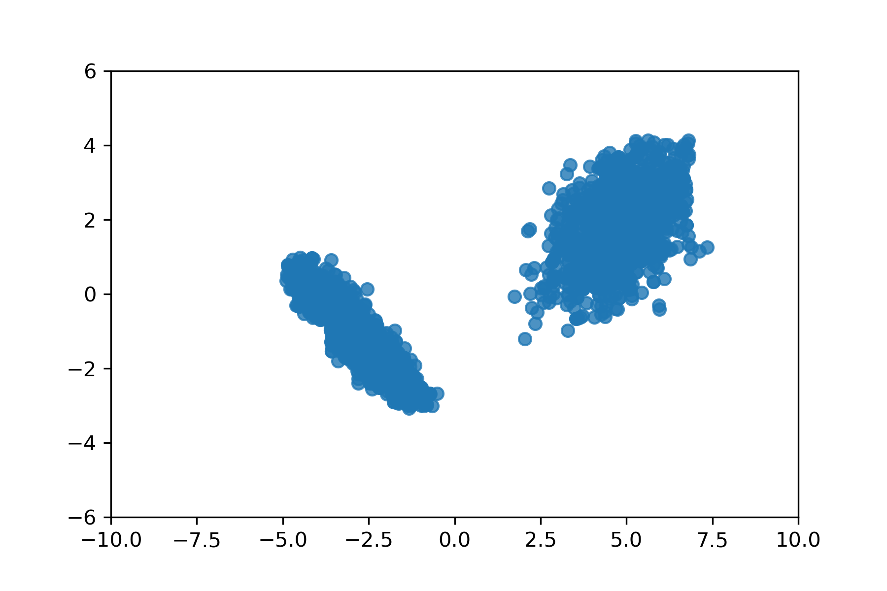
To illustrate this, we use an example of sampling the target form a two-component normal mixture in $\mathbb{R}^{2}$ : $\theta\sim 0.5\;N(\left(\begin{smallmatrix}-3\\ -1\end{smallmatrix}\right),\left(\begin{smallmatrix}1&-0.9\\ -0.9&1\end{smallmatrix}\right))+0.5\;N(\left(\begin{smallmatrix}5\\ 2\end{smallmatrix}\right),\left(\begin{smallmatrix}1&0.5\\ 0.5&1\end{smallmatrix}\right)).$ with uniform reference $\Pi_{r}(\beta)\sim\text{Uniform}\{(0,1)^{2}\}$ . After the optimization, we plot the randomly sampled $\beta$ and transported $\theta$ in Figure 2. Panel(a) shows the partitioning of the space using $\hat{c}$ . The logistic function help divide the space of $\beta$ into small local regions, where in each region, the points are most likely to go through $T_{\hat{c}}$ . Panels (b) and (c) show the randomly drawn $c$ for each point and the obtained sample $T_{c}(\beta)$ .

2.4 Transport to Discrete Posterior

Now we extend the transport plan to a discrete $\theta\sim\Pi(\theta;y)$ . Since the continuous transform is much more convenient to deal with, we use an embedding strategy by considering another continuous latent variable $\eta\in\mbox{\boldmath$\eta$}$ , such that its space $\eta$ can be partitioned into disjoint subsets $\{\mathcal{A}_{\theta}\}_{\theta}$ and each $\mathcal{A}_{\theta}$ corresponds to a unique value of $\theta$ . To give a concrete example, if our parameter of interest is binary $\theta=\{0,1\}$ , then we can use two intervals $\mathcal{A}_{0}=(-1,0)$ and $\mathcal{A}_{1}=(0,1)$ as the embedding sets. Since the subsets are disjoint, if we know $\eta$ , we can recover the corresponding $\theta$ via finding the enclosing set of $\eta$ , we denote this reverse lookup by $\theta=R(\eta)$ . In the above binary example, we can use $R(\theta)=\lceil\eta\rceil$ , the ceiling funciton. For a categorical $m\in\mathbb{Z}_{+}$ , one can similarly use $\mathcal{A}_{m}=(m-1,m)$ as the embedding. For more advanced examples, see Nishimura et al. 2020, Pakman and Paninski 2013.

Further, if we choose each $\mathcal{A}_{\theta}$ to have a unit volume, we can assign a uniform conditional density $\Pi(\eta\mid\theta)=1(\eta\in\mathcal{A}_{\theta})$ . This leads to the marginal density,

\displaystyle\Pi(\eta)=\sum_{\theta\in\Theta}\Pi(\theta;y)\Pi(\eta\mid\theta)=\sum_{\theta\in\Theta}\Pi(\theta;y)1(\eta\in\mathcal{A}_{\theta})=\Pi\{R(\eta);y\},

with its support $\{\eta:R(\eta)\in\Theta\}$ ; the summation disappears because for a given $\eta$ , $1(\eta\in A_{\theta})=1$ only when $\theta=R(\eta)$ , and is $0$ for $\theta\neq R(\eta)$ . We can now instead consider the random transport plan between $\eta$ and a continuous reference $\beta$ , and transform $\eta$ to $\theta$ later:

\displaystyle(\eta,\beta)\sim\Pi(\eta,\beta)\text{ such that}\hskip 10.00002pt\int_{\mbox{\boldmath$\beta$}}\Pi(\eta,\beta)\textup{d}\beta=\Pi(\eta),\int_{\mbox{\boldmath$\eta$}}\Pi(\eta,\beta)\textup{d}\eta=\Pi_{r}(\beta).

Similar to (2), we approximate the conditional $\Pi(\beta\mid\eta)$ by $\tilde{\Pi}(\beta\mid\eta)=\sum_{k=1}^{\infty}w_{k}(\eta)\delta\{\beta-T^{-1}_{k}(\eta)\},$ and integrating over $\eta$ gives the approximate marginal:

\displaystyle\tilde{\Pi}(\beta)=\sum_{k=1}^{\infty}w_{k}\{T_{k}(\beta)\}\Pi[R\{T_{k}(\beta)\};y]{|\textup{det}\nabla T_{k}(\beta)|}1\{T_{k}(\beta)\in\mbox{\boldmath$\eta$}\}.

After minimizing the difference between the $\tilde{\Pi}(\beta)$ and $\Pi_{r}(\beta)$ . Using $\beta\sim\Pi_{r}$ , the reverse conditional distribution for sampling $\theta$ is:

\displaystyle\tilde{\Pi}[\theta=R\{T_{k}(\beta)\}\mid\beta]=\frac{w_{k}\{T_{k}(\beta)\}\Pi[R\{T_{k}(\beta)\};y]{|\textup{det}\nabla T_{k}(\beta)|}1\{T_{k}(\beta)\in\mbox{\boldmath$\eta$}\}}{\sum_{k=1}^{\infty}w_{k}\{T_{k}(\beta)\}\Pi[R[\{T_{k}(\beta)\};y]{|\textup{det}\nabla T_{k}(\beta)|1\{T_{k}(\beta)\in\mbox{\boldmath$\eta$}\}}.}

In the data application, we will use this method to solve a challenging graph estimation problem. Due to the high similarity in methodology to the continuous cases, for conciseness, we will focus on continuous $\theta$ in the following discussion.

3 Transport Monte Carlo Algorithm

3.1 Algorithm

We design the Transport Monte Carlo (TMC) to be a two-stage algorithm: (i) optimization to estimate the working parameters in the mixture weights and location-scale transforms, (ii) sampling independent $\beta$ , and using the random transport to obtain $\theta$ . We keep those two stages separate since the optimization is the time-consuming step; given an estimated transport plan, the sampling is easy to carry out rapidly.

Optimization: With $\{w_{k},T_{k}\}_{k}$ fully parameterized, we can now minimize the Kullback-Leibler (KL) divergence $\mathbb{E}_{\beta\sim\Pi_{r}(\beta)}\log\{{\Pi_{r}(\beta)}/{\tilde{\Pi}(\beta)}\}$ , so that $\Pi_{r}(\beta)\approx\Pi(\beta)$ .

The total loss, including the Dirichlet process regularization on $b_{k}$ is

$\displaystyle Loss=$	$\displaystyle\mathbb{E}_{\beta\sim\Pi_{r}(\beta)}\log\{{\Pi_{r}(\beta)}/{\tilde{\Pi}(\beta)}\}-(\alpha/K-1)\sum_{k}\log b_{k}$	(8)
$\displaystyle=$	$\displaystyle-\mathbb{E}_{\beta\sim\Pi_{r}(\beta)}\log\sum_{k=1}^{K}w_{k}\{T_{k}(\beta)\}{L\{y;T_{k}(\beta)\}\Pi_{0}\{T_{k}(\beta)\}\ \prod_{j=1}^{p}s_{k,j}}1\{T_{k}(\beta)\in\Theta\}$
	$\displaystyle-\sum_{k=1}^{K}(\alpha/K-1)\log b_{k}+\text{constant},$

where the working parameters to optimize are $\{s_{k},m_{k},a_{k},b_{k}\}_{k}$ . To allow tractable computation, we use a truncation at $K$ , as an approximation to the infinite dimension Dirichlet distribution (Ishwaran and Zarepour 2002). This leads to an effective number of working parameters $K(3p+1)$ . In this article, we use $K=100$ in most of our examples.

To minimize the loss function, we use the stochastic gradient descent method. Since the expectation may be intractable, we draw a batch of $\beta_{l}\sim\Pi_{r}(\beta)$ for $l=1,\ldots,n_{b}$ , then calculate the gradient based on this batch and carry out a gradient descent step on the parameters; then we draw a new set of $\beta_{l}\sim\Pi_{r}(\beta)$ in the next step. Effectively, this is equivalent to the stochastic gradient descent on an infinitely large training sample, since we can draw infinitely many samples from $\Pi_{r}(\beta)$ . Such a method is routinely used in the variational inference (Kingma and Welling 2014), and prevents overfitting to the finite number of training samples. We provide more details on the optimization in the next subsection.

Drawing $\theta$ via Random Transport: After the optimization converges, the samples of $\theta$ can be obtained via

		$\displaystyle\beta\stackrel{{\scriptstyle iid}}{{\sim}}\Pi_{r},$
		$\displaystyle c\sim\text{Categorical}\{v_{1}(\beta),\ldots,v_{K}(\beta)\},$
		$\displaystyle\theta=T_{c}(\beta).$

Strictly speaking, the samples of $\theta$ generated from above are approximation to $\theta\sim\Pi(\theta;y)$ , since we substitute $\tilde{\Pi}(\beta)$ by $\Pi_{r}$ in the first line. As shown in all of our cases, we found the approximations indistinguishable from the ones obtained from a long-time run of MCMC.

3.2 Details on the Optimization

We now provide more details on the optimization stage on: (i) how to effectively optimize all $K$ components, especially in a high dimensional setting; (ii) how to diagnose if the selected $K$ is sufficiently large; and (iii) how to initialize the working parameters.

3.2.1 Component-wise Optimization

Since we approximate the infinite mixture components at a truncation $K$ , it would be desirable that those $K$ components contain most of the “effective” transforms for minimizing the divergence. To quantify the effectiveness, note that (8) contains a LogSumExp function

\text{LSE}(l_{1},\ldots,l_{K})=\log\{\sum_{k=1}^{K}\exp(l_{k})\}

where $l_{k}=\log[w_{k}\{T_{k}(\beta)\}{L\{y;T_{k}(\beta)\}\Pi_{0}\{T_{k}(\beta)\}\ \prod_{j=1}^{p}s_{k,j}}]-\chi_{\Theta}\{T_{k}(\beta)\}$ , with $\chi_{\Theta}(t)=0$ if $t\in\Theta$ and $\chi_{\Theta}(t)=\infty$ otherwise. If we reorder the $(l_{1},\ldots,l_{K})$ , $l_{(1)}\leq l_{(2)}\leq\ldots\leq l_{(K-h)}\leq l_{(K-h+1)}\leq\ldots\leq l_{(K)}$ , then we can bound this function from both sides:

l_{(K)}\leq\text{LSE}(l_{1},\ldots,l_{K})\leq l_{(K)}+\log h+\exp(l_{(K-h)}-l_{(K)})(K-h)/h,

where the lower bound is due to $\exp(l_{(K)})\leq\sum_{k=1}^{K}\exp(l_{k})$ , and the upper bound is due to $\sum_{k=1}^{K-h}\exp(l_{k})\leq(K-h)\exp(l_{(K-h)})$ and $\sum_{k=K-h+1}^{K}\leq h\exp(l_{(K)})$ , in addition to $\log(a+b)\leq\log a+b/a$ for $a>0,b>0$ . Now, note that if $l_{(K-h)}\ll l_{(K)}$ , then the last term is close to $0$ , hence the LSE function is almost fully determined by the top $h$ components that are close to $l_{(K)}$ . Therefore, with $l_{k}$ and $l_{(K)}$ dependent on $\beta$ , a useful score measuring the effectiveness of the component $k$ is $\xi_{k}=\mathbb{E}_{\beta\sim\Pi_{r}}\exp(l_{k}-l_{(K)})$ .

To see how this score impacts the gradient descent algorithm, we can compute the magnitude of the gradient with respect to the working parameters in the $k$ th component,

\|\nabla_{k}{\text{LSE}(l_{1},\ldots,l_{K})}\|=\frac{\exp(l_{k})}{\sum_{k^{\prime}=1}^{K}\exp(l_{k^{\prime}})}\|\nabla_{k}l_{k}\|\leq\exp(l_{k}-l_{(K)})\|\nabla_{k}l_{k}\|.

Now, if a component is initialized at $\exp(l_{k}-l_{(K)})\approx 0$ , then the gradient descent would almost not update the working parameters. This is very common when the parameters are in high dimension and randomly initialized.

Therefore, a component-wise optimization with a good initialization, is more useful than simultaneously updating all components. Specifically, for $k=1,\ldots,K$ ,

1.

Compute the scores: $\xi_{j}=\mathbb{E}_{\beta\sim\Pi_{r}}\exp(l_{j}-l_{(K)})$ using the samples of $\beta$ , for all $j=1,\ldots,K$ . Find the set of components with scores $H=\{j:\xi_{j}>\tau\}$ .
2.

Re-initialize the weak component: if the current $\xi_{k}<\tau$ , draw an index $j$ from $H$ , and set the parameters in $(T_{k},w_{k})$ to be equal to $(T_{j},w_{j})$ plus a small perturbation.
3.

Optimize the $k$ th component: optimize $(T_{k},w_{k})$ using the gradient descent until the empirical KL divergence converges, while keeping the other $(T_{k^{\prime}},w_{k^{\prime}})$ fixed.

In the implementation, we use a threshold $\tau=0.01$ and perturbation $N(0,0.01/p)$ to yield a good initialization for each component. During this process, we use the PyTorch framework for auto-differentiation and ADAM optimizer (Kingma and Ba 2014) for gradient descent. We consider each optimization converged if the change in the empirical KL divergence is smaller than a threshold of over $100$ iterations.

3.2.2 Diagnostics on $K$ and Convergence

At the same time, this strategy enables us to easily diagnose if the chosen $K$ is large enough. Note that the KL divergence is always greater or equal to zero, hence in the loss function (8), the function $-\mathbb{E}_{\beta\sim\Pi_{r}(\beta)}\text{LSE}(l_{1},\ldots,l_{K})$ is bounded from below at a constant [to be exact, the log of the normalizing constant $\log z(y)$ ]. Therefore, we can collect the optimized value every time we finish updating a component, creating a curve over $k=1,\ldots,K$ . If we see the curve flattening well before $K$ , then the selected $K$ is very likely to be sufficient; otherwise, we should increase $K$ . We provide an example diagnostic plot in the supplementary materials.

Remark 3.

One could extend our algorithm by indefinitely adding and optimizing a new component, until the KL divergence does not decrease any further. This could prevent the need to specify an upper bound $K$ . See Miller et al. 2017 for a similar algorithm.

3.2.3 Initialization

Since the loss function (8) is usually non-convex (for example, when the posterior density is non-convex), it is helpful to use a good initialization on the working parameters. With $\Pi_{r}$ chosen as the $\text{Uniform}\{(0,1)^{p}\}$ , we set all $a_{k}$ and $b_{k}$ to be zero in the logistic function so that the initial weights are all equal, and the shift parameters $m_{k}$ to be in the high posterior density region of $\theta$ . For the target distribution with log-concave density, we can first calculate the posterior mode $\hat{\theta}$ using optimization, then generate $m_{k}$ ’s near $\hat{\theta}$ . On the other hand, this is more difficult for the multi-modal target distribution, especially when the modes are far apart; in such a case, we randomly generate $m_{k}$ ’s uniformly in an estimated range of $\theta$ , then rely on the mixture framework for the parallel searches for all the modes. We found this strategy yield good empirical performance, as demonstrated in the example of sampling a target posterior with $25$ modes in the supplementary materials — although in more sophisticated cases, some customized initialization should be used instead.

3.3 Combining with Independence Hastings Algorithm

As in the other popular approaches, there are approximation errors incurred in the TMC algorithm, for example, due to the use of finite $K$ , the $\epsilon$ -suboptimal convergence of the optimization, etc. Since such errors are often intractable, some control methods are needed.

For this purpose, we develop an extension to combine TMC with the independence Hastings algorithm. For conciseness of presentation, we defer the method to the supplementary materials.

4 Theoretic Study

In this section, we give a more theoretical exposition on the TMC method. For the mathematic rigor, we will focus on $\Pi(\theta;y)$ being the posterior density corresponding to $\{\Theta,\mathcal{B}(\Theta),\mu\}$ , with $\Theta\subseteq\mathbb{R}^{p}$ , $\mathcal{B}$ the Borel $\sigma$ -algebra and $\mu$ absolutely continuous with respect to the Lebesgue measure.

Before presenting results, we use a simple example to show the intuition of “changing one histogram into another”, behind the choice of uniform distribution for $\Pi_{r}$ and location-scale transformation for $T_{k}$ ’s. Suppose that we want to find an approximate transport plan between $\beta\sim U(0,1)$ and $\theta\sim N(0,1)$ , a standard normal distribution: we first find the high density region of $\theta$ , divide it into disjoint bins (denoted by $\Theta_{j}$ ’s), compute the probability within each bin [denoted by $\text{pr}_{\theta}(\Theta_{j})$ ] and re-normalize them so that $\sum_{j}\text{pr}_{\theta}(\Theta_{j})=1$ . As a result, this produces the commonly used histogram, where we replace the density within each bin by a flat constant (therefore, leading to an approximation). Similarly, we divide the support of the uniform $(0,1)$ into multiple bins (denoted by $\mbox{\boldmath$\beta$}_{k}$ ’s), and obtain corresponding probabilities $\text{pr}_{\beta}(\mbox{\boldmath$\beta$}_{k})$ ’s.

With these two marginal histograms, we can find a joint distribution $\text{pr}_{\theta,\beta}(\Theta_{j},\mbox{\boldmath$\beta$}_{k})$ , such that $\sum_{k}\text{pr}_{\theta,\beta}(\Theta_{j},\mbox{\boldmath$\beta$}_{k})=\text{pr}_{\theta}(\Theta_{j})$ and $\sum_{j}\text{pr}_{\theta,\beta}(\Theta_{j},\mbox{\boldmath$\beta$}_{k})=\text{pr}_{\beta}(\mbox{\boldmath$\beta$}_{k})$ — that is, solving for a contingency table with known marginal values. Obviously, there are more than one solutions. We plot a solved table of $\text{pr}_{\theta,\beta}(\Theta_{j},\mbox{\boldmath$\beta$}_{k})$ in Figure 3 with $30$ bins for $\theta$ and $30$ bins for $\beta$ . To show more details in each table cell, we also solved for a smaller table (Table 1 in the supplementary materials) with $6$ bins for $\theta$ and $2$ bins for $\beta$ .

Note that these solutions are sparse with some $pr_{\theta,\beta}(\Theta_{j},\mbox{\boldmath$\beta$}_{k})=0$ . And in each $(\Theta_{j},\mbox{\boldmath$\beta$}_{k})$ , we can impose a one-to-one transform $\theta=T_{l}(\beta)$ that changes a uniform distribution in $\mbox{\boldmath$\beta$}_{k}$ to a uniform distribution in $\Theta_{j}$ — clearly, the simple scale-location change $T_{l}$ is adequate for this task. As the number of bins $\Theta_{j}$ ’s increases, we can expect the histogram to converge to the target density of $\theta$ . We now formalize this intuition.

Without loss of generality, we use $\beta\sim\text{Uniform}(0,1)^{p}$ ; after the location-scale change, the transformed follows $T_{k}(\beta)\sim\text{Uniform}\{\times_{j=1}^{p}(m_{k,j},s_{k,j}+m_{k,j})\}$ . The density of (5) at a specific value $\theta_{0}$ is:

	$\displaystyle\tilde{\Pi}(\theta_{0})$	$\displaystyle=\int\Pi_{r}(\beta)\sum_{k=1}^{K}v_{k}(\beta)\delta\{\theta_{0}-T_{k}(\beta)\}\textup{d}\beta$
		$\displaystyle=\sum_{k=1}^{K}v_{k}\{T^{-1}_{k}(\theta_{0})\}\frac{1}{\prod_{j=1}^{p}s_{k,j}}1\{T^{-1}_{k}(\theta_{0})\in(0,1)^{p}\},$

where we exchange the summation and integral, and use $\int_{X}f(x)\delta(x-y)\textup{d}x=f(y)1(y\in X)$ . Rewriting this as

		$\displaystyle\tilde{\Pi}_{K}(\theta_{0})=\sum_{k=1}^{K}\tilde{a}_{k}(\theta_{0})1(\theta_{0}\in C_{k}),$		(9)
		$\displaystyle\tilde{a}_{k}(\theta_{0})=\frac{v^{*}_{k}(\theta_{0})}{\prod_{j=1}^{p}s_{k,j}},C_{k}=\times_{j=1}^{p}(m_{k,j},s_{k,j}+m_{k,j}),$		(9)

where $v^{*}_{k}(\theta_{0})=v_{k}\{s_{k}^{-1}\odot(\theta_{0}-m_{k})\}$ . Note that if we had $\Pi^{*}_{K}(\theta_{0})=\sum_{k=1}^{K}\tilde{a}_{k}1(\theta_{0}\in C_{k})$ with $\tilde{a}_{k}$ does not depend on $\theta_{0}$ , then $\Pi^{*}_{K}(\theta_{0})$ would be a “simple function”. The simple function is routinely used for approximating any Lebesgue-measurable function, as stated in the following theorem.

Theorem 1.

(Schilling 2017) Let $\{\Theta,\mathcal{B}(\Theta)\}$ be a measurable space, and $f$ be a measurable function. Then there exists a sequence $\left({f_{K}}\right)_{K\in\mathbb{Z}_{+}}$ , with each $f_{K}$ a simple function, such that, $\forall\theta_{0}\in\Theta:f\left({\theta_{0}}\right)=\displaystyle\lim_{K\to\infty}f_{K}\left({\theta_{0}}\right)$ .

On the other hand, now since each $\tilde{a}_{k}(\theta_{0})$ does depend on $\theta_{0}$ , with $\tilde{a}_{k}(\theta)$ set by a specific form of $v_{k}(\theta)$ as in (4). Therefore, some additional work is needed to show a similar asymptotic result. We state the result as followed and provide a construction in the proof. For conciseness, we provide all the proofs in the supplementary materials.

Theorem 2.

Let $\Theta\subseteq\mathbb{R}^{p}$ be the set for $0<\Pi(\theta;y)<\infty$ , if $\Pi(\theta;y)$ is a continuous function in $\Theta$ except for finite number of points, then there exists a sequence $({\tilde{\Pi}_{K}})_{K\in\mathbb{Z}_{+}}$ , with each ${\tilde{\Pi}_{K}}$ in the form of (9), such that, $\Pi(\theta;y)=\displaystyle\lim_{K\to\infty}\tilde{\Pi}_{K}(\theta)$ almost everywhere in $\Theta$ .

Next, we focus on the random transport plan (1), as the joint probability betweena $\theta$ and $\beta$ . Recall that we obtain its estimate via discretizing the conditional $\Pi(\beta\mid\theta)$ using a mixture and matching its marginal $\tilde{\Pi}(\beta)$ to a chosen $\Pi_{r}(\beta)$ . We want to show that there exists solution for $\{(w_{k},T_{k})\}_{k}$ with negligibly small difference. To formalize, let $P_{0}(\theta,\beta)$ be a joint density of $\theta$ and $\beta$ , that has the marginals exactly as $\beta\sim\text{Uniform}\{(0,1)^{p}\}$ and $\theta\sim\Pi(\theta;y)$ . For a measurable $\mathcal{A}\in\mathcal{B}(\mbox{\boldmath$\beta$})$ with $\mbox{\boldmath$\beta$}=(0,1)^{p}$ , denote the conditional measure by

\displaystyle\nu_{\beta\mid\theta}(\mathcal{A})=\int_{\mathcal{A}}\frac{P_{0}(\theta,\beta)}{\Pi(\theta;y)}\textup{d}\beta\in(0,1].

Since there exists more than one $P_{0}(\theta,\beta)$ , we can focus on those with $\nu_{\beta\mid\theta}$ corresponding to a measure absolutely continuous with respect to a Lebesgue measure.

Theorem 3.

Denote the measures corresponding to $\Pi_{r}(\beta)$ and $\tilde{\Pi}(\beta)$ by $\pi_{r}$ and $\tilde{\pi}_{\beta}$ , respectively. If $P_{0}(\theta,\beta)$ satisfies that $\nu_{\beta\mid\theta}$ is absolutely continuous with respect to the Lebesgue measure for any $\|\theta\|_{2}<\infty$ , then there exists a sequence $\{w_{k},T_{k}\}_{k=1}^{K}$ with $T_{k}$ parameterized by location-scale transform (6) and $w_{k}:w_{k}(\theta)\geq 0,\sum_{k=1}^{K}w_{k}(\theta)=1$ , such that the total variation distance

\lim_{K\to\infty}\sup_{\mathcal{A}\in\mathcal{B}(\mbox{\boldmath$\beta$})}|\pi_{r}(\mathcal{A})-\tilde{\pi}_{\beta}(\mathcal{A})|=0.

Strictly speaking, in the above we consider a broad class of functions $w:\Theta\to\Delta^{K-1}$ , with $\Delta^{K-1}$ the probability simplex.

We now turn to the algorithmic details of the TMC. As suggested in the last theorem, under a large $K$ , we can expect $\tilde{\pi}(\beta_{l})$ to be close to $\pi_{r}(\beta_{l})$ for most of the samples $\beta_{l}$ ’s generated during the optimization. On the other hand, since $(0,1)^{p}$ is a continuous space, there are always points that we have not trained on — if we generate a new $\beta^{*}$ and sample $\theta^{*}$ through (5), how can we guarantee that it still has a low approximation error?

Since we use stochastic gradient descent with batch size $n_{b}$ , by the time when we stop after $t$ iterations, the optimization is effectively based on $n=n_{b}t$ training samples. Intuitively, if the training $\{\beta_{l}\}_{l=1}^{n}$ are “dense” enough to cover most of $(0,1)^{p}$ — that is, the maximal spacing $\max_{i}\min_{j}\|\beta_{i}-\beta_{j}\|$ is small, any new sample $\beta^{*}$ drawn in the sampling stage will be near a certain training $\beta_{l}$ ; hence, the associated $\tilde{\Pi}(\beta^{*})$ should be very close to $\Pi(\beta_{l})$ (on the logarithmic scale, as in the optimization). The following theorem formalizes this intuition and quantifies how the error vanishes in terms of $n$ .

Theorem 4.

If $\Pi(\theta;y)$ is absolutely continuous, then

\displaystyle\inf_{l\in\{1\ldots n\}}\|\log\tilde{\Pi}(\beta^{*})-\log\tilde{\Pi}(\beta_{l})\|=\mathcal{O}\{\ \frac{p(2\log\log n+\log n)}{n}\}.

This above rate is due to the uniform reference $\Pi_{r}(\beta)$ having a compact support; hence the maximal spacing drops to zero rapidly in a roughly $\mathcal{O}(1/n)$ rate. For the other reference with unbounded support, such as multivariate normal, we would not have such a guarantee. In fact, the rate based on a normal $\Pi_{r}(\beta)$ would be approximately $\mathcal{O}(1/\sqrt{\log n})$ (Deheuvels et al. 1986), substantially slower than uniform.

5 Comparison with the Hamiltonian Monte Carlo

With the augmented random variable $\beta\in\mathbb{R}^{p}$ and the deterministic transforms, the TMC may appear similar to the popular Hamiltonian Monte Carlo (HMC) algorithm. Therefore, it is interesting to compare those two methods.

To provide some background, the HMC uses an augmented “momentum” variable $v\in\mathbb{R}^{p}$ , with $v\sim\Pi(v)$ (independent from $\theta$ in the original HMC algorithm (Neal 2011), or dependent on $\theta$ in the Riemannian manifold HMC, RMHMC (Girolami and Calderhead 2011)). With $\Pi(\theta,v)=\exp\{-H(\theta,v)\}$ , $H(\theta,v)$ is referred to as the Hamiltonian. For multiple copies of $(\theta,v)$ indexed over time $t\in[0,\infty)$ , denoted by $\{(\theta^{t},v^{t})\}_{t}$ , they change smoothly according to the Hamilton’s equations:

\displaystyle\frac{\partial\theta^{t}}{\partial t}=\frac{\partial H(\theta^{t},v^{t})}{\partial v^{t}},\hskip 20.00003pt\frac{\partial v^{t}}{\partial t}=-\frac{\partial H(\theta^{t},v^{t})}{\partial\theta^{t}}.

(10)

Using one Markov chain sample of $(\theta,v)$ as the initial $(\theta^{0},v^{0})$ , one could obtain another sample $(\theta^{T},v^{T})$ at time $T$ , deterministically using the exact solution to (10). On the other hand, for most of the posterior densities, the equation (10) cannot be solved in closed form; therefore, some approximation is often used, such as the leapfrog scheme: $\theta^{t+\varepsilon/2}=\theta^{t}+(\varepsilon/2){\partial H(\theta^{t},v^{t})}/{\partial v^{t}}$ , and $v^{t+\varepsilon/2}=v^{t}-(\varepsilon/2){\partial H(\theta^{t},v^{t})}/{\partial\theta^{t}}$ for $t=0,\varepsilon/2,\ldots,\varepsilon L$ , and then $(\theta^{T},v^{T})$ at $T=\varepsilon L$ is accepted/rejected using the Metropolis-Hastings step. When $L=1$ , the above is equivalent to the Metropolis-adjusted Langevin Algorithm (MALA). Now, to compare them with the TMC:

1.

From the perspective of transport, both the exact and approximate solutions to the Hamilton’s equations (before the Metropolis-Hastings correction) can be viewed as a transport plan from $(\theta^{0},v^{0})$ to $(\theta^{T},v^{T})$ . That is, it forms a joint distribution among $(\theta^{0},v^{0},\theta^{T},v^{T})$ — importantly, although $\theta^{0}$ and $v^{0}$ can be independent, across time, $\theta^{T}$ is dependent on $v^{0}$ , and $v^{T}$ is dependent on $\theta^{0}$ . In comparison, the TMC focus on one copy of $(\theta,\beta)$ , with a dependency in between; across two copies, $(\theta^{i},\beta^{i})$ are independent from $(\theta^{i^{\prime}},\beta^{i^{\prime}})$ for $i^{\prime}\neq i$ .
2.

In terms of the computation burden, in the HMC, the transformation from $(\theta^{0},v^{0})\to(\theta^{T},v^{T})$ is pre-determined as the solution to (10), but due to the often lack of closed-form, some intensive and iterative algorithm (such as the leapfrog) is needed to produce a new $\theta^{T}$ relatively far away from the current $\theta^{0}$ . In the TMC, the transformation $\beta\to\theta$ is not known beforehand and needs to be estimated, but after the optimization, the transformation is simple to compute.
3.

In both approaches, a Metropolis-Hastings step would be needed to correct the numeric errors, so that the sample collected can converge to the target posterior distribution as the number of samples diverges.

To illustrate the above points, we use the two-component normal mixture in $\mathbb{R}^{2}$ as the target distribution [Figure 4(a)]: $\theta\sim N[\left(\begin{smallmatrix}5\\ -1\end{smallmatrix}\right),\left(\begin{smallmatrix}1&-0.9\\ -0.9&1\end{smallmatrix}\right))+0.5\;N(\left(\begin{smallmatrix}5\\ 2\end{smallmatrix}\right),\left(\begin{smallmatrix}1&0.9\\ 0.9&1\end{smallmatrix}\right)].$ This modifies the previous example by bringing the two components means closer to each other, so that the HMC can visit both components more easily. We initialized each algorithm at one of the means $\hat{\theta}=[5,2]$ , and tuned each algorithm to have the acceptance rate close to $70\%$ . We ran each HMC algorithm for $20,000$ steps.

Since $\theta_{2}$ has two local optima at $-1$ and $2$ , we can use its traceplot to visualize how quickly each algorithm can jump from one normal component to another. Among the HMC algorithms, the MALA was the fastest to run (due to $L=1$ in the numeric approximation, it took $36$ seconds) but suffered from high autocorrelation, as each new proposal is very close to the current one (panel c); the HMC with No-U-Turn sampler (HMC-NUTS) had a much lower autocorrelation (panel e), although at a much higher computational cost (it took $1260$ seconds to run, with each new proposal taking on average $L=53$ steps to generate). In addition, we tested the Riemannian manifold HMC (RMHMC), which makes the covariance matrix of $v$ depend on the current state of $\theta$ via the observed Fisher information (Girolami and Calderhead 2011), hence potentially giving better adaptation to the local geometry of the high posterior density region. We set $L=1$ in RMHMC and found a much better performance than the MALA. However, since each step was computationally intensive [we used the state-of-art explicit-scheme integrator (Cobb et al. 2019) that improves upon the implicit-scheme one (Girolami and Calderhead 2011) in speed], it took a longer time (1800 seconds) and was less efficient in exploring two components (panel d), compared to the HMC-NUTS. To summarize, the HMC-NUTS algorithm was the most efficient among all the HMC algorithms in this experiment.

To compare, the TMC took 18 seconds to optimize and less than 1 second to generate $20,000$ samples. We further applied the Metropolis-Hastings step on the generated samples, which lead to an acceptance rate of $90\%$ . As a result, the produced samples were almost independent.

In addition, we carried out experiments on: (i) the estimation of high-dimensional regression using the shrinkage prior, (ii) sampling from multi-modal distribution, (iii) comparing the performance with various normalizing flow neural networks. The details are provided in the supplementary materials.

6 Application: Graph Estimation under Degree Regularization

We now illustrate the performance of discrete parameter estimation using a data application. The data are the multivariate electroencephalogram (EEG) time series collected over $V=128$ electrodes when the human subject is performing a working memory task. Our goal is to estimate an undirected graph $G=\{\mathcal{V},\mathcal{E}\}$ with $\mathcal{V}=\{1,\ldots,V\}$ the nodes and $E=\{e_{i,j}\}$ the edges, based on the temporal correlation among those time series. The parameter of the interest is a binary adjacency matrix $A=\{A_{i,j}\}$ , with $A_{i,j}=1$ if $e_{i,j}\in E$ , $0$ otherwise for $j<i$ ; $A_{j,i}=A_{i,j}$ and we fix $A_{i,i}=0$ . In particular, we are interested in finding a subset of nodes that are well connected during this memory task, while excluding the remaining as isolated singletons. Therefore, it is useful to consider a prior shrinkage on the graph degree $D_{i}=\sum_{j\neq i}A_{i,j}$ for $i=1\ldots,V$ .

To prescribe a likelihood for graph estimation, we are motivated by the popularity of the simple hard-thresholding on the empirical correlation matrix $A_{i,j}=1(|\rho_{i,j}|>\tau)$ with some $\tau\in(0,1)$ . Although appearing heuristic, it was recently shown to have an equivalence to the more sophisticated graphical lasso (Sojoudi 2016). Therefore, it is interesting to develop a generalized Bayes extension that allows prior regularization. Assuming $|\rho_{i,j}|\neq 0$ or $1$ , we assign a Beta pseudo-likelihood for each $|\rho_{i,j}|$ and a degree shrinkage-prior,

		$\displaystyle L(\rho_{i,j};A_{i,j})\propto\|\rho_{i,j}\|^{A_{i,j}}(1-\|\rho_{i,j}\|)^{(1-A_{i,j})}\text{ for }j<i,$
		$\displaystyle\Pi_{0,A}(A)\propto\prod_{i=1}^{V}(\phi_{i}\tau)^{-1}\exp(-\frac{D_{i}}{\phi_{i}\tau}),$
		$\displaystyle\Pi_{0,\phi}(\phi)\propto\prod_{i=1}^{V}\phi^{\alpha-1}_{i},\hskip 20.00003pt\Pi_{0,\tau}(\tau)\propto\exp(-\frac{\tau}{V}).$

Each $A_{i,j}$ can be viewed as if a Bernoulli random variable and therefore a “soft” thresholding. Note that although it ignores the positive definite constraint for the correlation matrix, this generalized Bayes posterior still enjoys coherence in decision theory, as studied by Bissiri et al. 2016. For the prior, we use the Dirichlet-Laplace shrinkage prior (Bhattacharya et al. 2015) for the degrees $(D_{1},\ldots,D_{V})$ , with $\phi\sim\text{Dirichlet}(\alpha,\ldots,\alpha)$ , $\tau\sim\text{Exp}(V)$ with a weakly-informative mean at $V$ . We use $\alpha=0.01$ to encourage sparsity in $(\phi_{1},\ldots,\phi_{V})$ .

In this case, the parameter is in high dimension $p=8,193$ , and we have both continuous and discrete elements. To accommodate this, we separate the output of each $T_{k}(\beta)$ into three parts $(\gamma^{k}_{1},\gamma^{k}_{2},\gamma^{k}_{3})$ , corresponding to $(A,\phi,\tau)$ , and use

\tilde{\Pi}(\beta)\propto\sum_{k=1}^{K}w_{k}\big\{T_{k}(\beta)\big\}{|\textup{det}\nabla T_{k}(\beta)|}\Pi_{0,\phi}(\gamma^{k}_{2})\Pi_{0,\tau}(\gamma^{k}_{3})\prod_{j<i}L\{\rho_{i,j};R(\gamma^{k}_{1})\}\Pi_{0,A}\{R(\gamma^{k}_{1})\},

where $\Pi_{0,\phi}(\gamma^{k}_{2})$ is the Dirichlet density re-parameterized as the transform from gamma random variables Gamma $(\alpha,1)$ , multiplied to the associated Jacobian.

Figure 5 shows the result of posterior estimation. We successfully shrunk the degrees of some nodes to zero (panel d). The remaining nodes correspond to well-connected sub-graphs (panel c). To compare, we also ran graphical lasso, and it discovered a similar structure (panel b), except that it did not have degree-sparsity and under-estimated the large signals (as a known side-effect of the $l_{1}$ -regularization). For comparison, we ran the Gibbs sampling algorithm that updated one $A_{i,j}$ at a time. The mixing was extremely slow, as shown in Figure 5(e). The TMC was free from this issue as the samples were independent.

7 Discussion

In recent years, it has become increasingly easier to develop and apply Bayesian models, thanks to the new tools capable of handling posterior without closed-form conditional. A primary factor that contributes to their success is arguably the reduction of efforts and time needed for deriving and implementing an algorithm; as a result, statisticians can focus more on model design and calibration.

We believe our proposed method is another advance in this direction. In particular, our method substantially reduces the time needed from writing a Bayesian model to collecting posterior samples in the high probability region. In all of our experiments, including the high dimensional ones, the computation took at most a few minutes. Such a close to real-time feedback is very beneficial, and it encourages statisticians to explore new forms of likelihood and prior through rapid experiments. For example, our new regularized graph estimation was made possible because of the ability to avoid sequential search in the graph space, which would be a highly combinatorial and challenging problem.

Compared to the other optimization-based approaches, the main distinction of our proposal is the infinite mixture of simple transforms. This not only enables a “shotgun” algorithm that can handle multi-modality in the posterior, but also leads to a tractable theoretic analysis via piecewise probability approximation.

Lastly, this framework can be extended for general statistical inferences, such as the conditional density estimation. For example, one could estimate a transport plan between the empirical distributions of some predictors and an outcome of interest. This is similar to the estimation of Wasserstein distances (Solomon et al. 2015; Kolouri et al. 2019); nevertheless, to prevent overfitting under a finite sample size, it would be important to choose an appropriate cost function or regularization to yield a parsimonious transport plan. The methodology, as well as the signal recovery theory, is still an underexplored but interesting topic.

Acknowledgement

The author would like to thank James Hobert, David Dunson, and Yun Yang for useful discussions.

Supplementary Materials

Extension: Independence Hastings Algorithm

A unique advantage of Markov chain Monte Carlo (MCMC) is the “asymptotic exactness”: as the number of collected samples increases to infinity, under some conditions, the empirical distribution of the Markov chain samples will converge to the posterior distribution (Roberts and Tweedie 1996). Since the optimized random transport can generate samples with small approximation errors, we can use it to build a proposal-generating distribution. In the Markov chain, we denote a given state by $(\beta^{t},\theta^{t})$ with $\theta^{t}=T_{c^{t}}(\beta^{t})$ , and the new proposal by $(\beta^{*},\theta^{*})$ . To compare, the transport map-based MCMC algorithm (Parno and Marzouk 2018) transforms a simple Metropolis proposal $Q(\beta^{*}\mid\beta^{t})$ on the reference into a sophisticated one $Q(\theta^{*}\mid\theta^{t})$ for the target, hence the proposal is dependent on the current state; whereas in our extension, the proposal is independent $Q(\beta^{*},\theta^{*}\mid\beta^{t},\theta^{t})=Q(\beta^{*},\theta^{*})$ hence potentially more efficient in exploring the parameter space.

To formalize, consider the target distribution as the augmented $\Pi(\theta;y)\tilde{\Pi}(\beta\mid\theta)$ , with the later a categorical distribution $\text{Pr}\{\beta=T^{-1}_{k}(\theta)\}=w_{k}(\theta)$ as defined in the main text (except that we use the truncation at $K$ and treat the $\{T_{k},w_{k}\}_{k}$ as fixed). Clearly, the $\theta$ -marginal distribution is still the posterior $\Pi(\theta;y)$ .

When devising the proposal kernel, we recognize that if the target state space $\Theta$ is unbounded, such as $\mathbb{R}^{p}$ , there will be a small discrepancy from the image of $T_{k}$ ’s from a uniform reference sample $\beta\sim\Pi_{r}(\beta)$ . To correct this, we now generate the $\beta$ from a two-component mixture, with one component from uniform $\Pi_{r}(\beta)$ and the other from distribution $\Pi_{a}(\beta)$ with the unbounded support. This leads to a proposal kernel:

		$\displaystyle Q(\beta^{},\theta^{})=\{\rho\Pi_{r}(\beta^{})+(1-\rho)\Pi_{a}(\beta^{})\}\tilde{\Pi}(\theta^{}\mid\beta^{})$
		$\displaystyle=\{\rho\Pi_{r}(\beta^{})+(1-\rho)\Pi_{a}(\beta^{})\}$
		$\displaystyle\times\frac{w_{c}\{T_{c}(\beta^{})\}\Pi\{T_{c}(\beta^{});y\}{\|\textup{det}\nabla T_{c}(\beta^{})\|1\{\theta^{}=T_{c}(\beta^{}),T_{c}(\beta^{})\in\Theta\}}}{\sum_{k=1}^{K}w_{k}\{\ T_{k}(\beta^{})\}\ \Pi\{T_{k}(\beta^{});y\}{\|\textup{det}\nabla T_{k}(\beta^{})\|1\{T_{k}(\beta^{})\in\Theta\}}},$

with $\rho\in(0,1]$ and chosen to be a value close to $1$ . Using the Hastings algorithm, we accept $(\beta^{*},\theta^{*})$ with probability

\displaystyle\min\left\{1,\frac{\Pi(\theta^{*};y)\tilde{\Pi}(\beta^{*}\mid\theta^{*})}{\Pi(\theta^{t};y)\tilde{\Pi}(\beta^{t}\mid\theta^{t})}\frac{Q(\beta^{t},\theta^{t})}{Q(\beta^{*},\theta^{*})}\right\},

Applying change of variable $\theta=T_{c}(\beta)$ and some cancellations (detail provided later), the above acceptance rate becomes

\displaystyle\min\left[1,\frac{\{\rho\Pi_{r}(\beta^{t})+(1-\rho)\Pi_{a}(\beta^{t})\}\tilde{\Pi}(\beta^{*})|\textup{det}\nabla T_{c^{t}}(\beta^{t})|}{\{\rho\Pi_{r}(\beta^{*})+(1-\rho)\Pi_{a}(\beta^{*})\}\tilde{\Pi}(\beta^{t})|\textup{det}\nabla T_{c^{*}}(\beta^{*})|}1\{T_{c^{*}}(\beta^{*})\in\Theta\}\right].

Recall that $\tilde{\Pi}(\beta)$ is an approximation to $\Pi_{r}(\beta)$ — a uniform. Therefore, with $\rho\approx 1$ and $\{T_{k},w_{k}\}_{k}$ optimized, the acceptance rate will be close to a constant. Further, if we can ensure the $\textup{det}\nabla T_{k}(\beta)=\prod_{j=1}^{p}s_{k,j}$ is similar for all $k$ , then the acceptance rate will be close to one.

Remark 4.

Note that the proposal $(\theta^{*},\beta^{*})$ is independent of the current state $(\theta^{t},\beta^{t})$ , making this an independence Hastings algorithm (Tierney 1994).

As shown in early work [Tierney 1994; Mengersen and Tweedie 1996 among others], a sufficient condition to ensure asymptotic exactness of MCMC, is when the ratio between the proposal and target is bounded from below. In our case, this can be achieved with $\Pi_{a}(\beta)/\Pi[T_{k}(\beta);y]>\lambda$ for all $k=1,\ldots,K$ . To see this,

	$\displaystyle\frac{Q(\beta,\theta)}{\Pi(\theta;y)\tilde{\Pi}(\beta\mid\theta)}$	$\displaystyle=\frac{\{\rho\Pi_{r}(\beta)+(1-\rho)\Pi_{a}(\beta)\}\|\textup{det}\nabla T_{c}(\beta)\|\ }{\sum_{k=1}^{K}w_{k}\{T_{k}(\beta)\}\Pi\{T_{k}(\beta);y\}{\|\textup{det}\nabla T_{k}(\beta)\|1\{T_{k}(\beta)\in\Theta\}}}$		(11)
		$\displaystyle\geq(1-\rho)\lambda(\min_{l=1\ldots,K}\prod_{j=1}^{p}s_{l,j})/(\sum_{k=1}^{K}\prod_{j=1}^{p}s_{k,j}),$		(11)

due to the cancellation $\tilde{\Pi}\{\beta=T_{c}(\beta)\mid\theta\}=w_{c}\{T_{c}(\beta)\}$ , and $\Pi(\theta;y)=\Pi\{T_{c}(\beta);y\}$ , $\rho\Pi_{r}(\beta)>0$ and each $w_{k}\{T_{k}(\beta)\}\leq 1$ . In practice, a common choice for $\Pi_{a}(\beta)$ is a heavy-tail distribution, such as multivariate $t$ -distribution (provided it can satisfy the above condition). Another potential issue is that as the dimension $p\to\infty$ , the independence Hastings algorithm could suffer from the curse of dimensionality, with the acceptance rate approaching $0$ . A common remedy is to use block-wise updating, that each time proposes change to only one part of the parameter.

Details of Hastings Acceptance Rate

At the current state, $T_{c^{t}}(\beta^{t})\in\Theta$ ; if $T_{c^{*}}(\beta)\not\in\Theta$ , we will reject it; therefore, we focus on $T_{c^{*}}(\beta^{*})\in\Theta$ as well.

		$\displaystyle\frac{\cancel{\Pi(\theta^{};y)}\tilde{\Pi}(\beta^{}\mid\theta^{})}{\cancel{\Pi(\theta^{t};y)}\tilde{\Pi}(\beta^{t}\mid\theta^{t})}\frac{\{\rho\Pi_{r}(\beta^{t})+(1-\rho)\Pi_{a}(\beta^{t})\}\frac{w_{c^{t}}\{T_{c^{t}}(\beta^{t})\}\cancel{\Pi\{T_{c^{t}}(\beta^{t});y\}}{{\|\textup{det}\nabla T_{c^{t}}(\beta^{t})\|}}1\{\theta^{t}=T_{c^{t}}(\beta^{t}),T_{c^{t}}(\beta^{t})\in\Theta\}}{\sum_{k=1}^{\infty}w_{k}\{T_{k}(\beta^{t})\}\Pi\{T_{k}(\beta^{t});y\}{\|\textup{det}\nabla T_{k}(\beta^{t})\|1\{T_{k}(\beta^{t})\in\Theta\}}}}{\{\rho\Pi_{r}(\beta^{})+(1-\rho)\Pi_{a}(\beta^{})\}\frac{w_{c^{}}\{T_{c^{}}(\beta^{})\}\cancel{\Pi\{T_{c^{}}(\beta^{});y\}}{{\|\textup{det}\nabla T_{c^{}}(\beta^{})\|}}1\{\theta^{}=T_{c^{}}(\beta^{}),T_{c^{}}(\beta^{})\in\Theta\}}{\sum_{k=1}^{\infty}w_{k}\{T_{k}(\beta^{})\}\Pi\{T_{k}(\beta^{});y\}{\|\textup{det}\nabla T_{k}(\beta^{})\|1\{T_{c^{}}(\beta^{})\in\Theta\}}}}$
		$\displaystyle=\frac{\cancel{\tilde{\Pi}(\beta^{}\mid\theta^{})}}{\cancel{\tilde{\Pi}(\beta^{t}\mid\theta^{t})}}\frac{\{\rho\Pi_{r}(\beta^{t})+(1-\rho)\Pi_{a}(\beta^{t})\}\frac{\cancel{w_{c^{t}}\{T_{c^{t}}(\beta^{t})\}}{{\|\textup{det}\nabla T_{c^{t}}(\beta^{t})\|}}1\{\theta^{t}=T_{c^{t}}(\beta^{t})\}}{\sum_{k=1}^{\infty}w_{k}\{T_{k}(\beta^{t})\}\Pi\{T_{k}(\beta^{t});y\}{\|\textup{det}\nabla T_{k}(\beta^{t})\|1\{T_{k}(\beta^{t})\in\Theta\}}}}{\{\rho\Pi_{r}(\beta^{})+(1-\rho)\Pi_{a}(\beta^{})\}\frac{\cancel{w_{c^{}}\{T_{c^{}}(\beta^{})\}}{{\|\textup{det}\nabla T_{c^{}}(\beta^{})\|}}1\{\theta^{}=T_{c^{}}(\beta^{})\}}{\sum_{k=1}^{\infty}w_{k}\{T_{k}(\beta^{})\}\Pi\{T_{k}(\beta^{});y\}{\|\textup{det}\nabla T_{k}(\beta^{})\|1\{T_{c^{}}(\beta^{*})\in\Theta\}}}}$
		$\displaystyle=\frac{\{\rho\Pi_{r}(\beta^{t})+(1-\rho)\Pi_{a}(\beta^{t})\}\|\textup{det}\nabla T_{c^{t}}(\beta^{t})\|{\sum_{k=1}^{\infty}w_{k}\{T_{k}(\beta^{})\}\Pi\{T_{k}(\beta^{});y\}{\|\textup{det}\nabla T_{k}(\beta^{})\|1\{T_{c^{}}(\beta^{})\in\Theta\}}}}{\{\rho\Pi_{r}(\beta^{})+(1-\rho)\Pi_{a}(\beta^{})\}\|\textup{det}\nabla T_{c^{}}(\beta^{*})\|{\sum_{k=1}^{\infty}w_{k}\{T_{k}(\beta^{t})\}\Pi\{T_{k}(\beta^{t});y\}{\|\textup{det}\nabla T_{k}(\beta^{t})\|1\{T_{c^{t}}(\beta^{t})\in\Theta\}}}}$
		$\displaystyle=\frac{\{\rho\Pi_{r}(\beta^{t})+(1-\rho)\Pi_{a}(\beta^{t})\}\|\textup{det}\nabla T_{c^{t}}(\beta^{t})\|\tilde{\Pi}(\beta^{})}{\{\rho\Pi_{r}(\beta^{})+(1-\rho)\Pi_{a}(\beta^{})\}\|\textup{det}\nabla T_{c^{}}(\beta^{*})\|\tilde{\Pi}(\beta^{t})}.$

Table of an Approximate Transport Plan

	$pr_{\theta}$	$\bf 0.02$	$\bf 0.14$	$\bf 0.34$	$\bf 0.34$	$\bf 0.14$	$\bf 0.02$
$pr_{\beta}$	$pr_{\theta,\beta}$ , $\theta=T_{k}(\beta)$	$\Theta_{1}=(-3,-2)$	$\Theta_{2}=(-2,-1)$	$\Theta_{3}=(-1,0)$	$\Theta_{4}=(0,1)$	$\Theta_{5}=(1,2)$	$\Theta_{6}=(2,3)$
$\bf 0.5$	$\mbox{\boldmath$\beta$}_{1}=(0,0.5)$	$\bf 0.02$ $T_{1}(\beta)=\newline 2\beta-3$	$\bf 0$	$\bf 0.24$ $T_{3}(\beta)=\newline 2\beta-1$	$\bf 0.1$ $T_{4}(\beta)=\newline 2\beta$	$\bf 0.14$ $T_{5}(\beta)=\newline 2\beta+1$	$\bf 0$
$\bf 0.5$	$\mbox{\boldmath$\beta$}_{2}=(0.5,1)$	0	$\bf 0.14$ $T_{1}(\beta)=\newline 2\beta-3$	$\bf 0.1$ $T_{2}(\beta)=\newline 2\beta-2$	$\bf 0.24$ $T_{3}(\beta)=\newline 2\beta-1$	$\bf 0$	$\bf 0.02$ $T_{5}(\beta)=\newline 2\beta+1$

Table 1: Table of an approxiamte transport plan that change the histogram of

\beta\sim U(0,1)

into a histogram of

\theta\sim N(0,1)

(using fewer bins than the heatmap for conciseness). The marginal probability (bold) for each histogram bin is shown in the row/column heading, while the joint probability (bold) is shown in each cell, along with the used location-scale change.

Proof of Theorem 1

Proof of Theorem 1 can be found in Schilling 2017.

Proof of Theorem 2

Proof.

We first focus on $\Theta=\mathbb{R}^{p}$ and $\Pi(\theta;y)>0$ for any $\theta\in\Theta$ . For simplicity, we denote $\theta_{0kl}=T_{l}\{T_{k}^{-1}(\theta_{0})\}$ .

	$\displaystyle\tilde{a}_{k}(\theta_{0})$	$\displaystyle=\frac{w_{k}(\theta_{0})\Pi\{T_{k}(T^{-1}_{k}(\theta_{0}));y\}{\|\textup{det}\nabla T_{k}\|}}{\sum_{l=1}^{K}w_{k}(T_{l}(T^{-1}_{k}(\theta_{0}))\Pi\{T_{l}(T^{-1}_{k}(\theta_{0}));y\}{\|\textup{det}\nabla T_{l}\|}}\frac{1}{\prod_{j=1}^{p}s_{k,j}}$
		$\displaystyle=\frac{w_{k}(\theta_{0})\Pi(\theta_{0};y){\|\textup{det}\nabla T_{k}\|}}{\sum_{l=1}^{K}w_{l}(\theta_{0kl})\Pi(\theta_{0kl};y){\|\textup{det}\nabla T_{l}\|}}\frac{1}{\prod_{j=1}^{p}s_{k,j}}$
		$\displaystyle=\frac{\Pi(\theta_{0};y)}{\sum_{l=1}^{K}\{w_{l}(\theta_{0kl})/w_{k}(\theta_{0})\}\Pi\{\theta_{0kl};y\}\prod_{j=1}^{p}s_{l,j}}$

a) Making $C_{k}$ ’s pairwise disjoint.

For any given $K$ , we can select $\{m_{k},s_{k}\}_{k=1}^{K}$ with $m_{k}\neq m_{k^{\prime}}$ if $k\neq k^{\prime}$ , and $s_{0,j}$ sufficiently small, so that all $C_{k}$ ’s are pairwise disjoint.

Further, if $\Pi(\theta;y)$ contains points of discontinuity at set $\{\theta^{\dagger}_{i}\}_{i}$ , we can partition the rest $\Theta\setminus\{\theta^{\dagger}_{i}\}_{i}=\Theta_{1}\cup\ldots\cup\Theta_{H}$ , with $\Pi(\theta;y)$ continuous in each $\Theta_{h}$ . Then we can choose suitable $\{m_{k},s_{k}\}_{k=1}^{K}$ , so that $C_{k}$ ’s do not contain any $\theta^{\dagger}_{i}$ .

b) Piecewise approximation.

For any $\theta_{0}\in\setminus\{\theta^{\dagger}_{i}\}_{i}$ , we can have $\theta_{0}\in C_{k_{0}}$ in a set $C_{k_{0}}$ . Since $C_{k}$ ’s are pairwise disjoint:

\displaystyle\sum_{k=1}^{K}\tilde{a}_{k}(\theta_{0})1(\theta_{0}\in C_{k})=\frac{\Pi(\theta_{0};y)}{\sum_{l=1}^{K}\{w_{l}(\theta_{0k_{0}l})/w_{k_{0}}(\theta_{0})\}\Pi(\theta_{0k_{0}l};y)(\prod_{j=1}^{p}s_{0,j})},

We denote the denominator on the right-hand side by $G$ .

For each $l$ , by the continuity of $\Pi(\theta;y)$ , and each $\theta_{0k_{0}l}\in C_{l}$ (a compact set), there exists a pair of constants $(q_{K,l},r_{K,l})$ such that $q_{K,l}\geq\Pi(\theta_{0k_{0}l};y)\geq r_{K,l}>0$ , and $q_{K,l}/r_{K,l}\to 1$ as $\|s_{l}\|\to 0$ .

We now choose $w_{l}(\theta)$ to be a constant-output function (that is, with the output invariant to the input $\theta$ ) therefore, we will use short notation $w_{l}(\theta)=w_{l}$ from now on. We choose $w_{l}\propto 1/(q_{K,l}\prod_{j=1}^{p}s_{l,j})$ , subject to $\sum_{l=1}^{K}w_{l}=1$ .

(i) If $\Pi(\theta_{0};y)>\epsilon$ , we will show that $G$ can go to $1$ as $K\to\infty$ . We choose $\prod_{j=1}^{p}s_{k_{0},j}=1/(Kq_{K,k_{0}})$ . Therefore,

	$\displaystyle G\leq$	$\displaystyle\sum_{l=1}^{K}(w_{l}/w_{k_{0}})q_{K,l}\prod_{j=1}^{p}s_{l,j}$
	$\displaystyle=$	$\displaystyle K(q_{K,k_{0}}\prod_{j=1}^{p}s_{{k_{0}},j})$
	$\displaystyle=$	$\displaystyle 1,$

On the other hand,

	$\displaystyle G\geq$	$\displaystyle\sum_{l=1}^{K}(w_{l}/w_{k_{0}})r_{K,l}(\prod_{j=1}^{p}s_{l,j})$
	$\displaystyle=$	$\displaystyle(\prod_{j=1}^{p}s_{{k_{0}},j})q_{K,k_{0}}\sum_{l=1}^{K}\frac{r_{K,l}}{q_{K,l}}$
	$\displaystyle\geq$	$\displaystyle\frac{1}{K}K\inf_{l}\frac{r_{K,l}}{q_{K,l}},$

which goes to $1$ as $K\to\infty$ .

(ii) If $\Pi(\theta_{0};y)\leq\epsilon$ , we choose $\prod_{j=1}^{p}s_{k_{0},j}=1/(K\epsilon)$

\displaystyle G\geq

\displaystyle(1/K\epsilon)q_{K,k_{0}}\sum_{l=1}^{K}\frac{r_{K,l}}{q_{K,l}}

Therefore,

\displaystyle\frac{\Pi(\theta_{0};y)}{G}\leq\frac{q_{K,k_{0}}}{(1/K\epsilon)q_{K,k_{0}}\sum_{l=1}^{K}\frac{r_{K,l}}{q_{K,l}}}\leq\epsilon\frac{1}{\inf_{l}\frac{r_{K,l}}{q_{K,l}}},

which goes to $\epsilon$ as $K\to\infty$ .

Lastly, it is easy to verify that there exists $\{s_{l}\}_{l=1}^{K}$ so that $\|s_{l}\|\to 0$ for all $l=1,\ldots,K$ as $K\to\infty$ .

Therefore, for any $\theta_{0}\in\Theta\setminus\{\theta^{\dagger}_{i}\}_{i}$ , there exists a sequence of $\{\sum_{k=1}^{K}\tilde{a}_{k}(\theta_{0})1(\theta_{0}\in C_{k})\}_{K}$ , such that,

\displaystyle\lim_{K\to\infty}|\sum_{k=1}^{K}\tilde{a}_{k}(\theta_{0})1(\theta_{0}\in C_{k})-\Pi(\theta_{0};y)|\to 0.

To see how the above extends to $\Theta$ as a subset of $\mathbb{R}^{p}$ , as a regularity, we define $\Pi\{\theta_{0kl};y\}=0$ if $\theta_{0kl}\not\in\Theta$ .

\displaystyle\sum_{k=1}^{K}\tilde{a}_{k}(\theta_{0})1(\theta_{0}\in C_{k})=\frac{\Pi(\theta_{0};y)1(\theta_{0}\in\Theta)}{\sum_{l=1}^{K}\{w_{l}/w_{k}\}\Pi(\theta_{0kl};y)\prod_{j=1}^{p}s_{l,j}1(\theta_{0k_{0}l}\in\Theta)}

For each $l$ , if $T_{l}\{(0,1)^{p}\}\subseteq\Theta_{h}$ for any $h=1\ldots H$ , then $(q_{K,l},r_{K,l})$ as mentioned before still exist, and set $w_{l}\propto 1/(q_{K,l}\prod_{j=1}^{p}s_{l,j})$ . If if $T_{l}\{(0,1)^{p}\}\not\subseteq\Theta_{h}$ for any $h$ , we set $w_{l}=0$ . Record $K^{*}=\sum_{l=1}^{K}1(w_{l}>0)$ . Since each $\Theta_{h}$ is a continuous set, it is not hard to see $K^{*}$ can go to infinity, with appropriate $\{m_{k},s_{k}\}_{k=1}^{K}$ and $\|s_{k}\|_{1}\to 0$ .

If $\Pi(\theta_{0};y)=0$ , we have $\sum_{k=1}^{K}\tilde{a}_{k}(\theta_{0})1(\theta_{0}\in C_{k})=0$ for any $K^{*}\geq 1$ .

If $\Pi(\theta_{0};y)>\epsilon,$ we set $\prod_{j=1}^{p}s_{k_{0},j}=1/(K^{*}q_{K,k_{0}})$ , we have the denominator:

\displaystyle G=

\displaystyle\sum_{l=1}^{K}(w_{l}/w_{k})\Pi(\theta_{0kl};y)\prod_{j=1}^{p}s_{l,j}1(\theta_{0k_{0}l}\in\Theta)\to 1,

If $0<\Pi(\theta_{0};y)\leq\epsilon$ , we choose $\prod_{j=1}^{p}s_{k_{0},j}=1/(K^{*}\epsilon)$ , then the upper bound on $\Pi(\theta_{0};y)/{G}$ goes to $\epsilon$ as well, when $K^{*}\to\infty$ . ∎

Proof of Theorem 3

Proof.

We show the existence via one (among many) constructions.

The total variational distance is,

\displaystyle\|\pi_{r}-\tilde{\pi}\|_{TV}=\sup_{\mathcal{A}\subseteq\in\mathcal{B}(\mbox{\boldmath$\beta$})}|\int_{\mathcal{A}}\int_{\Theta}

\displaystyle\{\tilde{\Pi}(\beta\mid\theta)-\Pi(\beta\mid\theta)\}\Pi(\theta;y)\textup{d}\theta|,

For a measurable $\mathcal{A}\in\mathcal{B}(\mbox{\boldmath$\beta$})$ , denote the conditional probability by

\displaystyle\nu_{\beta\mid\theta}(\mathcal{A})=\int_{\mathcal{A}}\frac{P(\theta,\beta)}{\Pi(\theta\mid y)}d\beta\in(0,1\}.

We will divide the $\Theta$ into a two sets: a bounded subset $\Theta^{*}$ : $\int_{\Theta^{*}}\Pi(\theta;y)\textup{d}\theta=1-\epsilon/2$ , and the rest $\Theta\setminus\Theta^{*}$ with negligibly small measure $\epsilon/2$ w.r.t. $\Pi(\theta;y)$ .

a) When $\theta\in\Theta^{*}$ :

Let $E_{\{n\}1},\ldots,E_{\{n\}2^{pn}}$ be the partitioning cubes for $(0,1)^{p}$ , define as $E_{\{n\}k}=\times_{j=1}^{p}\{k^{*}_{j}/2^{n},(k^{*}_{j}+1)/2^{n})$ for $k^{*}_{j}=0,\ldots,(2^{n}-1)$ , and $k=(k^{*}_{1},\ldots,k^{*}_{p})$ . Because $\nu_{\beta\mid\theta}$ is a Lebesgue measurable for any bounded $\theta$ , it is not hard to see that for any $\mathcal{A}\in(0,1)^{p}$

		$\displaystyle\nu_{\beta\mid\theta}(\mathcal{A})=\lim_{n\to\infty}\sum_{k=1}^{2^{np}}1(E_{\{n\}k}\subseteq\mathcal{A})\nu_{\beta\mid\theta}(E_{\{n\}k}),$
		$\displaystyle\nu_{\beta\mid\theta}(\mathcal{A})=\lim_{n\to\infty}\sum_{k=1}^{2^{np}}\{1(E_{\{n\}k}\subseteq\mathcal{A})+1(E_{\{n\}k}\not\subseteq\mathcal{A},E_{\{n\}k}\cap\mathcal{A}\neq\varnothing)\}\nu_{\beta\mid\theta}(E_{\{n\}k}),$

That is, the limit measures of the maximum packing cubes, and the minimum covering cubes.

For a sufficiently large $n\geq N(\mathcal{A},\epsilon)$ , we have

		$\displaystyle\nu_{\beta\mid\theta}(\mathcal{A})-\sum_{k=1}^{2^{np}}1(E_{\{n\}k}\subseteq\mathcal{A})\nu_{\beta\mid\theta}(E_{\{n\}k})\leq\epsilon/4,$
		$\displaystyle\sum_{k=1}^{2^{np}}\{1(E_{\{n\}k}\not\subseteq\mathcal{A},E_{\{n\}k}\cap\mathcal{A}\neq\varnothing)\}\nu_{\beta\mid\theta}(E_{\{n\}k})\leq\epsilon/4.$

On the other hand, for the mixture distribution:

\phi(\beta\mid\theta)=\sum_{k=1}^{K}w_{k}(\theta)\delta\{\beta-T^{-1}_{k}(\theta)\},

we can find $s_{k},m_{k}$ such that $T^{-1}_{k}(\theta)={\theta}\odot s_{k}^{-1}-m_{k}\odot s_{k}^{-1}\in E_{\{n\}k}\;\;\forall\theta\in\Theta^{*}$ (that is, reducing the scale and shifting the location, so that all the $T^{-1}_{k}(\Theta^{*})$ falls inside the cube). Let $w_{k}(\theta)=\nu_{\beta\mid\theta}(E_{\{n\}k})$ and integrate over $\mathcal{A},$

	$\displaystyle\Phi_{\beta\mid\theta}(\mathcal{A})$	$\displaystyle=\int_{\mathcal{A}}\phi(\beta\mid\theta)d\beta$
		$\displaystyle=\sum_{k=1}^{K}\nu_{\beta\mid\theta}(E_{\{n\}k})\int_{\mathcal{A}}\delta\{\beta-T^{-1}_{k}(\theta)\}\textup{d}\beta$
		$\displaystyle\stackrel{{\scriptstyle(i)}}{{=}}\sum_{k=1}^{K}\nu_{\beta\mid\theta}(E_{\{n\}k})1\{T^{-1}_{k}(\theta)\in\mathcal{A}\}$
		$\displaystyle=\sum_{k=1}^{K}\nu_{\beta\mid\theta}(E_{\{n\}k})\{1(E_{\{n\}k}\subseteq\mathcal{A},T^{-1}_{k}(\theta)\in\mathcal{A})+1(E_{\{n\}k}\not\subseteq\mathcal{A},T^{-1}_{k}(\theta)\in\mathcal{A})\},$
		$\displaystyle\stackrel{{\scriptstyle(ii)}}{{=}}\sum_{k=1}^{K}\nu_{\beta\mid\theta}(E_{\{n\}k})\{1(E_{\{n\}k}\subseteq\mathcal{A})+1(E_{\{n\}k}\not\subseteq\mathcal{A},T^{-1}_{k}(\theta)\in\mathcal{A})\},$

where $(i)$ is due to $\int_{\mathcal{A}}\delta(x-a)\textup{d}x=1(a\in\mathcal{A})$ , and $(ii)$ is due to $E_{\{n\}k}\subseteq\mathcal{A}$ guarantees $T^{-1}_{k}(\theta)\in\mathcal{A}$ .

Letting $K=2^{np}$ , we have

	$\displaystyle\|\nu_{\beta\mid\theta}(\mathcal{A})-\Phi_{\beta\mid\theta}(\mathcal{A})\|$	$\displaystyle\stackrel{{\scriptstyle(i)}}{{\leq}}\epsilon/4+\sum_{k=1}^{2^{np}}\nu_{\beta\mid\theta}(E_{\{n\}k})1(E_{\{n\}k}\not\subseteq\mathcal{A},T^{-1}_{k}(\theta)\in\mathcal{A})$
		$\displaystyle\stackrel{{\scriptstyle(ii)}}{{\leq}}\epsilon/4+\sum_{k=1}^{2^{np}}\nu_{\beta\mid\theta}(E_{\{n\}k})1(E_{\{n\}k}\not\subseteq\mathcal{A},E_{\{n\}k}\cap\mathcal{A}\neq\varnothing)$
		$\displaystyle\leq\epsilon/2,$

where $(i)$ uses triangle inequality, and (ii) is due to $T^{-1}_{k}(\theta)\in\mathcal{A}$ implies $E_{\{n\}k}\cap\mathcal{A}\neq\varnothing$ .

b) When $\theta\in\Theta\setminus\Theta^{*}$ :

\displaystyle|\int_{\Theta\setminus\Theta^{*}}\int_{\mathcal{A}}\{\tilde{\Pi}(\beta\mid\theta)-\Pi(\beta\mid\theta)\}\textup{d}\beta\Pi(\theta;y)\textup{d}\theta|\leq|\int_{\Theta\setminus\Theta^{*}}1\;\Pi(\theta;y)\textup{d}\theta|=\epsilon/2,

due to $|\int_{\mathcal{A}}\{\tilde{\Pi}(\beta\mid\theta)-\Pi(\beta\mid\theta)\}\textup{d}\beta|\leq\|\Phi_{\beta\mid\theta}-\nu_{\beta\mid\theta}\|_{TV}\leq 1$ .

Combining a) and b) we have.

	$\displaystyle\|\int_{\mathcal{A}}\int_{\Theta}$	$\displaystyle\{\tilde{\Pi}(\beta\mid\theta)-\Pi(\beta\mid\theta)\}\Pi(\theta;y)\textup{d}\theta\textup{d}\beta\|$
		$\displaystyle\stackrel{{\scriptstyle(i)}}{{=}}\|\int_{\Theta}\int_{\mathcal{A}}\{\tilde{\Pi}(\beta\mid\theta)-\Pi(\beta\mid\theta)\}\textup{d}\beta\Pi(\theta;y)\textup{d}\theta\|$
		$\displaystyle\stackrel{{\scriptstyle(ii)}}{{\leq}}\|\int_{\Theta^{}}\int_{\mathcal{A}}\{\tilde{\Pi}(\beta\mid\theta)-\Pi(\beta\mid\theta)\}\textup{d}\beta\Pi(\theta;y)\textup{d}\theta\|+\|\int_{\Theta\setminus\Theta^{}}\int_{\mathcal{A}}\{\tilde{\Pi}(\beta\mid\theta)-\Pi(\beta\mid\theta)\}\textup{d}\beta\Pi(\theta;y)\textup{d}\theta\|$
		$\displaystyle\leq\epsilon/2\int_{\Theta^{}}\Pi(\theta;y)\textup{d}\theta+\|\int_{\Theta\setminus\Theta^{}}1\;\Pi(\theta;y)\textup{d}\theta\|$
		$\displaystyle\stackrel{{\scriptstyle(iii)}}{{\leq}}\epsilon/2+\epsilon/2$
		$\displaystyle=\epsilon$

where $(i)$ uses Fubini, $(ii)$ uses triangle inequality and $(iii)$ uses $\int_{\Theta^{*}}\Pi(\theta;y)\textup{d}\theta=1-\epsilon/2\leq 1$ .

∎

Proof of Theorem 4

Proof.

We first quantify the maximal uniform spacing in $(0,1)^{p}$ as

\Delta_{n}=\sup_{i\in\{1\ldots n\}}\inf_{j:j\neq i,j\in\{1\ldots n\}}\|\beta_{i}-\beta_{j}\|.

Devroye 1982 showed in one dimension $(0,1)$ the uniform spacing $\Delta^{*}_{n}$ has

\lim\sup(n\Delta^{*}_{n}-\log n)/(2\log\log n)=1\hskip 8.50012pta.s.,

which means for $n$ large enough

\Delta^{*}_{n}\leq\frac{2\log\log n+\log n}{n}

As $x_{i}\sim\text{Uniform}(0,1)^{p}$ is equivalent to combining $p$ independent $\text{Uniform}(0,1)$ ’s, by the triangle inequality

\Delta_{n}\leq p\frac{2\log\log n+\log n}{n}.

This means a new $\beta^{*}$ will be within $\Delta_{n}$ of an existing $\beta_{l}$ . Our next task is equivalent to showing $g(\beta)=\log\tilde{\Pi}(\beta)$ has a bounded derivative almost everywhere. Rewriting

		$\displaystyle g(\beta)=\log\sum_{k=1}^{K}\exp h_{k}(\beta),$
		$\displaystyle h_{k}(\beta)=\log w_{k}\{T_{k}(\beta)\}+\log\Pi\{T_{k}(\beta);y\}+\log{\|\prod_{j=1}^{p}s_{k,j}\|},$

and taking derivative with respect to the $j$ th sub-coordinate of $\beta$ , denoted by $\beta_{\{j\}}$ , its magnitude satisfies

	$\displaystyle\bigg\|\frac{\partial g(\beta)}{\partial\beta_{\{j\}}}\bigg\|=$	$\displaystyle\bigg\|\sum_{k=1}^{K}\frac{\exp h_{k}(\beta)\partial h_{k}(\beta)/\partial\beta_{\{j\}}}{\sum_{l=1}^{K}\exp h_{l}(\beta)}\bigg\|$
	$\displaystyle\leq$	$\displaystyle\sum_{k=1}^{K}\frac{\exp h_{k}(\beta)}{\sum_{l=1}^{K}\exp h_{l}(\beta)}\bigg\|\frac{\partial h_{k}(\beta)}{\partial\beta_{\{j\}}}\bigg\|$
	$\displaystyle\leq$	$\displaystyle\max_{k\in\{1\ldots K\}}\bigg\|\frac{\partial h_{k}(\beta)}{\partial\beta_{\{j\}}}\bigg\|.$

Examining the derivative yields

\displaystyle\bigg|\frac{\partial h_{k}(\beta)}{\partial\beta_{\{j\}}}\bigg|\leq\bigg|\frac{\partial\log w_{k}(\theta)}{\partial\theta}|_{\theta=T_{k}(\beta)}+\frac{\partial\log\ \Pi(\theta;y)}{\partial\theta}|_{\theta=T_{k}(\beta)}\bigg|\bigg|\frac{\partial T_{k}(\beta)}{\partial\beta_{\{j\}}}\bigg|.

Since $w_{k}(\theta)$ as logistic function is continuous, and $\Pi(\theta;y)$ is absolutely continuous, then first absolute value is finite almost everywhere, and ${\partial T_{k}(\beta)}/{\partial\beta_{\{j\}}}=s_{k,j}$

Denote the index that achieves the minimum distance as $l_{0}=\arg\inf_{l\in\{1\ldots n\}}\|\beta^{*}-\beta_{i}\|$ , then

\displaystyle\inf_{l\in\{1\ldots n\}}\|g(\beta^{*})-g(\beta_{l})\|\leq\|g(\beta^{*})-g(\beta_{l_{0}})\|=\mathcal{O}(p\frac{2\log\log n+\log n}{n}).

∎

Simulation: High Dimensional Regression using the Shrinkage Prior

We experiment with a sparse linear regression problem using the shrinkage prior. As the original horseshoe prior (Carvalho et al. 2010) can be estimated with the fast Gibbs sampler (Bhattacharya et al. 2016), we focus on a variant called the “regularized horseshoe” (Piironen and Vehtari 2017). For the data index $i=1,\ldots,n$ and covariate index $j=1,\ldots,p,$

		$\displaystyle y_{i}\sim N(x_{i}^{\prime}b,\sigma^{2}),$
		$\displaystyle b_{j}\sim N(0,\tilde{\lambda}_{j}^{2}\tau^{2}),\;\tilde{\lambda}^{2}_{j}=\frac{\tilde{c}^{2}\lambda_{j}^{2}}{\tilde{c}^{2}+\tau^{2}\lambda_{j}^{2}},\;\lambda_{j}\sim\text{C}^{+}(0,1),\;$
		$\displaystyle\tilde{c}^{2}\sim\text{Inverse-Gamma}(\xi_{1}/2,\xi_{1}\xi_{2}^{2}/2).$

where $x_{i}\in\mathbb{R}^{p}$ is the predictor; $\text{C}^{+}$ denotes the half-Cauchy distribution. The difference from the original horseshoe prior (Carvalho et al. 2010) is that, as $\lambda_{j}$ increases, the prior for $b_{j}$ will approximately follow a normal $N(0,\tilde{c}^{2})$ . This property can be useful when one needs to specify a minimum level of regularization to the largest signals. Due to the unique form of $\tilde{\lambda}^{2}_{j}$ , Gibbs sampler is no longer suitable, Piironen and Vehtari 2017 used the Hamiltonian Monte Carlo.

To simulate the data, we followed Bhadra et al. 2019 and chose a correlated predictor $x_{i}\sim N(0,\Sigma)$ , with $\Sigma_{j,k}=\rho^{|j-k|}$ . We used a moderately high correlation $\rho=0.7$ , as it posed some challenge for the posterior computation, while still retained identifiabiltiy for $b$ (see Castillo et al. 2015 on the mutual coherenece condition). To induce a $p\gg n$ setting, we used $p=1,000$ and $n=200$ . We specified the ground-truth $b_{j}$ ’s as $(b_{1},b_{2},\ldots,b_{5})=(5,3.5,5.5,5,4.5)$ and used $b_{j}=0$ for $j=6\ldots 1000$ , based on which we simulated the outcome $y_{i}\sim N(x_{i}^{\prime}b,\sigma^{2})$ with $\sigma^{2}=0.1$ .

To choose the hyper-priors and hyper-parameters, for both $\sigma^{2}$ and $\tau^{2}$ , we used the informative prior $\text{Exp}(0.01)$ to favor a low noise and a small global scale (to induce a strong shrinakge); for $\tilde{c}^{2}$ , we set $\xi_{1}=5$ , $\xi_{2}=10$ , as suggested by Piironen and Vehtari 2017.

We compare the computing performances between the Metropolis-adjusted Langevin algorithm (MALA), the Hamiltonian Monte Carlo with the No-U-Turn Sampler (HMC-NUTS) and the Transport Monte Carlo (TMC) (The Riemannian manifold Hamiltonian Monte Carlo is not suitable in this case due to the unscalability of the large Fisher information matrix).

For the MALA and HMC-NUTS algorithms, we used the “hamiltorch” python package (Cobb and Jalaian 2020) to tune the step size automatically. Due to the high dimensionality of the parameters, both algorithms require some additional tuning to yield satisfactory mixing — most importantly, the working parameter $M$ known as the “mass” in the Hamiltonian needs to adapt to the width of the high posterior density region for each model parameter. For example, the width for $b_{1}$ (non-zero signal) would be much larger than $b_{6}$ (concentrated at zero). In order to obtain a good tuning, we first initialized the Markov chain at the maximum-a-posteriori $\hat{\theta}$ (using the ADAM optimizer), and then set the mass to the diagonal matrix $M=\text{diag}\{\tilde{M}_{j}\}$ with $\tilde{M}_{j}=|\hat{\theta}_{j}|^{-2}$ . This resulted in a much better mixing compared to using simple identity matrix for $M$ .

We show the traceplots of the samples in Figure 6 (panel c-e). Both the MALA and HMC-NUTS algorithms showed high autocorrelations in the Markov chains: for most of $b_{j}$ ’s, the effective sample size (ESS) per sampling iteration was less than $10\%$ (panel a) [we also experimented these two algorithms using an identity mass matrix (as the default option in most of the HMC software), and the ESSs per iteration got worse and were less than $0.1\%$ in both]. Between the two, the HMC-NUTS algorithm showed a slightly higher ESS; therefore, we ran the HMC-NUTS for an extended period of 2,000,000 iterations, and used thinning at every $100$ th sample. This process took about 11 hours on a 12-core Intel computer.

As shown in the violin plot (panel b), the samples collected from the TMC were almost identical in distribution to the ones from HMC-NUTS (with thinning). On the other hand, due to the independence, the ESS’s per iteration were close to $1$ for almost all the samples. This process took about 2 minutes on an NVIDIA GTX 1080TI GPU.

Benchmark: Assessing Approximation Error

To assess the approximation error, we compare with three alternative approximations: (i) the deterministic transport using normalizing flow neural network [RealNVP with $6$ hidden layer, with each containing $256$ latent dimensions (Dinh et al. 2017)]; (ii) the variational approximation using normal mixture, with each component having a diagonal covariance $\sum_{k}v_{k}^{*}N_{k}(\mu_{k},\text{diag}\{\sigma^{2}_{k1},\sigma^{2}_{k2}\})$ ; (iii) the variational approximation using simple uniform mixture $\sum v_{k}^{*}{U}_{k}(.,.)$ , with constant $\sum_{k}v_{k}^{*}=1$ .

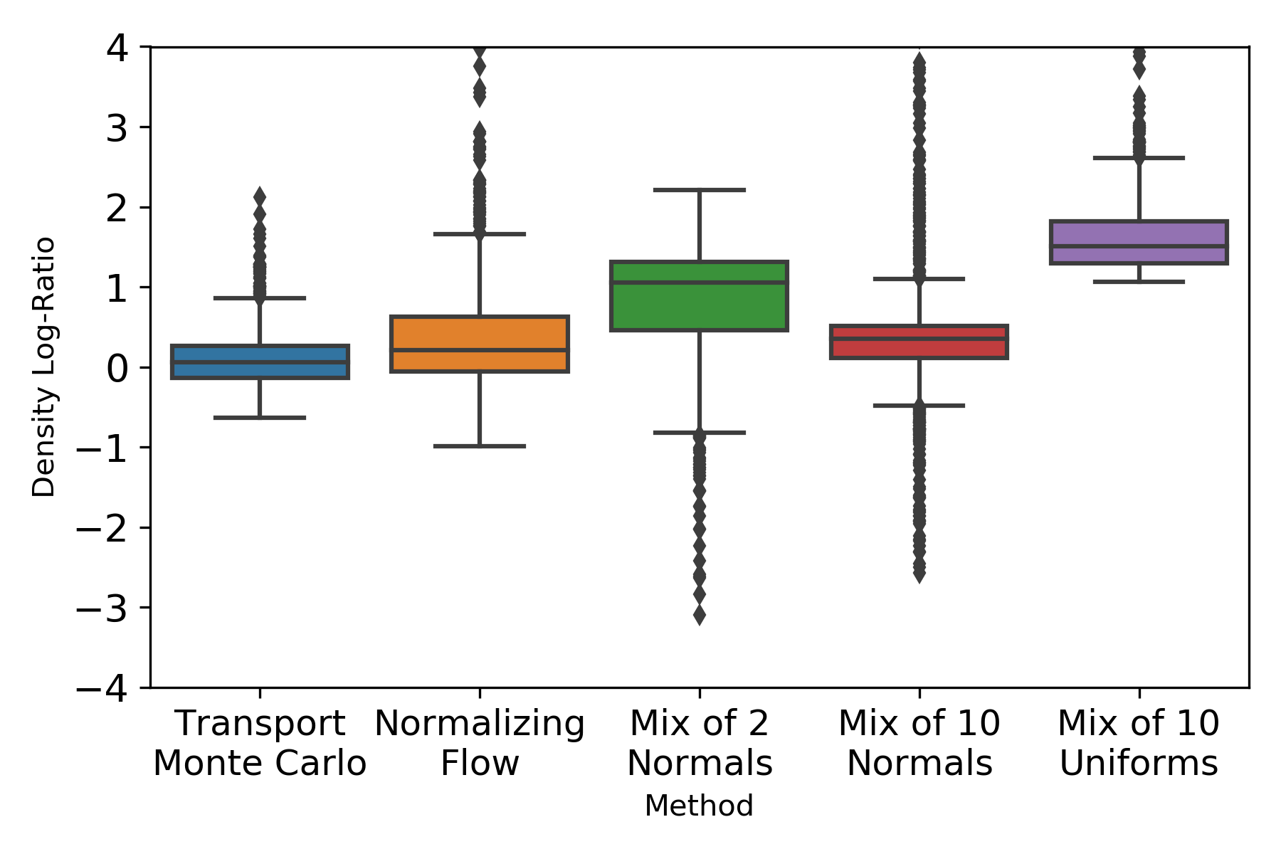
We first revisit the bivariate normal mixture example as in the main text. Since the target density $\Pi(\theta)$ is fully known including the normalizing constant $z(y)$ , we can compute $\log\{\tilde{\Pi}(\theta)/\Pi(\theta;y)\}$ directly and compare the mean log-ratio (empirical KL divergence) against the ideal $\mathbb{E}_{\theta\sim\tilde{\Pi}(\theta)}\log\{\tilde{\Pi}(\theta)/\Pi(\theta;y)\}=0$ .

Figure 7(a) plots the the log-density ratio $\log\{\tilde{\Pi}(\theta)/\Pi(\theta;y)\}$ based on the samples collected using various method. The TMC (panel b) showed very high accuracy, with the mean log-ratio $0.10$ . The deterministic transport using normalizing flow (panel c) also showed high accuracy (mean log-ratio $0.22$ ), although it used a large number of working parameters in the transform (total $804,900$ , versus $80$ used in the TMC). On the other hand, for the variational approximations, due to the diagonal covariance, the one using a 2-component normal mixture (panel d) gave a poor result (mean log-ratio $0.78$ ); and increasing the number of components to $10$ (panel e) reduced it to $0.60$ . The simple mixture of 10-component uniforms had the worst result (panel f) with the mean log-ratio $1.97$ — clearly, the dramatic difference between the simple uniform mixture and the TMC was due to the varying mixture weight $v_{k}(\beta)$ in the latter.

We next sample from a more challenging density that contains multiple local maxima:

	$\displaystyle\Pi(\theta;y)=$	$\displaystyle z(\lambda)^{-1}\exp\{\lambda H(\theta_{1},\theta_{2})\},$
	$\displaystyle H(\theta_{1},\theta_{2})=$	$\displaystyle\{\theta_{1}\sin(20\theta_{2})+y\sin(20\theta_{1})\}^{2}\cosh\{\sin(10\theta_{1})\theta_{1}\}\$
		$\displaystyle+\{\theta_{1}\cos(10\theta_{2})-\theta_{2}\sin(10\theta_{1})\}^{2}\cosh\{\cos(20\theta_{2})\theta_{2}\}.$

with support in $(-1.1,1.1)^{2}$ .

This example was originally proposed by Robert and Casella 2013 and later modified by Liang 2005. We plot the $H(\theta_{1},\theta_{2})$ function in Figure 8(a). And we chose $\lambda=1.2$ , so that the high probability region is dominated by $8$ major peaks, located near the four corners of the support. Using numerical integration, we have the normalizing constant $z(\lambda)\approx 173.1$ . We used $K=100$ in the TMC and $100$ components in all the mixture-based methods.

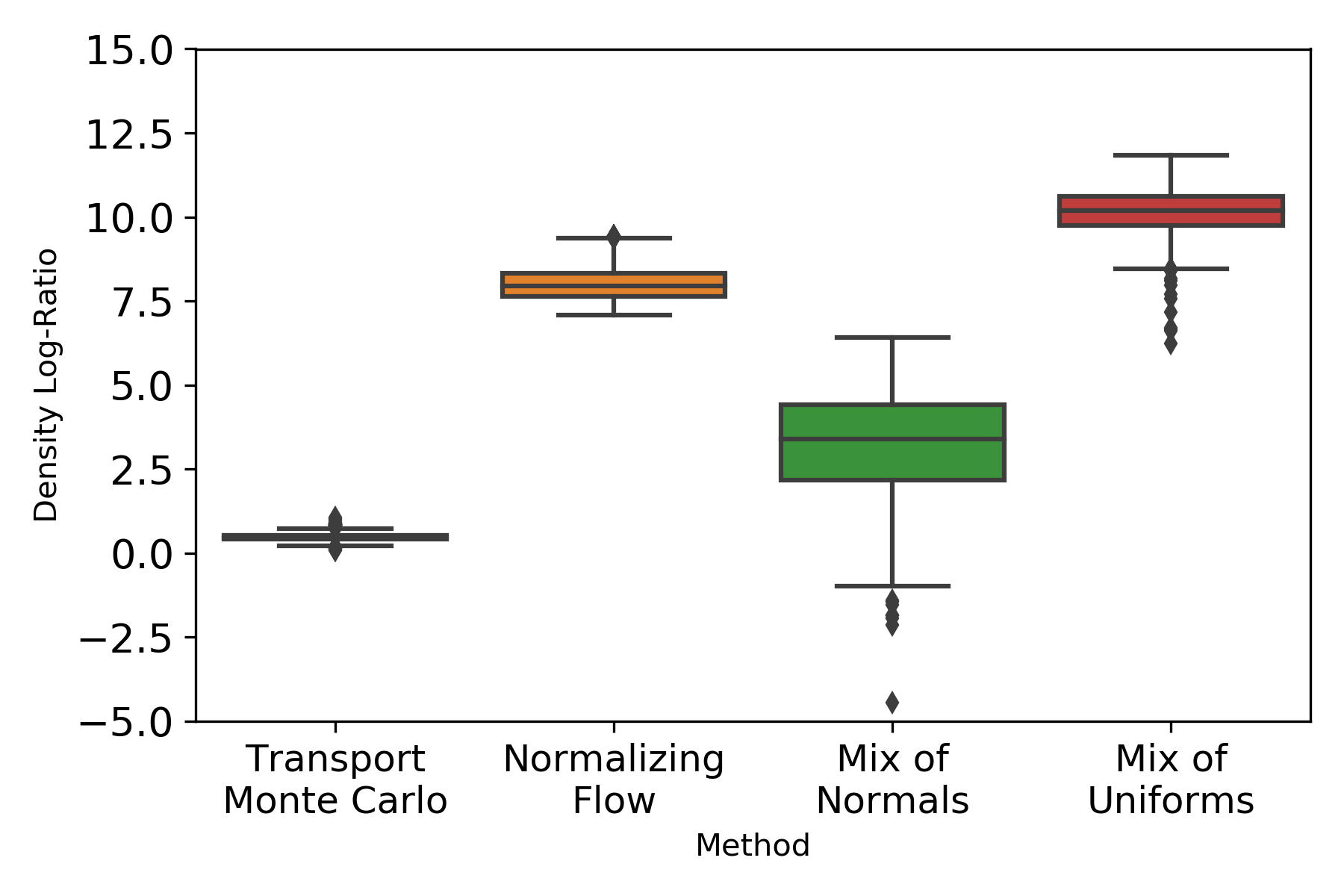
Figure 8(b) shows the log-density ratios. The Transport Monte Carlo showed a very low approximation error with the mean log-ratio $0.47$ , and the generated samples indeed recovered the $8$ density peaks (panel c). On the other hand, since the target distribution was no longer normal, the variational inference with normal mixture performed much worse this time, with the mean log-ratio $3.18$ ; the one with the uniform mixture had a mean log-ratio $10.01$ . The normalizing flow neural network had a surprisingly poor mean log-ratio $8.00$ , despite the large number of working parameters it used — we found out that all of the produced samples were trapped near one local density maximum.

In both the simulated examples above, it is worth noting that TMC also had the smallest standard deviation in the log-ratios. This can be particularly advantageous if we use the generated samples in the independence Hastings algorithm. In our experiments, The acceptance rates were $87\%$ in the first and $93\%$ in the second example.

Comparison with Normalizing Flow Neural Networks

As discussed in the introduction, the normalizing flow neural networks are a popular class of transport-based methods. They have demonstrated very good empirical performance, especially when the target density is log-concave.

On the other hand, the normalizing flow is known to have difficulties in handling a density with multiple local maxima. To demonstrate this, we experiment with a case of sampling from a $25$ -modal distribution:

\theta\sim\sum_{l=1}^{25}1/25\;\text{N}(\tilde{\mu}_{l},0.1^{2}),

where $\tilde{\mu}_{l}$ is from a two dimensional lattice ranging from $(-2,2)$ to $(2,2)$ . We used a small variance $0.1^{2}$ , so that the modes were well separated.

As shown, using the RealNVP normalizing flow (Dinh et al. 2017) (with $5$ layers, each with $256$ hidden units) resulted in a severe underestimation of the modes. Empirically, we found almost no difference when doubling the depth and/or width. We also experimented with other normalizing flow neural networks (Kingma et al. 2016; Papamakarios et al. 2017; Kingma and Dhariwal 2018). Although they improved the performance; however, none of them recovered all 25 modes.

In comparison, due to the use of multiple maps, the TMC is much less sensitive to this issue, and discovered all the modes in this case. As an alternative, one could use the normalizing flow as the mixture component transform in the TMC framework. We could not experiment with this extension, since each normalizing flow involved about $800,000$ to $1,200,000$ working parameters, which exceeded our memory capacity at $K\geq 3$ . Although at the larger computing system, we can expect to see an improved performance.

Example of Diagnostic Plot on $K$

References

Ambrosio et al. (2008) Ambrosio, L., N. Gigli, and G. Savaré (2008). Gradient Flows: In Metric Spaces and in the Space of Probability Measures. Springer Science & Business Media.
Beaumont et al. (2009) Beaumont, M. A., J.-M. Cornuet, J.-M. Marin, and C. P. Robert (2009). Adaptive Approximate Bayesian Computation. Biometrika 96(4), 983–990.
Bhadra et al. (2019) Bhadra, A., J. Datta, N. G. Polson, and B. Willard (2019). Lasso Meets Horseshoe: A Survey. Statistical Science 34(3), 405–427.
Bhattacharya et al. (2016) Bhattacharya, A., A. Chakraborty, and B. K. Mallick (2016). Fast Sampling With Gaussian Scale Mixture Priors in High-Dimensional Regression. Biometrika, 985–991.
Bhattacharya et al. (2015) Bhattacharya, A., D. Pati, N. S. Pillai, and D. B. Dunson (2015). Dirichlet–Laplace Priors for Optimal Shrinkage. Journal of the American Statistical Association 110(512), 1479–1490.
Bierkens et al. (2019) Bierkens, J., P. Fearnhead, and G. Roberts (2019). The Zig-Zag Process and Super-efficient Sampling for Bayesian Analysis of Big Data. Annals of Statistics 47(3), 1288–1320.
Bissiri et al. (2016) Bissiri, P. G., C. C. Holmes, and S. G. Walker (2016). A General Framework for Updating Belief Distributions. Journal of the Royal Statistical Society: Series B (Statistical Methodology) 78(5), 1103–1130.
Blei et al. (2017) Blei, D. M., A. Kucukelbir, and J. D. McAuliffe (2017). Variational Inference: a Review for Statisticians. Journal of the American Statistical Association 112(518), 859–877.
Carvalho et al. (2010) Carvalho, C. M., N. G. Polson, and J. G. Scott (2010). The Horseshoe Estimator for Sparse Signals. Biometrika 97(2), 465–480.
Castillo et al. (2015) Castillo, I., J. Schmidt-Hieber, and A. Van der Vaart (2015). Bayesian Linear Regression with Sparse Priors. The Annals of Statistics 43(5), 1986–2018.
Chen et al. (2018) Chen, R. T., Y. Rubanova, J. Bettencourt, and D. Duvenaud (2018). Neural Ordinary Differential Equations. In Advances in Neural Information Processing Systems, pp. 261–272. Curran Associates, Inc.
Cobb et al. (2019) Cobb, A. D., A. G. Baydin, A. Markham, and S. J. Roberts (2019). Introducing an Explicit Symplectic Integration Scheme for Riemannian Manifold Hamiltonian Monte Carlo. arXiv preprint arXiv:1910.06243.
Cobb and Jalaian (2020) Cobb, A. D. and B. Jalaian (2020). Scaling Hamiltonian Monte Carlo Inference for Bayesian Neural Networks With Symmetric Splitting. arXiv preprint arXiv:2010.06772.
Cuturi (2013) Cuturi, M. (2013). Sinkhorn Distances: Lightspeed Computation of Optimal Transport. Advances in Neural Information Processing Systems 26, 2292–2300.
Deheuvels et al. (1986) Deheuvels, P. et al. (1986). On the Influence of the Extremes of an IID Sequence on the Maximal Spacings. The Annals of Probability 14(1), 194–208.
Devroye (1982) Devroye, L. (1982). A Log Log Law for Maximal Uniform Spacings. Annals of Probability 10(3), 863–868.
Dinh et al. (2017) Dinh, L., J. Sohl-Dickstein, and S. Bengio (2017). Density Estimation using Real NVP. In International Conference on Learning Representations.
Doucet et al. (2021) Doucet, A., J. Heng, and Y. Pokern (2021). Gibbs Flow for Approximate Transport With Applications to Bayesian Computation. Journal of the Royal Statistical Society: Series B (Statistical Methodology), (in press).
Duan et al. (2018) Duan, L. L., J. E. Johndrow, and D. B. Dunson (2018). Scaling Up Data Augmentation MCMC via Calibration. The Journal of Machine Learning Research 19(1), 2575–2608.
Dunson et al. (2007) Dunson, D. B., N. Pillai, and J.-H. Park (2007). Bayesian Density Regression. Journal of the Royal Statistical Society: Series B (Statistical Methodology) 69(2), 163–183.
El Moselhy and Marzouk (2012) El Moselhy, T. A. and Y. M. Marzouk (2012). Bayesian Inference with Optimal Maps. Journal of Computational Physics 231(23), 7815–7850.
Fearnhead et al. (2018) Fearnhead, P., J. Bierkens, M. Pollock, and G. O. Roberts (2018). Piecewise Deterministic Markov Processes for Continuous-time Monte Carlo. Statistical Science 33(3), 386–412.
Giordano et al. (2018) Giordano, R., T. Broderick, and M. I. Jordan (2018). Covariances, Robustness and Variational Bayes. Journal of Machine Learning Research 19(1), 1981–2029.
Girolami and Calderhead (2011) Girolami, M. and B. Calderhead (2011). Riemann Manifold Langevin and Hamiltonian Monte Carlo Methods. Journal of the Royal Statistical Society: Series B (Statistical Methodology) 73(2), 123–214.
Ishwaran and Zarepour (2002) Ishwaran, H. and M. Zarepour (2002). Exact and Approximate Sum Representations for the Dirichlet Process. Canadian Journal of Statistics 30(2), 269–283.
Johndrow et al. (2019) Johndrow, J. E., A. Smith, N. Pillai, and D. B. Dunson (2019). MCMC for Imbalanced Categorical Data. Journal of the American Statistical Association 114(527), 1394–1403.
Kantorovich (1942) Kantorovich, L. V. (1942). On the Translocation of Masses. In Dokl. Akad. Nauk. USSR (NS), Volume 37, pp. 199–201.
Kingma and Ba (2014) Kingma, D. P. and J. Ba (2014). ADAM: a Method for Stochastic Optimization. In International Conference on Learning Representations.
Kingma and Dhariwal (2018) Kingma, D. P. and P. Dhariwal (2018). Glow: Generative Flow with Invertible 1x1 Convolutions. In Advances in Neural Information Processing Systems, pp. 10215–10224.
Kingma et al. (2016) Kingma, D. P., T. Salimans, R. Jozefowicz, X. Chen, I. Sutskever, and M. Welling (2016). Improved Variational Inference with Inverse Autoregressive Flow. In Advances in Neural Information Processing Systems, pp. 4743–4751.
Kingma and Welling (2014) Kingma, D. P. and M. Welling (2014). Auto-Encoding Variational Bayes. In International Conference on Learning Representations.
Kolouri et al. (2019) Kolouri, S., K. Nadjahi, U. Simsekli, R. Badeau, and G. Rohde (2019). Generalized Sliced Wasserstein Distances. In H. Wallach, H. Larochelle, A. Beygelzimer, F. d'Alché-Buc, E. Fox, and R. Garnett (Eds.), Advances in Neural Information Processing Systems, Volume 32, pp. 261–272. Curran Associates, Inc.
Kong and Chaudhuri (2020) Kong, Z. and K. Chaudhuri (2020). The Expressive Power of a Class of Normalizing Flow Models. In International Conference on Artificial Intelligence and Statistics, Volume 108, pp. 3599–3609.
Liang (2005) Liang, F. (2005). A Generalized Wang–Landau Algorithm for Monte Carlo Computation. Journal of the American Statistical Association 100(472), 1311–1327.
Mengersen and Tweedie (1996) Mengersen, K. L. and R. L. Tweedie (1996). Rates of Convergence of the Hastings and Metropolis Algorithms. Annals of Statistics 24(1), 101–121.
Miller et al. (2017) Miller, A. C., N. J. Foti, and R. P. Adams (2017). Variational Boosting: Iteratively Refining Posterior Approximations. In International Conference on Machine Learning, pp. 2420–2429. PMLR.
Monge (1781) Monge, G. (1781). Mémoire sur la théorie des déblais et des remblais. Histoire de l’Académie Royale des Sciences de Paris.
Neal (2011) Neal, R. M. (2011). MCMC using Hamiltonian Dynamics. Handbook of Markov Chain Monte Carlo 2(11), 2.
Nishimura et al. (2020) Nishimura, A., D. B. Dunson, and J. Lu (2020). Discontinuous Hamiltonian Monte Carlo for Discrete Parameters and Discontinuous Likelihoods. Biometrika 107(2), 365–380.
Pakman and Paninski (2013) Pakman, A. and L. Paninski (2013). Auxiliary-variable Exact Hamiltonian Monte Carlo Samplers for Binary Distributions. In C. J. C. Burges, L. Bottou, M. Welling, Z. Ghahramani, and K. Q. Weinberger (Eds.), Advances in Neural Information Processing Systems, Volume 26, pp. 2490–2498. Curran Associates, Inc.
Papamakarios et al. (2017) Papamakarios, G., T. Pavlakou, and I. Murray (2017). Masked Autoregressive Flow for Density Estimation. In Advances in Neural Information Processing Systems, pp. 2338–2347.
Parno and Marzouk (2018) Parno, M. D. and Y. M. Marzouk (2018). Transport Map Accelerated Markov Chain Monte Carlo. SIAM/ASA Journal on Uncertainty Quantification 6(2), 645–682.
Piironen and Vehtari (2017) Piironen, J. and A. Vehtari (2017). Sparsity Information and Regularization in the Horseshoe and Other Shrinkage Priors. Electronic Journal of Statistics 11(2), 5018–5051.
Rajaratnam and Sparks (2015) Rajaratnam, B. and D. Sparks (2015). MCMC-based Inference in the Era of Big Data: A Fundamental Analysis of the Convergence Complexity of High-Dimensional Chains. arXiv preprint arXiv:1508.00947.
Rezende and Mohamed (2015) Rezende, D. and S. Mohamed (2015, 07–09 Jul). Variational Inference with Normalizing Flows. In Proceedings of the 32nd International Conference on Machine Learning, Volume 37, pp. 1530–1538.
Robert and Casella (2013) Robert, C. and G. Casella (2013). Monte Carlo Statistical Methods. Springer Science & Business Media.
Robert et al. (2018) Robert, C. P., V. Elvira, N. Tawn, and C. Wu (2018). Accelerating MCMC Algorithms. Wiley Interdisciplinary Reviews: Computational Statistics 10(5), e1435.
Roberts and Tweedie (1996) Roberts, G. O. and R. L. Tweedie (1996). Exponential Convergence of Langevin Distributions and Their Discrete Approximations. Bernoulli 2(4), 341–363.
Schilling (2017) Schilling, R. L. (2017). Measures, Integrals and Martingales. Cambridge University Press.
Sojoudi (2016) Sojoudi, S. (2016). Equivalence of Graphical Lasso and Thresholding for Sparse Graphs. Journal of Machine Learning Research 17(1), 3943–3963.
Solomon et al. (2015) Solomon, J., F. De Goes, G. Peyré, M. Cuturi, A. Butscher, A. Nguyen, T. Du, and L. Guibas (2015). Convolutional Wasserstein Distances: Efficient Optimal Transportation on Geometric Domains. ACM Transactions on Graphics 34(4), 1–11.
Spantini et al. (2018) Spantini, A., D. Bigoni, and Y. Marzouk (2018). Inference via Low-Dimensional Couplings. The Journal of Machine Learning Research 19(1), 2639–2709.
Tierney (1994) Tierney, L. (1994). Markov Chains for Exploring Posterior Distributions. The Annals of Statistics, 1701–1728.

		$\displaystyle\frac{\cancel{\Pi(\theta^{};y)}\tilde{\Pi}(\beta^{}\mid\theta^{})}{\cancel{\Pi(\theta^{t};y)}\tilde{\Pi}(\beta^{t}\mid\theta^{t})}\frac{\{\rho\Pi_{r}(\beta^{t})+(1-\rho)\Pi_{a}(\beta^{t})\}\frac{w_{c^{t}}\{T_{c^{t}}(\beta^{t})\}\cancel{\Pi\{T_{c^{t}}(\beta^{t});y\}}{{\|\textup{det}\nabla T_{c^{t}}(\beta^{t})\|}}1\{\theta^{t}=T_{c^{t}}(\beta^{t}),T_{c^{t}}(\beta^{t})\in\Theta\}}{\sum_{k=1}^{\infty}w_{k}\{T_{k}(\beta^{t})\}\Pi\{T_{k}(\beta^{t});y\}{\|\textup{det}\nabla T_{k}(\beta^{t})\|1\{T_{k}(\beta^{t})\in\Theta\}}}}{\{\rho\Pi_{r}(\beta^{})+(1-\rho)\Pi_{a}(\beta^{})\}\frac{w_{c^{}}\{T_{c^{}}(\beta^{})\}\cancel{\Pi\{T_{c^{}}(\beta^{});y\}}{{\|\textup{det}\nabla T_{c^{}}(\beta^{})\|}}1\{\theta^{}=T_{c^{}}(\beta^{}),T_{c^{}}(\beta^{})\in\Theta\}}{\sum_{k=1}^{\infty}w_{k}\{T_{k}(\beta^{})\}\Pi\{T_{k}(\beta^{});y\}{\|\textup{det}\nabla T_{k}(\beta^{})\|1\{T_{c^{}}(\beta^{})\in\Theta\}}}}$
		$\displaystyle=\frac{\cancel{\tilde{\Pi}(\beta^{}\mid\theta^{})}}{\cancel{\tilde{\Pi}(\beta^{t}\mid\theta^{t})}}\frac{\{\rho\Pi_{r}(\beta^{t})+(1-\rho)\Pi_{a}(\beta^{t})\}\frac{\cancel{w_{c^{t}}\{T_{c^{t}}(\beta^{t})\}}{{\|\textup{det}\nabla T_{c^{t}}(\beta^{t})\|}}1\{\theta^{t}=T_{c^{t}}(\beta^{t})\}}{\sum_{k=1}^{\infty}w_{k}\{T_{k}(\beta^{t})\}\Pi\{T_{k}(\beta^{t});y\}{\|\textup{det}\nabla T_{k}(\beta^{t})\|1\{T_{k}(\beta^{t})\in\Theta\}}}}{\{\rho\Pi_{r}(\beta^{})+(1-\rho)\Pi_{a}(\beta^{})\}\frac{\cancel{w_{c^{}}\{T_{c^{}}(\beta^{})\}}{{\|\textup{det}\nabla T_{c^{}}(\beta^{})\|}}1\{\theta^{}=T_{c^{}}(\beta^{})\}}{\sum_{k=1}^{\infty}w_{k}\{T_{k}(\beta^{})\}\Pi\{T_{k}(\beta^{});y\}{\|\textup{det}\nabla T_{k}(\beta^{})\|1\{T_{c^{}}(\beta^{*})\in\Theta\}}}}$
		$\displaystyle=\frac{\{\rho\Pi_{r}(\beta^{t})+(1-\rho)\Pi_{a}(\beta^{t})\}\|\textup{det}\nabla T_{c^{t}}(\beta^{t})\|{\sum_{k=1}^{\infty}w_{k}\{T_{k}(\beta^{})\}\Pi\{T_{k}(\beta^{});y\}{\|\textup{det}\nabla T_{k}(\beta^{})\|1\{T_{c^{}}(\beta^{})\in\Theta\}}}}{\{\rho\Pi_{r}(\beta^{})+(1-\rho)\Pi_{a}(\beta^{})\}\|\textup{det}\nabla T_{c^{}}(\beta^{*})\|{\sum_{k=1}^{\infty}w_{k}\{T_{k}(\beta^{t})\}\Pi\{T_{k}(\beta^{t});y\}{\|\textup{det}\nabla T_{k}(\beta^{t})\|1\{T_{c^{t}}(\beta^{t})\in\Theta\}}}}$
		$\displaystyle=\frac{\{\rho\Pi_{r}(\beta^{t})+(1-\rho)\Pi_{a}(\beta^{t})\}\|\textup{det}\nabla T_{c^{t}}(\beta^{t})\|\tilde{\Pi}(\beta^{})}{\{\rho\Pi_{r}(\beta^{})+(1-\rho)\Pi_{a}(\beta^{})\}\|\textup{det}\nabla T_{c^{}}(\beta^{*})\|\tilde{\Pi}(\beta^{t})}.$

	$\displaystyle\|\int_{\mathcal{A}}\int_{\Theta}$	$\displaystyle\{\tilde{\Pi}(\beta\mid\theta)-\Pi(\beta\mid\theta)\}\Pi(\theta;y)\textup{d}\theta\textup{d}\beta\|$
		$\displaystyle\stackrel{{\scriptstyle(i)}}{{=}}\|\int_{\Theta}\int_{\mathcal{A}}\{\tilde{\Pi}(\beta\mid\theta)-\Pi(\beta\mid\theta)\}\textup{d}\beta\Pi(\theta;y)\textup{d}\theta\|$
		$\displaystyle\stackrel{{\scriptstyle(ii)}}{{\leq}}\|\int_{\Theta^{}}\int_{\mathcal{A}}\{\tilde{\Pi}(\beta\mid\theta)-\Pi(\beta\mid\theta)\}\textup{d}\beta\Pi(\theta;y)\textup{d}\theta\|+\|\int_{\Theta\setminus\Theta^{}}\int_{\mathcal{A}}\{\tilde{\Pi}(\beta\mid\theta)-\Pi(\beta\mid\theta)\}\textup{d}\beta\Pi(\theta;y)\textup{d}\theta\|$
		$\displaystyle\leq\epsilon/2\int_{\Theta^{}}\Pi(\theta;y)\textup{d}\theta+\|\int_{\Theta\setminus\Theta^{}}1\;\Pi(\theta;y)\textup{d}\theta\|$
		$\displaystyle\stackrel{{\scriptstyle(iii)}}{{\leq}}\epsilon/2+\epsilon/2$
		$\displaystyle=\epsilon$

	$\displaystyle\bigg\|\frac{\partial g(\beta)}{\partial\beta_{\{j\}}}\bigg\|=$	$\displaystyle\bigg\|\sum_{k=1}^{K}\frac{\exp h_{k}(\beta)\partial h_{k}(\beta)/\partial\beta_{\{j\}}}{\sum_{l=1}^{K}\exp h_{l}(\beta)}\bigg\|$
	$\displaystyle\leq$	$\displaystyle\sum_{k=1}^{K}\frac{\exp h_{k}(\beta)}{\sum_{l=1}^{K}\exp h_{l}(\beta)}\bigg\|\frac{\partial h_{k}(\beta)}{\partial\beta_{\{j\}}}\bigg\|$
	$\displaystyle\leq$	$\displaystyle\max_{k\in\{1\ldots K\}}\bigg\|\frac{\partial h_{k}(\beta)}{\partial\beta_{\{j\}}}\bigg\|.$

Transport Monte Carlo: High-Accuracy Posterior Approximation via Random Transport

1 Introduction

2 Transport Monte Carlo

2.1 Two Types of Transport: Deterministic versus Random

2.2 Random Transport Plan as an Infinite Mixture

Remark 1 (Difference from a mixture-based variational approximation).

Remark 2.

2.3 Parameterizing the Mixture Weight and Transform

2.4 Transport to Discrete Posterior

3 Transport Monte Carlo Algorithm

3.1 Algorithm

3.2 Details on the Optimization

3.2.1 Component-wise Optimization

3.2.2 Diagnostics on KK and Convergence

Remark 3.

3.2.3 Initialization

3.3 Combining with Independence Hastings Algorithm

4 Theoretic Study

Theorem 1.

Theorem 2.

Theorem 3.

Theorem 4.

5 Comparison with the Hamiltonian Monte Carlo

6 Application: Graph Estimation under Degree Regularization

7 Discussion

Acknowledgement

Extension: Independence Hastings Algorithm

Remark 4.

Details of Hastings Acceptance Rate

Table of an Approximate Transport Plan

Proof of Theorem 1

Proof of Theorem 2

Proof.

Proof of Theorem 3

Proof.

Proof of Theorem 4

Proof.

Simulation: High Dimensional Regression using the Shrinkage Prior

Benchmark: Assessing Approximation Error

Comparison with Normalizing Flow Neural Networks

Example of Diagnostic Plot on KK

References

Transport Monte Carlo:
High-Accuracy Posterior Approximation
via Random Transport

3.2.2 Diagnostics on $K$ and Convergence

Example of Diagnostic Plot on $K$