Squeezed state metrology with Bragg interferometers operating in a cavity

We consider a collection of $N$ atoms with mass $M$ in a ring cavity with resonance frequency $\omega_{c}$ as shown in Fig. 1(a). Each atom consists of two electronic levels $\ket{g}$ and $\ket{e}$ with transition frequency $\omega_{a}$. A laser with frequency $\omega_{l}$ drives one mode of the ring cavity. The cavity resonance is red detuned from the atomic transition by a detuning $\Delta_{c}=\omega_{a}-\omega_{c}>0$, while the drive laser is detuned by $\Delta_{l}=\omega_{a}-\omega_{l}>0$. The relative detuning of the laser and the cavity is $\Delta_{cl}=\omega_{l}-\omega_{c}\ll\Delta_{c},\Delta_{l}$. Upon absorption or emission of a photon with wavevector $\mathbf{k}$, the momentum of an atom is shifted by $\hbar k$, where $k=\lvert\mathbf{k}\rvert$.

We now proceed to derive a master equation that reflects the underlying atom-cavity interaction at the heart of the resonant spin exchange intuitively described in the previous section. The Hamiltonian governing the dynamics of the atom-cavity system is

where $g$ is the atom-cavity vacuum Rabi frequency, $\kappa$ is the cavity decay rate and $\alpha$ is the amplitude of the drive laser with $\lvert\alpha\rvert^{2}$ the photon flux in units of photons/time. The operators $\hat{a}^{\dagger}_{s},\hat{a}_{s}$ for $s=1,2$ respectively describe the creation and annihilation of photons in modes 1 and 2 whose wavevectors satisfy $\mathbf{k}_{1}=-\mathbf{k}_{2}=k\mathbf{\hat{z}}$ (see Fig. (1)(a)). The operator $\hat{z}_{j}$ represents the position of atom $j$ along the cavity axis. The decay of the cavity fields is accounted for by the standard Lindblad dissipator of the type $\mathcal{D}[\hat{O}]\rho=\hat{O}\rho\hat{O}^{\dagger}-\hat{O}^{\dagger}\hat{O}\rho/2-\rho\hat{O}^{\dagger}\hat{O}/2$ for jump operator $\hat{O}$ and density matrix $\rho$. The resulting master equation is

We neglect free-space scattering in our analysis since superradiant decay (Section (3.4)) is typically the dominant dissipation mechanism (see F and discussion in Section 4).

We work in an interaction picture rotating at the drive frequency $\omega_{l}$ with free evolution Hamiltonian $H_{f}=\sum_{j}\hbar\omega_{l}/2(\ket{e}_{j}\bra{e}-\ket{g}_{j}\bra{g})+\sum_{s}\omega_{l}\hat{a}_{s}^{\dagger}\hat{a}_{s}$. First, we adiabatically eliminate the excited state $\ket{e}$ based on the large detuning of the drive lasers and cavity modes from the $\ket{g}\leftrightarrow\ket{e}$ transition (A.1). Further, on long timescales, the upwards propagating mode (mode 1) is composed of a macroscopic steady state amplitude with small fluctuations around this value. The macroscopic amplitude $\beta$ ($\lvert\beta\rvert\gg 1$) is found from the mean-field equation

For $t\gg\kappa^{-1}$, the steady-state value is $\beta=-i\sqrt{\kappa}\alpha/(\kappa/2-i\Delta_{cl})$. We displace mode 1 by the amplitude $\beta$ by making the transformation $\hat{a}_{1}\rightarrow\beta+\hat{a}_{1}$. Apart from introducing some constant terms that can be neglected, the resulting Hamiltonian is

with $k_{\text{eff}}=k_{1}-k_{2}=2k$ the effective wavevector along $\mathbf{\hat{z}}$. The dissipative part of the master equation remains the same. The second line of Eq. (8) reflects the dominant photon exchange between the macroscopic field in mode 1 and the vacuum of mode 2. In writing Eq. (8), we have neglected the small exchange process between the vacuum fields of the two modes. This approximation allows us to keep track of only mode 2 and ignore the other terms containing $\hat{a}_{1}$ in the master equation since mode 1 only interacts with the atoms and mode 2 through the $c$-number $\beta$.

The master equation governing the atom-cavity interactions is:

We write down the dynamical equations for the corresponding $c$-numbers $s_{nm}^{j}\leftrightarrow\hat{\sigma}_{nm}^{j}$ and $\zeta\leftrightarrow\hat{a}_{2}$ within the truncated Wigner approximation (TWA) framework [24]. We introduce the effective coupling strength $g_{\text{eff}}=g^{2}\lvert\beta\rvert/2\Delta_{c}$ and without loss of generality assume that $\beta$ is real. These equations are

where $\xi_{l}(t)$ for $l=1,2$ are white-noise processes satisfying $\overline{\xi_{l}(t)}=0$ and $\overline{\xi_{l}(t)\xi_{l^{\prime}}(t^{\prime})}=\delta_{l,l^{\prime}}\delta(t-t^{\prime})$. The bar indicates averaging over several trajectories with different noise realizations (and initial conditions, see Section 2.4.1) . The equation for $\zeta$ is a stochastic differential equation because of the noise arising from coupling to modes outside the cavity [26]. We refer to this model as the multi-center model (MCM) because of its ability to track an arbitrary number of momentum centers.

The spin exchange dynamics anticipated in Section 2.2 is confirmed when mode 2 is adiabatically eliminated to obtain a master equation describing the effective atom-atom interactions. When mode 2 is negligibly excited, it can be considered as a reservoir in a vacuum state with density matrix $R_{0}=\ket{0}\bra{0}$. We use the superoperator formalism to adiabatically eliminate mode 2 [27]. The details of this derivation are presented in A.2. The resulting master equation can be compactly expressed in terms of operators analogous to collective angular momentum operators, which we introduce below.

To make computations tractable, we assume that the $n_{\downarrow},n_{\uparrow}$ centers form a closed two-level system while studying the collective spin dynamics using the master equation, Eq. (27). To this effect, we truncate the master equation, Eq. (27), as

where the truncated Hamiltonian is

We recall that the effective Hamiltonian, Eq. (31), with $\tilde{\sigma}_{q}=0$ is analogous to the standard spin exchange/one-axis twisting model studied for closed two-level systems coupled to a cavity [2, 21, 22, 28] (also compare with Eq. (3)), and provides a reference model against which complications arising from the nature of momentum states can be contrasted.

Exact solutions even for the truncated master equation, Eq. (30), are computationally intractable because of the exponential scaling of the Liouville space with atom number. We use an approximate method where we only keep track of expectation values of single atom and two atom operators, of the type $\langle\hat{\sigma}_{n_{a},n_{b}}^{1,q}\rangle$ and $\langle\hat{\sigma}_{n_{a},n_{b}}^{1,q}\hat{\sigma}_{n_{c},n_{d}}^{2,q^{\prime}}\rangle$, where the $n$ values can take either $n_{\downarrow}$ or $n_{\uparrow}$. Since we are ignoring the other momentum centers, we refer to this model as the two-center model (TCM). As in the MCM, the single atom and two atom expectation values are first initialized according to the state described by Eq. (21). Next, an instantaneous rotation transforms these quantities to correspond to a state that is an equal superposition of $n_{\downarrow},n_{\uparrow}$ (B.2). The identical initial conditions for each atom and the permutation symmetry of the master equation enable us to avoid separate indices for every atom in the system, with the number of atoms $N$ explicitly appearing in the equations for the quantities $\langle\hat{\sigma}_{n_{a},n_{b}}^{1,q}\rangle$ and $\langle\hat{\sigma}_{n_{a},n_{b}}^{1,q}\hat{\sigma}_{n_{c},n_{d}}^{2,q^{\prime}}\rangle$. The resulting equations of motion for these single atom and two atom expectation values are summarized in C.

The $\hat{\mathcal{J}}_{n_{\downarrow}}^{z}\hat{\mathcal{J}}_{n_{\downarrow}}^{z}$ term implicit in Eq. (31) (see Eq. (4)) can be exploited to prepare spin squeezed states. The figure of merit of a squeezed state, relevant for quantum metrology, is the Wineland squeezing parameter $\xi_{\text{R}}^{2}$ [2] defined as

The contrast $\mathcal{C}$ is given by

where $\mathbf{\hat{J}_{n_{\downarrow}}}=\hat{\mathcal{J}}_{n_{\downarrow}}^{x}\mathbf{\hat{x}}+\hat{\mathcal{J}}_{n_{\downarrow}}^{y}\mathbf{\hat{y}}+\hat{\mathcal{J}}_{n_{\downarrow}}^{z}\mathbf{\hat{z}}$. For a given state, $V_{\text{min}}$ is the variance in a spin component in the plane perpendicular to the mean spin direction (MSD), minimized over all axes in this plane. Mathematically,

First, we note that the single atom-cavity vacuum Rabi frequency can be expressed as $g=\sqrt{C\kappa\gamma}$, where $C$ is the cooperativity of the cavity and $\gamma$ is the inverse lifetime of the excited state. Our model imposes two constraints that limit $\lvert\beta\rvert$ to the range

where we have used $g=\sqrt{C\kappa\gamma}$. The lower bound $\lvert\beta\rvert\gg 1$ allows us to treat mode 1 as a classical field represented by the $c$-number $\beta$. The upper bound ensures that the excited state $\ket{e}$ is negligibly populated, i.e.

thereby ensuring that the adiabatic elimination of $\ket{e}$ is valid. We work with $\lvert\beta\rvert$ values such that $\lvert\beta\rvert\geq 100$ and the excited state population is $\leq 0.01$.

Although our scheme is applicable to a wide variety of atomic species, here we consider its efficiency when it is implemented on the $689$ nm ${}^{1}\text{S}_{0}-{}^{3}\text{P}_{1}$ transition of ${}^{88}\text{Sr}$. Our choice is motivated by the advantages of using ground-state ${}^{88}\text{Sr}$ in Bragg interferometers [15], such as its extremely small scattering cross-section, insensitivity to stray magnetic fields and ease of experimental manipulation, including accessing the parameter regimes required for our scheme. The inverse lifetime of the excited state is $\gamma/2\pi=7.6$ kHz while the single photon recoil frequency is $\omega_{r}/2\pi=4.74$ kHz. The spin-1/2 system is encoded in $\ket{\downarrow}\equiv\ket{{}^{1}\text{S}_{0},0\hbar k}$ and $\ket{\uparrow}\equiv\ket{{}^{1}\text{S}_{0},2\hbar k}$ implying that $n_{\downarrow}=0,n_{\uparrow}=1$. We consider $N=10^{3}$ atoms in a cavity with decay rate $\kappa/2\pi=100$ kHz, and with either of two cooperativities, $C=1$ ($C=10$). The single atom-cavity vacuum Rabi frequency $g=\sqrt{C\kappa\gamma}$ then takes the value $g/2\pi\approx 27.6$ kHz ($87.2$ kHz). We assume that the cavity resonance is detuned from the atomic transition such that $\Delta_{c}/2\pi=200$ MHz. We characterize the relative strength of the dissipative and dispersive interactions by the ratio $R$ defined as

Squeezing by one-axis twisting occurs when the dispersive interactions dominate, corresponding to the regime $R\ll 1$. We consider $R$ in the range $0.025-0.2$ in our study. Model-enforced constraints (see Eq. (35) and the discussion following it) restrict the photon number in mode 1, $\lvert\beta\rvert^{2}$, to the range $1\times 10^{4}-2\times 10^{6}$ ($1\times 10^{4}-2\times 10^{5}$). Experimentally, these constraints translate to varying the power $P$ in the drive laser in a range $10\;\text{nW}-150\;\mu\text{W}$ ($10\;\text{nW}-15\;\mu\text{W}$) (D). In standard one-axis twisting with closed two level systems, squeezing proceeds at a characteristic rate $Q=N\chi_{n_{\downarrow}}$ [21, 28, 2]. The permissible values of $\lvert\beta\rvert^{2}$ results in a squeezing rate $Q/2\pi$ in the range $5\;\text{Hz}-7.6\;\text{kHz}$ ($0.5\;\text{kHz}-76\;\text{kHz}$) (D). We only consider squeezing rates such that $Q/\delta_{n_{\downarrow}}\ll 1$ ($<1/50$ in all simulations), allowing for the adiabatic elimination of mode 2 in deriving the two-center model (see A.3). Even in this regime, while very slow rates are undesirable from a technical perspective, very fast squeezing with $Q\gtrsim\omega_{r}$ leads to coupling with momentum states outside the pseudospin manifold and degrades the squeezing, as we will demonstrate.

Finally, to account for the momentum width of the atomic cloud, we consider values $\tilde{\sigma}_{q}\leq 0.1$ to satisfy the requirement, Eq. (11), of our model. The dephasing rate $\mu_{d}=4\sqrt{2}\omega_{r}\tilde{\sigma}_{q}$ associates a characteristic timescale to the momentum width. Specifically, for a collection of atoms initialized in the same, equal superposition between the two centers $n_{\downarrow},n_{\uparrow}$ and undergoing free evolution, the contrast $\mathcal{C}$ decays as $\mathcal{C}(t)=e^{-\mu_{d}^{2}t^{2}}$. With $\tilde{\sigma}_{q}\leq 0.1$, the corresponding maximum rate is $\mu_{d}/2\pi=2.7\;\text{kHz}$.

We first consider the case of $\tilde{\sigma}_{q}\approx 0$, i.e. negligible momentum width. Figure 2(a) plots the evolution of the spin squeezing parameter in the $C=1$ case for values of $R$ in the range $0.025-0.2$, and with $\lvert\beta\rvert^{2}\approx 5.4\times 10^{5}$. Modest laser powers, up to $40\;\mu$W, are sufficient to maintain this intracavity photon number for the range of $R$ considered here (D). In this parameter regime, the TCM (dashed) and MCM (solid) results agree excellently until $\xi_{\text{R}}^{2}$ reaches its minimum value. The minimum value of $\xi_{\text{R}}^{2}$ arises as a trade-off between the twisting dynamics that decreases $V_{\text{min}}$ (Eq. (32) and fluctuations in superradiant decay from $n_{\downarrow}$ to $n_{\uparrow}$ that increase this quantity [21, 28]. For smaller $R$, the larger value of $\delta_{n_{\downarrow}}$ strongly suppresses dissipation relative to dispersive interactions (Eq. (29)), leading to improved squeezing, i.e. smaller values of $\xi_{\text{R}}^{2}$. However, for fixed $\lvert\beta\rvert^{2}$, the absolute squeezing rate $N\chi_{n_{\downarrow}}$ also decreases with larger $\delta_{n_{\downarrow}}$ (Eq. (29)), leading to slower squeezing dynamics. Therefore, as summarized in the inset, smaller $R$ values enable greater metrological gain, but the time taken for squeezing also increases when $\lvert\beta\rvert^{2}$ is fixed.

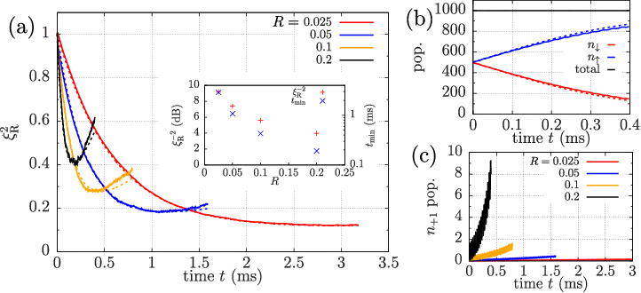
The population dynamics at the different momentum centers reveal the effect of superradiance. Figure 2(b) shows the evolution of populations in $n_{\downarrow},n_{\uparrow}$ for the case of $R=0.2$. The rapid decrease (increase) in $n_{\downarrow}$ ($n_{\uparrow}$) population reflects superradiant decay on the $n_{\downarrow}\rightarrow n_{\uparrow}$ transition. Further, the MCM enables an investigation of the leakage to centers outside the spin manifold, highlighting the power of this technique. We denote the first $k$ centers higher than $n_{\uparrow}$ as $n_{+k}$, and the first $k$ centers lower than $n_{\downarrow}$ as $n_{-k}$. The MCM reveals that a small number of atoms ($<10$) are lost to $n_{+1}$ during the squeezing dynamics, as seen in Fig. 2(c) for the various $R$ values. However, the excellent agreement between the TCM and MCM results in Fig. 2(a) indicates that in this parameter regime, the centers $n_{\downarrow},n_{\uparrow}$ can be effectively treated as a closed two-level spin-$1/2$ manifold.

A simple two-level model, such as the TCM, would predict that the squeezing rate can be arbitrarily increased by simply pumping in more laser power so that $\lvert\beta\rvert^{2}$ is increased. Figure 3(a) explores the evolution of $\xi_{\text{R}}^{2}$ in the case $C=10$, $R=0.05$ ($\delta_{n_{\downarrow}}/2\pi=1$ MHz) for different values of $\lvert\beta\rvert^{2}/10^{4}$ in the range $2-16$. As expected, the TCM (dashed) predicts that $\xi_{\text{R}}^{2}$ attains the same minimum value faster when $\lvert\beta\rvert^{2}$ is increased. However, the MCM results (solid) present a different narrative: As $\lvert\beta\rvert^{2}$ increases, $\xi_{\text{R}}^{2}$ indeed attains its minimum faster, but this value also increases, signaling a degradation of squeezing. In fact, the metrological gain $\xi_{\text{R}}^{-2}$ drops by $\sim 3$ dB (factor of 2) as $\lvert\beta\rvert^{2}$ increases from $2\times 10^{4}$ to $16\times 10^{4}$.

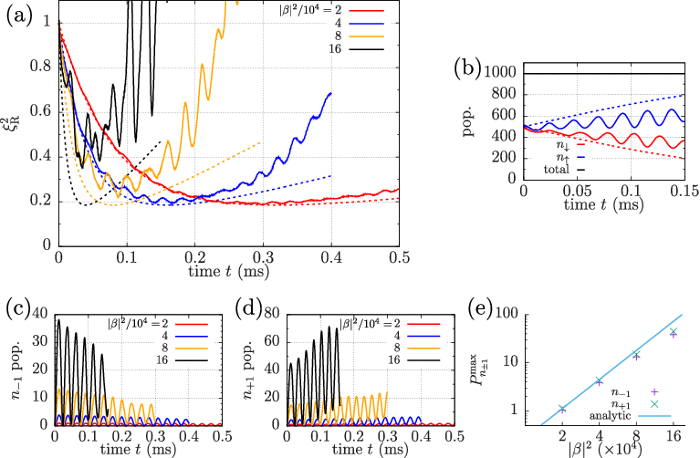
Large oscillations in the MCM curves as $\lvert\beta\rvert^{2}$ is increased indicates the breakdown of the two-state model. A study of the population dynamics at the different centers confirms this breakdown. As seen in Fig. 3(b), although the populations in $n_{\downarrow}$ ($n_{\uparrow}$) follow the general decreasing (increasing) trend expected from $n_{\downarrow}\rightarrow n_{\uparrow}$ superradiant decay, the TCM and MCM population transients significantly differ in the case of strong driving ($\lvert\beta\rvert^{2}/10^{4}=16$). Further, the MCM transients display pronounced oscillations with a frequency $\sim 8\omega_{r}$, corresponding to the relative detuning between the $n_{\downarrow}\leftrightarrow n_{\uparrow}$ and $n_{\uparrow}\leftrightarrow n_{+1}$, $n_{-1}\leftrightarrow n_{\downarrow}$ transitions.

Giant population oscillations in $n_{\pm 1}$, shown in Fig. 3(c-d), confirm the significant participation of these centers in the dynamics as $\lvert\beta\rvert^{2}$ increases. A simple Rabi oscillation model qualitatively explains the occupation of these states: The coherent superposition of the $n_{\downarrow},n_{\uparrow}$ centers serves as a large collective spin that sources mode 2. Both cavity modes, 1 and 2, are now macroscopically occupied and drive two-photon Rabi oscillations between $n_{\downarrow}\leftrightarrow n_{-1}$ and $n_{\uparrow}\leftrightarrow n_{+1}$ with approximate two-photon detuning $8\omega_{r}$. We find that the maximum population $P_{n_{\pm 1}}^{\text{max}}$ in $n_{\pm 1}$ predicted by this model is given by (see E)

Figure 3(e) compares the first oscillation peak in the $n_{\pm 1}$ populations with the analytic formula Eq. (38). For small occupations (small $\lvert\beta\rvert^{2}$), the formula agrees very well with the simulations, whereas the discrepancy becomes about a factor of 2 at the largest occupation ($\lvert\beta\rvert^{2}=16\times 10^{4}$). In this strong driving regime, the coherence that develops between $n_{\uparrow},n_{+1}$ and $n_{\downarrow},n_{-1}$ is no longer negligible and modifies the field in mode 2 considerably, leading to the breakdown of the simple Rabi oscillation picture presented here (E).

We also note that the amplitude of population oscillations in $n_{-1}$ ($n_{+1}$) decreases (increases) over time, as evident in Fig. 3(c) (Fig. 3(d)). The reason is that $n_{\downarrow}\rightarrow n_{\uparrow}$ superradiant decay irreversibly removes (introduces) atoms participating in the $n_{\downarrow}\leftrightarrow n_{-1}$ ($n_{\uparrow}\leftrightarrow n_{+1}$) Rabi cycles. Finally, the troughs, and consequently the peaks, of the oscillations in $n_{+1}$ population are clearly seen to rise with time because of the direct cavity mediated decay on the $n_{\uparrow}\rightarrow n_{+1}$ transitions superposed on the Rabi oscillations. Similarly, the interplay of Rabi oscillations and cavity mediated decay on the $n_{-1}\rightarrow n_{\downarrow}$ transition causes the troughs in the $n_{-1}$ oscillations to deviate from zero over time.

We now consider the case when the atomic cloud has non-zero momentum width. For this study, we use the parameters from Fig. 3, i.e. $C=10$ and $\lvert\beta\rvert^{2}/10^{4}=2,4,8,16$. Fig. 4(a) shows the evolution of $\xi_{\text{R}}^{2}$ for $\tilde{\sigma}_{q}=0,0.025,0.05$ and $0.1$ in the case when $\lvert\beta\rvert^{2}/10^{4}=4$. In this panel, the solid and dashed curves respectively indicate the MCM and TCM models. Three trends can be observed from this figure: (T1) When the rate of squeezing is fast relative to the dephasing ($\propto\tilde{\sigma}_{q}$), the $\xi_{\text{R}}^{2}$ transient is similar (blue) to the zero width case (red) while the minimum value attained is greater indicating slight degradation of squeezing. (T2) For larger momentum width, the $\xi_{\text{R}}^{2}$ transient displays oscillatory behavior signifying competition between squeezing and dephasing (orange). (T3) As the width increases further and dephasing dominates, $\xi_{\text{R}}^{2}$ initially decreases slightly but then steeply increases to values well above unity, signaling rapid loss of squeezing (black).

These trends are summarized in Fig. 4(b), where the maximum metrological gain achievable is plotted as a function of $\lvert\beta\rvert^{2}$ for different values of $\tilde{\sigma}_{q}$. The $\tilde{\sigma}_{q}=0$ case (red) reflects the study performed in Fig. 3 and shows that very strong driving lead to loss of squeezing as a result of coupling to other momentum centers. At the other extreme is the case of $\tilde{\sigma}_{q}=0.1$ (black), where rapid dephasing leads to a complete loss of squeezing for weak driving, and barely observable squeezing ($\sim 2$ dB) even for very strong driving. For intermediate widths $\tilde{\sigma}_{q}=0.025,0.05$ (blue, orange), the squeezing suffers at both ends, with dephasing restricting the squeezing at weak driving, and coupling to other centers serving as a limitation at very strong driving. For these widths, an optimum drive strength therefore exists where the metrological gain is maximized, as reflected by the variation of the gain for the four cases of $\lvert\beta\rvert^{2}$ considered here.

As Fig. 4(a) exemplifies, we observe that the TCM (dashed) typically qualitatively reproduces the features seen in the MCM (solid) when studying the effect of momentum width. Except at very strong driving, the TCM and MCM agree reasonably well in the (T1) cases until the minimum squeezing time, after which the MCM rises very steeply compared to the TCM. In the (T2) cases, both models capture the oscillatory behavior but can be very different quantitatively. Finally, both models agree very well in the (T3) case. The difference in the two models is not only because of the extra momentum centers tracked by the MCM, but also because of the approximations used in solving for the dynamics in these models. In the TCM model, we force all non-trivial three-atom correlations to zero using a systematic truncation scheme (C). However, the MCM is a TWA-style approach that can, in general, capture the build-up of non-trivial three-atom correlations, which should be anticipated in an interacting system such as the one considered here. As an example, the general steep increase of the MCM curves after the minimum squeezing time in the (T1) cases is a manifestation of the effect of three-atom correlations, also visible in the cases plotted in Fig. 3(a). On the other hand, the superposed oscillations at frequency $\sim 8\omega_{r}$ are a result of coupling to the $n_{\pm 1}$ momentum centers.

The dephasing-induced degradation of squeezing can in fact be reversed. To elucidate this point, we consider the case of $\lvert\beta\rvert^{2}/10^{4}=2$ and $\tilde{\sigma}_{q}=0.1$, a situation where achieving squeezing is seemingly hopeless because of weak driving and rapid dephasing (red curve in Fig. 4(c)). As a minimal toy model to illustrate our protocol, we consider the TCM and interrupt the squeezing dynamics with a series of ‘instantaneous’ echo pulses (B.2). In a frame rotating at $4\omega_{r}$, the axis of rotation for these echoes is the same as that of the initial $\pi/2$-pulse used for preparing the equal superposition of the $n_{\downarrow}=0,n_{\uparrow}=1$ centers. Figure 4(c) shows the evolution of $\xi_{\text{R}}^{2}$ when $N_{\text{E}}=0,1,2,4$ echo pulses are inserted during the course of the squeezing dynamics. The gray broken line shows the evolution of $\xi_{\text{R}}^{2}$ when $\tilde{\sigma}_{q}=0$. The timing of the $N_{\text{E}}>0$ echo pulses are such that they approximately divide the time to achieve the minimum $\xi_{\text{R}}^{2}$ in the $\tilde{\sigma}_{q}=0$ case ($\sim 0.3$ ms) into a sequence of $T,2T,\ldots,2T,T$ segments, where the number of $2T$ segments is $N_{\text{E}}-1$. The insertion of echo pulses leads to a revival of $\xi_{\text{R}}^{2}$ as it periodically attains minima $<1$ as the spins re-phase after an echo pulse is applied. Increasing the number of such echoes prevents $\xi_{\text{R}}^{2}$ from blowing up to very large values at any point during its evolution and also maintains the periodically attained minima close to the $\tilde{\sigma}_{q}=0$ transient.

The applicability of such a protocol to revive the squeezing parameter goes beyond only momentum pseudospins, and is useful on a variety of platforms where squeezing is desired in the presence of unavoidable on-site disorder, for example, in the case of NV centers. For a practical implementation using momentum pseudospins, the non-zero echo pulse duration ( $\gtrsim 2\pi/4\omega_{r}$ to avoid leakage to centers outside $n_{\downarrow}=0,n_{\uparrow}=1$) and the effect of momentum width on pulse efficiency [29] have to be considered. Nevertheless, with suitable choice of parameters, we anticipate partial revivals in $\xi_{\text{R}}^{2}$ to be observable despite these deviations from our toy model.

Finally, we investigate the constituent observables of the spin squeezing parameter to better understand this strong revival phenomenon. From Eq. (32), $\xi_{\text{R}}^{2}$ comprises of two observables, namely, $\mathcal{C}$ (Eq. (33)) and $V_{\text{min}}$ (Eq. (34)). Figure 4(d) plots the evolution of these observables as well as $\xi_{\text{R}}^{2}$ for the case of $N_{\text{E}}=2$. The re-phasing of the spins after each echo leads to the expected increase of $\mathcal{C}$. However, Fig. 4(d) shows that this increase alone is not responsible for the strong revival of $\xi_{\text{R}}^{2}$. As the spins re-phase, $V_{\text{min}}$ also reaches its minima close to the times when $\mathcal{C}$ peaks, thereby leading to sharp dips in $\xi_{\text{R}}^{2}$.

Apart from squeezing, yet another type of collective behavior manifests as a result of the cavity mediated atom-atom interactions. We consider the observable $\mathcal{C}_{\perp}$, defined as the normalized length of the projection of the Bloch vector on to the equatorial plane of the Bloch sphere. Mathematically,

Figure 5(a) plots the evolution of $\mathcal{C}_{\perp}$ in the case $\tilde{\sigma}_{q}=0.05$ for different values of $\lvert\beta\rvert^{2}/10^{4}=2,4,8$. The TCM (dashed) and the MCM (solid) are in qualitative agreement in all cases and in quantitative agreement when dephasing dominates, i.e. for weak driving (red). The gray broken line shows the corresponding decay of $\mathcal{C}_{\perp}$ for freely evolving atoms, i.e. with no interactions, which obeys the analytical expression $\mathcal{C}_{\perp}(t)=e^{-\mu_{d}^{2}t^{2}}$, where $\mu_{d}=4\sqrt{2}\omega_{r}\tilde{\sigma}_{q}$. Clearly, interactions lead to an observably slow decay of contrast compared to the free evolution case.

The effective Hamiltonian, Eq. (31), provides insight into the slow decay of $\mathcal{C}_{\perp}$ in the presence of interactions. We note that for any $n$,

We introduce the many-body gap Hamiltonian, $\hat{H}_{\text{G}}=\hbar\chi_{n_{\downarrow}}\mathbf{\hat{J}_{n_{\downarrow}}}\cdot\mathbf{\hat{J}_{n_{\downarrow}}}$. The initial uncorrelated many-body state can be visualized as a coherent spin state in the equatorial plane of the Bloch sphere corresponding to the maximum quantum number $J_{n_{\downarrow}}=N/2$ associated with the operator $\mathbf{\hat{J}_{n_{\downarrow}}}\cdot\mathbf{\hat{J}_{n_{\downarrow}}}$. In other words, this initial state satisfies

The first term of $\hat{H}_{\text{eff}}$ in Eq. (31) is not collective, causing dephasing of individual spins that leads to shortening of the mean spin length and populates shells of lower $J_{n_{\downarrow}}$. The presence of $\hat{H}_{\text{G}}$ introduces an energy penalty for populating shells of lower $J_{n_{\downarrow}}$. Specifically, $\hat{H}_{\text{G}}$ dictates that

References

- [1] Kitagawa M and Ueda M 1993 Phys. Rev. A 47(6) 5138–5143 URL http://link.aps.org/doi/10.1103/PhysRevA.47.5138
- [2] Ma J, Wang X, Sun C and Nori F 2011 Physics Reports 509 89 – 165 ISSN 0370-1573 URL http://www.sciencedirect.com/science/article/pii/S0370157311002201
- [3] Giovannetti V, Lloyd S and Maccone L 2004 Science 306 1330–1336 ISSN 0036-8075
- [4] Pezzè L, Smerzi A, Oberthaler M K, Schmied R and Treutlein P 2018 Rev. Mod. Phys. 90(3) 035005 URL https://link.aps.org/doi/10.1103/RevModPhys.90.035005
- [5] Bohnet J G, Cox K C, Norcia M A, Weiner J M, Chen Z and Thompson J K 2014 Nature Photonics 8 731 EP – article URL http://dx.doi.org/10.1038/nphoton.2014.151
- [6] Bohnet J G, Sawyer B C, Britton J W, Wall M L, Rey A M, Foss-Feig M and Bollinger J J 2016 Science 352 1297–1301 ISSN 0036-8075 (Preprint https://science.sciencemag.org/content/352/6291/1297.full.pdf) URL https://science.sciencemag.org/content/352/6291/1297
- [7] Kuzmich A, Mandel L and Bigelow N P 2000 Phys. Rev. Lett. 85(8) 1594–1597 URL https://link.aps.org/doi/10.1103/PhysRevLett.85.1594
- [8] Hosten O, Engelsen N J, Krishnakumar R and Kasevich M A 2016 Nature 529 505 ISSN 0028-0836
- [9] Cox K C, Greve G P, Weiner J M and Thompson J K 2016 Phys. Rev. Lett. 116(9) 093602 URL http://link.aps.org/doi/10.1103/PhysRevLett.116.093602
- [10] Leroux I D, Schleier-Smith M H and Vuletić V 2010 Phys. Rev. Lett. 104(7) 073602 URL https://link.aps.org/doi/10.1103/PhysRevLett.104.073602
- [11] Schleier-Smith M H, Leroux I D and Vuletić V 2010 Phys. Rev. A 81(2) 021804 URL https://link.aps.org/doi/10.1103/PhysRevA.81.021804
- [12] Kovachy T, Asenbaum P, Overstreet C, Donnelly C A, Dickerson S M, Sugarbaker A, Hogan J M and Kasevich M A 2015 Nature 528 530 EP – URL https://doi.org/10.1038/nature16155
- [13] Asenbaum P, Overstreet C, Kovachy T, Brown D D, Hogan J M and Kasevich M A 2017 Phys. Rev. Lett. 118(18) 183602 URL https://link.aps.org/doi/10.1103/PhysRevLett.118.183602
- [14] Yu C, Zhong W, Estey B, Kwan J, Parker R H and Müller H Annalen der Physik 0 1800346 (Preprint https://onlinelibrary.wiley.com/doi/pdf/10.1002/andp.201800346) URL https://onlinelibrary.wiley.com/doi/abs/10.1002/andp.201800346
- [15] del Aguila R P, Mazzoni T, Hu L, Salvi L, Tino G M and Poli N 2018 New Journal of Physics 20 043002 URL https://doi.org/10.1088%2F1367-2630%2Faab088
- [16] Chiow S w, Kovachy T, Chien H C and Kasevich M A 2011 Phys. Rev. Lett. 107(13) 130403 URL https://link.aps.org/doi/10.1103/PhysRevLett.107.130403
- [17] Jaffe M, Xu V, Haslinger P, Müller H and Hamilton P 2018 Phys. Rev. Lett. 121(4) 040402 URL https://link.aps.org/doi/10.1103/PhysRevLett.121.040402
- [18] Hu L, Poli N, Salvi L and Tino G M 2017 Phys. Rev. Lett. 119(26) 263601
- [19] Hamilton P, Jaffe M, Brown J M, Maisenbacher L, Estey B and Müller H 2015 Phys. Rev. Lett. 114(10) 100405 URL https://link.aps.org/doi/10.1103/PhysRevLett.114.100405
- [20] Salvi L, Poli N, Vuletić V and Tino G M 2018 Phys. Rev. Lett. 120(3) 033601
- [21] Hu J, Chen W, Vendeiro Z, Urvoy A, Braverman B and Vuletić V 2017 Phys. Rev. A 96(5) 050301 URL https://link.aps.org/doi/10.1103/PhysRevA.96.050301
- [22] Norcia M A, Lewis-Swan R J, Cline J R K, Zhu B, Rey A M and Thompson J K 2018 Science 361 259–262 ISSN 0036-8075 (Preprint https://science.sciencemag.org/content/361/6399/259.full.pdf) URL https://science.sciencemag.org/content/361/6399/259
- [23] Schachenmayer J, Pikovski A and Rey A M 2015 Phys. Rev. X 5(1) 011022 URL https://link.aps.org/doi/10.1103/PhysRevX.5.011022
- [24] Piñeiro Orioli A, Safavi-Naini A, Wall M L and Rey A M 2017 Phys. Rev. A 96(3) 033607 URL https://link.aps.org/doi/10.1103/PhysRevA.96.033607
- [25] Lepoutre S, Schachenmayer J, Gabardos L, Zhu B, Naylor B, Maréchal E, Gorceix O, Rey A M, Vernac L and Laburthe-Tolra B 2019 Nature Communications 10 1714 ISSN 2041-1723 URL https://doi.org/10.1038/s41467-019-09699-5
- [26] Tieri D, Xu M, Meiser D, Cooper J and Holland M 2017 arXiv preprint arXiv:1702.04830
- [27] Carmichael H 2010 Statistical Methods in Quantum Optics 2: Non-Classical Fields Theoretical and Mathematical Physics (Springer Berlin Heidelberg) ISBN 9783642090417 URL https://books.google.com/books?id=mKBxcgAACAAJ
- [28] Lewis-Swan R J, Norcia M A, Cline J R K, Thompson J K and Rey A M 2018 Phys. Rev. Lett. 121(7) 070403 URL https://link.aps.org/doi/10.1103/PhysRevLett.121.070403
- [29] Szigeti S S, Debs J E, Hope J J, Robins N P and Close J D 2012 New J. Phys. 14 023009
- [30] Lucchesi L and Chiofalo M L 2019 arXiv preprint arXiv:1702.04830
- [31] Plotkin-Swing B, Gochnauer D, McAlpine K E, Cooper E S, Jamison A O and Gupta S 2018 Phys. Rev. Lett. 121(13) 133201 URL https://link.aps.org/doi/10.1103/PhysRevLett.121.133201
- [32] Zhang J, Hess P W, Kyprianidis A, Becker P, Lee A, Smith J, Pagano G, Potirniche I D, Potter A C, Vishwanath A, Yao N Y and Monroe C 2017 Nature 543 217 EP – URL https://doi.org/10.1038/nature21413
- [33] Choi S, Choi J, Landig R, Kucsko G, Zhou H, Isoya J, Jelezko F, Onoda S, Sumiya H, Khemani V, von Keyserlingk C, Yao N Y, Demler E and Lukin M D 2017 Nature 543 221 EP – URL https://doi.org/10.1038/nature21426
- [34] Kaufman A M, Tai M E, Lukin A, Rispoli M, Schittko R, Preiss P M and Greiner M 2016 Science 353 794–800 ISSN 0036-8075 (Preprint https://science.sciencemag.org/content/353/6301/794.full.pdf) URL https://science.sciencemag.org/content/353/6301/794
- [35] Lukin A, Rispoli M, Schittko R, Tai M E, Kaufman A M, Choi S, Khemani V, Léonard J and Greiner M 2019 Science 364 256–260 ISSN 0036-8075 (Preprint https://science.sciencemag.org/content/364/6437/256.full.pdf) URL https://science.sciencemag.org/content/364/6437/256
- [36] Jurcevic P, Shen H, Hauke P, Maier C, Brydges T, Hempel C, Lanyon B P, Heyl M, Blatt R and Roos C F 2017 Phys. Rev. Lett. 119(8) 080501 URL https://link.aps.org/doi/10.1103/PhysRevLett.119.080501
- [37] Smale S, He P, Olsen B A, Jackson K G, Sharum H, Trotzky S, Marino J, Rey A M and Thywissen J H 2018 arXiv preprint arXiv:1806.11044
- [38] Shankar A, Cooper J, Bohnet J G, Bollinger J J and Holland M 2017 Phys. Rev. A 95(3) 033423 URL https://link.aps.org/doi/10.1103/PhysRevA.95.033423
- [39] Shankar A, Jordan E, Gilmore K A, Safavi-Naini A, Bollinger J J and Holland M J 2019 Phys. Rev. A 99(2) 023409 URL https://link.aps.org/doi/10.1103/PhysRevA.99.023409