Bilinear Graph Networks for Visual Question Answering
Abstract
This paper revisits the bilinear attention networks in the visual question answering task from a graph perspective. The classical bilinear attention networks build a bilinear attention map to extract the joint representation of words in the question and objects in the image but lack fully exploring the relationship between words for complex reasoning. In contrast, we develop bilinear graph networks to model the context of the joint embeddings of words and objects. Two kinds of graphs are investigated, namely image-graph and question-graph. The image-graph transfers features of the detected objects to their related query words, enabling the output nodes to have both semantic and factual information. The question-graph exchanges information between these output nodes from image-graph to amplify the implicit yet important relationship between objects. These two kinds of graphs cooperate with each other, and thus our resulting model can model the relationship and dependency between objects, which leads to the realization of multi-step reasoning. Experimental results on the VQA v2.0 validation dataset demonstrate the ability of our method to handle the complex questions. On the test-std set, our best single model achieves state-of-the-art performance, boosting the overall accuracy to 72.41%.
1 Introduction
The developments in computer vision and natural language processing enable the machine to deal with complicated tasks that require the integration and understanding of vision and language, e.g. image captioning anderson2018bottom, visual grounding yu2018rethinking; fukui2016multimodal, visual question answering (VQA) antol2015vqa; gao2019dynamic; yu2019deep, and visual dialog das2017visual; guo2019image. Compared with image captioning that is to simply describe the topic of an image, VQA needs a complex reasoning process to infer the right answer for a variety of questions. Visual grounding aims to locate the related objects in the image, but VQA takes a further step to convert this information into human language. In addition, VQA is the basic and vital component in visual dialog. Considering the challenges and significance of VQA, increasing research attention has been attracted to it.
Given an input image and a question, representative VQA models, e.g. Stacked Attention Networks (SAN) yang2016stacked, Multimodal Compact Bilinear Pooling (MCB) fukui2016multimodal, and Multimodal Low-rank Bilinear Attention Networks (MLB) kim2016hadamard, first generate grid image features by ResNet he2016deep and represent the question as the last hidden state of Long Short-Term Memory (LSTM) hochreiter1997long, and then attend to the image features based on the question vector to ground the target objects; the question vector and the weighted image features are finally projected into a unified embedding for answer prediction. Bilinear Attention Networks (BAN) kim2018bilinear notice that these methods neglect the interaction between words in the question and objects in the image and propose to build a bilinear co-attention map considering each pair of multi-modal channels. Furthermore, Dynamic Fusion with Intra- and Inter-modality (DFAF) gao2019dynamic and Deep Modular Co-Attention Networks (MCAN) yu2019deep consider intra-attention within each modality and inter-attention across different modalities by the scaled dot-product attention from Transformer vaswani2017attention.
However, BAN lacks comprehensive exploitation of the interactions between words in questions for modeling their context. The linear way of using scaled dot-product to calculate the attention within single modality (the queries, keys, and values come from the kind of nodes), such as textual features vaswani2017attention; devlin2018bert and visual features chen2019graph; yang2018graph, is less expressive to fully capture the complex relationship within the multi-modal inputs.
In this paper, we develop bilinear graph networks for visual question answering. We first investigate the bilinear attention map between words in the question and objects in the image from a new graph perspective, then we highlight the importance of exploiting the intra-modality relationship between words in the question and exploring the cross-modality relationship between the question and image for complex reasoning. Two graphs are established to formulate these two kinds of relationships. The image-graph focuses on exploring visual features of the image to their related textual features for joint embeddings, which links the semantic information of words with factual information of the image. The question-graph exploits information across different joint embeddings in terms of words, which amplifies the implicit yet important relationships between objects. Given these two graphs cooperating with each other, the resulting VQA model is able to reason complex and compositional questions.
We conduct experiments on VQA v2.0 dataset goyal2017making. On the validation dataset, our one-layer graph networks boost the accuracy by 0.62% compared with BAN, and graphs of multiple layers show advantages on multi-step reasoning for long and complex questions, evidenced by a total 1.4% improvement. With the help of pre-trained language model, BERT devlin2018bert, our graphs gain an extra 1.5% increase. On the test-std dataset, our model achieves state-of-the-art performance, increasing the overall accuracy to 72.41%.
2 Related Work
In this section, we will first introduce the related research on VQA and then the graph neural networks on both text-based and visual-based tasks.
Visual Question Answering (VQA): VQA is a task to answer the given question based on the input image. The question is usually embedded into a vector with LSTM hochreiter1997long, and the image is represented by the fixed-size grid features extracted from a pre-trained model, such as ResNet he2016deep. Then both of these features are combined by addition or concatenation antol2015vqa before being projected into a unified vector for answer prediction through a multilayer perceptron (MLP). However, not all features of the image are related to the given question, while some of them should be filtered out before generating the unified vector, therefore attention mechanism is introduced to learn the weight of each grid feature. Stack Attention Networks (SAN) yang2016stacked learn the visual attention through multi-steps, trying to answer the question progressively. Dual Attention Networks (DAN) nam2016dual learn visual and textual attention respectively via the memory vector. Due to the different distributions of question and image features, the outer product of both features has a better explanation and performance compared with the linear combination. But because of its high dimension output, it is hard to be optimized. Multimodal Compact Bilinear Pooling (MCB) fukui2016multimodal is approaching this process by calculating the count sketch of two features and convolving them in Faster Fourier Transform (FFT) space. Nevertheless, MCB uses sampling features instead of the original ones, which leads to bias and needs a large projected dimension to reduce it. Hadamard Product for Low-rank Bilinear Pooling (MLB) kim2016hadamard models the common vector with a low-rank matrix by an element-wise multiplication, and Multi-modal Factorized Bilinear Pooling (MFB) yu2017mfb increases the rank from 1 to to accelerate the convergence rate and improve the model’s robustness. Furthermore, Bilinear Attention Networks (BAN) kim2018bilinear learn the textual and visual attention simultaneously, which builds a mapping from the detected objects of the image to the words of the question.
Graph Neural Network (GNN): GNN is used to build the relationship between nodes like social network, citation link hamilton2017inductive, knowledge graph kipf2016semi, protein-protein interaction velickovic2017graph, etc.. It overcomes the limitation of Euclidean distance between each node in the inputs and involves more context information from neighbors. In text-based tasks, such as machine translation and sequence tagging, GNN breaks the sequence restriction between each word and learns the graph weight by attention mechanism, such as Transformer vaswani2017attention, which makes it easier to model longer sequence than LSTM and Gated Recurrent Units (GRU) chung2014empirical, since each node is directly linked with others via learned weights instead of through hidden state and gates. Pre-training of Deep Bidirectional Transformers (BERT) devlin2018bert, which is trained on a large corpus with unsupervised learning approaches, can be easily explained and transferred to other tasks. In image-based tasks, GNN gathers information from all the grids wang2018non; chen2019graph or proposals liu2018structure other than surroundings whose size is limited by the receptive fields of Convolution Neural Networks (CNNs), and it aggregates features over coordinate space to improve the performance of object detection and scene generation yang2018graph. Motivated by these models, DFAF gao2019dynamic and MCAN yu2019deep consider all the relationships between inputs by calculating the attention weight with scaled dot-product, including word and word, object and object, and object and word. Pretraining Task-agnostic Visiolinguistic Representations (Vilbert) lu2019vilbert even fine-tune BERT model by reconstructing the image region categories and words as well as predicting the alignment of the image and its caption.
3 Preliminaries
The goal of VQA task is to answer the given question based on the input image . With the object-detector Faster-RCNN ren2015faster; anderson2018bottom, we convert the input image into object features with , where is the number of detected objects, and is the feature dimension. The question is a sequence of words. It can be encoded using either LSTM hochreiter1997long or Transformer vaswani2017attention; devlin2018bert to , where or , and , where is the dimension of output features. In order to represent the common vector of and , a weight matrix is introduced to calculate the scalar output and can be approximated with multiplication of two sub-matrix following MLB kim2016hadamard (bias terms are omitted without loss of generality):
| (1) |
where , , , is a vector with all elements equal to 1, and is Hadamard product (element-wise multiplication). This decomposition makes the rank of matrix to be at most . To obtain the out feature , two three-dimension tensors, and , are learned, and empirically is set to 1, resulting in and for simplicity.
However, the question features and image features are multiple channels, BAN kim2018bilinear reduces both input channels simultaneously and obtains a unified representation of them. It first calculates a bilinear attention map between and , conditioned on which, it then generates the joint embedding as follows:
| (2) |
The attention map is defined as:
| (3) |
where , , are variables to be learned, denotes the shared embedding size, and is the ReLU activation function denoted as . Notice that the softmax function works on the rows and columns, i.e. . The logit , element of before softmax, is the output of low-rank bilinear pooling as:
| (4) |
The matrix projects the unified vector of and into a scalar to represent the relation between them.
Then the -th element value of joint embedding is given by:
| (5) |
where , are the parameters to be optimized. It can also be rewritten as:
| (6) |
where is the column of , and is the column of .
After that, we input to a classifier such as MLP to calculate the score for answer and choose the highest one as the predicted answer, where is the answer set.
4 Bilinear Graph Networks
The graph attention network and its variant, Transformer, are efficient in modeling the relationship within single modality, such as textual nodes vaswani2017attention; devlin2018bert, visual nodes chen2019graph; yang2018graph, and citation nodes velickovic2017graph, whose outputs can be calculated as:
| (7) |
where , and denote the queries, keys, and values respectively, and the softmax function only works on the rows. Motivated by Eq. (7), we can easily illustrate BAN from the perspective of graph.
Given the calculation of in Eq. (6), Eq. (2) can be reformulated as:
| (8) | ||||
| (9) |
where , , , , and . The output nodes are calculated based on the input nodes and their attention weight . The attention map in Eq. (8) is equivalent to graph weight in Eq. (7), and is the graph value . Looking into the definition of attention map in Eq. (3), the map implies how much information should flow from the nodes to the nodes . and correspond to query and key in Eq. (7) respectively. Instead of simply using scaled dot-product, low-rank bilinear pooling is utilized to overcome the different distributions of and based on Eq. (4). Moreover, Eq. (7) only considers single modality of inputs, while VQA models need to consider the multi-modal inputs (i.e. image and question). An additional Hadamard product of and is thus included in Eq. (8) to generate the output nodes , where . Finally, the joint embedding represents the whole graph by summarization of all nodes in based on their weight in Eq. (9).
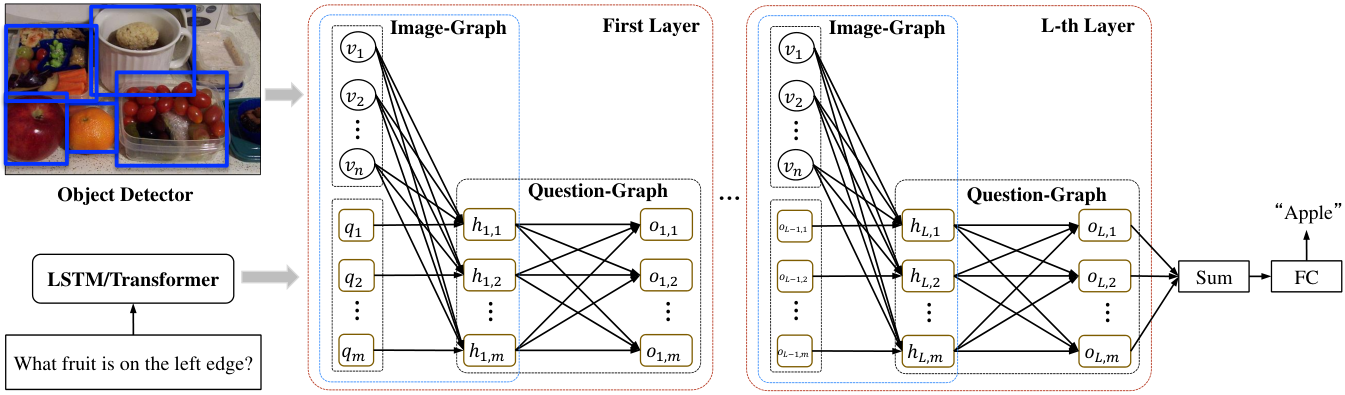
Even though Eqs. (8) and (9) provide an elegant approach to investigate the relationship between question features and image features , a simply summarization over columns of in Eq. (9) cannot fully address the connections between the joint embeddings corresponding to words. Given the question and image in Figure 1, BAN (i.e. Eqs. (8) and (9)) can locate a variety of fruits in the image according to the word ‘fruit’ in the question, but it is unaware of the relative position of each fruit from others by mixing all the information (i.e. the summarization in Eq. (9)), thus we want each joint embeddings to extract its related information from other items instead of an overall representation. Hence, we are motivated to develop bilinear graph networks, as shown in Figure 1, which has two kinds of graphs, i.e. image-graph and question-graph. The image-graph learns to build the relationship between words and objects and generates their joint embeddings, while the question-graph will update the joint embeddings in terms of words by exploiting their interactions.
We also find that the right answer may not be decided at once, therefore we stack our graphs to make the words interact with the objects as well as words themselves for multiple times.
Difference from other graph-based methods. Though we also investigate the VQA problem from a graph view, our model has several differences from existing graph-based methods. Compared with MUREL cadene2019murel, representing the question as a single vector to fuse with the image features at each step and emphasizing the relationship between objects, our method pays attention to modeling the relationship between words and objects as well as between words and words. Regarding DFAF gao2019dynamic, MCAN yu2019deep, and Vilbert lu2019vilbert, all of them use the scaled dot-product vaswani2017attention to model the graph weight between image and question as well as linearly combining both features to compute their join embeddings, which is less effective in modeling the representation of multi-modal inputs. We reformulate BAN as a bilinear graph between question and image and reveal its disadvantages, then we propose the image-graph and question-graph to solve it, which has a better explanation.
4.1 Image-Graph

The major target of the image-graph is to locate the objects related to semantic information of each word in the question. Beginning with Eq. (8), we have a multi-glimpse extension as shown in Figure 2.
Consider the graph , where and are the set of nodes and edges respectively. The image-graph has and , where are textual features of the question and are visual features of the detected objects, and are the computed graph weights based on and . To joint model the graph between image and question from different representation subspaces, we extend to multiple glimpses following kim2018bilinear; vaswani2017attention, resulting in , where is the number of glimpse. The -th graph attention is computed as:
| (10) |
where the parameters and are shared among glimpses except for , which can be seen from the upper part of Figure 2. After learning the graph attention, we use Eq. (8) to generate the joint embeddings as:
| (11) |
where represents the output of image-graph at glimpse .
Instead of concatenation vaswani2017attention; devlin2018bert; velickovic2017graph of joint embeddings from each glimpse, we follow BAN to use the residual form to integrate previous learned joint embeddings as shown in the lower part of Figure 2, then Eq. (11) becomes:
| (12) |
where , and projects the joint embeddings to the same dimension of . By convention, we use the output of the last glimpse to represent the whole image-graph, denoted as .
4.2 Question-Graph
For the question-graph, similarly, we have the graph nodes and graph weight , where are the output nodes of the image-graph, and are the self-attention graph weights of multiple glimpses based on denoted as:
| (13) |
The structure of our question-graph is similar to the image-graph in Figure 2, except that both inputs are . Different from Eq. (9), which summarizes the outputs from the image-graph based on to represent the whole graph, in Eq. (13) learns the context of each node for exchanging their information. Based on the graph weight , nodes of the question-graph at glimpse gather information from others and are represented as Eq. (12):
| (14) |
where and . The outputs of question-graph , abbreviated version of , can be utilized to answer the question by summarizing all the nodes to represent the whole graph.
As we mentioned above, the question may be compositional and complex that needs multi-step reasoning, thus we form the basic module of our bilinear graph networks with one image-graph following by one question-graph, and we stack the module for multiple layers to compose our framework shown in Figure 1. The first layer of the image-graph takes textual nodes as query to locate the related visual information in and outputs their joint nodes , and the higher layer of it takes the outputs of layer of the question-graph, , as query to involve more visual information related to the prior knowledge. The layer of question-graph aims at exchanging the information between nodes of to model the context and gets for prior knowledge of image-graph or answer prediction.
After stacking layers of bilinear graph networks, we summarize all the nodes of to represent the whole graph and pass it to a two-layer MLP for classification:
| (15) |
where , and is the size of .
5 Experiments
In this section, we evaluate our bilinear graph networks on VQA v2.0 dataset antol2015vqa; goyal2017making. We first introduce this dataset and then describe our implementation details and results, and finally the qualitative analysis.
5.1 Dataset
VQA v2.0 dataset: The dataset was built based on the MSCOCO images lin2014microsoft, and it contains 1.1M questions asked by human and each question is annotated by ten people. Compared with v1.0 dataset antol2015vqa, it emphasizes the visual understanding by reducing the text bias. The dataset is split into three parts: training, validation, and test, which have 80k images and 444 questions, 40k images and 214k questions, and 80k images and 448k questions respectively. The answers of the training and validation dataset are published for training model, while those of the test dataset are unknown and should be predicted by the proposed model before being uploaded to the server for performance evaluation. Based on the answer category, the questions can be classified into three types, i.e. yes/no, number, and others. We train our models with different settings on training dataset and evaluate their accuracy on validation dataset by the tools from antol2015vqa, then we pick the settings of the best model for training on the training and validation dataset with extra data from Visual Genome krishna2017visual that has 108k images and 1M questions, reporting results on test-server.
5.2 Implementation Details
We construct the answer vocabulary by restricting to the words that appear in the training and validation dataset more than eight times, resulting in . We then truncate or pad a question’s length to 15 words, and the weight of padding tokens in question-graph will be set to before softmax to reduce its impact. There are two methods to encode the question, one is LSTM, and the other one is Transformer. For the former one, we pass the question through a one-layer LSTM, whose input dimension of each word is 600, 300 of which is learned by our model and another 300 from pre-trained GloVe vector pennington2014glove is fixed, and the output dimension is 1,024. For the latter one, we encode the words by summing their corresponding token embeddings and position embeddings and project the outputs of the last layer of Transformer into vectors with dimension following by , where . We extract object features from a Faster-RCNN model anderson2018bottom pre-trained on Visual Genome, which has 1,600 object classes. For each image, we obtain top objects based on their probabilities with their object features and regions, and each object feature is presented by mean-pooling of their convolutional features with . The joint embedding size and are set to 1,024, and the rank is set to 3 during computing the graph attention weights in the image-graph and question-graph to increase its capacity. In order to save memory in each layer to make our network go deeper, we reduce the glimpse number from 8 (best performance in BAN) to . Weight Normalization salimans2016weight and Dropout srivastava2014dropout with are added after each linear mapping to stable the output and prevent from over-fitting. Due to the fact that there might exist multiple correct answers for a question, we utilize the binary cross-entropy loss (BCE) as loss function, which is calculated as:
| (16) |
where , and is the sigmoid function denoted as . Adamax kingma2014adam, a variant of Adam, is used to optimize our model. The initial learning rate is 0.001 and grows by 0.001 every epoch until reaching 0.004 for warm start, keeps constant until the eleventh epoch and decays by 1/4 every two epochs to 0.00025. The batch size is 128.
5.3 Ablation Study
We conduct several ablation studies to verify the contribution of each module in our bilinear graph networks (BGNs). The first four lines in Table 1 show the accuracy of BAN on the VQA v2.0 validation dataset, and BAN-4 and BAN-8 represent the model with 4 and 8 glimpses respectively. It can be seen that simply stacking the module of BAN can improve the accuracy to some extent (0.35% and 0.46% in the two-layer and three-layer model respectively) compared with the one-layer model. Although the multi-layer BAN might gain more visual information related to the global representation in Eq. (9) without exchanging context information, it is not clear about the relationship between entities in question. In contrast, our one-layer model, BGNs 1, gains an accuracy 0.62% and 0.43% higher than BAN-4 1 and BAN-8 1 respectively, proving the effectiveness of our proposed question-graph even with fewer glimpse. However, if we only stack the question-graph for multiple times (V-graph + Q-graph 2 and V-graph + Q-graph 3) with only one-layer image-graph, the performance grows slower than that of the BGNs 2, this might be caused by that the question-graph can only propagate the information already learned by the image-graph but cannot involve more factual information required in the image to answer the questions. If we replace the proposed bilinear graph network in question-graph with the scaled dot-production (SDP), the accuracy declines (-0.06% and -0.41% than BGNs with the same layer) and grows slightly (0.09%) by stacking the graph. It can be explained that though the inputs of question-graph are the same type of nodes, the nodes themselves are hybrid and the linear method cannot fully express their relations. By stacking three layers of the BGNs, our model achieves 67.21% on the overall accuracy, which is chosen as the best model.
| Model | VQA Score |
|---|---|
| BAN-4 1 | 65.81 |
| BAN-4 2 | 66.16 |
| BAN-4 3 | 66.27 |
| BAN-8 1 | 66.00 |
| BGNs 1 | 66.43 |
| V-graph + Q-graph 2 | 66.69 |
| V-graph + Q-graph 3 | 66.73 |
| (V-graph + SDP) 1 | 66.37 |
| (V-graph + SDP) 2 | 66.46 |
| BGNs 2 | 66.87 |
| BGNs 3 | 67.21 |
| BGNs 4 | 67.06 |
Additionally, we investigate the absolute increase of the score of our models compared with the single-layer BAN on questions with varied lengths to show the ability of our model on multi-step reasoning in Figure 3. Our models with different layers outperform the one-layer BAN, especially on long questions. The one-layer model does not perform as well as the other three models for long questions due to its shallow graphs. With more layers, our model becomes better at long questions and achieves a 1.7% increase at word number of nine. What interests us is why the performance drops at four-layer. Comparing the three-layer model and four-layer model, the former one works better in short questions (word number 8) which take 79% of all questions, while the latter one has a higher score in long questions, this may explain the performance drop. This phenomenon also inspires us to design a network in the future to classify the questions to fit different layers of graphs.
| Model | VQA Score | |
|---|---|---|
| BGNs 1 + LSTM | 1 | 66.43 |
| BGNs 1 + Base | 0 | 66.52 |
| BGNs 1 + Base | 0.001 | 67.62 |
| BGNs 1 + Base | 0.01 | 68.09 |
| BGNs 1 + Base | 0.1 | 67.84 |
| BGNs 1 + Large | 0.01 | 68.20 |
| BGNs 2 + Large | 0.01 | 68.50 |
| BGNs 3 + Large | 0.01 | 68.71 |
Furthermore, we explore the influence of BERT devlin2018bert on our method, since it is trained on large text corpus, therefore it has better generalization and representation of textual features. So we replace the LSTM with it when modeling the question and fine-tuning its weight with different strategies. By using the base model of BERT without fine-tuning (BGNs 1 + Base with ), the accuracy increases slightly, and by increasing its learning rate, it boosts and achieves the best performance at . With this learning rate, we switch to the large model that is deeper and wider than the base one, the performance grows and keeps going by stacking our bilinear graph model on it, proving that our model is effective and compatible with BERT.


5.4 Comparison with State-of-the-Art
| Model | Overall | Yes/no | Number | Other | Test-std |
|---|---|---|---|---|---|
| Bottom-Up anderson2018bottom | 65.32 | 81.82 | 44.21 | 56.05 | 65.67 |
| Counter zhang2018learning | 68.09 | 83.14 | 51.62 | 58.97 | 68.41 |
| MuRel cadene2019murel | 68.03 | 84.77 | 49.84 | 57.85 | 68.41 |
| MFH+Bottom-Up yu2018beyond | 68.76 | 84.27 | 49.56 | 59.89 | - |
| BAN+Glove kim2018bilinear | 69.66 | 85.46 | 50.66 | 60.60 | - |
| BAN+Glove+Counter kim2018bilinear | 70.04 | 85.42 | 54.04 | 60.52 | 70.35 |
| DFAF gao2019dynamic | 70.22 | 86.09 | 53.32 | 60.49 | 70.34 |
| Vilbert lu2019vilbert | 70.55 | - | - | - | 70.92 |
| MCAN yu2019deep | 70.63 | 86.82 | 53.26 | 60.72 | 70.90 |
| MLIN gao2019multi | 70.18 | 85.96 | 52.93 | 60.40 | 70.28 |
| BGNs+Glove+Counter (ours) | 71.00 | 86.62 | 56.31 | 60.95 | - |
| BGNs+Glove (ours) | 70.97 | 87.03 | 53.56 | 61.18 | 71.12 |
| DFAF+BERT gao2019dynamic | 70.59 | 86.73 | 52.92 | 61.04 | 70.81 |
| MLIN+BERT gao2019multi | 71.09 | 87.07 | 53.39 | 60.49 | 71.27 |
| BGNs+BERT (ours) | 72.28 | 88.60 | 54.09 | 62.46 | 72.41 |
In Table 3, we evaluate our method on VQA v2.0 test-dev dataset, which achieves state-of-the-art. As shown in Table 3, the overall accuracy of our BGNs+Glove model is 1.31% higher than BAN+Glove, nearly 3.0% on number metric. It can be explained that the counting task is a kind of relation among objects, which tries to find similar objects in the latter layers with objects grounded by previous layers. And the extra counter module zhang2018learning in our BGNs+Glove+Counter model makes a little gain on overall accuracy since it might increase the counting ability but disturb our reasoning graphs leading to drop in other metrics. Thus, we choose BGNs+Glove and BGNs+BERT as our best models to evaluate them on the test-standard dataset.
As we mentioned in Section 4, our bilinear graph networks have a better explanation in modeling the relationship within multi-modal inputs, and we also achieve better performance on both test-dev and test-std dataset compared with other methods with and without BERT, proving the effectiveness of our proposed method.
5.5 Qualitative Analysis

To visualize the effects of each module in our bilinear graph networks, we present the learned attention maps of the image-graph and the question-graph in each layer to show how the networks work. Given the question ‘What fruit is on the left edge?’ in Figure 4, the image-graph of the first layer attends kinds of objects in the input image, while the question-graph broadcasts the learned fruit information to other words and chooses ‘tomato’ as the answer, probably because the amount of ‘tomato’ is the biggest among all detected fruits. The image-graph of the second-layer picks ‘orange’ that is to the left of ‘tomato’ and the question-graph keeps collecting ‘fruit’ and ‘edge’ information. In the third layer, the image-graph locates ‘apple’ that is on the left edge, and every word in the question-graph pays its attention to the ‘edge’ information to predict the answer.
In Figure 5, we show the answer predicted by BAN and our models with one layer, two layers, and three layers. In the first image of the top row, BAN cannot correctly answer the question because the entities of ‘young girl’ and ‘bag’ learn their positions respectively, but they do not know each other’s information, while our proposed question-graph exchanges such positional information to make it possible to compare the relative direction of the two entities. A similar question can also be found in the first image of the bottom row, our model approaches the correct answer step by step as the layer of the graph increases. Moreover, our model can find the implicit relationship between objects, even when the sheep are far away from the dog in the second image of the top row, as well as abstract scenes in the second image (five circles representing Olympics) and third image (many trees composing forest) of the bottom row. Furthermore, our model finely discriminates the highly overlapped objects, such as two sheep in the second image and the rope in the fourth image of the top row, it is possibly because the question-graph undertakes some burden from the original graph of BAN, which makes the image-graph spare more effort on learning details in the image.
6 Conclusions
Motivated by graph attention networks and Transformer, in this paper, we interpret bilinear attention networks from a new perspective and demonstrate its disadvantages, then we develop bilinear graph networks (BGNs) composed of layers of image-graph and question-graph to overcome them. The image-graph learns the graph between words in the question and objects in the image and generate the joint embeddings of them, while the question-graph models the graph between these joint embeddings in term of words to exchange context information. Our method achieves state-of-the-art performance on VQA v2.0 dataset, and the ablation studies show that our bilinear graph networks significantly outperform the BAN and other graph-based methods on a variety of questions.
References
- (1) Peter Anderson, Xiaodong He, Chris Buehler, Damien Teney, Mark Johnson, Stephen Gould, and Lei Zhang. Bottom-up and top-down attention for image captioning and visual question answering. In CVPR, volume 3, page 6, 2018.
- (2) Stanislaw Antol, Aishwarya Agrawal, Jiasen Lu, Margaret Mitchell, Dhruv Batra, C Lawrence Zitnick, and Devi Parikh. Vqa: Visual question answering. In Proceedings of the IEEE international conference on computer vision, pages 2425–2433, 2015.
- (3) Remi Cadene, Hedi Ben-Younes, Matthieu Cord, and Nicolas Thome. Murel: Multimodal relational reasoning for visual question answering. In Proceedings of the IEEE Conference on Computer Vision and Pattern Recognition, pages 1989–1998, 2019.
- (4) Yunpeng Chen, Marcus Rohrbach, Zhicheng Yan, Yan Shuicheng, Jiashi Feng, and Yannis Kalantidis. Graph-based global reasoning networks. In Proceedings of the IEEE Conference on Computer Vision and Pattern Recognition, pages 433–442, 2019.
- (5) Junyoung Chung, Caglar Gulcehre, KyungHyun Cho, and Yoshua Bengio. Empirical evaluation of gated recurrent neural networks on sequence modeling. arXiv preprint arXiv:1412.3555, 2014.
- (6) Abhishek Das, Satwik Kottur, Khushi Gupta, Avi Singh, Deshraj Yadav, José MF Moura, Devi Parikh, and Dhruv Batra. Visual dialog. In Proceedings of the IEEE Conference on Computer Vision and Pattern Recognition, volume 2, 2017.
- (7) Jacob Devlin, Ming-Wei Chang, Kenton Lee, and Kristina Toutanova. Bert: Pre-training of deep bidirectional transformers for language understanding. arXiv preprint arXiv:1810.04805, 2018.
- (8) Akira Fukui, Dong Huk Park, Daylen Yang, Anna Rohrbach, Trevor Darrell, and Marcus Rohrbach. Multimodal compact bilinear pooling for visual question answering and visual grounding. arXiv preprint arXiv:1606.01847, 2016.
- (9) Peng Gao, Zhengkai Jiang, Haoxuan You, Pan Lu, Steven CH Hoi, Xiaogang Wang, and Hongsheng Li. Dynamic fusion with intra-and inter-modality attention flow for visual question answering. In Proceedings of the IEEE Conference on Computer Vision and Pattern Recognition, pages 6639–6648, 2019.
- (10) Peng Gao, Haoxuan You, Zhanpeng Zhang, Xiaogang Wang, and Hongsheng Li. Multi-modality latent interaction network for visual question answering. arXiv preprint arXiv:1908.04289, 2019.
- (11) Yash Goyal, Tejas Khot, Douglas Summers-Stay, Dhruv Batra, and Devi Parikh. Making the v in vqa matter: Elevating the role of image understanding in visual question answering. In Proceedings of the IEEE Conference on Computer Vision and Pattern Recognition, pages 6904–6913, 2017.
- (12) Dalu Guo, Chang Xu, and Dacheng Tao. Image-question-answer synergistic network for visual dialog. In Proceedings of the IEEE Conference on Computer Vision and Pattern Recognition, pages 10434–10443, 2019.
- (13) Will Hamilton, Zhitao Ying, and Jure Leskovec. Inductive representation learning on large graphs. In Advances in Neural Information Processing Systems, pages 1024–1034, 2017.
- (14) Kaiming He, Xiangyu Zhang, Shaoqing Ren, and Jian Sun. Deep residual learning for image recognition. In Proceedings of the IEEE conference on computer vision and pattern recognition, pages 770–778, 2016.
- (15) Sepp Hochreiter and Jürgen Schmidhuber. Long short-term memory. Neural computation, 9(8):1735–1780, 1997.
- (16) Jin-Hwa Kim, Jaehyun Jun, and Byoung-Tak Zhang. Bilinear attention networks. arXiv preprint arXiv:1805.07932, 2018.
- (17) Jin-Hwa Kim, Kyoung-Woon On, Woosang Lim, Jeonghee Kim, Jung-Woo Ha, and Byoung-Tak Zhang. Hadamard product for low-rank bilinear pooling. arXiv preprint arXiv:1610.04325, 2016.
- (18) Diederik P Kingma and Jimmy Ba. Adam: A method for stochastic optimization. arXiv preprint arXiv:1412.6980, 2014.
- (19) Thomas N Kipf and Max Welling. Semi-supervised classification with graph convolutional networks. arXiv preprint arXiv:1609.02907, 2016.
- (20) Ranjay Krishna, Yuke Zhu, Oliver Groth, Justin Johnson, Kenji Hata, Joshua Kravitz, Stephanie Chen, Yannis Kalantidis, Li-Jia Li, David A Shamma, et al. Visual genome: Connecting language and vision using crowdsourced dense image annotations. International Journal of Computer Vision, 123(1):32–73, 2017.
- (21) Tsung-Yi Lin, Michael Maire, Serge Belongie, James Hays, Pietro Perona, Deva Ramanan, Piotr Dollár, and C Lawrence Zitnick. Microsoft coco: Common objects in context. In European conference on computer vision, pages 740–755. Springer, 2014.
- (22) Yong Liu, Ruiping Wang, Shiguang Shan, and Xilin Chen. Structure inference net: Object detection using scene-level context and instance-level relationships. In Proceedings of the IEEE conference on computer vision and pattern recognition, pages 6985–6994, 2018.
- (23) Jiasen Lu, Dhruv Batra, Devi Parikh, and Stefan Lee. Vilbert: Pretraining task-agnostic visiolinguistic representations for vision-and-language tasks. arXiv preprint arXiv:1908.02265, 2019.
- (24) Hyeonseob Nam, Jung-Woo Ha, and Jeonghee Kim. Dual attention networks for multimodal reasoning and matching. arXiv preprint arXiv:1611.00471, 2016.
- (25) Jeffrey Pennington, Richard Socher, and Christopher D. Manning. Glove: Global vectors for word representation. In Empirical Methods in Natural Language Processing (EMNLP), pages 1532–1543, 2014.
- (26) Shaoqing Ren, Kaiming He, Ross Girshick, and Jian Sun. Faster r-cnn: Towards real-time object detection with region proposal networks. In Advances in neural information processing systems, pages 91–99, 2015.
- (27) Tim Salimans and Durk P Kingma. Weight normalization: A simple reparameterization to accelerate training of deep neural networks. In Advances in Neural Information Processing Systems, pages 901–909, 2016.
- (28) Nitish Srivastava, Geoffrey Hinton, Alex Krizhevsky, Ilya Sutskever, and Ruslan Salakhutdinov. Dropout: a simple way to prevent neural networks from overfitting. The Journal of Machine Learning Research, 15(1):1929–1958, 2014.
- (29) Ashish Vaswani, Noam Shazeer, Niki Parmar, Jakob Uszkoreit, Llion Jones, Aidan N Gomez, Łukasz Kaiser, and Illia Polosukhin. Attention is all you need. In Advances in Neural Information Processing Systems, pages 5998–6008, 2017.
- (30) Petar Velickovic, Guillem Cucurull, Arantxa Casanova, Adriana Romero, Pietro Lio, and Yoshua Bengio. Graph attention networks. arXiv preprint arXiv:1710.10903, 1(2), 2017.
- (31) Xiaolong Wang, Ross Girshick, Abhinav Gupta, and Kaiming He. Non-local neural networks. In Proceedings of the IEEE Conference on Computer Vision and Pattern Recognition, pages 7794–7803, 2018.
- (32) Jianwei Yang, Jiasen Lu, Stefan Lee, Dhruv Batra, and Devi Parikh. Graph r-cnn for scene graph generation. In Proceedings of the European Conference on Computer Vision (ECCV), pages 670–685, 2018.
- (33) Zichao Yang, Xiaodong He, Jianfeng Gao, Li Deng, and Alex Smola. Stacked attention networks for image question answering. In Proceedings of the IEEE Conference on Computer Vision and Pattern Recognition, pages 21–29, 2016.
- (34) Zhou Yu, Jun Yu, Yuhao Cui, Dacheng Tao, and Qi Tian. Deep modular co-attention networks for visual question answering. In Proceedings of the IEEE Conference on Computer Vision and Pattern Recognition, pages 6281–6290, 2019.
- (35) Zhou Yu, Jun Yu, Jianping Fan, and Dacheng Tao. Multi-modal factorized bilinear pooling with co-attention learning for visual question answering. IEEE International Conference on Computer Vision (ICCV), pages 1839–1848, 2017.
- (36) Zhou Yu, Jun Yu, Chenchao Xiang, Jianping Fan, and Dacheng Tao. Beyond bilinear: generalized multimodal factorized high-order pooling for visual question answering. IEEE transactions on neural networks and learning systems, (99):1–13, 2018.
- (37) Zhou Yu, Jun Yu, Chenchao Xiang, Zhou Zhao, Qi Tian, and Dacheng Tao. Rethinking diversified and discriminative proposal generation for visual grounding. arXiv preprint arXiv:1805.03508, 2018.
- (38) Yan Zhang, Jonathon Hare, and Adam Prügel-Bennett. Learning to count objects in natural images for visual question answering. arXiv preprint arXiv:1802.05766, 2018.