Consistent model selection criteria and goodness-of-fit test for affine causal processes

Jean-Marc Bardet Kare Kamila^?? William Kengne

Abstract

This paper studies the model selection problem in a large class of causal time series models, which includes both the ARMA or AR( $\infty$ ) processes, as well as the GARCH or ARCH( $\infty$ ), APARCH, ARMA-GARCH and many others processes. To tackle this issue, we consider a penalized contrast based on the quasi-likelihood of the model. We provide sufficient conditions for the penalty term to ensure the consistency of the proposed procedure as well as the consistency and the asymptotic normality of the quasi-maximum likelihood estimator of the chosen model. It appears from these conditions that the Bayesian Information Criterion (BIC) does not always guarantee the consistency. We also propose a tool for diagnosing the goodness-of-fit of the chosen model based on the portmanteau Test. Numerical simulations and an illustrative example on the FTSE index are performed to highlight the obtained asymptotic results, including a numerical evidence of the non consistency of the usual BIC penalty for order selection of an AR $(p)$ models with ARCH( $\infty$ ) errors.

keywords

[class=MSC] Primary 60K35 , 60K35 ; secondary 60K35

keywords

model selection , affine causal processes , consistency , BIC , Portmanteau Test

and

S.A.M.M., Université Paris 1, Panthéon-Sorbonne,
90, rue de Tolbiac, 75634, Paris, France
??

THEMA, Université de Cergy-Pontoise, FRANCE.
??

1 Introduction

Model selection is an important tool for statisticians and all those who process data. This issue has received considerable attention in the recent literature. There are several model selection procedures, the main ones are : cross validation and penalized contrast based.

The cross validation ([43], [2]) consists in splitting the data into learning sample, which will be used for computing estimators of the parameters and the test sample which allows to assess these estimators by evaluate their risks.

The procedures using penalized objective function search for a model, minimizing a trade-off between a sum of an empirical risk (for instance least squares, $-2\times$ log-likelihood), which indicates how well the model fits the data, and a measure of model’s complexity so-called a penalty.
The idea of penalizing dates back to the 1970s with the works of [34] and [1]. By using the ordinary least squares in regression framework, Mallows obtained the $C_{p}$ criterion. Meanwhile, Akaike derived AIC for density estimation using log-likelihood contrast. A few years later, following Akaike, [38] proposed an alternative approach to density estimation and derived the Bayesian Information Criteria (BIC). The penalty term of these criteria is proportional to the dimension of the model. In the recent decades, different approaches of penalization have emerged such as the $\mathbb{L}^{2}$ norm for the Ridge penalisation [18], the $\mathbb{L}^{1}$ norm used by [45] that provides the LASSO procedure and the elastic-net that mixes the $\mathbb{L}^{1}$ and $\mathbb{L}^{2}$ norms [50].

Model selection procedures can have two different objectives: consistency and efficiency. A procedure is said to be consistent if given a family of models, including the ”true model”, the probability of choosing the correct model approaches one as the sample size tends to infinity. On the other hand, a procedure is efficient when its risk is asymptotically equivalent to the risk of the oracle. In this work, we are interested to construct a consistent procedure for the general class of times series known as affine causal processes.

This class of affine causal time series can be defined as follows. Let $\mathbb{R}^{\infty}$ be the space of sequences of real numbers with a finite number of non zero, if $M$ , $f$ : $\mathbb{R}^{\infty}\to\mathbb{R}$ are two measurable functions, then an affine causal class is

Class $\mathcal{AC}(M,f):$ A process $X=(X_{t})_{t\in\mathbb{Z}}$ belongs to $\mathcal{AC}(M,f)$ if it satisfies:

X_{t}=M\big((X_{t-i})_{i\in\mathbb{N}^{*}}\big)\,\xi_{t}+f\big((X_{t-i})_{i\in\mathbb{N}^{*}}\big)\;\;\mbox{for any}\penalty\ t\in\mathbb{Z};

(1.1)

where $(\xi)_{t\in\mathbb{Z}}$ is a sequence of zero-mean independent identically distributed random vectors (i.i.d.r.v) satisfying $\mathbb{E}(|\xi_{0}|^{r})<\infty$ for some $r\geq 2$ and $\mathbb{E}[\xi_{0}^{2}]=1$ .

For instance,

•

if $M\big((X_{t-i})_{i\in\mathbb{N}^{*}}\big)=\sigma$ and $f\big((X_{t-i})_{i\in\mathbb{N}^{*}}\big)=\phi_{1}X_{t-1}+\cdots+\phi_{p}X_{t-p}$ , then $(X_{t})_{t\in\mathbb{Z}}$ is an AR $(p)$ process;
•

if $M\big((X_{t-i})_{i\in\mathbb{N}^{*}}\big)=\sqrt{a_{0}+a_{1}X^{2}_{t-1}+\cdots+a_{p}X^{2}_{t-p}}$ and $f\big((X_{t-i})_{i\in\mathbb{N}^{*}}\big)=0$ , then $(X_{t})_{t\in\mathbb{Z}}$ is an ARCH $(p)$ process.

Note that, numerous classical time series models such as ARMA( $p,q$ ), GARCH( $p,q$ ), ARMA( $p,q$ )-GARCH( $p,q$ ) (see [12] and [33]) or APARCH $(\delta,p,q)$ processes (see [12]) belongs to $\mathcal{AC}(M,f)$ . The existence of stationary and ergodic solutions of this class has been studied in [13] and [7].

We consider a trajectory $(X_{1},\ldots,X_{n})$ of a stationary affine causal process $\mathcal{AC}(M^{*},f^{*})$ , where $M^{*}$ and $f^{*}$ are unknown. We also consider a finite set ${\cal M}$ of parametric models $m$ , which are affine causal time series. We assume that the ”true” model $m^{*}$ corresponds to $M^{*}$ and $f^{*}$ . The aim is to obtain an estimator $\widehat{m}$ of $m^{*}$ and testing the goodness-of-fit of the chosen model.

There already exist several important contributions devoted to the model selection for time series ; we refer to the book of [35] and the references therein for an overview on this topic.
As we have pointed above, two properties are often used to evaluate a quality of a model selection procedure : consistency and efficiency. The first measure is often used when the true model is included in the collection of model’s candidate ; otherwise, efficiency is the well-defined property. In many research in this framework, the main goal is to develop a procedure that fulfills one of these properties. So, in some classical linear time series models, the consistency of the BIC procedure has been established, see for instance [17] or [46] ; and the asymptotic efficiency of the AIC has been proved, see, among others, [41], [20] for a corrected version of AIC for small samples, [23], [21], [22] for the case of infinite order autoregressive model. [40] propose the (consistent) residual information criteria (RIC) for regression model (including regression models with ARMA errors) selection. In the framework of nonlinear threshold models, [25] proved consistency results of a large class of information criteria, whereas [16] focussed on cross-validation type procedure for model selection in a class of semiparametric time series regression model. Let us recall that, the time series model selection literature is very extensive and still growing ; we refer to the monograph of [36], which provided an excellent summary of existing model selection procedure, including the case of time series models as well as the recent review paper of [11].

The adaptive lasso, introduced by [49] for variable selection in linear regression models has been extended by [37] to vector autoregressive models, [26] carried out this procedure in stationary and nonstationary autoregressive models ; the oracle efficient is established. [28] considers model selection for density estimation under mixing conditions and derived oracle inequalities of the slope heuristic procedure ([9] or [5]) ; whereas [3] develop oracle inequalities for model selection for weakly dependent time series forecasting. Recently, [39] have considered the model selection for ARMA time series with trend, and proved the consistency of BIC for the detrended residual sequence, while [4] developed oracle inequalities of sequential model selection method for nonparametric autoregression. [19] pointed out that most existing model selection procedure cannot simultaneously enjoy consistency and (asymptotic) efficiency. They propose a misspecification-resistant information criterion that can achieve consistency and asymptotic efficiency for prediction using model selection.

In this paper, we focus on the class of models (1.1), and addressed the following questions :

1.

What regularity conditions are sufficient to build a consistent model selection procedure? Does the classic criterion such as BIC, still have consistent property for choosing a model among the collections $\mathcal{M}$ ?
2.

How can we test the goodness-of-fit of the chosen model?

These questions have not yet been answered for the class of models and the framework considered here, in particular in case of infinite memory processes. This new contribution provides theoretical and numerical response of these issues.

(i) The estimator $\widehat{m}$ of $m^{*}$ is chosen by minimizing a penalized criterion $\widehat{C}(m)=-2\widehat{L}_{n}(m)+|m|\,\kappa_{n}$ , where $\widehat{L}_{n}(m)$ is a Gaussian quasi-log-likelihood of the model $m$ , $|m|$ is the number of estimated parameters of the model $m$ and $\kappa_{n}$ is a non-decreasing sequence of real numbers (see more details in Section 2). Note that, in the cases $\kappa_{n}=2$ or $\kappa_{n}=\log n$ we respectively consider the usual AIC and BIC criteria. We provide sufficient conditions (essentially depending on the decreasing of the Lipschitz coefficients of the functions $f$ and $M$ ) for obtaining consistency of the model selection procedure. We also theoretically and numerically exhibit an example of order selection (weak AR $(p)$ processes with ARCH( $\infty$ ) errors) such that the consistency of the classical BIC penalty is not ensured.

(ii) We provide an asymptotic goodness-of-fit test for the selected model that is very simple to be used (with the usual Chi-square distribution limit), which successively completes the model selection procedure. Numerical applications show the accuracy of this test under the null hypothesis as well as an efficient test power under an alternative hypothesis. Note that, similar test has been proposed by [31] under the Gaussian assumption on the observations, whereas [32] focused for multivariate time series with multivariate ARCH-type errors. Also, [14] proposed a portmanteau test statistic based on generalized inverses and $\{2\}$ -inverses for diagnostic checking in the class of model (1.1). Unlike these authors, we apply the test to a model obtained from a model selection procedure.

The paper is organized as follows. Some definitions, notations and assumptions are described in Section 2. The consistency of the criteria and the asymptotic normality of the post-model-selection estimator are studied in Section 3. In Section 4, the examples of $AR(\infty)$ , $ARCH(\infty)$ , $APARCH(\delta,p,q)$ and ARMA $(p,q)$ -GARCH $(p^{\prime},q^{\prime})$ processes are detailed. The goodness-of-fit test is presented in Section 5. Finally, numerical results are presented in Section 6 and Section 7 contains the proofs.

2 Definitions and Assumptions

Let us introduce some definitions and assumptions in order to facilitate the presentation.

2.1 Notation and assumptions

In the sequel, we will consider a subset $\Theta$ of $\mathbb{R}^{d}$ ( $d\in\mathbb{N}$ ). We will use the following norms:

•

$\|.\|$ denotes the usual Euclidean norm on $\mathbb{R}^{\nu}$ , with $\nu\geq 1$ ;
•

if $X$ is $\mathbb{R}^{\nu}$ -random variable with $r\geq 1$ order moment, we set $\|X\|_{r}=\big(\mathbb{E}(\|X\|^{r}\big)^{1/r}$ ;
•

for any set $\Theta\subseteq\mathbb{R}^{d}$ and for any $g:\Theta\to\mathbb{R}^{d^{\prime}}$ , $d^{\prime}\geq 1$ , denote $\|g\|_{\Theta}=\underset{\theta\in\Theta}{\sup}\big\{\|g(\theta)\|\big\}$ .

In the introduction, to be more concise, we have presented the problem of time series model selection in a very general form. In reality, we will limit our field of study a little bit by considering a semi-parametric framework. Hence, let $(f_{\theta})_{\theta\in\Theta}$ and $(M_{\theta})_{\theta\in\Theta}$ be two families of known functions such as for any $\theta\in\Theta$ , both $f_{\theta},M_{\theta}$ with real values defined on $\mathbb{R}^{\infty}$ .

We begin by giving a condition on $f_{\theta}$ and $M_{\theta}$ which ensure the existence of a $r$ -order moment, stationary and ergodic time series belonging to $\mathcal{AC}(M_{\theta},f_{\theta})$ . This condition, initially obtained in [13], is written in terms of Lipschitz coefficients of both these functions. Hence, for $\Psi_{\theta}=f_{\theta}$ or $M_{\theta}$ , define:

Assumption A $(\Psi_{\theta},\Theta)$ : Assume that $\|\Psi_{\theta}(0)\|_{\Theta}<\infty$ and there exists a sequence of non-negative real numbers $\big(\alpha_{k}(\Psi_{\theta},\Theta)\big)_{k\geq 1}$ such that $\sum_{k=1}^{\infty}\alpha_{k}(\Psi_{\theta},\Theta)<\infty$ satisfying:

\|\Psi_{\theta}(x)-\Psi_{\theta}(y)\|_{\Theta}\leq\sum_{k=1}^{\infty}\alpha_{k}(\Psi_{\theta},\Theta)|x_{k}-y_{k}|\;for\;all\;x,y\in\mathbb{R}^{\mathbb{\infty}}.

Now for $r\geq 1$ , where $\|\xi_{0}\|_{r}<\infty$ , define:

\Theta(r)=\Big\{\theta\in\mathbb{R}^{d},\penalty\ A(f_{\theta},\{\theta\})\;\textnormal{and}\;A(M_{\theta},\{\theta\})\;\textnormal{hold with}\\ \sum_{k=1}^{\infty}\alpha_{k}(f_{\theta},\{\theta\})+\|\xi_{0}\|_{r}\,\sum_{k=1}^{\infty}\alpha_{k}(M_{\theta},\{\theta\})<1\Big\}.

(2.1)

Then, for any $\theta\in\Theta(r)$ , there exists a stationary and ergodic solution with $r$ -order moment belonging to $\mathcal{AC}(M_{\theta},f_{\theta})$ . (see [13] and [7]).

2.2 The framework

Let us start with an example to better understand the framework and the approach of model selection we will follow.

Example: Assume that the observed trajectory $(X_{1},\ldots,X_{n})$ is generated from an AR $(2)$ process and we would like to identify this family of process and its order. Then, we consider the collection $\cal{M}$ of ARMA $(p,q)$ and GARCH $(p^{\prime},q^{\prime})$ processes for $0\leq p,q,p^{\prime},q^{\prime}\leq 9$ and we would like to chose in this family a ”best” model for fitting $(X_{1},\ldots,X_{n})$ . Note that there is $200$ possible models and we expect to recognize the AR $(2)$ as the selected model, at least when $n$ is large enough.

We begin with the following property that allow to enlarge the family of models by extending the dimension $d$ of the parameter $\theta$ :

Proposition 1.

Let $d_{1},d_{2}\in\mathbb{N}$ , $\Theta_{1}\subset\mathbb{R}^{d_{1}}$ and $\Theta_{2}\subset\mathbb{R}^{d_{2}}$ , and for $i=1,2$ , define $f_{\theta_{i}}^{(i)},M_{\theta_{i}}^{(i)}:\mathbb{R}^{\infty}\to\mathbb{R}$ and for $\theta_{i}\in\Theta_{i}$ . Then there exist $\max(d_{1},d_{2})\leq d\leq d_{1}+d_{2}$ , $\Theta\subset\mathbb{R}^{d}$ , and a family of functions $f_{\theta}:\mathbb{R}^{\infty}\to\mathbb{R}$ and $M_{\theta}:\mathbb{R}^{\infty}\to[0,\infty)$ with $\theta\in\Theta$ , such that for any $\theta_{1}\in\Theta_{1}$ and $\theta_{2}\in\Theta_{2}$ , there exists $\theta\in\Theta$ satisfying

\mathcal{AC}\big(M_{\theta_{1}}^{(1)},f_{\theta_{1}}^{(1)}\big)\bigcup\mathcal{AC}\big(M_{\theta_{2}}^{(2)},f_{\theta_{2}}^{(2)}\big)\subset\mathcal{AC}\big(M_{\theta},f_{\theta}\big).

The proof of this proposition, as well as the other proofs, can be found in Section 7. This proposition says that it is always possible to embed two parametric causal affine models in a larger one. Hence, for instance, we can consider as well AR processes and ARCH processes in a unique representation, i.e.

\left\{\begin{array}[]{ll}AR&\left\{\begin{array}[]{l}M_{\theta_{1}}^{(1)}\big((X_{t-i})_{i\in\mathbb{N}^{*}}\big)=\sigma\\ f_{\theta_{1}}^{(1)}\big((X_{t-i})_{i\in\mathbb{N}^{*}}\big)=\phi_{1}X_{t-1}+\cdots+\phi_{p}X_{t-p}\end{array}\right.\\ \\ ARCH&\left\{\begin{array}[]{l}M_{\theta_{2}}^{(2)}\big((X_{t-i})_{i\in\mathbb{N}^{*}}\big)=\sqrt{a_{0}+a_{1}X^{2}_{t-1}+\cdots+a_{q}X^{2}_{t-q}}\\ f_{\theta_{2}}^{(2)}\big((X_{t-i})_{i\in\mathbb{N}^{*}}\big)=0\end{array}\right.\end{array}\right.\\ \Longrightarrow\left\{\begin{array}[]{l}M_{\theta}\big((X_{t-i})_{i\in\mathbb{N}^{*}}\big)=\sqrt{\theta_{0}+\theta_{1}X^{2}_{t-1}+\cdots+\theta_{q}X^{2}_{t-q}}\\ f_{\theta}\big((X_{t-i})_{i\in\mathbb{N}^{*}}\big)=\theta_{q+1}X_{t-1}+\cdots+\theta_{q+p}X_{t-p}\end{array}\right..

From now and in all the sequel, we fix $d\in\mathbb{N}^{*}$ , and the family of functions $f_{\theta},M_{\theta}:\mathbb{R}^{\infty}\to\mathbb{R}$ for $\theta\in\Theta\subset\Theta(r)\subset\mathbb{R}^{d}$ .

Let $(X_{1},\ldots,X_{n})$ be an observed trajectory of an affine causal process $X$ belonging to $\mathcal{AC}(M_{\theta^{*}},f_{\theta^{*}})$ , where $\theta^{*}$ is an unknown vector of $\Theta$ , and therefore:

X_{t}=M_{\theta^{*}}\big((X_{t-i})_{i\in\mathbb{N}^{*}}\big)\,\xi_{t}+f_{\theta^{*}}\big((X_{t-i})_{i\in\mathbb{N}^{*}}\big)\;\;\mbox{for any}\penalty\ t\in\mathbb{Z}.

(2.2)

In the sequel, we will consider several models, which all are particular cases of $\mathcal{AC}(M_{\theta},f_{\theta})$ with $\theta\in\Theta\subset\mathbb{R}^{d}$ . More precisely define:

•

a model $m$ as a subset of $\{1,\ldots,d\}$ and denote $|m|=\#(m)$ ;
•

$\Theta(m)=\big\{(\theta_{i})_{1\leq i\leq d}\in\mathbb{R}^{d},\penalty\ \theta_{i}=0\penalty\ \mbox{if $i\notin m$}\big\}\cap\Theta$ ;
•

${\cal M}$ as a family of models, i.e. ${\cal M}\subset{\cal P}\big(\{1,\ldots,d\}\big)$ .

Finally, for all $m\in{\cal M}$ , $m\in\mathcal{AC}(M_{\theta},f_{\theta})$ when $\theta\in\Theta(m)$ and denote $m^{*}$ the ”true” model. We could as well consider hierarchical or exhaustive families of models.

Example: From the previous example, we can consider:
$\bullet$ a family ${\cal M}_{1}$ of models $m_{1}$ such as ${\cal M}_{1}=\big\{\{1\},\{1,2\},\ldots,\{1,\ldots,q+1\}\big\}$ : this family is the hierarchical one of ARCH processes with orders varying from $0$ to $q$ .
$\bullet$ a family ${\cal M}_{2}$ of models $m_{2}$ such as ${\cal M}_{2}={\cal P}\big(\{1,\ldots,p+q+1\}\big)$ : this family is the exhaustive one and contains as well the AR $(2)$ process $X_{t}=\phi_{2}X_{t-2}+\theta_{0}\,\xi_{t}$ as the process $X_{t}=\phi_{1}X_{t-1}+\phi_{3}X_{t-3}+\xi_{t}\,\sqrt{\theta_{0}+a_{2}X_{t-2}^{2}}$ .

To establish the consistency of the selected model, we will need to assume that the ”true” model $m^{*}$ with the parameter $\theta^{*}$ , is included in the model family ${\cal M}$ .

2.3 The special case of NLARCH $(\infty)$ processes

As in [7], in the special case of NLARCH $(\infty)$ processes, including for instance GARCH $(p,q)$ or ARCH $(\infty)$ processes, a particular treatment can be realized for obtaining sharper results than using the previous framework. In such case, define the class:

Class $\widetilde{\mathcal{AC}}(\widetilde{H}_{\theta})$ : A process $X=(X_{t})_{t\in\mathbb{Z}}$ belongs to $\widetilde{\mathcal{AC}}(\widetilde{H}_{\theta})$ if it satisfies:

X_{t}=\xi_{t}\,\sqrt{\widetilde{H}_{\theta}\big((X^{2}_{t-i})_{i\in\mathbb{N}^{*}}\big)}\;\;\mbox{for any}\penalty\ t\in\mathbb{Z}.

(2.3)

Therefore, if $M^{2}_{\theta}\big((X_{t-i})_{i\in\mathbb{N}^{*}}\big)=H_{\theta}\big((X_{t-i})_{i\in\mathbb{N}^{*}}\big)=\widetilde{H}_{\theta}\big((X^{2}_{t-i})_{i\in\mathbb{N}^{*}}\big)$ then, $\widetilde{\mathcal{AC}}(\widetilde{H}_{\theta})={\mathcal{AC}}(M_{\theta},0)$ . In case of the class $\widetilde{\mathcal{AC}}(\widetilde{H}_{\theta})$ , we will use the assumption $A(\widetilde{H}_{\theta},\Theta)$ . By this way, we will obtain a new set of stationary solutions. For $r\geq 2$ define:

\widetilde{\Theta}(r)=\Big\{\theta\in\mathbb{R}^{d},\penalty\ {A}(\widetilde{H}_{\theta},\{\theta\})\penalty\ \mbox{holds with}\penalty\ \big(\|\xi_{0}\|_{r}\big)^{2}\,\sum_{k=1}^{\infty}\alpha_{k}(\widetilde{H}_{\theta},\{\theta\})<1\Big\}.

(2.4)

Then, for $\theta\in{\Theta}(r)$ , a process $(X_{t})_{t\in\mathbb{Z}}$ belonging to the class $\widetilde{\mathcal{AC}}(\widetilde{H}_{\theta})$ is stationary ergodic and satisfies $\|X_{0}\|_{r}<\infty$ .

2.4 The Gaussian quasi-maximum likelihood estimation and the model selection criterion

In the sequel, for a model $m\in{\cal M}$ , a family of models of $\mathcal{AC}(M_{\theta},f_{\theta})$ with $\theta\in\Theta\subset\mathbb{R}^{d}$ , where $\theta\to M_{\theta}$ and $\theta\to f_{\theta}$ are two fixed functions, we are going to consider Gaussian quasi-maximum likelihood estimators (QMLE) of $\theta$ for each specific model $m$ .

This approach as semi-parametric estimation has been successively introduced for GARCH $(p,q)$ processes in [24] where its consistency is also proved, and the asymptotic normality of this estimator has been established in [8] and [15]. In [7], those results have been extended to affine causal processes, and an extension to Laplacian QMLE has been also proposed in [6].
The Gaussian QMLE is derived from the conditional (with respect to the filtration $\sigma\big\{(X_{t})_{t\leq 0}\big\}$ ) log-likelihood of $(X_{1},\ldots,X_{n})$ when $(\xi_{t})$ is supposed to be a Gaussian standard white noise. Due to the linearity of a causal affine process, we deduce that this conditional log-likelihood (up to an additional constant) $L_{n}$ is defined for all $\theta\in\Theta$ by:

L_{n}(\theta):=-\frac{1}{2}\sum_{t=1}^{n}q_{t}(\theta)\penalty\ ,\penalty\ \textnormal{with}\;q_{t}(\theta):=\frac{(X_{t}-f_{\theta}^{t})^{2}}{H_{\theta}^{t}}+\log(H_{\theta}^{t})

(2.5)

where $f_{\theta}^{t}:=f_{\theta}(X_{t-1},X_{t-2},\cdots)$ , $M_{\theta}^{t}:=M_{\theta}(X_{t-1},X_{t-2},\cdots)$ and $H_{\theta}^{t}=\big(M_{\theta}^{t}\big)^{2}$ . Since $L_{n}(\theta)$ depends on $(X_{t})_{t\leq 0}$ that are unknown, the idea of the quasi log-likelihood is to replace $q_{t}(\theta)$ by an approximation $\widehat{q}_{t}(\theta)$ and to compute $\widehat{\theta}$ as in equation (2.7) even if the white noise is not Gaussian. Hence, the conditional quasi log-likelihood (up to an additional constant) is given for all $\theta\in\Theta$ by

\widehat{L}_{n}(\theta):=-\frac{1}{2}\,\sum_{t=1}^{n}\widehat{q}_{t}(\theta)\penalty\ ,\penalty\ \textnormal{with}\;\widehat{q}_{t}(\theta):=\frac{(X_{t}-\widehat{f}_{\theta}^{t})^{2}}{\widehat{H}_{\theta}^{t}}+\log(\widehat{H}_{\theta}^{t})\\ \mbox{where}\displaystyle\left\{\begin{array}[]{lcl}\widehat{f}_{\theta}^{t}&:=&f_{\theta}(X_{t-1},X_{t-2},\cdots,X_{1},u)\\ \widehat{M}_{\theta}^{t}&:=&M_{\theta}(X_{t-1},X_{t-2},\cdots,X_{1},u)\\ \widehat{H}_{\theta}^{t}&:=&(\widehat{M}_{\theta}^{t})^{2}\end{array}\right.

(2.6)

for any deterministic sequence $u=(u_{n})$ with finitely many non-zero values ( $u=0$ is very often chosen without loss of generality).

However, the definitions of the conditional log-likelihood and quasi log-likelihood require that their denominators do not vanish. Hence, we will suppose in the sequel that the lower bound of $H_{\theta}(\cdot)=\big(M_{\theta}(\cdot)\big)^{2}$ (which is reached since $\Theta$ is compact) is strictly positive:

Assumption D $(\Theta)$ : $\exists\underline{h}>0$ such that $\underset{\theta\in\Theta}{\inf}(H_{\theta}(x))\geq\underline{h}$ for all $x\in\mathbb{R}^{\infty}$ .

Finally, under this assumption, for each specific model $m\in{\cal M}$ , we define the Gaussian QMLE $\widehat{\theta}(m)$ as

\widehat{\theta}(m)=\underset{\theta\in\Theta(m)}{\argmax}\;\widehat{L}_{n}(\theta).

(2.7)

To select the ”best” model $m\in{\cal M}$ , we chose a penalized contrast $\widehat{C}(m)$ ensuring a trade-off between $-2$ times the maximized quasi log-likelihood, which decreases with the size of the model, and a penalty increasing with the size of the model. Therefore, the choice of the ”best” model $\widehat{m}$ among the estimated can be performed by minimizing the following criteria

\widehat{m}=\underset{m\in\mathcal{M}}{\argmin}\;\widehat{C}(m)\quad\textnormal{with}\quad\widehat{C}(m)=-2\widehat{L}_{n}\big(\widehat{\theta}(m)\big)+|m|\,\kappa_{n},

(2.8)

where

•

$(\kappa_{n})_{n}$ an increasing sequence depending on the number of observations $n$ .
•

$|m|$ denotes the dimension of the model $m$ , i.e. the cardinal of $m$ , subset of $\{1,\ldots,d\}$ , which is also the number of estimated components of $\theta$ (the others are fixed to zero).

The consistency of the criterion $\widehat{C}$ , i.e.

\mathbb{P}(\widehat{m}=m^{*})\begin{array}[t]{c}\stackrel{{\scriptstyle}}{{\longrightarrow}}\\ {\scriptstyle n\rightarrow\infty}\end{array}1;

(2.9)

will be established after showing that both of following probabilities are zero:

•

the asymptotic probability of selecting a larger model containing the true model (overfitting case);
•

the asymptotic probability of selecting a false model that is a model not containing $m^{*}$ .

3 Asymptotic results

3.1 Assumptions required for the asymptotic study

The following classical assumption ensures the identifiability of the model considered.

Assumption Id $(\Theta)$ : For all $\theta,\,\theta^{\prime}\in\Theta$ , $(f_{\theta}^{0}=f_{\theta^{\prime}}^{0}\;and\;M_{\theta}^{0}=M_{\theta^{\prime}}^{0})\penalty\ a.s.\implies\theta=\theta^{\prime}.$

Another required assumption concerns the differentiability of $\Psi_{\theta}=f_{\theta}$ or $M_{\theta}$ on $\Theta$ . This type of assumption has already been considered in order to apply the QMLE procedure (see [7], [44], [48]). First, the following Assumption Var $(\Theta)$ provides the invertibility of the ”Fisher’s information matrix” of $X$ and is important to prove the asymptotic normality of the QMLE.

Assumption Var: $\big(\sum_{i=1}^{d}\alpha_{i}\,\frac{\partial f_{\theta}^{0}}{\partial\theta^{(i)}}=0\penalty\ \implies\penalty\ \forall i=1,\ldots,d,\penalty\ \alpha_{i}=0\penalty\ a.s\big)$ or $\big(\sum_{i=1}^{d}\alpha_{i}\,\frac{\partial H_{\theta}^{0}}{\partial\theta^{(i)}}=0\penalty\ \implies\penalty\ \forall i=1,\ldots,d,\penalty\ \alpha_{i}=0\penalty\ a.s\big)$ .

Moreover, one of the following technical assumption is required to establish the consistency of the model selection procedure.

Assumption $\boldsymbol{K}(\Theta)$ : Assumptions $A(f_{\theta},\Theta),A(M_{\theta},\Theta)$ , $A(\partial_{\theta}f_{\theta},\Theta)$ , $A(\partial_{\theta}M_{\theta},\Theta)$ and $B(\Theta)$ hold and there exists $r\geq 2$ such that $\theta^{*}\in\Theta(r)$ . Moreover, with $s=\min(1,r/3)$ , assume that the sequence $(\kappa_{n})_{n\in\mathbb{N}}$ satisfies

\sum_{k\geq 1}(\frac{1}{\kappa_{k}})^{s}\Big(\sum_{j\geq k}\alpha_{j}(f_{\theta},\Theta)+\alpha_{j}(M_{\theta},\Theta)+\alpha_{j}(\partial_{\theta}f_{\theta},\Theta)+\alpha_{j}(\partial_{\theta}M_{\theta},\Theta)\Big)^{s}<\infty.

Assumption $\widetilde{\boldsymbol{K}}(\Theta)$ : Assumptions $A(\widetilde{H}_{\theta},\Theta)$ , $A(\partial_{\theta}\widetilde{H}_{\theta},\Theta)$ and $B(\Theta)$ hold and there exists $r\geq 2$ such that $\theta^{*}\in\Theta(r)$ . Moreover, with $s=\min(1,r/4)$ , assume that the sequence $(\kappa_{n})_{n\in\mathbb{N}}$ satisfies

\sum_{k\geq 1}(\frac{1}{\kappa_{k}})^{s}\Big(\sum_{j\geq k}\alpha_{j}(\widetilde{H}_{\theta},\Theta)+\alpha_{j}(\partial_{\theta}\widetilde{H}_{\theta},\Theta)\Big)^{s}<\infty.

Remark 1.

These conditions on $(\kappa_{n})_{n\in\mathbb{N}}$ have been deduced from conditions for strong law of large numbers obtained in [27] and are not too restrictive: for instance, if the Lipschitzian coefficients of $f_{\theta}$ , $M_{\theta}$ (the case using $\widetilde{H}_{\theta}$ can be treated similarly) and their derivatives are bounded by a geometric or Riemanian decrease:

1.

the geometric case: $\alpha_{j}(f_{\theta},\Theta)+\alpha_{j}(M_{\theta},\Theta)+\alpha_{j}(\partial_{\theta}f_{\theta},\Theta)+\alpha_{j}(\partial_{\theta}M_{\theta},\Theta)=O(a^{j})$ with $0\leq a<1$ , then any $(\kappa_{n})$ such as $1/\kappa_{n}=o(1)$ can be chosen; for instance $\kappa_{n}=\log{n}$ or $\log(\log{n})$ ; this is the case for instance of ARMA, GARCH, APARCH or ARMA-GARCH processes.
2.
the Riemanian case: $\alpha_{j}(f_{\theta},\Theta)+\alpha_{j}(M_{\theta},\Theta)+\alpha_{j}(\partial_{\theta}f_{\theta},\Theta)+\alpha_{j}(\partial_{\theta}M_{\theta},\Theta)=O(j^{-\gamma})$ with $\gamma>1$ :
- •
  if $r\geq 3$ then
  - –
    
    if $\gamma>2$ then any sequence such as $1/\kappa_{n}=o(1)$ can be chosen;
  - –
    
    if $1<\gamma<2$ , any $(\kappa_{n})$ such as $\kappa_{n}=O(n^{\delta})$ with $\delta>2-\gamma$ can be chosen.
- •
  if $1\leq r<3$
  - –
    
    if $\gamma>(r+3)/r$ then any sequence such as $1/\kappa_{n}=o(1)$ can be chosen;
  - –
    
    if $1<\gamma<(r+3)/r$ then any $(\kappa_{n})$ such as $\kappa_{n}=n^{\delta}$ with $\delta>(r+3)/r-\gamma$ can be chosen.
  In the last case of these two conditions on $r$ , we can see the usual BIC choice, $\kappa_{n}=\log n$ does not fulfill the assumption in general.

3.2 New versions of limit theorems in [7]

These assumptions K $(\Theta)$ and $\widetilde{K}(\Theta)$ used in Lemmas 1 and 2 (see Section 7) and the detailed Riemanian convergence rates of the previous remark, provide an improvement of the two main limit theorems established in [7]. More precisely, we obtain:

New version of Theorem 1 in [7]
Let $(X_{1},\ldots,X_{n})$ be an observed trajectory of an affine causal process $X$ belonging to $\mathcal{AC}(M_{\theta^{*}},f_{\theta^{*}})$ (or $\widetilde{\mathcal{AC}}(\widetilde{H}_{\theta})$ ) where $\theta^{*}$ is an unknown vector of $\Theta$ , a compact set included in $\Theta(r)\subset\mathbb{R}^{d}$ (or $\widetilde{\Theta}(r)\subset\mathbb{R}^{d}$ ) with $r\geq 2$ . Then, if assumptions A( $f_{\theta},\Theta$ ), A( $M_{\theta},\Theta$ ) (or A( $\widetilde{H}_{\theta},\Theta$ )), $D(\Theta)$ , $Id(\Theta)$ hold with

\left\{\begin{array}[]{ll}\alpha_{j}(f_{\theta},\Theta)+\alpha_{j}(M_{\theta},\Theta)=O\big(j^{-\ell}\big)&\mbox{for some}\penalty\ \penalty\ \ell>\max(1\,,\,3/r)\\ \mbox{or}\quad\alpha_{j}(\widetilde{H}_{\theta},\Theta)=O\big(j^{-\widetilde{\ell}}\big)&\mbox{for some}\penalty\ \penalty\ \widetilde{\ell}>\max(1\,,\,4/r)\end{array}\right.,

(3.1)

then the QMLE $\widehat{\theta}(m^{*})$ satisfies $\widehat{\theta}(m^{*})\begin{array}[t]{c}\stackrel{{\scriptstyle a.s.}}{{\longrightarrow}}\\ {\scriptstyle n\rightarrow+\infty}\end{array}\theta^{*}.$

Proof.

We use the same proof as in [7] except for establishing $\frac{1}{n}\,\big\|\widehat{L}_{n}(\theta)-L_{n}(\theta)\big\|_{\Theta}\begin{array}[t]{c}\stackrel{{\scriptstyle a.s.}}{{\longrightarrow}}\\ {\scriptstyle n\rightarrow+\infty}\end{array}0$ . Indeed, we can apply Lemma 1 with $\kappa_{n}=n$ . Hence, this is checked under assumption $\boldsymbol{K}(\Theta)$ under Riemanian condition of Remark 1 if $r\geq 3$ when $\gamma=\ell>1$ and if $2\leq r\leq 3$ , when $\gamma=\ell>3/r$ , implying the first new conditions of the Theorem.
Under assumption $\widetilde{\boldsymbol{K}}(\Theta)$ , an adaptation of Remark 1 implies that for $r\geq 4$ we should have $\gamma=\widetilde{\ell}>1$ and if $2\leq r\leq 4$ , when $\gamma=\widetilde{\ell}>4/r$ . ∎

Therefore, in all the previous cases and when $r=4$ , we obtain a limiting decrease rate $O\big(j^{-\gamma}\big)$ with $\gamma>1$ instead of $\gamma>3/2$ in [7]. This can also be used to improve Theorem 2 in [7]:

New version of Theorem 2 in [7]
If $r\geq 4$ and under the assumptions of the previous new version of Theorem 1 in [7], and Var( $\Theta$ ), and if assumptions A( $\partial_{\theta}f_{\theta},\Theta$ ), A( $\partial_{\theta}M_{\theta},\Theta$ ), A( $\partial^{2}_{\theta^{2}}f_{\theta},\Theta$ ) and A( $\partial^{2}_{\theta^{2}}M_{\theta},\Theta$ ) (or A( $\partial_{\theta}\widetilde{H}_{\theta},\Theta$ ) and A( $\partial^{2}_{\theta^{2}}\widetilde{H}_{\theta},\Theta$ ) ) hold with

\left\{\begin{array}[]{c}\alpha_{j}(\partial_{\theta}f_{\theta},\Theta)+\alpha_{j}(\partial_{\theta}M_{\theta},\Theta)=O\big(j^{-\ell^{\prime}}\big)\\ \quad\mbox{or}\quad\alpha_{j}(\partial_{\theta}\widetilde{H}_{\theta},\Theta)=O\big(j^{-\ell^{\prime}}\big)\end{array}\right.\penalty\ \penalty\ \mbox{for some}\penalty\ \penalty\ \ell^{\prime}>1,

(3.2)

then the QMLE $\widehat{\theta}_{n}(m^{*})$ satisfies

\displaystyle\sqrt{n}\,\Big(\big(\widehat{\theta}(m^{*})\big)_{i}-(\theta^{*})_{i}\Big)_{i\in m^{*}}\begin{array}[t]{c}\stackrel{{\scriptstyle{\cal L}}}{{\longrightarrow}}\\ {\scriptstyle n\rightarrow+\infty}\end{array}{\cal N}_{|m^{*}|}\big(0\ ,\ F(\theta^{*},m^{*})^{-1}G(\theta^{*},m^{*})F(\theta^{*},m^{*})^{-1}\big),

with $\displaystyle\big(F(\theta^{*},m^{*})\big)_{i,j}=\mathbb{E}\Big[\frac{\partial^{2}q_{0}(\theta^{*})}{\partial\theta_{i}\partial\theta_{j}}\Big]$ and $\displaystyle(G(\theta^{*},m^{*}))_{i,j}=\mathbb{E}\Big[\frac{\partial q_{0}(\theta^{*})}{\partial\theta_{i}}\frac{\partial q_{0}(\theta^{*})}{\partial\theta_{j}}\Big]$ for $i,\,j\in m^{*}$ .

3.3 Asymptotic model selection

Using the above assumptions, we can establish the limit theorem below, which provides sufficient conditions for the consistency of the model selection procedure.

Theorem 3.1.

Let $(X_{1},\ldots,X_{n})$ be an observed trajectory of an affine causal process $X$ belonging to $\mathcal{AC}(M_{\theta^{*}},f_{\theta^{*}})$ (or $\widetilde{\mathcal{AC}}(\widetilde{H}_{\theta})$ ) where $\theta^{*}$ is an unknown vector of $\Theta$ a compact set included in $\Theta(r)\subset\mathbb{R}^{d}$ (or $\widetilde{\Theta}(r)\subset\mathbb{R}^{d}$ ) with $r\geq 4$ . If assumptions $D(\Theta)$ , $Id(\Theta)$ , $K(\Theta)$ (or $\widetilde{K}(\Theta)$ ), A( $\partial^{2}_{\theta^{2}}f_{\theta},\Theta$ ) and A( $\partial^{2}_{\theta^{2}}M_{\theta},\Theta$ ) (or A( $\partial^{2}_{\theta^{2}}\widetilde{H}_{\theta},\Theta$ )) also hold, then

\mathbb{P}(\widehat{m}=m^{*})\begin{array}[t]{c}\stackrel{{\scriptstyle}}{{\longrightarrow}}\\ {\scriptstyle n\rightarrow\infty}\end{array}1\quad\mbox{and}\quad\widehat{\theta}(\widehat{m})\begin{array}[t]{c}\stackrel{{\scriptstyle{\mathcal{P}}}}{{\longrightarrow}}\\ {\scriptstyle n\rightarrow\infty}\end{array}\theta^{*}.

(3.6)

The following theorem shows the asymptotic normality of the QMLE of the chosen model.

Theorem 3.2.

Under the assumptions of Theorem 3.1 and if $\theta^{*}\in\overset{\mathsf{o}}{\Theta}$ and Var( $\Theta$ ) hold, then

\displaystyle\sqrt{n}\,\Big(\big(\widehat{\theta}(\widehat{m})\big)_{i}-(\theta^{*})_{i}\Big)_{i\in m^{*}}\begin{array}[t]{c}\stackrel{{\scriptstyle{\cal L}}}{{\longrightarrow}}\\ {\scriptstyle n\rightarrow+\infty}\end{array}{\cal N}_{|m^{*}|}\big(0\ ,\ F(\theta^{*},m^{*})^{-1}G(\theta^{*},m^{*})F(\theta^{*},m^{*})^{-1}\big),

where $F$ and $G$ are defined in (3.2).

Remark 2.

In Remark 1, we detailed some situations where the assumption $K(\Theta)$ (or $\widetilde{K}(\Theta)$ ) holds, which leads to the results of Theorem 3.1 and 3.2. In particular, the $\log n$ penalty usually linked to BIC is consistent in the case of a geometric decrease of the Lipschitz coefficients of the functions $f_{\theta}$ and $M_{\theta}$ (and their first order derivative). In the case of a Riemanian rate, the consistency of BIC is not ensured; see also the next section.

4 Examples

In this section, some examples of time series satisfying the conditions of previous results are considered. These examples include $AR(\infty)$ , $ARCH(\infty)$ , $APARCH(\delta,p,q)$ and ARMA $(p,q)$ -GARCH $(p^{\prime},q^{\prime})$ .

4.1 AR $(\infty)$ models

For $(\psi_{k}(\theta))_{k\in\mathbb{N}}$ a sequence of real numbers depending on $\theta\in\mathbb{R}^{d}$ , let us consider an $AR(\infty)$ process defined by:

X_{t}=\sum_{k\geq 1}\psi_{k}(\theta^{*})X_{t-k}+\sigma\,\xi_{t}\quad\mbox{for any $t\in\mathbb{Z}$},

(4.1)

where $(\xi_{t})_{t}$ admits $4$ -order moments, and $\theta^{*}\in\Theta\subset\Theta(4)$ , the set of $\theta\in\mathbb{R}^{d}$ such that $\sum_{k\geq 1}\|\psi_{k}(\theta)\|_{\Theta}<1$ and $\sigma>0$ . This process corresponds to (2.2) with $f_{\theta}\big((x_{i})_{i\geq 1}\big)=\sum_{k\geq 1}\psi_{k}(\theta)x_{k}$ and $M_{\theta}\equiv\sigma$ for any $\theta\in\Theta$ . The Lipschitz coefficients of $f_{\theta}$ are $\alpha_{k}(f_{\theta})=\|\psi_{k}(\theta)\|_{\Theta}$ . Moreover, Assumption $D(\Theta)$ holds with $\underline{h}=\sigma^{2}>0$ .

Let us consider $\mathcal{M}$ a finite family of models. Of course, the main example of such family of models is given by the one of ARMA $(p,q)$ processes with $0\leq p\leq p_{\max}$ and $0\leq q\leq q_{\max}$ , providing $(p_{\max}+1)(q_{\max}+1)$ models and $\theta\in\mathbb{R}^{p_{\max}+q_{\max}+1}$ .

Besides, assume that $Id(\Theta)$ , Var( $\Theta$ ) hold and that the sequence $(\psi_{k})$ is twice differentiable (with respect to $\theta$ ) on $\Theta$ , with $\sum_{k}\|\partial^{2}_{\theta}\psi_{k}(\theta)\|_{\Theta}<\infty$ and $\|\psi_{k}(\theta)\|_{\Theta}+\|\partial_{\theta}\psi_{k}(\theta)\|_{\Theta}=O(k^{-\gamma})$ with $\gamma>1$ . From Remark 1,

•

if $\gamma>2$ , the condition $\kappa_{n}\begin{array}[t]{c}\stackrel{{\scriptstyle}}{{\longrightarrow}}\\ {\scriptstyle n\rightarrow\infty}\end{array}\infty$ (for instance, the BIC penalization with $\kappa_{n}=\log(n)$ , or $\kappa_{n}=\sqrt{n}$ ) ensures the consistency of $\widehat{m}$ and the Theorem (3.2) holds if in addition $\theta^{*}\in\overset{\mathsf{o}}{\Theta}$ ;
•

if $1<\gamma<2$ , $\kappa_{n}=O(n^{\delta})$ with $\delta>2-\gamma$ has to be chosen (and we cannot insure the consistency of $\widehat{m}$ in case of classical BIC penalization).

Finally, in the particular case of the family of ARMA processes, the stationarity condition implies that any $\kappa_{n}\begin{array}[t]{c}\stackrel{{\scriptstyle}}{{\longrightarrow}}\\ {\scriptstyle n\rightarrow\infty}\end{array}\infty$ can be chosen (BIC penalization with $\kappa_{n}=\log(n)$ , or $\kappa_{n}=\sqrt{n}$ ), since the decreases of $\psi_{k}$ and its derivative are exponential.

4.2 ARCH $(\infty)$ models

For $(\psi_{k}(\theta))_{k\in\mathbb{N}}$ a sequence of nonnegative real numbers depending on $\theta\in\mathbb{R}^{d}$ , with $\psi_{0}>0$ , let us consider an ARCH $(\infty)$ process defined by :

X_{t}=\Big(\psi_{0}(\theta^{*})+\sum_{k=1}^{\infty}\psi_{k}(\theta^{*})X_{t-k}^{2}\Big)^{1/2}\xi_{t}\quad\mbox{for any $t\in\mathbb{Z}$},

(4.2)

where $\mathbb{E}\big[\xi^{4}_{0}\big]<\infty$ , and $\theta^{*}\in\Theta\subset\widetilde{\Theta}(4)$ , the set of $\theta\in\mathbb{R}^{d}$ such that $\sum_{k\geq 1}\|\psi_{k}(\theta)\|_{\Theta}<1$ . This process corresponds to (2.2) with $f_{\theta}\big((x_{i})_{i\geq 1}\big)\equiv 0$ and $H_{\theta}\big((x_{i})_{i\geq 1}\big)=\psi_{0}(\theta)+\sum_{k=1}^{\infty}\psi_{k}(\theta)x_{k}^{2}$ , i.e. $\widetilde{H}_{\theta}\big((y_{i})_{i\geq 1}\big)=\psi_{0}(\theta)+\sum_{k=1}^{\infty}\psi_{k}(\theta)y_{k}$ , for any $\theta\in\Theta$ . The Lipschitz coefficients of $\widetilde{H}_{\theta}$ are $\alpha_{k}(\widetilde{H}_{\theta})=\|\psi_{k}(\theta)\|_{\Theta}$ . Moreover, Assumption $D(\Theta)$ holds if $\underline{h}=\inf_{\theta\in\Theta}\psi_{0}(\theta)>0$ .

Let us consider $\mathcal{M}$ a finite family of models. The main example of such family of models is given by the GARCH $(p,q)$ processes with $0\leq p\leq p_{\max}$ and $0\leq q\leq q_{\max}$ , providing $(p_{\max}+1)(q_{\max}+1)$ models and $\theta\in\mathbb{R}^{p_{\max}+q_{\max}+1}$ .

Moreover, assume that $Id(\Theta)$ , Var( $\Theta$ ) hold and that the sequence $(\psi_{k})$ is twice differentiable (with respect to $\theta$ ) on $\Theta$ , with $\sum_{k}\|\partial^{2}_{\theta}\psi_{k}(\theta)\|_{\Theta}<\infty$ and $\|\psi_{k}(\theta)\|_{\Theta}+\|\partial_{\theta}\psi_{k}(\theta)\|_{\Theta}=O(k^{-\gamma})$ with $\gamma>1$ . From Remark 1,

•

if $\gamma>2$ , the condition $\kappa_{n}\begin{array}[t]{c}\stackrel{{\scriptstyle}}{{\longrightarrow}}\\ {\scriptstyle n\rightarrow\infty}\end{array}\infty$ (for instance, the BIC penalization with $\kappa_{n}=\log(n)$ , or $\kappa_{n}=\sqrt{n}$ ) ensures the consistency of $\widehat{m}$ and the Theorem (3.2) holds if in addition, $\theta^{*}\in\overset{\mathsf{o}}{\Theta}$ ;
•

if $1<\gamma<2$ , $\kappa_{n}=O(n^{\delta})$ with $\delta>2-\gamma$ has to be chosen (and we cannot insure the consistency of $\widehat{m}$ in the case of the classical BIC penalization).

Finally, in the particular case of the family of GARCH processes, the stationarity condition implies that any $\kappa_{n}\begin{array}[t]{c}\stackrel{{\scriptstyle}}{{\longrightarrow}}\\ {\scriptstyle n\rightarrow\infty}\end{array}\infty$ can be chosen (BIC penalization with $\kappa_{n}=\log(n)$ , or $\kappa_{n}=\sqrt{n}$ ), since the decreases of $\psi_{k}$ and its derivative are exponential.

4.3 APARCH $(\delta,p,q)$ models

For $\delta\geq 1$ and from [12], $(X_{t})_{t\in\mathbb{Z}}$ is an APARCH $(\delta,p,q)$ process with $p,q\geq 0$ if:

\begin{cases}X_{t}=\sigma_{t}\,\xi_{t}\\ (\sigma_{t})^{\delta}=\omega+\sum_{i=1}^{p}\alpha_{i}(|X_{t-i}|-\gamma_{i}X_{t-i})^{\delta}+\sum_{j=1}^{q}\beta_{j}(\sigma_{t-j})^{\delta}\quad\mbox{for any $t\in\mathbb{Z}$},\end{cases}

(4.3)

where $\omega>0$ , $-1<\gamma_{i}<1$ , $\alpha_{i}\geq 0$ , $\beta_{j}\geq 0$ for $1\leq i\leq p$ and $1\leq j\leq q$ , $\alpha_{p}>0$ , $\beta_{q}>0$ and $\sum_{j=1}^{q}\beta_{j}<1$ . From [6], with $\theta=(\omega,\alpha_{1},\ldots,\alpha_{p},\gamma_{1},\ldots,\gamma_{p},\beta_{1},\ldots,\beta_{p})^{\prime}$ , the conditional variance $\sigma_{t}$ can be rewritten as follows

\sigma_{t}^{\delta}=b_{0}(\theta)+\sum_{k\geq 1}\Big(b_{k}^{+}(\theta)(\max(X_{t-k},0))^{\delta}-b_{k}^{-}(\theta)(\min(X_{t-k},0))^{\delta}\Big);

with $f_{\theta}\equiv 0$ and $M_{\theta}^{t}=\sigma_{t}$ , we deduce that $\alpha_{k}(M_{\theta},\Theta)=\max(\|b_{k}^{+}(\theta)\|^{1/\delta}_{\Theta},\|b_{k}^{-}(\theta)\|^{1/\delta}_{\Theta})$ , and from the assumption $\sum_{j=1}^{q}\beta_{j}<1$ , the Lipschitz coefficients $\alpha_{k}(M_{\theta},\Theta)$ decrease exponentially fast. Then, the stationarity set for $r\geq 1$ is

\Theta(r)=\Big\{\theta\in\mathbb{R}^{2p+q+1}\penalty\ \Big/\penalty\ \|\xi_{0}\|_{r}\,\sum_{j=1}^{\infty}\max\big(|b_{j}^{+}(\theta)|^{1/\delta},|b_{j}^{-}(\theta)|^{1/\delta}\big)<1\Big\}.

Now, assume that $(X_{t})_{t\in\mathbb{Z}}$ is an APARCH $(\delta,p^{*},q^{*})$ where $0\leq p^{*}\leq p_{\max}$ and $0\leq q^{*}\leq q_{\max}$ are unknown orders as well as the other parameters: $\omega^{*}>0$ , $-1<\gamma^{*}_{i}<1$ , $\alpha^{*}_{i}\geq 0$ , $\beta^{*}_{j}\geq 0$ for $1\leq i\leq p_{\max}$ and $1\leq j\leq q_{\max}$ , $\alpha_{p^{*}}>0$ , $\beta_{q^{*}}>0$ .

Let ${\cal M}$ be the family of APARCH $(\delta,p,q)$ processes, with $0\leq p\leq p_{\max}$ and $0\leq q\leq q_{\max}$ . As a consequence, we consider here $d=2p_{\max}+q_{\max}+1$ , and

\theta^{*}={}^{t}\big(\omega^{*},\alpha^{*}_{1},\ldots,\alpha^{*}_{p^{*}},0,\ldots,0,\gamma^{*}_{1},\ldots,\gamma^{*}_{p^{*}},0,\ldots,0,\beta^{*}_{1},\ldots,\beta^{*}_{q^{*}},0,\ldots,0\big)\in\mathbb{R}^{d}.

With all the previous conditions, assumptions D $(\Theta)$ , Id $(\Theta)$ , Var( $\Theta$ ) are satisfied. Moreover, since the Lipschitz coefficients decrease exponentially fast, K $(\Theta)$ is satisfied when $\kappa_{n}\to\infty$ . Therefore, the consistency Theorem (3.1) and the Theorem (3.2) of the estimator of the chosen model are satisfied when $r=4$ and $\kappa_{n}\to\infty$ (for instance with the typical BIC penalty $\kappa_{n}=\log n$ ).

4.4 ARMA $(p,q)$ -GARCH $(p^{\prime},q^{\prime})$ models

From [12] and [33], we define $(X_{t})_{t\in\mathbb{Z}}$ as an (invertible) ARMA $(p,q)$ -GARCH $(p^{\prime},q^{\prime})$ process with $p,q,p^{\prime},q^{\prime}\geq 0$ if:

\begin{cases}X_{t}=\sum_{i=1}^{p}a_{i}\,X_{t-i}+\varepsilon_{t}-\sum_{i=1}^{q}b_{i}\,\varepsilon_{t-i}\\ \varepsilon_{t}=\sigma_{t}\,\xi_{t},\;\mbox{with}\;\sigma_{t}^{2}=c_{0}+\sum_{i=1}^{p^{\prime}}c_{i}\,\varepsilon_{t-i}^{2}+\sum_{i=1}^{q^{\prime}}d_{i}\,\sigma_{t-i}^{2}\end{cases}\quad\mbox{for all $t\in\mathbb{Z}$},

where

•

$c_{0}>0$ , $c_{p^{\prime}}>0$ , $c_{i}\geq 0$ for $i=1,\cdots,p^{\prime}-1$ and $d_{q^{\prime}}>0$ , $d_{i}\geq 0$ for $i=1,\cdots,q^{\prime}-1$ ;
•

$P(x)=1-\sum_{i=1}^{p}a_{i}x^{i}$ and $Q(x)=1-\sum_{i=1}^{q}b_{i}x^{i}$ are coprime polynomials.

Here we will consider the case of a stationary invertible ARMA $(p,q)$ -GARCH $(p^{\prime},q^{\prime})$ process such as $\|X_{0}\|_{4}<\infty$ and therefore we will consider:

\Theta_{p,q,p^{\prime},q^{\prime}}=\Big\{(a_{1},\ldots,d_{q^{\prime}})\in\mathbb{R}^{p+q+p^{\prime}+1+q^{\prime}},\penalty\ \sum_{j=1}^{q^{\prime}}d_{j}+\|\xi_{0}\|_{4}\,\sum_{j=1}^{p^{\prime}}c_{j}<1\\ \mbox{and}\penalty\ \big(1-\sum_{j=1}^{p}a_{j}z^{j}\big)\,\big(1-\sum_{j=1}^{q}b_{j}z^{j}\big)\neq 0\penalty\ \mbox{for all $|z|\leq 1$}\Big\}.

Therefore, if $(a_{1},\ldots,d_{q^{\prime}})\in\Theta_{p,q,p^{\prime},q^{\prime}}$ , $(\varepsilon_{t})_{t}$ is a stationary GARCH $(p^{\prime},q^{\prime})$ process and $(X_{t})_{t}$ is a stationary weak invertible ARMA $(p,q)$ process.
Moreover, following Lemma 2.1. of [6], we know that a stationary ARMA $(p,q)$ -GARCH $(p^{\prime},q^{\prime})$ process is a stationary affine causal process with functions $f_{\theta}$ and $M_{\theta}$ satisfying the Assumption A $(f_{\theta},\Theta)$ and A $(M_{\theta},\Theta)$ with Lipschitzian coefficients decreasing exponentially fast, as well as their derivatives. Finally, if $\Theta$ is a bounded subset of $\Theta_{p,q,p^{\prime},q^{\prime}}$ , then assumptions D $(\Theta)$ , Id $(\Theta)$ and Var( $\Theta$ ) are automatically satisfied.

Assume now that $(X_{t})_{t\in\mathbb{Z}}$ is an ARMA $(p^{*},q^{*})$ -GARCH $(p^{{}^{\prime}*},q^{{}^{\prime}*})$ process where $0\leq p^{*}\leq p_{\max}$ , $0\leq q^{*}\leq q_{\max}$ , $0\leq p^{{}^{\prime}*}\leq p^{\prime}_{\max}$ and $0\leq q^{{}^{\prime}*}\leq q^{\prime}_{\max}$ are unknown orders with also unknown parameters: $c^{*}_{0},\ldots,c^{*}_{p^{{}^{\prime}*}},d^{*}_{1},\ldots,d^{*}_{q^{{}^{\prime}*}},a^{*}_{1},\ldots,a^{*}_{p^{*}},b^{*}_{1},\ldots,b_{q^{*}}$ .

Let ${\cal M}$ be the family of ARMA $(p,q)$ -GARCH $(p^{{}^{\prime}},q^{{}^{\prime}})$ processes, with $0\leq p\leq p_{\max}$ , $0\leq q\leq q_{\max}$ , $0\leq p^{\prime}\leq p^{\prime}_{\max}$ and $0\leq q^{\prime}\leq q^{\prime}_{\max}$ . Hence, we consider here $d=p_{\max}+q_{\max}+p^{\prime}_{\max}+q^{\prime}_{\max}+1$ , and

\theta^{*}=\big(c^{*}_{0},\ldots,c^{*}_{p^{{}^{\prime}*}},0,\ldots,0,d^{*}_{1},\ldots,d^{*}_{q^{{}^{\prime}*}},0,\ldots,0,a^{*}_{1},\ldots,a^{*}_{p^{*}},0,\ldots,0,b^{*}_{1},\ldots,b_{q^{*}},0,\ldots,0\big)\in\mathbb{R}^{d}.

With $\Theta$ a bounded subset of $\Theta_{p_{\max},q_{\max},p^{\prime}_{\max},q^{\prime}_{\max}}$ , all the previous assumptions D $(\Theta)$ , Id $(\Theta)$ , Var( $\Theta$ ) are satisfied and K $(\Theta)$ is also satisfied as soon as $\kappa_{n}\to\infty$ . As a consequence, in this framework the consistency Theorem (3.1) and the Theorem (3.2) of the estimator of the chosen model are satisfied when $r=4$ and $\kappa_{n}\to\infty$ (for instance with the typical BIC penalty $\kappa_{n}=\log n$ ).

5 Portmanteau test

From the above section, we are now able to asymptotically pick up a best model in a family of models. We can also obtain asymptotic confident regions of the estimated parameter of the chosen model. However, it is also important to check whether the chosen model is appropriate. This section attempts to answer this question by constructing a portmanteau test as a diagnostic tool based on the squares of the residuals sequence of the chosen model.

This test has been widely considered in the time series literature, with procedures based on the squared residual correlogram (see for instance [31], [32] ) and the absolute residual (or usual residuals) correlogram (see for instance [30], [14], [29]), among others.

Since our goal is to provide an efficient test for the entire affine class that contains weak white noise processes, we consider in this setting the autocorrelation of the squared residuals and then we will follow the same scheme of procedure used in ([31], [32]) while relying on some of their results.

For $m\in{\cal M}$ , for $K$ a positive integer, denote the vector of adjusted correlogram of squares residuals by:

\widehat{\rho}(m):=\big(\widehat{\rho}_{1}(m),\ldots,\widehat{\rho}_{K}(m)\big)^{\prime},

where for $k=1,\ldots,K$ , $\displaystyle\widehat{\rho}_{k}(m):=\displaystyle\frac{\widehat{\gamma}_{k}(m)}{\widehat{\gamma}_{0}(m)}$ with

\widehat{\gamma}_{k}(m):=\displaystyle\frac{1}{n}\,\sum_{t=k+1}^{n}\big(\widehat{e}_{t}^{2}(m)-1\big)\big(\widehat{e}_{t-k}^{2}(m)-1\big)\quad\mbox{and}\quad\widehat{e}_{t}(m):=\displaystyle\big(\widehat{M}_{\widehat{\theta}(m)}^{t}\big)^{-1}\big(X_{t}-\widehat{f}_{\widehat{\theta}(m)}^{t}\big).

Finally, the following theorem provides central limit theorems for $\widehat{\rho}(m^{*})$ and $\widehat{\rho}(\widehat{m})$ as well as for a portmanteau test statistic.

Theorem 5.1.

Under the assumptions of Theorem 3.2, if

•

$\mathbb{E}[\xi_{0}^{3}]=0$ ;
•

$\displaystyle\sum_{t=1}^{\infty}t^{-1/4}\Big(\sum_{j\geq t}\alpha_{j}(f_{\theta},\Theta)+\alpha_{j}(M_{\theta},\Theta)\Big)^{1/2}<\infty$ or $\displaystyle\sum_{t=1}^{\infty}t^{-1/4}\Big(\sum_{j\geq t}\alpha_{j}(\widetilde{H}_{\theta},\Theta)\Big)^{1/2}<\infty$ ;

then,

With $V(\theta^{*},m^{*})$ defined in (7.45), it holds that

\sqrt{n}\,\widehat{\rho}(m^{*})\begin{array}[t]{c}\stackrel{{\scriptstyle{\cal L}}}{{\longrightarrow}}\\ {\scriptstyle n\rightarrow+\infty}\end{array}{\cal N}_{K}\big(0\,,\,V(\theta^{*},m^{*})\big).

(5.1)

With $\widehat{Q}_{K}(m^{*}):=n\,\widehat{\rho}(m^{*})^{\prime}\big(V(\widehat{\theta}(m^{*}),m^{*})\big)^{-1}\widehat{\rho}(m^{*})$ , we have

\widehat{Q}_{K}(m^{*})\begin{array}[t]{c}\stackrel{{\scriptstyle{\cal L}}}{{\longrightarrow}}\\ {\scriptstyle n\rightarrow+\infty}\end{array}\chi^{2}(K).

(5.2)

3.

The previous points 1. and 2. also hold when $m^{*}$ is replaced by $\widehat{m}$ .

Using the Theorem 5.1, we can asymptotically test:

$\displaystyle\left\{\begin{array}[]{l}H_{0}:\penalty\ \mbox{$\exists m^{*}\in{\cal M}$, such as $(X_{1},\ldots,X_{n})$ is a trajectory of $X\in{\cal AC}(M_{\theta},f_{\theta^{*}})$ with $\theta^{*}\in\Theta(m^{*})$}\\ \\ H_{1}:\penalty\ \mbox{$\nexists m^{*}\in{\cal M}$, such as $(X_{1},\ldots,X_{n})$ is a trajectory of $X\in{\cal AC}(M_{\theta},f_{\theta^{*}})$ with $\theta^{*}\in\Theta(m^{*})$}\end{array}.\right.$

Therefore, $\widehat{Q}_{K}(\widehat{m})$ can be used as a portmanteau test statistic to decide between $H_{0}$ and $H_{1}$ and diagnose the goodness-of-fit of the selected model.

Remark 3.

1.

Like in [31], it is important to point out that for $ARCH(p)$ model, since $f_{\theta}^{t}=0$ , we have $\mathbb{E}\Big[\big(\xi_{0}^{2}-1\big)\,\partial_{\theta}\log\big(M_{\theta^{*}}^{k}\big)\Big]=0$ for all $k>p$ . Hence, for these models, the matrix $V(\theta^{*},m^{*})-I_{K}$ will have approximately zero entries from the $(p+1)^{th}$ row onwards and then the standard errors of $\widehat{\rho}(m^{*})_{i}$ are in this case equal to $1/\sqrt{n}$ for $i=p+1,\ldots,K$ . The statistic $\widehat{Q}_{K}(m^{*})$ yields to $\widehat{Q}(p,K):=n\sum_{i=p+1}^{K}[\widehat{\rho}(m^{*})_{i}]^{2}$ which will be asymptotically $\chi^{2}$ distributed with $K-p$ degrees of freedom.
2.

In practice the constant $\mu_{4}$ and the rows of the matrix $V(\widehat{\theta}(m^{*}),m^{*})$ involved in the previous theorem are estimated by the correspondent sample average; they are respectively $\widehat{\mu}_{4}=\frac{1}{n}\sum_{t=1}^{n}(\widehat{e}_{t}(\widehat{m}))^{4}$ and $\big(\widehat{V}(\widehat{\theta}((\widehat{m})),(\widehat{m}))\big)_{k,.}=\frac{1}{n}\sum_{t=k+1}^{n}[(\widehat{e}_{t}(\widehat{m}))^{2}-1][\partial_{\theta}\log\big(M_{\theta}^{k})]_{(\theta=\widehat{\theta}(\widehat{m}))}.$

6 Numerical Results

This section features some simulation experiments that are performed to assess the usefulness of the asymptotic results obtained in Section 3. The various configurations studied are presented below and we compare the performance of penalties $\log n$ and $\sqrt{n}$ . The process used to generate the trajectory is indicated each time.

Each model is generated independently 1000 times over a trajectory of length $n$ . Different sample sizes are considered to identify possible discrepancies between asymptotically expected properties and those obtained at finite distance. We will consider $n$ belongs to $\{100,500,1000,2000\}$ . Throughout this section, $(\xi_{t})$ represents a Gaussian white noise with variance unity.

6.1 Classical configurations

We first simulate some classical model illustrated as follows and the results are displayed in the Table 1.

1.

Model 1, AR $(2)$ process: $X_{t}=0.4X_{t-1}+0.4X_{t-2}+\xi_{t}$ .
2.

Model 2, ARMA $(1,1)$ process: $X_{t}=0.3X_{t-1}+\xi_{t}+0.5\xi_{t-1}$ .
3.

Model 3, ARCH $(2)$ process: $X_{t}=\xi_{t}\sqrt{0.2+0.4X_{t-1}^{2}+0.2X_{t-2}^{2}}$ .

We considered as competitive models all the models in the family ${\cal M}$ defined by:

{\cal M}=\big\{\mbox{ARMA$(p,q)$ or GARCH$(p^{\prime},q^{\prime})$ processes with $0\leq p,q,p^{\prime}\leq 5$, $1\leq q^{\prime}\leq 5$}\big\}.

As a consequence, there are $66$ candidate models.

The Table 1 shows for each penalty ( $\log n$ and $\sqrt{n}$ ) the percentage of times the associated criterion selects respectively a wrong model, the true model and an overfitted model (here a model which contains the true model).

Table 1: Percentage of selected order based on 1000 replications depending on sample’s length for Model 1, 2 and 3 respectively.

	Sample length $n$	$100$		$500$		$1000$		$2000$
	Penalty	$\log n$	$\sqrt{n}$	$\log n$	$\sqrt{n}$	$\log n$	$\sqrt{n}$	$\log n$	$\sqrt{n}$
	Wrong	21	32.3	3	0.9	0.9	0	0.2	0
Model 1	True	74.6	67.5	95.8	99.1	98.2	100	99	100
	Overfitted	4.4	0.2	1.2	0	0.9	0	0.8	0
	Wrong	81.8	97.5	30.1	67.4	19.9	33.2	10.2	10.5
Model 2	True	16.1	2.5	69.1	32.6	79.5	66.8	89.4	89.5
	Overfitted	2.1	0	0.8	0	0.6	0	0.4	0
	Wrong	78.9	92.9	25.7	70.5	11.6.	39.2	5.4	11.4
Model 3	True	20.4	7.0	73.2	29.5	88.1	60.8	94.3	88.6
	Overfitted	0.1	0.1	1.1	0	0.3	0	0.3	0

From these results, it is clear that the consistency of our model selection procedure is numerically convincing, which is in accordance with Theorem 3.1, where both the criteria are consistent for Model 1, 2 and 3. Note also that the typical BIC $\log n$ penalty is the most interesting for retrieving the true model than the $\sqrt{n}$ -penalized likelihood for a small sample size. But the larger the sample size, the more accurate the $\sqrt{n}$ penalty case.

For each of the three models, we also applied the portmanteau test statistic $\widehat{Q}_{K}(\widehat{m})$ , using the $\sqrt{n}$ penalty. Table 2 shows the empirical size and empirical power of this test. We call by empirical size, the percentage of falsely rejecting the null hypothesis $H_{0}$ . On the other hand, the empirical power represents the percentage of rejection of $H_{0}$ when we arbitrary chose a false model, which is a AR $(3)$ process $X_{t}=0.2X_{t-1}+0.2X_{t-2}+0.4X_{t-1}+\xi_{t}$ for Model 1 and 2, and a ARCH $(3)$ process $X_{t}=\xi_{t}\,\sqrt{0.4+0.2X_{t-1}^{2}+0.2X_{t-2}^{2}+0.2X_{t-3}^{2}}$ for Model 3.

It is important to note that choosing the maximum number of lags $K$ is sometimes tricky. To our knowledge, there is no real theoretical study to justify the choice of one value or another. However, some Monte Carlo simulations have suggested some ways to make a good choice . For instance [31] suggested that the autocorrelations $\widehat{\rho}_{k}(\widehat{m})$ with $1\leq k\leq K$ have a better asymptotic behaviour for small values of $k$ . Therefore, the finite sample performance of the size and power of the test may also vary with the choice of $K$ and could be better for small values of $K$ . On the other hand, [47] suggested that $K=p+q+1$ may be an appropriate choice for the GARCH $(p,q)$ family.
Thus, in our tests, we consider $K=3\;\mbox{and}\;K=6$ so that the rejection is based on the upper 5th percentile of the $\chi^{2}(3)$ distribution on the one hand and $\chi^{2}(6)$ on the other hand.

Table 2: The empirical size and empirical power of the portmanteau test statistic

\widehat{Q}_{K}(\widehat{m})

based on 1000 independent replications (in

\%

) with

K=3

and

K=6

Sample length		$100$		$500$		$1000$		$2000$
		size	power	size	power	size	power	size	power
$K=3$	Model 1	3.5	13.6	3.8	48.1	3.5	82.7	3.2	97.7
	Model 2	4.0	6.7	5	21.7	4.8	38.6	4.4	64.2
	Model 3	4.3	52.7	4.2	98.6	3.2	99.6	3.6	99.9
$K=6$	Model 1	3.5	9.4	4.8	43.1	5.3	74.6	4.5	97.6
	Model 2	2.1	6.3	4.9	18	4.5	32.2	6.4	61.3
	Model 3	3	18.3	3.1	91.5	3.4	99.6	6.8	99.7

Once again, the results of Table 2 numerically confirms the asymptotic results of Theorem 5.1. Remark that the test is more powerful by using values of $K$ not too large as mentioned above especially for small samples.

6.2 Subset model selection

Now, we exhibit the performance of the criteria on a particular case of dimension selection. The process generated data is considered as follows:

\textnormal{Model 4}:X_{t}=0.4X_{t-3}+0.4X_{t-4}+\xi_{t}.

Here, we will consider the case of a nonhierarchical but exhaustive family ${\cal M}$ of AR $(4)$ models , i.e.

	$\displaystyle{\cal M}$	$\displaystyle=$	$\displaystyle{\cal P}(\{1,2,3,4\})$
		$\displaystyle\Longrightarrow$	$\displaystyle X_{t}=\theta_{1}X_{t-1}+\theta_{2}X_{t-2}+\theta_{3}X_{t-3}+\theta_{4}X_{t-4}+\xi_{t}\penalty\ \mbox{and}\penalty\ \theta=(\theta_{1},\theta_{2},\theta_{3},\theta_{4})^{\prime}\in\Theta(m).$

As a consequence, $16=2^{4}$ candidate models are considered and Table 3 presents the results of the selection procedure.

Table 3: Percentage of selected model based on 1000 replications depending on sample’s length for Model 4

Sample length	$100$		$500$		$1000$		$2000$
	$\log n$	$\sqrt{n}$	$\log n$	$\sqrt{n}$	$\log n$	$\sqrt{n}$	$\log n$	$\sqrt{n}$
true model	85.9	68	97.5	100	96.8	100	98.9	100
overfitted	7.9	2	2.5	0	3.2	0	1.1	0
false model	6.2	30	0	0	0	0	0	0

We deduce that the consistency of our model selection procedure is also numerically convincing in this case of exhaustive model selection, which is in accordance with Theorem 3.1

6.3 Slow decrease of the Lipschitz coefficients

In this subsection, we consider an $AR(2)-ARCH(\infty)$ with a slow decrease of its Lipschitz coefficients in order to numerically show that the penalty $\log{n}$ is not consistent in all cases. The considered data generating process is featured as follows:

\textnormal{Model 5}:X_{t}=-0.45\,X_{t-1}+0.4\,X_{t-2}+\xi_{t}\;\textnormal{with}\;\xi_{t}=\varepsilon_{t}\,\sqrt{0.5+0.1\,\sum_{i\geq 1}\xi_{t-i}^{2}}/{i^{3}},

where $\varepsilon_{t}$ is an i.i.d random sequence with mean $0$ and variance $1$ . The sequence $(\alpha_{i})_{i\geq 1}$ verifies $\alpha_{i}=O(i^{-3})$ so that the sequence of Lipschitz coefficients of $M_{\theta}^{\xi}$ is given by $\alpha_{i}(M_{\theta}^{\xi})=O(i^{-1.5})$ and then the decrease rate of the sequence $\big(\alpha_{i}(M_{\theta}^{X})\big)$ is equal to $O(i^{-1.5})$ . From Remark 1, all penalties such as $n^{\delta}$ with $\delta>2-1.5=0.5$ will lead to a consistent model selection criterion and this is not the case for the typical BIC $\log n$ penalty. We have considered $\delta=2/3$ as in the Bridge Criteria (BC) recently proposed in [10]. Here the family of model ${\cal M}$ is defined by

{\cal M}=\big\{\mbox{AR$(p)$-ARCH$(\infty)$ processes with $1\leq p\leq 8$, where the ARCH($\infty$) is defined as in Model 5}\big\}.

The results of simulations are featured in Table 4.

Table 4: Percentage of selected order based on 1000 replications depending on sample’s length for model 5

Sample length	$100$		$500$		$1000$		$2000$
	$\log n$	$n^{2/3}$	$\log n$	$n^{2/3}$	$\log n$	$n^{2/3}$	$\log n$	$n^{2/3}$
$p<2$	8.9	69.1	0.1	17.6	0	6.1	0	0.9
$p=2$	88.9	30.9	75.3	82.4	71.4	93.9	72.5	99.1
$p>2$	2.2	0	24.6	0	28.6	0	27.5	0

Note that we also computed the $\log n$ criterion for $n=5000$ and $n=10000$ in additional numerical experiments and its frequencies of choice of the true order $p=2$ were almost $72\%$ . As a consequence, for this model selection framework of the infinite memory process with a slow decrease of Lipschitz coefficients, the usual BIC penalty $\log{n}$ seems numerically not sufficient to avoid overfitting in contrast with a $n^{2/3}$ penalty that leads to a consistent criterion.

6.4 Illustrative Example

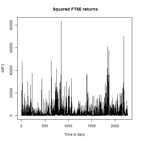
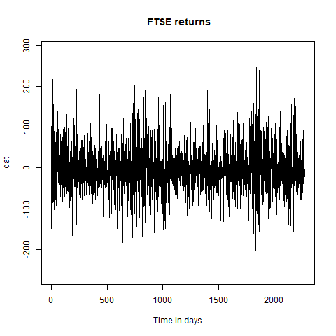
We consider the returns of the daily closing prices of the FTSE index of the London Stock Exchange 100. They are 2273 observations from January 4th, 2010 to December 31st, 2018. The mean and standard deviation of the returns are -0.54 and 57.67, respectively. The Time plot and the correlograns for the log returns and squared log returns are plotted in Figure 1.

The Figures (1(a)) and (1(c)) exhibit the conditional heteroskedasticity in the log return time series. Moreover, Figure (1(b)) shows that more than 5 per cent of the autocorrelations are out of the confidence interval $\pm 1.96/\sqrt{2273}$ and specially the Figure (1(d)) suggests that the strong white noise assumption cannot be sustained for this log-returns sequence of FTSE index.

Refer to caption — (a) Time plot of log returns.

Therefore, the $GARCH(p,q)$ family was considered for the modelling of the FTSE index with $(p,q)\in\llbracket 1;10\rrbracket\times\llbracket 0;10\rrbracket$ which lead us to 110 candidate models. The penalization $\log n$ and $\sqrt{n}$ have been applied to identify the best order and the goodness-of-fit of the selected model has been tested by the portmanteau test. Based on the results of the simulations, we set $K=3$ for the portmanteau test statistic.

The GARCH $(1,1)$ is the ”best” model according to both criteria (related to above penalizations) and the portmanteau statistic $\widehat{Q}_{3}(\widehat{m})\simeq 2.13$ is associated with a p-value of $0.55$ . Hence, the selected model GARCH $(1,1)$ is adequate to model the FTSE 100 index using either criterion.

7 Proofs

We start with the proof of the Proposition 1.

Proof.

For ease of writing, consider only the general case where $f^{(i)}_{\theta_{i}}=g^{(i)}_{\alpha_{i}}$ and $M^{(i)}_{\theta_{i}}=N^{(i)}_{\beta_{i}}$ where $\theta_{i}={}^{t}(\alpha_{i},\beta_{i})$ for $i=1,2$ . Now, assume that there exist $\alpha\in\mathbb{R}^{\delta}$ , where $0\leq\delta\leq\min(d_{1},d_{2})$ and a function $h_{\alpha}$ such as $g^{(1)}_{\alpha_{1}}=h_{\alpha}+\ell^{(1)}_{\alpha^{\prime}_{1}}$ , $f^{(2)}_{\alpha_{2}}=h_{\alpha}+\ell^{(2)}_{\alpha^{\prime}_{2}}$ with $\alpha_{1}={}^{t}(\alpha,\alpha^{\prime}_{1})$ and $\alpha_{2}={}^{t}(\alpha,\alpha^{\prime}_{2})$ and $\ell^{(i)}_{0}=0$ .
Similarly, assume that there exist $\beta\in\mathbb{R}^{\delta^{\prime}}$ , where $0\leq\delta^{\prime}\leq\min(d_{1},d_{2})$ and a function $R_{\beta}$ such as $N^{(1)}_{\beta_{1}}=R_{\beta}+m^{(1)}_{\beta^{\prime}_{1}}$ , $N^{(2)}_{\beta_{2}}=R_{\beta}+m^{(2)}_{\beta_{2}^{\prime}}$ with $\beta_{1}={}^{t}(\beta,\beta^{\prime}_{1})$ and $\beta_{2}={}^{t}(\beta,\beta^{\prime}_{2})$ and $m^{(i)}_{0}=0$ .
Consider now $\theta={}^{t}(\alpha,\alpha^{\prime}_{1},\alpha^{\prime}_{2},\beta,\beta^{\prime}_{1},\beta^{\prime}_{2})\in\mathbb{R}^{d}$ (and therefore $\max(d_{1},d_{2})\leq d\leq d_{1}+d_{2}$ ), $f_{\theta}=h_{\alpha}+\ell^{(1)}_{\alpha^{\prime}_{1}}+\ell^{(2)}_{\alpha^{\prime}_{2}}$ and $M_{\theta}=R_{\beta}+m^{(1)}_{\beta^{\prime}_{1}}+m^{(2)}_{\beta^{\prime}_{2}}$ . Then if $X\in\mathcal{AC}\big(M_{\theta},f_{\theta}\big)$ , for any $t\in\mathbb{Z}$ ,

X_{t}=\big(R_{\beta}((X_{t-k})_{k\geq 1})+m^{(1)}_{\beta^{\prime}_{1}}((X_{t-k})_{k\geq 1})+m^{(2)}_{\beta^{\prime}_{2}}((X_{t-k})_{k\geq 1})\big)\,\xi_{t}\\ +\big(h_{\alpha}((X_{t-k})_{k\geq 1})+\ell^{(1)}_{\alpha^{\prime}_{1}}((X_{t-k})_{k\geq 1})+\ell^{(2)}_{\alpha^{\prime}_{2}}((X_{t-k})_{k\geq 1})\big).

Then, for $\alpha_{2}^{\prime}=\beta_{2}^{\prime}=0$ , $X\in\mathcal{AC}\big(M^{(1)}_{\theta_{1}},f^{(1)}_{\theta_{1}}\big)$ and for $\alpha_{1}^{\prime}=\beta_{1}^{\prime}=0$ , $X\in\mathcal{AC}\big(M^{(2)}_{\theta_{2}},f^{(2)}_{\theta_{2}}\big)$ .
∎

In the sequel, some lemmas are stated and theirs proofs are given.

Lemma 1.

Let $X\in\mathcal{AC}(M_{\theta},f_{\theta})$ (or $\widetilde{\mathcal{AC}}(\widetilde{H}_{\theta})$ ) and $\Theta\subseteq\Theta(r)$ (or $\Theta\subseteq\widetilde{\Theta}(r)$ ) with $r\geq 2$ . Assume that the assumptions $D(\Theta)$ and $K(\Theta)$ (or $\widetilde{K}(\Theta)$ ) hold. Then:

\frac{1}{\kappa_{n}}\,\big\|\widehat{L}_{n}(\theta)-L_{n}(\theta)\big\|_{\Theta}\begin{array}[t]{c}\stackrel{{\scriptstyle a.s.}}{{\longrightarrow}}\\ {\scriptstyle n\rightarrow+\infty}\end{array}0.

(7.1)

Proof.

We have $|\widehat{L}_{n}(\theta)-L_{n}(\theta)|\leq\sum_{t=1}^{n}|\widehat{q}_{t}(\theta)-q_{t}(\theta)|$ . Then,

\frac{1}{\kappa_{n}}\,\big\|\widehat{L}_{n}(\theta)-L_{n}(\theta)\big\|_{\Theta}\leq\frac{1}{\kappa_{n}}\,\sum_{t=1}^{n}\|\widehat{q}_{t}(\theta)-q_{t}(\theta)\|_{\Theta}.

By Corollary 1 of [27], with $r\leq 3$ , (7.1) is established when:

\sum_{k\geq 1}(\frac{1}{\kappa_{k}})^{r/3}\mathbb{E}\big(\|\widehat{q}_{k}(\theta)-q_{k}(\theta)\|_{\Theta}^{r/3}\big)<\infty.

(7.2)

With $r\geq 3$ , and under the assumptions, we first recall some results already obtained in [7]: for any $t\in\mathbb{Z}$ ,

	$\displaystyle\bullet\quad\mathbb{E}\big[\|X_{t}\|^{r}+\\|f_{\theta}^{t}\\|^{r}_{\Theta}+\\|\widehat{f}_{\theta}^{t}\\|^{r}_{\Theta}+\\|M_{\theta}^{t}\\|^{r}_{\Theta}+\\|\widehat{M}_{\theta}^{t}\\|^{r}_{\Theta}+\\|H_{\theta}^{t}\\|^{r/2}_{\Theta}+\\|\widehat{H}_{\theta}^{t}\\|^{r/2}_{\Theta}\big]<\infty$		(7.3)
	$\displaystyle\bullet\quad\left\{\begin{array}[]{l}\mathbb{E}\big[\\|f_{\theta}^{t}-\widehat{f}_{\theta}^{t}\\|^{r}_{\Theta}\big]\leq C\,\Big(\sum_{j\geq t}\alpha_{j}(f_{\theta},\Theta)\Big)^{r}\\ \mathbb{E}\big[\\|M_{\theta}^{t}-\widehat{M}_{\theta}^{t}\\|^{r}_{\Theta}\big]\leq C\,\Big(\sum_{j\geq t}\alpha_{j}(M_{\theta},\Theta)\Big)^{r}\\ \mathbb{E}\big[\\|H_{\theta}^{t}-\widehat{H}_{\theta}^{t}\\|^{r/2}_{\Theta}\big]\leq C\,\Big(\min\Big\{\sum_{j\geq t}\alpha_{j}(M_{\theta},\Theta)\penalty\ ,\penalty\ \sum_{j\geq t}\alpha_{j}(H_{\theta},\Theta)\Big\}\Big)^{r/2}.\end{array}\right.$

For any $\theta\in\Theta$ , we have:

		$\displaystyle\|\widehat{q}_{t}(\theta)-q_{t}(\theta)\|=\Big\|\frac{(X_{t}-\widehat{f}_{\theta}^{t})^{2}}{\widehat{H}_{\theta}^{t}}+\log(\widehat{H}_{\theta}^{t})-\frac{(X_{t}-f_{\theta}^{t})^{2}}{H_{\theta}^{t}}-\log(H_{\theta}^{t})\Big\|$
		$\displaystyle\leq(H_{\theta}^{t}\widehat{H}_{\theta}^{t})^{-1}\big\|H_{\theta}^{t}(X_{t}-\widehat{f}_{\theta}^{t})^{2}-\widehat{H}_{\theta}^{t}(X_{t}-f_{\theta}^{t})^{2}\big\|+\big\|\log(\widehat{H}_{\theta}^{t})-\log(H_{\theta}^{t})\big\|$
		$\displaystyle\leq(H_{\theta}^{t}\widehat{H}_{\theta}^{t})^{-1}\big\|(H_{\theta}^{t}-\widehat{H}_{\theta}^{t})(X_{t}-f_{\theta}^{t})^{2}-H_{\theta}^{t}(X_{t}-f_{\theta}^{t})^{2}+H_{\theta}^{t}(X_{t}-\widehat{f}_{\theta}^{t})^{2}\big\|+\big\|\log(\widehat{H}_{\theta}^{t})-\log(H_{\theta}^{t})\big\|$
		$\displaystyle\leq\underline{h}^{-3/2}\big(\|X_{t}\|^{2}+2\|X_{t}\\|f_{\theta}^{t}\|+\|f_{\theta}^{t}\|^{2}\big)\,\big\|M_{\theta}^{t}-\widehat{M}_{\theta}^{t}\big\|+\underline{h}^{-1}\big(2\|X_{t}\|+\|f_{\theta}^{t}\|+\|\widehat{f}_{\theta}^{t}\|\big)\,\big\|f_{\theta}^{t}-\widehat{f}_{\theta}^{t}\big\|+2\,\big\|\log(\widehat{M}_{\theta}^{t})-\log(M_{\theta}^{t})\big\|$
		$\displaystyle\leq\underline{h}^{-3/2}\big(\|X_{t}\|^{2}+2\|X_{t}\|\times\\|f_{\theta}^{t}\\|_{\Theta}+\\|f_{\theta}^{t}\\|_{\Theta}^{2}\big)\,\\|M_{\theta}^{t}-\widehat{M}_{\theta}^{t}\\|_{\Theta}$
		$\displaystyle\hskip 142.26378pt+\underline{h}^{-1}\big(2\|X_{t}\|+\\|f_{\theta}^{t}\\|_{\Theta}+\\|\widehat{f}_{\theta}^{t}\\|_{\Theta}\big)\,\\|f_{\theta}^{t}-\widehat{f}_{\theta}^{t}\\|_{\Theta}+2\,\underline{h}^{-1/2}\\|\widehat{M}_{\theta}^{t}-M_{\theta}^{t}\\|_{\Theta}.$

1/ If $X\subset{\mathcal{A}C}(M_{\theta},f_{\theta})$ , we deduce

\mathbb{E}\big[\|\widehat{q}_{t}(\theta)-q_{t}(\theta)\|_{\Theta}^{r/3}\big]\leq C\,\Big(\mathbb{E}\Big[\big(\|X_{t}+f_{\theta}^{t}\|_{\Theta}^{2}+1\big)^{r/3}\,\|M_{\theta}^{t}-\widehat{M}_{\theta}^{t}\|^{r/3}_{\Theta}\Big]\\ +\mathbb{E}\Big[\big(2|X_{t}|+\|f_{\theta}^{t}\|_{\Theta}+\|\widehat{f}_{\theta}^{t}\|_{\Theta}\big)^{r/3}\,\|f_{\theta}^{t}-\widehat{f}_{\theta}^{t}\|^{r/3}_{\Theta}\Big]\Big).

(7.8)

Then, by Hölder’s inequality and (7.3) we have:

\mathbb{E}\Big[\big(\|X_{t}+f_{\theta}^{t}\|_{\Theta}^{2}+1\big)^{r/3}\,\|M_{\theta}^{t}-\widehat{M}_{\theta}^{t}\|^{r/3}_{\Theta}\Big]\\ \leq\Big(\mathbb{E}\big[\|X_{t}+f_{\theta}^{t}+1\|_{\Theta}^{r}\big]\Big)^{2/3}\,\Big(\mathbb{E}\big[\|M_{\theta}^{t}-\widehat{M}_{\theta}^{t}\|_{\Theta}^{r}\big]\Big)^{1/3}\leq C\ \Big(\mathbb{E}\big[\|M_{\theta}^{t}-\widehat{M}_{\theta}^{t}\|_{\Theta}^{r}\Big]\Big)^{1/3}.

(7.9)

Again with Hölder’s inequality and (7.3) ,

\mathbb{E}\big[\big((2|X_{t}|+\|f_{\theta}^{t}\|_{\Theta}+\|\widehat{f}_{\theta}^{t}\|_{\Theta})\|f_{\theta}^{t}-\widehat{f}_{\theta}^{t}\|_{\Theta}\big)^{r/3}\big]\leq C\,\big(\mathbb{E}\big[\|f_{\theta}^{t}-\widehat{f}_{\theta}^{t}\|_{\Theta}^{r}]\big)^{1/3}.

(7.10)

Therefore, from (7.9), (7.10) and (7), there exists a constant $C$ such that

\mathbb{E}\big[\|(\widehat{q}_{t}(\theta)-q_{t}(\theta)\|_{\Theta}^{r/3}\big]\leq C\,\Big(\sum_{j\geq t}\alpha_{j}(f_{\theta},\Theta)+\sum_{j\geq t}\alpha_{j}(M_{\theta},\Theta)\Big)^{r/3}.

(7.11)

Hence,

\sum_{k\geq 1}(\frac{1}{\kappa_{k}})^{r/3}\mathbb{E}\big[\|\widehat{q}_{k}(\theta)-q_{k}(\theta)\|_{\Theta}^{r/3}\big]\leq C\,\sum_{k\geq 1}(\frac{1}{\kappa_{k}})^{r/3}\Big(\sum_{j\geq k}\alpha_{j}(f_{\theta},\Theta)+\alpha_{j}(M_{\theta},\Theta)\Big)^{r/3},

which is finite by assumption $K(\Theta)$ , and this achieves the proof.

2/ If $X\subset\widetilde{{\mathcal{A}C}}(\widetilde{H}_{\theta})$ and using Corollary 1 of [27], with $r\leq 4$ , (7.1) is established when:

\sum_{k\geq 1}(\frac{1}{\kappa_{k}})^{r/4}\mathbb{E}\big(\|\widehat{q}_{k}(\theta)-q_{k}(\theta)\|_{\Theta}^{r/4}\big)<\infty.

(7.12)

By proceeding as in the previous case, we deduce

|\widehat{q}_{t}(\theta)-q_{t}(\theta)|\leq\underline{h}^{-2}|X_{t}|^{2}\,\|H_{\theta}^{t}-\widehat{H}_{\theta}^{t}\|_{\Theta}+\underline{h}^{-1}\|\widehat{H}_{\theta}^{t}-H_{\theta}^{t}\|_{\Theta}.

In addition, we deduce that there exists a constant $C$ such that

\mathbb{E}\big[\|(\widehat{q}_{t}(\theta)-q_{t}(\theta)\|_{\Theta}^{r/4}\big]\leq C\,\Big(\sum_{j\geq t}\alpha_{j}(H_{\theta},\Theta)\Big)^{r/4}.

(7.13)

∎

Lemma 2.

\frac{1}{\kappa_{n}}\,\Big\|\dfrac{\partial\widehat{L}_{n}(\theta)}{\partial\theta}-\frac{\partial L_{n}(\theta)}{\partial\theta}\Big\|_{\Theta}\begin{array}[t]{c}\stackrel{{\scriptstyle a.s.}}{{\longrightarrow}}\\ {\scriptstyle n\rightarrow+\infty}\end{array}0.

(7.14)

Proof.

We will go along similar lines as in the proof of Lemma 7.1. We have:

\frac{1}{\kappa_{n}}\,\Big\|\dfrac{\partial\widehat{L}_{n}(\theta)}{\partial\theta}-\frac{\partial L_{n}(\theta)}{\partial\theta}\Big\|_{\Theta}\leq\frac{1}{\kappa_{n}}\,\sum_{t=1}^{n}\Big\|\dfrac{\partial\widehat{q}_{t}(\theta)}{\partial\theta_{i}}-\frac{\partial q_{t}(\theta)}{\partial\theta_{i}}\Big\|_{\Theta}.

Using again Corollary 1 of [27], it is sufficient to prove for $r\leq 3$ that

\sum_{k\geq 1}(\frac{1}{\kappa_{k}})^{r/3}\,\mathbb{E}\Big[\Big\|\dfrac{\partial\widehat{q}_{t}(\theta)}{\partial\theta_{i}}-\frac{\partial q_{t}(\theta)}{\partial\theta_{i}}\Big\|_{\Theta}^{r/3}\Big]<\infty.

(7.15)

For any $\theta\in\Theta$ , with $H_{\theta}=M_{\theta}^{2}$ , the first partial derivatives of $q_{t}(\theta)$ are

\frac{\partial q_{t}(\theta)}{\partial\theta_{i}}=\frac{-2(X_{t}-f_{\theta}^{t})}{H_{\theta}^{t}}\frac{\partial f_{\theta}^{t}}{\partial\theta_{i}}-\frac{(X_{t}-f_{\theta}^{t})^{2}}{(H_{\theta}^{t})^{2}}\frac{\partial H_{\theta}^{t}}{\partial\theta_{i}}+\frac{1}{H_{\theta}^{t}}\frac{\partial H_{\theta}^{t}}{\partial\theta_{i}}\\ =-2(H_{\theta}^{t})^{-1}(X_{t}-f_{\theta}^{t})\frac{\partial f_{\theta}^{t}}{\partial\theta_{i}}+(X_{t}-f_{\theta}^{t})^{2}\frac{\partial(H_{\theta}^{t})^{-1}}{\partial\theta_{i}}+(H_{\theta}^{t})^{-1}\frac{\partial H_{\theta}^{t}}{\partial\theta_{i}},

for $i=1,\cdots,d$ . Hence,

\Big|\frac{\partial\widehat{q}_{t}(\theta)}{\partial\theta_{i}}-\frac{\partial q_{t}(\theta)}{\partial\theta_{i}}\Big|\leq 2\,\Big|(h_{\theta}^{t})^{-1}(X_{t}-f_{\theta}^{t})\frac{\partial f_{\theta}^{t}}{\partial\theta_{i}}-(\widehat{h}_{\theta}^{t})^{-1}(X_{t}-\widehat{f}_{\theta}^{t})\frac{\partial\widehat{f}_{\theta}^{t}}{\partial\theta_{i}}\Big|\\ +\Big|(X_{t}-\widehat{f}_{\theta}^{t})^{2}\frac{\partial(\widehat{H}_{\theta}^{t})^{-1}}{\partial\theta_{i}}-(X_{t}-f_{\theta}^{t})^{2}\frac{\partial(H_{\theta}^{t})^{-1}}{\partial\theta_{i}}\Big|+\Big|(\widehat{H}_{\theta}^{t})^{-1}\frac{\partial\widehat{H}_{\theta}^{t}}{\partial\theta_{i}}-(H_{\theta}^{t})^{-1}\frac{\partial H_{\theta}^{t}}{\partial\theta_{i}}\Big|.

Then, using $|a_{1}b_{1}c_{1}-a_{2}b_{2}c_{2}|\leq|a_{1}-a_{2}|\,|b_{2}|\,|c_{2}|+|a_{1}|\,|b_{1}-b_{2}|\,|c_{2}|+|a_{1}|\,|b_{1}|\,|c_{1}-c_{2}|$ for any $a_{1},a_{2},b_{1},b_{2},c_{1},c_{2}$ in $\mathbb{R}$ , we obtain

	$\displaystyle\Big\|\frac{\partial\widehat{q}_{t}(\theta)}{\partial\theta_{i}}-\frac{\partial q_{t}(\theta)}{\partial\theta_{i}}\Big\|$	$\displaystyle\leq 2\,\Big(\big\|(H_{\theta}^{t})^{-1}-(\widehat{H}_{\theta}^{t})^{-1}\big\|\times\big\|X_{t}-\widehat{f}_{\theta}^{t}\big\|\,\Big\|\frac{\partial\widehat{f}_{\theta}^{t}}{\partial\theta_{i}}\Big\|+\big\|(H_{\theta}^{t})^{-1}\big\|\times\big\|\widehat{f}_{\theta}^{t}-f_{\theta}^{t}\big\|\,\Big\|\frac{\partial\widehat{f}_{\theta}^{t}}{\partial\theta_{i}}\Big\|$
		$\displaystyle+\big\|(H_{\theta}^{t})^{-1}\big\|\times\big\|X_{t}-f_{\theta}^{t}\big\|\,\Big\|\frac{\partial f_{\theta}^{t}}{\partial\theta_{i}}-\frac{\partial\widehat{f}_{\theta}^{t}}{\partial\theta_{i}}\Big\|\Big)+\big\|X_{t}-\widehat{f}_{\theta}^{t}\big\|^{2}\,\Big\|\frac{\partial(\widehat{H}_{\theta}^{t})^{-1}}{\partial\theta_{i}}-\frac{\partial(H_{\theta}^{t})^{-1}}{\partial\theta_{i}}\Big\|$
		$\displaystyle+2\,\Big\|\frac{\partial(H_{\theta}^{t})^{-1}}{\partial\theta_{i}}\Big\|\,\big\|X_{t}\big\|\,\big\|f_{\theta}^{t}-\widehat{f}_{\theta}^{t}\big\|+\big\|(\widehat{H}_{\theta}^{t})^{-1}\big\|\,\Big\|\frac{\partial\widehat{H}_{\theta}^{t}}{\partial\theta_{i}}-\frac{\partial H_{\theta}^{t}}{\partial\theta_{i}}\Big\|+\Big\|\frac{\partial H_{\theta}^{t}}{\partial\theta_{i}}\Big\|\,\big\|(\widehat{H}_{\theta}^{t})^{-1}-(H_{\theta}^{t})^{-1}\big\|.$

Thus,

		$\displaystyle\Big\\|\dfrac{\partial\widehat{q}_{t}(\theta)}{\partial\theta_{i}}-\frac{\partial q_{t}(\theta)}{\partial\theta_{i}}\Big\\|_{\Theta}\leq 2\,\underline{h}^{-1}\Big(\big\\|\widehat{f}_{\theta}^{t}-f_{\theta}^{t}\big\\|_{\Theta}\Big\\|\dfrac{\partial\widehat{f}_{\theta}^{t}}{\partial\theta_{i}}\Big\\|_{\Theta}+\big\\|X_{t}-f_{\theta}^{t}\big\\|_{\Theta}\Big\\|\dfrac{\partial f_{\theta}^{t}}{\partial\theta_{i}}-\frac{\partial\widehat{f}_{\theta}^{t}}{\partial\theta_{i}}\Big\\|_{\Theta}\Big)$
		$\displaystyle\hskip 14.22636pt+2\,\big\\|(H_{\theta}^{t})^{-1}-(\widehat{H}_{\theta}^{t})^{-1}\big\\|_{\Theta}\big\\|X_{t}-\widehat{f}_{\theta}^{t}\big\\|_{\Theta}\Big\\|\dfrac{\partial\widehat{f}_{\theta}^{t}}{\partial\theta_{i}}\Big\\|_{\Theta}+\big\\|X_{t}-\widehat{f}_{\theta}^{t}\big\\|^{2}\Big\\|\dfrac{\partial(\widehat{H}_{\theta}^{t})^{-1}}{\partial\theta_{i}}-\frac{\partial(H_{\theta}^{t})^{-1}}{\partial\theta_{i}}\Big\\|$
		$\displaystyle\hskip 14.22636pt+2\,\big\|X_{t}\big\|\,\big\\|f_{\theta}^{t}-\widehat{f}_{\theta}^{t}\big\\|_{\Theta}\Big\\|\frac{\partial(H_{\theta}^{t})^{-1}}{\partial\theta_{i}}\Big\\|_{\Theta}+\big\\|(\widehat{H}_{\theta}^{t})^{-1}\big\\|_{\Theta}\Big\\|\dfrac{\partial\widehat{H}_{\theta}^{t}}{\partial\theta_{i}}-\frac{\partial H_{\theta}^{t}}{\partial\theta_{i}}\Big\\|_{\Theta}+\big\\|(\widehat{H}_{\theta}^{t})^{-1}-(H_{\theta}^{t})^{-1}\\|_{\Theta}\Big\\|\frac{\partial H_{\theta}^{t}}{\partial\theta_{i}}\Big\\|_{\Theta}.$

Using again the results of [7], we know that:

	$\displaystyle\hskip-42.67912pt\bullet\quad\mathbb{E}\Big[\Big\\|\frac{\partial f_{\theta}^{t}}{\partial\theta_{i}}\Big\\|_{\Theta}^{r}\hskip-5.69054pt+\Big\\|\frac{\partial\widehat{f}_{\theta}^{t}}{\partial\theta_{i}}\Big\\|_{\Theta}^{r}\hskip-5.69054pt+\Big\\|\frac{\partial M_{\theta}^{t}}{\partial\theta_{i}}\Big\\|_{\Theta}^{r}\hskip-5.69054pt+\Big\\|\frac{\partial\widehat{M}_{\theta}^{t}}{\partial\theta_{i}}\Big\\|_{\Theta}^{r}\hskip-5.69054pt+\Big\\|\frac{\partial H_{\theta}^{t}}{\partial\theta_{i}}\Big\\|_{\Theta}^{r/2}\hskip-5.69054pt+\Big\\|\frac{\partial(H_{\theta}^{t})^{-1}}{\partial\theta_{i}}\Big\\|_{\Theta}^{r}\Big]<\infty$		(7.16)
	$\displaystyle\hskip-42.67912pt\bullet\quad\left\{\begin{array}[]{l}\displaystyle\mathbb{E}\big[\big\\|(H_{\theta}^{t})^{-1}-(\widehat{H}_{\theta}^{t})^{-1}\big\\|^{r}_{\Theta}\big]\leq C\,\Big(\sum_{j\geq t}\alpha_{j}(M_{\theta},\Theta)\Big)^{r}\\ \displaystyle\mathbb{E}\Big[\Big\\|\frac{\partial f_{\theta}^{t}}{\partial\theta_{i}}-\frac{\partial\widehat{f}_{\theta}^{t}}{\partial\theta_{i}}\Big\\|^{r}_{\Theta}\Big]\leq C\,\Big(\sum_{j\geq t}\alpha_{j}(\partial f_{\theta},\Theta)\Big)^{r}\\ \displaystyle\mathbb{E}\Big[\Big\\|\frac{\partial H_{\theta}^{t}}{\partial\theta_{i}}-\frac{\partial\widehat{H}_{\theta}^{t}}{\partial\theta_{i}}\Big\\|^{r/2}_{\Theta}\Big]\leq C\,\Big(\sum_{j\geq t}\big(\alpha_{j}(M_{\theta},\Theta)+\alpha_{j}(\partial M_{\theta},\Theta)\big)\Big)^{r/2}\\ \displaystyle\mathbb{E}\Big[\Big\\|\frac{\partial(H_{\theta}^{t})^{-1}}{\partial\theta_{i}}-\frac{\partial(\widehat{H}_{\theta}^{t})^{-1}}{\partial\theta_{i}}\Big\\|^{r/2}_{\Theta}\Big]\leq C\,\Big(\sum_{j\geq t}\big(\alpha_{j}(M_{\theta},\Theta)+\alpha_{j}(\partial M_{\theta},\Theta)\big)\Big)^{r/2}\end{array}\right.$

1. If $X\subset{\mathcal{A}C}(M_{\theta},f_{\theta})$ , we deduce from the Hölder’s Inequality that,

		$\displaystyle\mathbb{E}\Big[\Big\\|\dfrac{\partial\widehat{q}_{t}(\theta)}{\partial\theta_{i}}-\frac{\partial q_{t}(\theta)}{\partial\theta_{i}}\Big\\|_{\Theta}^{r/3}\Big]\leq C\,\Big[\big(\mathbb{E}\big[\big\\|\widehat{f}_{\theta}^{t}-f_{\theta}^{t}\big\\|_{\Theta}^{r}\big]\big)^{1/3}\Big(\mathbb{E}\Big[\Big\\|\dfrac{\partial\widehat{f}_{\theta}^{t}}{\partial\theta_{i}}\Big\\|_{\Theta}^{r/2}\Big]\Big)^{2/3}$
		$\displaystyle+\big(\mathbb{E}\big[\big\\|X_{t}-f_{\theta}^{t}\big\\|_{\Theta}^{2r/3}\big]\big)^{1/2}\Big(\mathbb{E}\Big[\Big\\|\dfrac{\partial f_{\theta}^{t}}{\partial\theta_{i}}-\frac{\partial\widehat{f}_{\theta}^{t}}{\partial\theta_{i}}\Big\\|_{\Theta}^{r}\Big]\Big)^{1/3}$
		$\displaystyle+\big(\mathbb{E}\big[\big\\|(H_{\theta}^{t})^{-1}-(\widehat{H}_{\theta}^{t})^{-1}\big\\|_{\Theta}^{r}\big]\big)^{1/3}\,\Big(\mathbb{E}\big[\big\\|X_{t}-\widehat{f}_{\theta}^{t}\big\\|_{\Theta}^{r}\big]\,\mathbb{E}\Big[\Big\\|\dfrac{\partial\widehat{f}_{\theta}^{t}}{\partial\theta_{i}}\Big\\|_{\Theta}^{r}\Big]\Big)^{1/3}$
		$\displaystyle+\big(\mathbb{E}\big[\big\\|X_{t}-\widehat{f}_{\theta}^{t}\big\\|_{\Theta}^{r}\big]\Big)^{1/3}\Big(\mathbb{E}\Big[\Big\\|\dfrac{\partial(\widehat{H}_{\theta}^{t})^{-1}}{\partial\theta_{i}}-\frac{\partial(H_{\theta}^{t})^{-1}}{\partial\theta_{i}}\Big\\|^{r/2}\Big]\Big)^{2/3}$
		$\displaystyle+\Big(\mathbb{E}\Big[\Big\\|\frac{\partial(H_{\theta}^{t})^{-1}}{\partial\theta_{i}}\Big\\|_{\Theta}^{r}\Big]\Big)^{1/3}\hskip-2.84526pt\Big(\mathbb{E}\big[\|X_{t}\|^{r}\big]\,\mathbb{E}\big[\big\\|f_{\theta}^{t}-\widehat{f}_{\theta}^{t}\big\\|_{\Theta}^{r}\big]\Big)^{1/3}$
		$\displaystyle+\Big(\mathbb{E}\Big[\Big\\|\dfrac{\partial\widehat{H}_{\theta}^{t}}{\partial\theta_{i}}-\frac{\partial H_{\theta}^{t}}{\partial\theta_{i}}\Big\\|_{\Theta}^{r/3}\Big]+\Big(\mathbb{E}\Big[\Big\\|\frac{\partial H_{\theta}^{t}}{\partial\theta_{i}}\Big\\|_{\Theta}^{r/2}\Big]\Big)^{2/3}\big(\mathbb{E}\big[\big\\|(\widehat{H}_{\theta}^{t})^{-1}-(H_{\theta}^{t})^{-1}\big\\|_{\Theta}^{r}\big]\Big)^{1/3}\Big].$

Using (7.16) and (7), we deduce

\mathbb{E}\Big[\Big\|\dfrac{\partial\widehat{q}_{t}(\theta)}{\partial\theta_{i}}-\frac{\partial q_{t}(\theta)}{\partial\theta_{i}}\Big\|_{\Theta}^{r/3}\Big]\leq C\,\Big(\sum_{j\geq t}\alpha_{j}(f_{\theta},\Theta)+\alpha_{j}(M_{\theta},\Theta)+\alpha_{j}(\partial f_{\theta},\Theta)+\alpha_{j}(\partial M_{\theta},\Theta)\Big)^{r/3}.

Therefore,

\sum_{k\geq 1}\frac{1}{\kappa^{r/3}_{k}}\,\mathbb{E}\Big[\Big\|\dfrac{\partial\widehat{q}_{k}(\theta)}{\partial\theta_{i}}-\frac{\partial q_{k}(\theta)}{\partial\theta_{i}}\Big\|_{\Theta}^{r/3}\Big]\\ \leq C\,\sum_{k\geq 1}\frac{1}{\kappa^{r/3}_{k}}\Big(\sum_{j\geq t}\alpha_{j}(f_{\theta},\Theta)+\alpha_{j}(M_{\theta},\Theta)+\alpha_{j}(\partial f_{\theta},\Theta)+\alpha_{j}(\partial M_{\theta},\Theta)\Big)^{r/3}.

We conclude the proof of (7.15) from assumption $K(\Theta)$ .

2. If $X\subset\widetilde{{\mathcal{A}C}}(\widetilde{H}_{\theta})$ , we deduce

\Big\|\dfrac{\partial\widehat{q}_{t}(\theta)}{\partial\theta_{i}}-\frac{\partial q_{t}(\theta)}{\partial\theta_{i}}\Big\|_{\Theta}\leq\big|X_{t}\big|^{2}\,\Big\|\dfrac{\partial(\widehat{H}_{\theta}^{t})^{-1}}{\partial\theta_{i}}-\frac{\partial(H_{\theta}^{t})^{-1}}{\partial\theta_{i}}\Big\|_{\Theta}\\ +\underline{h}^{-1}\Big\|\dfrac{\partial\widehat{H}_{\theta}^{t}}{\partial\theta_{i}}-\frac{\partial H_{\theta}^{t}}{\partial\theta_{i}}\Big\|_{\Theta}+\big\|(\widehat{H}_{\theta}^{t})^{-1}-(H_{\theta}^{t})^{-1}\|_{\Theta}\Big\|\frac{\partial H_{\theta}^{t}}{\partial\theta_{i}}\Big\|_{\Theta}.

As a consequence,

\mathbb{E}\Big[\Big\|\dfrac{\partial\widehat{q}_{t}(\theta)}{\partial\theta_{i}}-\frac{\partial q_{t}(\theta)}{\partial\theta_{i}}\Big\|_{\Theta}^{r/4}\Big]\leq\Big(\mathbb{E}\big[\big|X_{t}\big|^{r}\,\mathbb{E}\Big[\Big\|\dfrac{\partial(\widehat{H}_{\theta}^{t})^{-1}}{\partial\theta_{i}}-\frac{\partial(H_{\theta}^{t})^{-1}}{\partial\theta_{i}}\Big\|^{r/2}_{\Theta}\Big]\Big)^{1/2}\\ +\underline{h}^{-r/4}\mathbb{E}\Big[\Big\|\dfrac{\partial\widehat{H}_{\theta}^{t}}{\partial\theta_{i}}-\frac{\partial H_{\theta}^{t}}{\partial\theta_{i}}\Big\|^{r/4}_{\Theta}\Big]+\Big(\mathbb{E}\big[\big\|(\widehat{H}_{\theta}^{t})^{-1}-(H_{\theta}^{t})^{-1}\|^{r/2}_{\Theta}\big]\,\mathbb{E}\Big[\Big\|\frac{\partial H_{\theta}^{t}}{\partial\theta_{i}}\Big\|^{r/2}_{\Theta}\Big]\Big)^{1/2},

implying

\mathbb{E}\Big[\Big\|\dfrac{\partial\widehat{q}_{t}(\theta)}{\partial\theta_{i}}-\frac{\partial q_{t}(\theta)}{\partial\theta_{i}}\Big\|_{\Theta}^{r/4}\Big]\leq C\,\Big(\sum_{j\geq t}\alpha_{j}(H_{\theta},\Theta)+\alpha_{j}(\partial H_{\theta},\Theta)\Big)^{r/4},

which achieves the proof, according to Corollary 1 of [27]. ∎

Lemma 3.

Under the assumptions of Theorem 3.1 and if a model $m\in\mathcal{M}$ is such that $\theta^{*}\in\Theta(m)$ , then:

\frac{1}{\kappa_{n}}\,\big|\widehat{L}_{n}(\widehat{\theta}(m))-\widehat{L}_{n}(\theta^{*})\big|=o_{P}(1).

(7.22)

Proof.

We have:

	$\displaystyle\frac{1}{\kappa_{n}}\,\big\|\widehat{L}_{n}(\widehat{\theta}(m))-\widehat{L}_{n}(\theta^{*})\big\|$	$\displaystyle=\frac{1}{\kappa_{n}}\,\big\|\widehat{L}_{n}(\widehat{\theta}(m))-L_{n}(\widehat{\theta}(m))+L_{n}(\widehat{\theta}(m))-L_{n}(\theta^{})+L_{n}(\theta^{})-\widehat{L}_{n}(\theta^{*})\big\|$
		$\displaystyle\leq\frac{2}{\kappa_{n}}\,\big\\|\widehat{L}_{n}(\theta)-L_{n}(\theta)\big\\|_{\Theta(r)}+\frac{1}{\kappa_{n}}\,\big\|L_{n}(\widehat{\theta}(m))-L_{n}(\theta^{*})\big\|.$

According to Lemma 7.1, $\frac{1}{\kappa_{n}}\,\big\|\widehat{L}_{n}(\theta)-L_{n}(\theta)\big\|_{\Theta(r)}\begin{array}[t]{c}\stackrel{{\scriptstyle a.s.}}{{\longrightarrow}}\\ {\scriptstyle n\rightarrow+\infty}\end{array}0$ . The proof will be achieved if we prove

\frac{1}{\kappa_{n}}\,\big|L_{n}(\widehat{\theta}(m))-L_{n}(\theta^{*})\big|=o_{P}(1).

(7.23)

Applying a second order Taylor expansion of $L_{n}$ around $\widehat{\theta}(m)$ for $n$ sufficiently large such that $\overline{\theta}(m)\in\Theta(m)$ which are between $\widehat{\theta}(m)$ and $\theta^{*}$ , yields:

\frac{1}{\kappa_{n}}\big(L_{n}(\widehat{\theta}(m))-L_{n}(\theta^{*})\big)=\\ \frac{1}{\kappa_{n}}\big(\widehat{\theta}(m)-\theta^{*}\big)\frac{\partial L_{n}(\widehat{\theta}(m))}{\partial\theta}+\frac{1}{2\kappa_{n}}\big(\widehat{\theta}(m)-\theta^{*}\big)^{\prime}\,\frac{\partial^{2}L_{n}(\overline{\theta}(m))}{\partial\theta^{2}}\,\big(\widehat{\theta}(m)-\theta^{*}\big).\,

(7.24)

Let us deal first with the first term on the right hand side of last equality:

\frac{1}{\kappa_{n}}\,\big(\widehat{\theta}(m)-\theta^{*}\big)\,\frac{\partial L_{n}(\widehat{\theta}(m))}{\partial\theta}=\frac{1}{\kappa_{n}}\,\sqrt{n}\big(\widehat{\theta}(m)-\theta^{*}\big)\,\frac{1}{\sqrt{n}}\,\frac{\partial L_{n}(\widehat{\theta}(m))}{\partial\theta}.

Since $\frac{1}{\kappa_{n}}=o(1)$ and from [7] we have $\sqrt{n}\big(\widehat{\theta}(m)-\theta^{*}\big)=O_{P}(1)$ and $\frac{1}{\sqrt{n}}\,\frac{\partial L_{n}(\widehat{\theta}(m))}{\partial\theta}=o_{P}(1)$ , it follows that:

\frac{1}{\kappa_{n}}\,\big(\widehat{\theta}(m)-\theta^{*}\big)\frac{\partial L_{n}(\widehat{\theta}(m))}{\partial\theta}=o_{P}(1).

(7.25)

On the other hand, for the second term of the right hand side of equality (7.24), let us note that, we have from [7]:

•

$\sqrt{n}\,\big(\widehat{\theta}(m)-\theta^{*}\big)\begin{array}[t]{c}\stackrel{{\scriptstyle{\cal L}}}{{\longrightarrow}}\\ {\scriptstyle n\rightarrow+\infty}\end{array}\mathcal{A}_{\theta^{*},m}$ a Gaussian random variable from (3.2).
•

$\displaystyle-\frac{2}{n}\,\Big(\frac{\partial^{2}L_{n}(\overline{\theta}(m))}{\partial\theta_{i}\partial\theta_{j}}\Big)_{i,j\in m}\begin{array}[t]{c}\stackrel{{\scriptstyle a.s.}}{{\longrightarrow}}\\ {\scriptstyle n\rightarrow+\infty}\end{array}F({\theta}^{*},m)\penalty\$ since $\widehat{\theta}(m)\begin{array}[t]{c}\stackrel{{\scriptstyle a.s.}}{{\longrightarrow}}\\ {\scriptstyle n\rightarrow+\infty}\end{array}\theta^{*}$ and using the assumption Var( $\Theta$ ) insuring that the matrix $F(\theta^{*},m)$ exists and is definite positive (see [7]).

Hence,

\big(\widehat{\theta}(m)-\theta^{*}\big)^{\prime}\,\Big(\frac{\partial^{2}L_{n}(\overline{\theta}(m))}{\partial\theta_{i}\partial\theta_{j}}\Big)_{i,j\in m}(\widehat{\theta}(m)-\theta^{*})\\ =\frac{-1}{2}\sqrt{n}\big(\widehat{\theta}(m)-\theta^{*}\big)^{\prime}\,\big(F(\theta^{*},m)+o_{P}(1)\big)\,\sqrt{n}\big(\widehat{\theta}(m)-\theta^{*}\big)\\ \begin{array}[t]{c}\stackrel{{\scriptstyle{\mathcal{P}}}}{{\longrightarrow}}\\ {\scriptstyle n\rightarrow\infty}\end{array}\frac{-1}{2}\,\mathcal{A}_{\theta^{*},m}^{\prime}\,F(\theta^{*},m)\,\mathcal{A}_{\theta^{*},m}.

We deduce that

\big(\widehat{\theta}(m)-\theta^{*}\big)^{\prime}\,\Big(\frac{\partial^{2}L_{n}(\overline{\theta}(m))}{\partial\theta_{i}\partial\theta_{j}}\Big)_{i,j\in m}(\widehat{\theta}(m)-\theta^{*})=O_{P}(1)\\ \Longrightarrow\quad\frac{1}{\kappa_{n}}\,\big(\widehat{\theta}(m)-\theta^{*}\big)^{\prime}\,\Big(\frac{\partial^{2}L_{n}(\overline{\theta}(m))}{\partial\theta_{i}\partial\theta_{j}}\Big)_{i,j\in m}(\widehat{\theta}(m)-\theta^{*})=o_{P}(1).

(7.26)

Thus, (7.23) follows from (7.24), (7.25) and (7.26); which completes the proof of Lemma 7.22. ∎

7.1 Misspecified model

When a model $m$ is misspecified, we will show that $\mathbb{P}(\widehat{m}=m^{*})\begin{array}[t]{c}\stackrel{{\scriptstyle}}{{\longrightarrow}}\\ {\scriptstyle n\rightarrow\infty}\end{array}0$ following the same scheme of proof than in [42]. Before dealing with this proof, we state some useful results.

Proposition 2.

\Big\|\frac{1}{n}\,L_{n}(\theta)-L(\theta)\Big\|_{\Theta}\begin{array}[t]{c}\stackrel{{\scriptstyle a.s.}}{{\longrightarrow}}\\ {\scriptstyle n\rightarrow+\infty}\end{array}0\quad\mbox{with}\quad L(\theta):=-\frac{1}{2}\,\mathbb{E}[q_{0}(\theta)].

(7.27)

Proof.

See the proof of Theorem 1 in [7]. ∎

Lemma 4.

Under the assumptions of Theorem 3.1 and for $m\in\mathcal{M}$ such as $m^{*}\subset m$ , then:

L_{n}(\widehat{\theta}(m))-L_{n}(\theta^{*})=O_{P}(1).

(7.28)

Proof.

Applying a second order Taylor expansion of $L_{n}$ around $\widehat{\theta}(m^{*})$ for $n$ sufficiently large such that $\overline{\theta}(m)\in\Theta(m)$ which are between $\theta^{*}$ and $\widehat{\theta}(m^{*})$ , yields:

$\displaystyle L_{n}(\widehat{\theta}(m))-L_{n}(\theta^{*})$	$\displaystyle=$	$\displaystyle(\widehat{\theta}(m)-\theta^{})\frac{\partial L_{n}(\widehat{\theta}(m))}{\partial\theta}+\frac{1}{2}(\widehat{\theta}(m)-\theta^{})^{\prime}\frac{\partial^{2}L_{n}(\overline{\theta}(m))}{\partial\theta\partial\theta^{\prime}}(\widehat{\theta}(m)-\theta^{*})$
		$\displaystyle\hskip-56.9055pt=\sqrt{n}(\widehat{\theta}(m)-\theta^{})\frac{1}{\sqrt{n}}\frac{\partial L_{n}(\widehat{\theta}(m))}{\partial\theta}+\frac{1}{2}\sqrt{n}(\widehat{\theta}(m)-\theta^{})^{\prime}\frac{1}{n}\frac{\partial^{2}L_{n}(\overline{\theta}(m))}{\partial\theta\partial\theta^{\prime}}\sqrt{n}(\widehat{\theta}(m)-\theta^{*})$
		$\displaystyle\hskip-56.9055pt=\hskip 42.67912pto_{p}(1)\hskip 85.35826pt+\hskip 42.67912ptO_{P}(1)\hskip 42.67912pt$
		$\displaystyle\hskip-56.9055pt=O_{P}(1),$

by using equality (7.26). ∎

7.2 Proof of Theorem 3.1

As we point out in Subsection 2.4, the proof is divided into two parts.

Proof.

1. For $m\in{\cal M}$ such as $m*\subset m$ and $m\neq m^{*}$ (overfitting), then using with $\widehat{C}(m)=-2\widehat{L}_{n}\big(\widehat{\theta}(m)\big)+|m|\,\kappa_{n}$ (see (2.8)), we have:

$\displaystyle\mathbb{P}(\widehat{m}=m)$	$\displaystyle\leq$	$\displaystyle\mathbb{P}\big(\widehat{C}(m)\leq-2\widehat{L}_{n}\big(\theta^{}\big)+\|m^{}\|\,\kappa_{n}\big)$
	$\displaystyle\leq$	$\displaystyle\mathbb{P}\Big(-2\big(\widehat{L}_{n}(\widehat{\theta})-\widehat{L}_{n}(\theta^{})\big)\leq\kappa_{n}(\|m^{}\|-\|m\|)\Big)$
	$\displaystyle\leq$	$\displaystyle\mathbb{P}\Big(\frac{1}{\kappa_{n}}\big(\widehat{L}_{n}(\theta^{})-\widehat{L}_{n}(\widehat{\theta})\big)\leq\frac{(\|m^{}\|-\|m\|)}{2}\Big)$
	$\displaystyle\begin{array}[t]{c}\stackrel{{\scriptstyle}}{{\longrightarrow}}\\ {\scriptstyle n\rightarrow\infty}\end{array}$	$\displaystyle 0\;$

by virtue of Lemma 7.22 and because $|m|-|m^{*}|\geq 1$ .

2. Let $m\in{\cal M}$ such as $m^{*}\not\subset m$ . Then,

\hskip-14.22636pt\widehat{L}_{n}(\widehat{\theta}(m^{*}))-\widehat{L}_{n}(\widehat{\theta}(m))=\big(\widehat{L}_{n}(\widehat{\theta}(m^{*}))-L_{n}(\widehat{\theta}(m^{*}))\big)-\big(\widehat{L}_{n}(\widehat{\theta}(m))-L_{n}(\widehat{\theta}(m))\big)\\ +\big(L_{n}(\widehat{\theta}(m^{*}))-L_{n}(\widehat{\theta}(m))\big).

(7.30)

It follows from Lemma 7.1 that the first and the second term of the right part of (7.30) are equal to $o_{P}(\kappa_{n})$ . Moreover, the third term can be written as follows:

L_{n}(\widehat{\theta}(m^{*}))-L_{n}(\widehat{\theta}(m))=\big(L_{n}(\widehat{\theta}(m^{*}))-L_{n}(\theta^{*})\big)+\big(L_{n}(\theta^{*})-L_{n}(\widehat{\theta}(m))\big).

From Lemma 4, one deduces $L_{n}(\widehat{\theta}(m^{*}))-L_{n}(\theta^{*})=O_{P}(1)$ . In addition, in the sequel, we are going to show that

L_{n}(\theta^{*})-L_{n}(\widehat{\theta}(m))=n\,\big(A(m)+o_{P}(1)\big),\quad\mbox{with $A(m)>0$}.

(7.31)

For any $\theta\in\Theta(m)$ , we have from Proposition 2

	$\displaystyle L_{n}(\theta^{*})-L_{n}(\theta)$	$\displaystyle=\big(L_{n}(\theta^{})-n\,L(\theta^{})\big)-\big(L_{n}(\theta)-n\,L(\theta)\big)+n\,\big(L(\theta^{*}))-L(\theta))\big)$
		$\displaystyle=o_{P}(n)+n\,\big(L(\theta^{*}))-L(\theta)\big).$

Let us denote by $\mathcal{F}_{t}:=\sigma\big(X_{t-1},X_{t-2},\cdots\big)$ . Using conditional expectation, we obtain

L(\theta^{*})-L(\theta)=-\frac{1}{2}\,\mathbb{E}\Big[\mathbb{E}\big[q_{0}(\theta)-q_{0}(\theta^{*})\penalty\ |\penalty\ \mathcal{F}_{0}\big]\Big].

(7.32)

But,

$\displaystyle\mathbb{E}\big[q_{0}(\theta)-q_{0}(\theta^{*})\penalty\ \|\penalty\ \mathcal{F}_{0}\big]$	$\displaystyle=$	$\displaystyle\mathbb{E}\Big[\frac{(X_{0}-f_{\theta}^{0})^{2}}{H_{\theta}^{0}}+\log(H_{\theta}^{0})-\frac{(X_{0}-f_{\theta^{}}^{0})^{2}}{H_{\theta^{}}^{0}}-\log(H_{\theta^{*}}^{0})\penalty\ \|\penalty\ \mathcal{F}_{0}\Big]$
	$\displaystyle=$	$\displaystyle\log\Big(\frac{H_{\theta}^{0}}{H_{\theta^{}}^{0}}\Big)+\frac{\mathbb{E}\big[(X_{0}-f_{\theta}^{0})^{2}\penalty\ \|\penalty\ \mathcal{F}_{0}\big]}{H_{\theta}^{0}}-\frac{\mathbb{E}\big[(X_{0}-f_{\theta^{}}^{0})^{2}\penalty\ \|\penalty\ \mathcal{F}_{0}\big]}{H_{\theta^{*}}^{0}}$
	$\displaystyle=$	$\displaystyle\log\Big(\frac{H_{\theta}^{0}}{H_{\theta^{}}^{0}}\Big)-1+\frac{\mathbb{E}\big[(X_{0}-f_{\theta^{}}^{0}+f_{\theta^{*}}^{0}-f_{\theta}^{0})^{2}\penalty\ \|\penalty\ \mathcal{F}_{0}\big]}{H_{\theta}^{0}}$
	$\displaystyle=$	$\displaystyle\frac{H_{\theta^{}}^{0}}{H_{\theta}^{0}}-\log\Big(\frac{H_{\theta^{}}^{0}}{H_{\theta}^{0}}\Big)-1+\frac{(f_{\theta^{*}}^{0}-f_{\theta}^{0})^{2}}{H_{\theta}^{0}}$

As a consequence, from (7.32),

$\displaystyle A(m)$	$\displaystyle:=$	$\displaystyle 2\,\big(L(\theta^{*})-L(\theta)\big)$
	$\displaystyle=$	$\displaystyle\mathbb{E}\Big[\frac{H_{\theta^{}}^{0}}{H_{\theta}^{0}}-\log\Big(\frac{H_{\theta^{}}^{0}}{H_{\theta}^{0}}\Big)-1+\frac{(f_{\theta^{*}}^{0}-f_{\theta}^{0})^{2}}{H_{\theta}^{0}}\Big]$
	$\displaystyle\geq$	$\displaystyle\mathbb{E}\Big[\frac{H_{\theta^{}}^{0}}{H_{\theta}^{0}}\Big]-\log\Big(\mathbb{E}\Big[\frac{H_{\theta^{}}^{0}}{H_{\theta}^{0}}\Big]\Big)-1+\mathbb{E}\Big[\frac{(f_{\theta^{*}}^{0}-f_{\theta}^{0})^{2}}{H_{\theta}^{0}}\Big]\quad\mbox{by Jensen Inequality.}$

Since $x-\log(x)-1>0$ for any $x>0,\penalty\ x\neq 1$ and $x-\log(x)-1=0$ for $x=1$ , we deduce that

•

If $f_{\theta^{*}}^{0}\neq f_{\theta}^{0}$ then $\mathbb{E}\Big[\frac{(f_{\theta^{*}}^{0}-f_{\theta}^{0})^{2}}{H_{\theta}^{0}}\Big]>0$ and $A(m)>0.$
•

Otherwise, if $f_{\theta^{*}}^{0}=f_{\theta}^{0}$ , then

$A(m)=\mathbb{E}\Big[\frac{H_{\theta^{*}}^{0}}{H_{\theta}^{0}}-\log\Big(\frac{H_{\theta^{*}}^{0}}{H_{\theta}^{0}}\Big)-1\Big],$

From Assumption ID $(\Theta)$ , when $\theta^{*}\notin\Theta(m)$ and if $f_{\theta^{*}}^{0}=f_{\theta}^{0}$ , we necessarily have $H_{\theta^{*}}^{0}\neq H_{\theta}^{0}$ so that $\frac{H_{\theta^{*}}^{0}}{H_{\theta}^{0}}\neq 1.$ Then $A(m)>0$ .

Therefore $A(m)>0$ for any $\theta\in\Theta(m)$ and particularly for $\theta=\widehat{\theta}(m)$ and (7.31) holds. Thus, (7.30) yields to

\displaystyle\widehat{L}_{n}(\widehat{\theta}(m^{*}))-\widehat{L}_{n}(\widehat{\theta}(m))

\displaystyle=o_{P}(\kappa_{n})+O_{P}(1)+n\,A(m)+o_{P}(n)=O_{P}(1)+n\,A(m)+o_{P}(n).

Finally, when $m\in{\cal M}$ such as $m^{*}\not\subset m$ , we have

\widehat{C}(m)-\widehat{C}(m^{*})=2\,n\,A(m)+o_{P}(n)+O_{P}(1)+\kappa_{n}(|m|-|m^{*}|)\begin{array}[t]{c}\stackrel{{\scriptstyle{\mathcal{P}}}}{{\longrightarrow}}\\ {\scriptstyle n\rightarrow\infty}\end{array}+\infty

since $\kappa_{n}=o(n)$ , therefore $\mathbb{P}\big(\widehat{C}(m)>\widehat{C}(m^{*})\big)\begin{array}[t]{c}\stackrel{{\scriptstyle}}{{\longrightarrow}}\\ {\scriptstyle n\rightarrow\infty}\end{array}1$ .
Thus we have proved the first and most difficult part of Theorem (3.1). The next lines show the second part which is about the consistency of $\widehat{\theta}(\widehat{m})$ .

Given $\epsilon>0$ , we have :

	$\displaystyle\mathbb{P}\Big(\\|\widehat{\theta}(\widehat{m})-\theta^{}\\|_{i\in m^{}}>\epsilon\Big)$	$\displaystyle=$	$\displaystyle\mathbb{P}\Big(\\|\widehat{\theta}(\widehat{m})-\theta^{}\\|_{i\in m^{}}>\epsilon\|\widehat{m}=m^{}\Big)\,\mathbb{P}\big(\widehat{m}=m^{}\big)$
			$\displaystyle\hskip 85.35826pt+\mathbb{P}\Big(\\|\widehat{\theta}(\widehat{m})-\theta^{}\\|_{i\in m^{}}>\epsilon\|\widehat{m}\neq m^{}\Big)\,\mathbb{P}\big(\widehat{m}\neq m^{}\big).$

From the strong consistency of the QMLE (see New version of Theorem 1 of [7]), the first term of the right hand side of the above equation is asymptotically zero and also the second one under the assumptions of the first part of Theorem 3.1 which gives $\mathbb{P}\big(\widehat{m}\neq m^{*}\big)\begin{array}[t]{c}\stackrel{{\scriptstyle}}{{\longrightarrow}}\\ {\scriptstyle n\rightarrow\infty}\end{array}0$ .
∎

7.3 Proof of Theorem 3.2

Proof.

For $x=(x_{i})_{1\leq i\leq d}\in\mathbb{R}^{d}$ , denote $\displaystyle F_{n}(x)=\mathbb{P}\Big(\bigcap_{1\leq i\leq d}\sqrt{n}\,\big(\widehat{\theta}(\widehat{m})-\theta^{*}\big)_{i}\leq x_{i}\Big)$ .
First, we have:

	$\displaystyle F_{n}(x)$	$\displaystyle=$	$\displaystyle\mathbb{P}\Big(\bigcap_{1\leq i\leq d}\sqrt{n}\,\big(\widehat{\theta}(\widehat{m})-\theta^{}\big)_{i}\leq x_{i}\penalty\ \big\|\penalty\ \widehat{m}=m^{}\Big)\,\mathbb{P}\big(\widehat{m}=m^{*}\big)$
			$\displaystyle\hskip 85.35826pt+\mathbb{P}\Big(\bigcap_{1\leq i\leq d}\sqrt{n}\,\big(\widehat{\theta}(\widehat{m})-\theta^{}\big)_{i}\leq x_{i}\penalty\ \big\|\penalty\ \widehat{m}\neq m^{}\Big)\,\mathbb{P}\big(\widehat{m}\neq m^{*}\big).$

Under the assumptions of Theorem 3.1, $\mathbb{P}\big(\widehat{m}=m^{*}\big)\begin{array}[t]{c}\stackrel{{\scriptstyle}}{{\longrightarrow}}\\ {\scriptstyle n\rightarrow\infty}\end{array}1$ and $\mathbb{P}\big(\widehat{m}\neq m^{*}\big)\begin{array}[t]{c}\stackrel{{\scriptstyle}}{{\longrightarrow}}\\ {\scriptstyle n\rightarrow\infty}\end{array}0$ . Therefore the second term in the right side of the previous equality asymptotically vanishes. For the first term, we can write,

\mathbb{P}\Big(\bigcap_{1\leq i\leq d}\sqrt{n}\,\big(\widehat{\theta}(\widehat{m})-\theta^{*}\big)_{i}\leq x_{i}\penalty\ \big|\penalty\ \widehat{m}=m^{*}\Big)\\ =\mathbb{P}\Big(\Big\{\bigcap_{i\in m^{*}}\sqrt{n}\,\big(\widehat{\theta}(m^{*})-\theta^{*}\big)_{i}\leq x_{i}\Big\}\,\bigcap\penalty\ \Big\{\bigcap_{i\notin m^{*}}\sqrt{n}\,\big(\widehat{\theta}(m^{*})-\theta^{*}\big)_{i}\leq x_{i}\Big\}\Big).

Since $\theta(m^{*})\in\Theta(m^{*})$ , $\big(\big(\widehat{\theta}(m^{*})\big)_{i}\big)_{i\notin m^{*}}=\big(\theta^{*}_{i}\big)_{i\notin m^{*}}=0$ , for $(x_{i})_{i\notin m^{*}}$ a family of non negative real numbers we have:

\mathbb{P}\Big(\Big\{\bigcap_{i\in m^{*}}\sqrt{n}\,\big(\widehat{\theta}(m^{*})-\theta^{*}\big)_{i}\leq x_{i}\Big\}\,\bigcap\penalty\ \Big\{\bigcap_{i\notin m^{*}}\sqrt{n}\,\big(\widehat{\theta}(m^{*})-\theta^{*}\big)_{i}\leq x_{i}\Big\}\Big)\\ \hskip-85.35826pt=\mathbb{P}\Big(\bigcap_{i\in m^{*}}\sqrt{n}\,\big(\widehat{\theta}(m^{*})-\theta^{*}\big)_{i}\leq x_{i}\Big)\\ \begin{array}[t]{c}\stackrel{{\scriptstyle}}{{\longrightarrow}}\\ {\scriptstyle n\rightarrow\infty}\end{array}\mathbb{P}\Big(\big(F(\theta^{*},m^{*})^{-1}G(\theta^{*},m^{*})F(\theta^{*},m^{*})^{-1}\big)^{-1/2}Z\leq(x_{i})_{i\in m^{*}}\Big),

with $Z$ a standard Gaussian random vector in $\mathbb{R}^{|m^{*}|}$ from the central limit theorem (3.2), and this achieves the proof of 3.2 of Theorem 3.2. ∎

7.4 Proof of Theorem 5.1

Consider the following notation: for $\theta\in\Theta$ and $m\in{\cal M}$ , denote the residuals and quasi-residuals by:

\left\{\begin{array}[]{lclclcl}e_{t}(\theta)&:=&\displaystyle\big(M_{\theta}^{t}\big)^{-1}\big(X_{t}-f_{\theta}^{t}\big)&\mbox{and}&\widehat{e}_{t}(\theta)&:=&\displaystyle\big(\widehat{M}_{\theta}^{t}\big)^{-1}\big(X_{t}-\widehat{f}_{\theta}^{t}\big)\\ e_{t}(m)&:=&\displaystyle\big(M_{\widehat{\theta}(m)}^{t}\big)^{-1}\big(X_{t}-f_{\widehat{\theta}(m)}^{t}\big)&\mbox{and}&\displaystyle\widehat{e}_{t}(m)&:=&\displaystyle\big(M_{\widehat{\theta}(m)}^{t}\big)^{-1}\big(X_{t}-\widehat{f}_{\widehat{\theta}(m)}^{t}\big)\end{array}\right..

For $k\in\{0,1,\ldots,n-1\}$ , $\theta\in\Theta$ and $m\in{\cal M}$ , define also the adjusted lag- $k$ covariograms and correlograms of the squared (standardized) residual by:

\left\{\begin{array}[]{ccccccc}\gamma_{k}(\theta)&\hskip-8.53581pt:=&\hskip-8.53581pt\displaystyle\frac{1}{n}\,\sum_{t=1}^{n-k}\big(e_{t}^{2}(\theta)-1\big)\big(e_{t+k}^{2}(\theta)-1\big)&\hskip-2.84526pt\mbox{and}&\hskip-2.84526pt\widehat{\gamma}_{k}(\theta)&\hskip-8.53581pt:=&\hskip-8.53581pt\displaystyle\frac{1}{n}\,\sum_{t=1}^{n-k}\big(\widehat{e}_{t}^{2}(\theta)-1\big)\big(\widehat{e}_{t+k}^{2}(\theta)-1\big)\\ \gamma_{k}(m)&\hskip-8.53581pt:=&\hskip-8.53581pt\displaystyle\frac{1}{n}\,\sum_{t=1}^{n-k}\big(e_{t}^{2}(m)-1\big)\big(e_{t+k}^{2}(m)-1\big)&\hskip-2.84526pt\mbox{and}&\hskip-2.84526pt\widehat{\gamma}_{k}(m)&\hskip-8.53581pt:=&\hskip-8.53581pt\displaystyle\frac{1}{n}\,\sum_{t=1}^{n-k}\big(\widehat{e}_{t}^{2}(m)-1\big)\big(\widehat{e}_{t+k}^{2}(m)-1\big)\end{array}\right.

and $\rho_{k}(\theta):=\displaystyle\frac{\gamma_{k}(\theta)}{\gamma_{0}(\theta)},\penalty\ \widehat{\rho}_{k}(\theta):=\displaystyle\frac{\widehat{\gamma}_{k}(\theta)}{\widehat{\gamma}_{0}(\theta)},\penalty\ \rho_{k}(m):=\displaystyle\frac{\gamma_{k}(m)}{\gamma_{0}(m)}$ and $\widehat{\rho}_{k}(m):=\displaystyle\frac{\widehat{\gamma}_{k}(m)}{\widehat{\gamma}_{0}(m)}$ .

Finally, for $K$ a positive integer, denote the vector of adjusted correlogram:

\widehat{\rho}(\theta):=\big(\widehat{\rho}_{1}(\theta),\ldots,\widehat{\rho}_{K}(\theta)\big)^{\prime}\quad\mbox{and}\quad\widehat{\rho}(m):=\big(\widehat{\rho}_{1}(m),\ldots,\widehat{\rho}_{K}(m)\big)^{\prime}.

Proof.

(1) This proof is divided into two parts. In (i) we prove a result that ensures that the asymptotic distributions of the vectors $\widehat{\rho}(\theta)$ and $\rho(\theta)$ are the same. In (ii) we show that the large sample distribution of $\sqrt{n}\rho(m^{*})$ is normal with a covariance matrix $V(\theta^{*},m^{*})$ . Those two conditions do lead well to the asymptotic normality (5.1).

(i) In this part, we first show that for any $k\in\mathbb{N}$ ,

\sqrt{n}\,\big\|\widehat{\gamma}_{k}(\theta)-\gamma_{k}(\theta)\big\|_{\Theta}\begin{array}[t]{c}\stackrel{{\scriptstyle{a.s.}}}{{\longrightarrow}}\\ {\scriptstyle n\rightarrow\infty}\end{array}0.

(7.33)

We have:

$\displaystyle\sqrt{n}\big(\widehat{\gamma}_{k}(\theta)-\gamma_{k}(\theta)\big)$	$\displaystyle=$	$\displaystyle\displaystyle\frac{1}{\sqrt{n}}\,\sum_{t=k+1}^{n}\big(\widehat{e}_{t}^{2}(\theta)-1\big)\big(\widehat{e}_{t-k}^{2}(\theta)-1\big)-\frac{1}{\sqrt{n}}\,\sum_{t=k+1}^{n}\big(e_{t}^{2}(\theta)-1\big)\big(e_{t-k}^{2}(\theta)-1\big)$
	$\displaystyle=$	$\displaystyle\frac{1}{\sqrt{n}}\,\sum_{t=k+1}^{n}\big(\widehat{e}_{t}^{2}(\theta)\widehat{e}_{t-k}^{2}(\theta)-e_{t}^{2}(\theta)e_{t-k}^{2}(\theta)\big)+\frac{1}{\sqrt{n}}\,\sum_{t=k+1}^{n}\big(\widehat{e}_{t}^{2}(\theta)-e_{t}^{2}(\theta)\big)$
		$\displaystyle\hskip 170.71652pt+\frac{1}{\sqrt{n}}\,\sum_{t=k+1}^{n}\big(e_{t-k}^{2}(\theta)-\widehat{e}_{t-k}^{2}(\theta)\big)$
	$\displaystyle=:$	$\displaystyle I_{1}+I_{2}+I_{3}.$

Now, we show that $\|I_{1}\|_{\Theta}\begin{array}[t]{c}\stackrel{{\scriptstyle a.s.}}{{\longrightarrow}}\\ {\scriptstyle n\rightarrow+\infty}\end{array}0$ . We can rewrite $I_{1}$ as follows

	$\displaystyle I_{1}$	$\displaystyle=\frac{1}{\sqrt{n}}\,\sum_{t=k+1}^{n}\widehat{e}_{t-k}^{2}(\theta)\big(\widehat{e}_{t}^{2}(\theta)-e_{t}^{2}(\theta)\big)+\frac{1}{\sqrt{n}}\,\sum_{t=k+1}^{n}e_{t}^{2}(\theta)\big(\widehat{e}_{t-k}^{2}(\theta)-e_{t-k}^{2}(\theta)\big)$
		$\displaystyle=\frac{1}{\sqrt{n}}\,\sum_{t=k+1}^{n}\big(\widehat{e}_{t-k}^{2}(\theta)-e_{t-k}^{2}(\theta)\big)\big(\widehat{e}_{t}^{2}(\theta)-e_{t}^{2}(\theta)\big)+\frac{1}{\sqrt{n}}\,\sum_{t=k+1}^{n}e_{t-k}^{2}(\theta)\big(\widehat{e}_{t}^{2}(\theta)-e_{t}^{2}(\theta)\big)$
		$\displaystyle\hskip 227.62204pt+\frac{1}{\sqrt{n}}\,\sum_{t=k+1}^{n}e_{t}^{2}(\theta)\big(\widehat{e}_{t-k}^{2}(\theta)-e_{t-k}^{2}(\theta)\big)$
		$\displaystyle:=I_{1}^{1}+I_{1}^{2}+I_{1}^{3}.$

Let us show that $\|I_{1}^{1}\|_{\Theta}\begin{array}[t]{c}\stackrel{{\scriptstyle a.s.}}{{\longrightarrow}}\\ {\scriptstyle n\rightarrow+\infty}\end{array}0$ in our two frameworks.
a/ If $X\subset AC(M_{\theta},f_{\theta})$ , by Hölder’s inequality, it follows from (7.11) that,

\displaystyle\mathbb{E}\Big[\Big\|\big(\widehat{e}_{t-k}^{2}(\theta)-e_{t-k}^{2}(\theta)\big)\big(\widehat{e}_{t}^{2}(\theta)-e_{t}^{2}(\theta)\big)\Big\|_{\Theta}^{1/2}\Big]

\displaystyle\leq

\displaystyle\Big(\mathbb{E}\big[\big\|\widehat{e}_{t}^{2}(\theta)-e_{t}^{2}(\theta)\big\|_{\Theta}\big]\times\mathbb{E}\big[\big\|\widehat{e}_{t-k}^{2}(\theta)-e_{t-k}^{2}(\theta)\big\|_{\Theta}\big]\Big)^{1/2}.

But we have

\big\|\widehat{e}_{t}^{2}(\theta)-e_{t}^{2}(\theta)\big\|_{\Theta}\leq\frac{1}{\underline{h}}\,\big(2|X_{t}|+\|\widehat{f}_{\theta}^{t}\|_{\Theta}+\|f_{\theta}^{t}\|_{\Theta}\big)\big\|\widehat{f}_{\theta}^{t}-f_{\theta}^{t}\|_{\Theta}+\frac{4}{\underline{h}^{3/2}}\,\big(|X_{t}|^{2}+\|f_{\theta}^{t}\|^{2}_{\Theta}\big)\big\|\widehat{M}_{\theta}^{t}-M_{\theta}^{t}\|_{\Theta}.

Therefore,

$\displaystyle\mathbb{E}\big[\big\\|\widehat{e}_{t}^{2}(\theta)-e_{t}^{2}(\theta)\big\\|_{\Theta}\big]$	$\displaystyle\leq$	$\displaystyle C\,\Big(\mathbb{E}\big[\big(\|X_{t}\|^{2}+\\|\widehat{f}_{\theta}^{t}\\|^{2}_{\Theta}+\\|f_{\theta}^{t}\\|^{2}_{\Theta}\big)\big]\,\times\,\mathbb{E}\big[\big\\|\widehat{f}_{\theta}^{t}-f_{\theta}^{t}\\|^{2}_{\Theta}\big]\Big)^{1/2}$
		$\displaystyle\hskip 56.9055pt+C\,\Big(\mathbb{E}\big[\big(\|X_{t}\|^{4}+\\|f_{\theta}^{t}\\|^{2}_{\Theta}\big)\big]\,\times\,\mathbb{E}\big[\big\\|\widehat{M}_{\theta}^{t}-M_{\theta}^{t}\\|^{2}_{\Theta}\big]\Big)^{1/2}$
	$\displaystyle\leq$	$\displaystyle C\,\Big(\mathbb{E}\Big[\Big\|\sum_{j\geq t}\alpha_{j}(f_{\theta},\Theta)X_{t-j}\big\|^{2}\Big]\Big)^{1/2}+C\,\Big(\mathbb{E}\Big[\Big\|\sum_{j\geq t}\alpha_{j}(M_{\theta},\Theta)X_{t-j}\big\|^{2}\Big]\Big)^{1/2}$
	$\displaystyle\leq$	$\displaystyle C\,\sum_{j\geq t}\alpha_{j}(f_{\theta},\Theta)+\alpha_{j}(M_{\theta},\Theta),$

using $\mathbb{E}\big[|X_{t}|^{4}+\|f_{\theta}^{t}\|^{2}_{\Theta}+\|\widehat{f}_{\theta}^{t}\|^{2}_{\Theta}\big]<\infty$ and Cauchy-Schwarz Inequality. Hence,

\displaystyle\mathbb{E}\Big[\Big\|\big(\widehat{e}_{t-k}^{2}(\theta)-e_{t-k}^{2}(\theta)\big)\big(\widehat{e}_{t}^{2}(\theta)-e_{t}^{2}(\theta)\big)\Big\|_{\Theta}^{1/2}\Big]

\displaystyle\leq

\displaystyle C\,\sum_{j\geq t-k}\alpha_{j}(f_{\theta},\Theta)+\alpha_{j}(M_{\theta},\Theta).

Therefore, from [27], $\|I^{1}_{1}\|_{\Theta}\begin{array}[t]{c}\stackrel{{\scriptstyle a.s.}}{{\longrightarrow}}\\ {\scriptstyle n\rightarrow+\infty}\end{array}0$ when

\sum_{t=1}^{\infty}t^{-1/4}\sum_{j\geq t}\alpha_{j}(f_{\theta},\Theta)+\alpha_{j}(M_{\theta},\Theta)<\infty.

(7.34)

b/ if $X\subset\widetilde{{\mathcal{A}C}}(\widetilde{H}_{\theta})$ , same computations imply $\|I^{1}_{1}\|_{\Theta}\begin{array}[t]{c}\stackrel{{\scriptstyle a.s.}}{{\longrightarrow}}\\ {\scriptstyle n\rightarrow+\infty}\end{array}0$ when

\sum_{t=1}^{\infty}t^{-1/4}\sum_{j\geq t}\alpha_{j}(\widetilde{H}_{\theta},\Theta)<\infty.

(7.35)

Since $\mathbb{E}\big[\|e_{t}^{2}(\theta)\|_{\Theta}\big]\leq 2\,\underline{h}^{-1}\mathbb{E}\big[X_{t}^{2}+\|f_{\theta}^{t}\|_{\Theta}^{2}\big]<\infty$ and similarly $\mathbb{E}\big[\|\widehat{e}_{t}^{2}(\theta)\|_{\Theta}\big]<\infty$ , we deduce from the same inequalities as in the first case of $I_{1}^{1}$ that $\|I^{2}_{1}\|_{\Theta}\begin{array}[t]{c}\stackrel{{\scriptstyle a.s.}}{{\longrightarrow}}\\ {\scriptstyle n\rightarrow+\infty}\end{array}0$ and $\|I^{3}_{1}\|_{\Theta}\begin{array}[t]{c}\stackrel{{\scriptstyle a.s.}}{{\longrightarrow}}\\ {\scriptstyle n\rightarrow+\infty}\end{array}0$ when

\sum_{t=1}^{\infty}t^{-1/4}\Big(\sum_{j\geq t}\alpha_{j}(f_{\theta},\Theta)+\alpha_{j}(M_{\theta},\Theta)+\alpha_{j}(\widetilde{H}_{\theta},\Theta)\Big)^{1/2}<\infty,

(7.36)

which is also the condition for insuring that $\|I_{2}\|_{\Theta}\begin{array}[t]{c}\stackrel{{\scriptstyle a.s.}}{{\longrightarrow}}\\ {\scriptstyle n\rightarrow+\infty}\end{array}0$ and $\|I_{3}\|_{\Theta}\begin{array}[t]{c}\stackrel{{\scriptstyle a.s.}}{{\longrightarrow}}\\ {\scriptstyle n\rightarrow+\infty}\end{array}0$ . This ends the proof of (7.33).
Finally, since $\widehat{\rho}_{k}(\theta)=\widehat{\gamma}_{k}(\theta)/\widehat{\gamma}_{0}(\theta)$ and $\rho_{k}(\theta)=\gamma_{k}(\theta)/\gamma_{0}(\theta)$ , with $\gamma_{0}(\theta)>0$ , we deduce under condition (7.36) that

\sqrt{n}\big\|\widehat{\rho}_{k}(\theta)-\rho_{k}(\theta)\big\|_{\Theta}\begin{array}[t]{c}\stackrel{{\scriptstyle a.s.}}{{\longrightarrow}}\\ {\scriptstyle n\rightarrow+\infty}\end{array}0\quad\mbox{for any $k\geq 1$}.

(7.37)

This also implies

\sqrt{n}\big|\widehat{\rho}_{k}(m^{*})-\rho_{k}(m^{*})\big|\begin{array}[t]{c}\stackrel{{\scriptstyle a.s.}}{{\longrightarrow}}\\ {\scriptstyle n\rightarrow+\infty}\end{array}0\quad\mbox{for any $k\geq 1$}.

(7.38)

(ii) The proof of this result has already been done in [31] but in a Gaussian framework. We recall here the main lines while avoiding the Gaussian assumption. The first step is to use a Taylor expansion of the function $\gamma$ . Hence, we have for each $k=1,\ldots,K$ ,

\sqrt{n}\,\gamma_{k}(m^{*})=\sqrt{n}\,\gamma_{k}(\widehat{\theta}(m^{*}))=\sqrt{n}\,\gamma_{k}(\theta^{*})+\partial_{\theta}\gamma_{k}(\overline{\theta}^{(k)})\sqrt{n}\,\big((\widehat{\theta}(m^{*}))_{i}-\theta_{i}^{*}\big)_{i\in m^{*}},

(7.39)

where $\partial_{\theta}\gamma_{k}={}^{t}\big(\partial\gamma_{k}/\partial\theta_{i}\big)_{i\in m^{*}}$ , and $\overline{\theta}^{(k)}$ is in the ball of centre $\theta^{*}$ and radius $\|(\widehat{\theta}(m^{*})-\theta^{*})_{i\in m^{*}}\|$ . We also have

\partial_{\theta}\gamma_{k}(\theta)=-\frac{2}{n}\Big(\sum_{t=k+1}^{n}e_{t}^{2}(\theta)\,\big(e_{t-k}^{2}(\theta)-1\big)\frac{\partial_{\theta}M_{\theta}^{t}}{M_{\theta}^{t}}+e_{t}(\theta)\big(e_{t-k}^{2}(\theta)-1\big)\,\frac{\partial_{\theta}f_{\theta}^{t}}{M_{\theta}^{t}}\\ +e_{t-k}(\theta)\,\big(e_{t}^{2}(\theta)-1\big)\frac{\partial_{\theta}f_{\theta}^{t-k}}{M_{\theta}^{t-k}}+e_{t-k}^{2}(\theta)\,\big(e_{t}^{2}(\theta)-1\big)\frac{\partial_{\theta}M_{\theta}^{t-k}}{M_{\theta}^{t-k}}\Big).

(7.40)

We have $\mathbb{E}\big[e_{t-k}(\theta^{*})\,\big(e_{t}^{2}(\theta^{*})-1\big)\frac{\partial f_{\theta^{*}}^{t-k}}{M_{\theta^{*}}^{t-k}}\penalty\ |\penalty\ \sigma\big((\xi_{s})_{s\leq t-k}\big)\big]=e_{t-k}(\theta^{*})\frac{\partial f_{\theta^{*}}^{t-k}}{M_{\theta^{*}}^{t-k}}\mathbb{E}\big[e_{t}^{2}(\theta^{*})-1\big]=0$ since we have assumed $\mathbb{E}[\xi_{0}^{2}]=1$ . Moreover, $\mathbb{E}\big[e_{t}(\theta^{*})\frac{\partial f_{\theta^{*}}^{t}}{M_{\theta^{*}}^{t}}\big]=\mathbb{E}\big[\xi_{t}\,\frac{\partial f_{\theta^{*}}^{t}}{M_{\theta^{*}}^{t}}\big]=0$ and this implies $\mathbb{E}\big[e_{t}(\theta^{*})\big(e_{t-k}^{2}(\theta^{*})-1\big)\,\frac{\partial f_{\theta^{*}}^{t}}{M_{\theta^{*}}^{t}}\big]=0$ . As a consequence, the expectation of the three last terms of (7.40) vanishes for $\theta=\theta^{*}$ . By using the Ergodic Theorem, we finally obtained:

\partial_{\theta}\gamma_{k}(\theta^{*})\begin{array}[t]{c}\stackrel{{\scriptstyle a.s.}}{{\longrightarrow}}\\ {\scriptstyle n\rightarrow+\infty}\end{array}-2\,\mathbb{E}\Big[e_{k}^{2}(\theta^{*})\,\big(e_{0}^{2}(\theta^{*})-1\big)\frac{\partial_{\theta}M_{\theta^{*}}^{k}}{M_{\theta^{*}}^{k}}\Big]=-2\,\mathbb{E}\Big[\big(\xi_{0}^{2}-1\big)\,\partial_{\theta}\log\big(M_{\theta^{*}}^{k}\big)\Big].

Moreover, since $\partial^{2}_{\theta^{2}}f_{\theta}$ and $\partial^{2}_{\theta^{2}}M_{\theta}$ exist, and since $\widehat{\theta}(m^{*})\begin{array}[t]{c}\stackrel{{\scriptstyle a.s.}}{{\longrightarrow}}\\ {\scriptstyle n\rightarrow+\infty}\end{array}\theta^{*}$ , we deduce that the same almost sure convergence occurs for $\partial_{\theta}\gamma_{k}(\overline{\theta}^{(k)})$ . Then, we finally obtain

\big(\partial_{\theta}\gamma_{k}(\overline{\theta}^{(k)})\big)_{1\leq k\leq K}\begin{array}[t]{c}\stackrel{{\scriptstyle a.s.}}{{\longrightarrow}}\\ {\scriptstyle n\rightarrow+\infty}\end{array}J_{K}(m^{*})=-2\,\Big(\mathbb{E}\Big[\big(\xi_{0}^{2}-1\big)\,\frac{\partial}{\partial\theta_{j}}\log\big(M_{\theta^{*}}^{i}\big)\Big]\Big)_{1\leq i\leq K,\,j\in m^{*}}.

(7.41)

We also established a central limit theorem for $\widehat{\theta}(m^{*})$ in (3.2), and this implies

\big(\partial_{\theta}\gamma_{k}(\overline{\theta}^{(k)})\big)_{1\leq k\leq K}\sqrt{n}\,\big((\widehat{\theta}(m^{*}))_{i}-\theta_{i}^{*}\big)_{i\in m^{*}}\\ \begin{array}[t]{c}\stackrel{{\scriptstyle{\cal L}}}{{\longrightarrow}}\\ {\scriptstyle n\rightarrow+\infty}\end{array}{\cal N}_{K}\Big(0\ ,\ J_{K}(m^{*})\,F(\theta^{*},m^{*})^{-1}G(\theta^{*},m^{*})F(\theta^{*},m^{*})^{-1}J^{\prime}_{K}(m^{*})\Big).

(7.42)

On the other hand, when $\theta=\theta^{*}$ , $e^{2}_{t}(\theta^{*})=\xi^{2}_{t}$ for any $t\in\mathbb{Z}$ and since $\mathbb{E}[\xi_{0}^{2}]=1$ , we deduce that $\big(e^{2}_{t}(\theta^{*})-1\big)_{t}$ is a sequence of centred iid random variables with variance $\mu_{4}-1$ with $\mu_{4}=\mathbb{E}[\xi_{0}^{4}]$ . In such as case, the asymptotic behavior of the covariograms is well known and we deduce:

\sqrt{n}\,\big(\gamma_{k}(\theta^{*})\big)_{1\leq k\leq K}\begin{array}[t]{c}\stackrel{{\scriptstyle{\cal L}}}{{\longrightarrow}}\\ {\scriptstyle n\rightarrow+\infty}\end{array}{\cal N}_{K}\big(0\,,\,(\mu_{4}-1)^{2}\,I_{K}\big),

(7.43)

with $I_{k}$ the $(K\times K)$ identity matrix.

We would like to use (7.39) for obtaining the asymptotic behavior of $\gamma(m^{*})$ . In (7.42) and (7.43), we obtained the asymptotic normality of each of the two terms composing $\gamma(m^{*})$ . Now we need to study the joint asymptotic behavior of $\sqrt{n}\,\gamma(\theta^{*})$ and $\sqrt{n}\,\big((\widehat{\theta}(m^{*}))_{i}-\theta_{i}^{*}\big)_{i\in m^{*}}$ .

Using the proof of the asymptotic normality of the QMLE (see for instance [7]), a Taylor expansion of log-likelihood for large $n$ leads to

\big((\widehat{\theta}(m^{*}))_{i}-\theta_{i}^{*}\big)_{i\in m^{*}}\approx-\big(F(\theta^{*},m^{*})\big)^{-1}\frac{1}{n}\,\frac{\partial}{\partial\theta}L_{n}(\theta^{*}).

Therefore, the asymptotic cross expectation between $\big(\partial_{\theta}\gamma_{k}(\overline{\theta}^{(k)})\big)_{k}\sqrt{n}\,\big((\widehat{\theta}(m^{*}))_{i}-\theta_{i}^{*}\big)_{i\in m^{*}}$ and $\sqrt{n}\,\gamma(\theta^{*})$ is equal to:

-\,J_{K}(m^{*})\,F(\theta^{*},m^{*})^{-1}\mathbb{E}\Big[\frac{\partial}{\partial\theta}L_{n}(\theta^{*})\,\gamma(\theta^{*})^{\prime}\Big].

(7.44)

From (2.5), a direct differentiation of $L_{n}$ provides

\frac{\partial}{\partial\theta}L_{n}(\theta^{*})=\sum_{t=1}^{n}\big(e_{t}^{2}(\theta^{*})-1\big)\,\frac{\partial}{\partial\theta}\log\big(M_{\theta^{*}}^{t}\big)+\sum_{t=1}^{n}e_{t}(\theta^{*})\,\frac{\partial}{\partial\theta}f_{\theta^{*}}^{t}

so that,

$\displaystyle\mathbb{E}\Big[\frac{\partial}{\partial\theta}L_{n}(\theta^{})\,\gamma_{k}(\theta^{})\Big]$	$\displaystyle=$	$\displaystyle\frac{1}{n}\,\mathbb{E}\Big[\sum_{i=1}^{n}\big(e_{i}^{2}(\theta^{})-1\big)\,\frac{\partial}{\partial\theta}\log\big(M_{\theta^{}}^{i}\big)\sum_{j=k+1}^{n}\big(e_{j}^{2}(\theta^{})-1\big)\,\big(e_{j-k}^{2}(\theta^{})-1\big)\Big]$
		$\displaystyle\hskip 56.9055pt+\frac{1}{n}\,\mathbb{E}\Big[\sum_{i=1}^{n}e_{i}(\theta^{})\,\frac{\partial}{\partial\theta}f_{\theta^{}}^{i}\sum_{j=k+1}^{n}\big(e_{j}^{2}(\theta^{})-1\big)\,\big(e_{j-k}^{2}(\theta^{})-1\big)\Big]$
	$\displaystyle=$	$\displaystyle\frac{1}{n}\,\sum_{i=1}^{n}\sum_{j=k+1}^{n}\mathbb{E}\Big[\big(\xi_{i}^{2}-1\big)\,\big(\xi_{j}^{2}-1\big)\,\big(\xi_{j-k}^{2}-1\big)\,\frac{\partial}{\partial\theta}\log\big(M_{\theta^{*}}^{i}\big)\Big]$
		$\displaystyle\hskip 56.9055pt+\frac{1}{n}\,\sum_{i=1}^{n}\sum_{j=k+1}^{n}\mathbb{E}\Big[\xi_{i}\,\big(\xi_{j}^{2}-1\big)\,\big(\xi_{j-k}^{2}-1\big)\,\frac{\partial}{\partial\theta}f_{\theta^{*}}^{i}\Big].$

Using conditional expectations, we have $\mathbb{E}\Big[\big(\xi_{i}^{2}-1\big)\,\big(\xi_{j}^{2}-1\big)\,\big(\xi_{j-k}^{2}-1\big)\,\frac{\partial}{\partial\theta}\log\big(M_{\theta^{*}}^{i}\big)\Big]=0$ for $i\neq j$ since $k\geq 1$ . Moreover, for $i=j$ , we obtain:

\mathbb{E}\Big[\big(\xi_{i}^{2}-1\big)\,\big(\xi_{j}^{2}-1\big)\,\big(\xi_{j-k}^{2}-1\big)\,\frac{\partial}{\partial\theta}\log\big(M_{\theta^{*}}^{i}\big)\Big]=(\mu_{4}-1)\,\mathbb{E}\Big[\big(\xi_{i-k}^{2}-1\big)\,\frac{\partial}{\partial\theta}\log\big(M_{\theta^{*}}^{i}\big)\Big],

which is the row $k$ of matrix $-\frac{(\mu_{4}-1)}{2}\,J_{K}(m^{*})$ . Similarly, and using the assumption $\mathbb{E}\big[\xi^{3}_{0}]=0$ , we obtain $\mathbb{E}\Big[\xi_{i}\,\big(\xi_{j}^{2}-1\big)\,\big(\xi_{j-k}^{2}-1\big)\,\frac{\partial}{\partial\theta}f_{\theta^{*}}^{i}\Big]=0$ for any $i,j$ and $k$ . As a consequence,

\mbox{Cov}\,\big(\sqrt{n}\,\gamma(\theta^{*})\,,\,\big(\partial_{\theta}\gamma_{k}(\overline{\theta}^{(k)})\big)_{k}\sqrt{n}\,\big((\widehat{\theta}(m^{*}))_{i}-\theta_{i}^{*}\big)_{i\in m^{*}}\big)\\ \begin{array}[t]{c}\stackrel{{\scriptstyle}}{{\longrightarrow}}\\ {\scriptstyle n\rightarrow\infty}\end{array}\frac{1}{2}\,(\mu_{4}-1)\,J_{K}(m^{*})\,F(\theta^{*},m^{*})^{-1}\,J^{\prime}_{K}(m^{*}).

Finally, we deduce the asymptotic covariance matrix of $\sqrt{n}\,\gamma(m^{*})$ , which is

(\mu_{4}-1)^{2}\,I_{K}+J_{K}(m^{*})\,F(\theta^{*},m^{*})^{-1}G(\theta^{*},m^{*})F(\theta^{*},m^{*})^{-1}J^{\prime}_{K}(m^{*})\\ +(\mu_{4}-1)\,J_{K}(m^{*})\,F(\theta^{*},m^{*})^{-1}\,J^{\prime}_{K}(m^{*}).

Moreover the vector $\gamma(m^{*})$ is normal distributed from Lemma 3.3 of [32].
Thus, using Slutsky Lemma and with $\gamma_{0}(m^{*})\begin{array}[t]{c}\stackrel{{\scriptstyle a.s.}}{{\longrightarrow}}\\ {\scriptstyle n\rightarrow+\infty}\end{array}\mu_{4}-1$ , and with $\rho_{k}(m^{*})=\gamma_{k}(m^{*})/\gamma_{0}(m^{*})$ , the limit theorem (5.1) holds with

V(\theta^{*},m^{*}):=I_{K}+(\mu_{4}-1)^{-2}\,J_{K}(m^{*})\,F(\theta^{*},m^{*})^{-1}G(\theta^{*},m^{*})F(\theta^{*},m^{*})^{-1}J^{\prime}_{K}(m^{*})\\ +(\mu_{4}-1)^{-1}\,J_{K}(m^{*})\,F(\theta^{*},m^{*})^{-1}\,J^{\prime}_{K}(m^{*}).

(7.45)

The proof is achieved after using the limit theorem (7.38).

(2) (5.2) follows directly from (5.1).

(3) We follow a same reasoning like in the proof of Theorem 3.2. For $x=(x_{k})_{1\leq k\leq K}\in\mathbb{R}^{K}$ , denote by $\displaystyle F_{n}(x)=\mathbb{P}\Big(\bigcap_{1\leq k\leq K}\sqrt{n}\,\big(\widehat{\rho}(\widehat{m})\big)_{k}\leq x_{k}\Big)$ the distribution function of $\sqrt{n}\widehat{\rho}(\widehat{m}).$
Applying the Total Probability Rule and by virtue of Theorem 3.1, we obtain:

F_{n}(x)=\mathbb{P}\Big(\bigcap_{1\leq k\leq K}\sqrt{n}\,\big(\widehat{\rho}(m^{*})\big)_{k}\leq x_{k}\Big).

Therefore, the vectors $\sqrt{n}\widehat{\rho}(\widehat{m})$ and $\sqrt{n}\widehat{\rho}(m^{*})$ have exactly the same distribution. ∎

References

[1] Akaike, H. Information theory and an extension of the maximum likelihood principle. Proceedings of the 2nd international symposium on information, Akademiai Kiado, Budapest (1973).
[2] Allen, D. The relationship between variable selection and data agumentation and a method for prediction. Technometrics 16, 1 (1974), 125–127.
[3] Alquier, P., and Wintenberger, O. Model selection for weakly dependent time series forecasting. Bernoulli 18, 3 (2012), 883–913.
[4] Arkoun, O., Brua, J.-Y., and Pergamenshchikov, S. Sequential model selection method for nonparametric autoregression. arXiv preprint arXiv:1809.02241 (2018).
[5] Arlot, S., and Massart, P. Data-driven calibration of penalties for least-squares regression. Journal of Machine learning research 10 (2009), 245–279.
[6] Bardet, J.-M., Boularouk, Y., and Djaballah, K. Asymptotic behavior of the laplacian quasi-maximum likelihood estimator of affine causal processes. Electronic journal of statistics 11, 1 (2017), 452–479.
[7] Bardet, J.-M., and Wintenberger, O. Asymptotic normality of the quasi-maximum likelihood estimator for multidimensional causal processes. The Annals of Statistics 37, 5B (2009), 2730–2759.
[8] Berkes, I., Horváth, L., and Kokoszka, P. GARCH processes: structure and estimation. Bernoulli 9 (2003), 201–227.
[9] Birgé, L., and Massart, P. Minimal penalties for gaussian model selection. Probability theory and related fields 138, 1-2 (2007), 33–73.
[10] Ding, J., Tarokh, V., and Yang, Y. Bridging aic and bic: a new criterion for autoregression. IEEE Transactions on Information Theory 64, 6 (2018), 4024–4043.
[11] Ding, J., Tarokh, V., and Yang, Y. Model selection techniques: An overview. IEEE Signal Processing Magazine 35, 6 (2018), 16–34.
[12] Ding, Z., Granger, C., and Engle, R. A long memory property of stock market returns and a new model. Journal of empirical finance 1, 1 (1993), 83–106.
[13] Doukhan, P., and Wintenberger, O. Weakly dependent chains with infinite memory. Stochastic Processes and their Applications 118, 11 (2008), 1997–2013.
[14] Duchesne, P., and Francq, C. On diagnostic checking time series models with portmanteau test statistics based on generalized inverses and. In COMPSTAT 2008. Springer, 2008, pp. 143–154.
[15] Francq, C., and Zakoïan, J.-M. Maximum likelihood estimation of pure garch and arma-garch processes. Bernoulli 10 (2004), 605–637.
[16] Gao, J., and Tong, H. Semiparametric non-linear time series model selection. Journal of the Royal Statistical Society: Series B 66, 2 (2004), 321–336.
[17] Hannan, E. The estimation of the order of an arma process. The Annals of Statistics 8, 5 (1980), 1071–1081.
[18] Hoerl, A., and Kennard, R. Ridge regression: Biased estimation for nonorthogonal problems. Technometrics 12, 1 (1970), 55–67.
[19] Hsu, H.-L., Ing, C.-K., and Tong, H. On model selection from a finite family of possibly misspecified time series models. The Annals of Statistics 47, 2 (2019), 1061–1087.
[20] Hurvich, C., and Tsai, C.-L. Regression and time series model selection in small samples. Biometrika 76, 2 (1989), 297–307.
[21] Ing, C.-K. Accumulated prediction errors, information criteria and optimal forecasting for autoregressive time series. The Annals of Statistics 35, 3 (2007), 1238–1277.
[22] Ing, C.-K., Sin, C.-Y., and Yu, S.-H. Model selection for integrated autoregressive processes of infinite order. Journal of Multivariate Analysis 106 (2012), 57–71.
[23] Ing, C.-K., and Wei, C.-Z. Order selection for same-realization predictions in autoregressive processes. The Annals of Statistics 33, 5 (2005), 2423–2474.
[24] Jeantheau, T. Strong consistency of estimators for multivariate arch models. Econometric Theory 14, 1 (1998), 70–86.
[25] Kapetanios, G. Model selection in threshold models. Journal of Time Series Analysis 22, 6 (2001), 733–754.
[26] Kock, A. Consistent and conservative model selection with the adaptive lasso in stationary and nonstationary autoregressions. Econometric Theory 32, 1 (2016), 243–259.
[27] Kounias, E., and Weng, T. An inequality and almost sure convergence. The Annals of Mathematical Statistics 40, 3 (1969), 1091–1093.
[28] Lerasle, M. Optimal model selection for density estimation of stationary data under various mixing conditions. The Annals of Statistics 39, 4 (2011), 1852–1877.
[29] Li, G., and Li, W. Least absolute deviation estimation for fractionally integrated autoregressive moving average time series models with conditional heteroscedasticity. Biometrika 95, 2 (2008), 399–414.
[30] Li, W. On the asymptotic standard errors of residual autocorrelations in nonlinear time series modelling. Biometrika 79, 2 (1992), 435–437.
[31] Li, W., and Mak, T. On the squared residual autocorrelations in non-linear time series with conditional heteroskedasticity. Journal of Time Series Analysis 15, 6 (1994), 627–636.
[32] Ling, S., and Li, W.-K. Diagnostic checking of nonlinear multivariate time series with multivariate arch errors. Journal of Time Series Analysis 18, 5 (1997), 447–464.
[33] Ling, S., and McAleer, M. Asymptotic theory for a vector arma-garch model. Econometric theory 19, 2 (2003), 280–310.
[34] Mallows, C. Some comments on cp. Technometrics 15, 4 (1973), 661–675.
[35] McQuarrie, A., and Tsai, C. Regression and Time Series Model Selection. World Scientific Pub Co Inc, 1998.
[36] Rao, C., Wu, Y., Konishi, S., and Mukerjee, R. On model selection. Lecture Notes-Monograph Series (2001), 1–64.
[37] Ren, Y., and Zhang, X. Subset selection for vector autoregressive processes via adaptive lasso. Statistics & probability letters 80, 23-24 (2010), 1705–1712.
[38] Schwarz, G. Estimating the dimension of a model. The annals of statistics 6, 2 (1978), 461–464.
[39] Shao, Q., and Yang, L. Oracally efficient estimation and consistent model selection for auto-regressive moving average time series with trend. Journal of the Royal Statistical Society: Series B 79, 2 (2017), 507–524.
[40] Shi, P., and Tsai, C.-L. Regression model selection-a residual likelihood approach. Journal of the Royal Statistical Society: Series B 64, 2 (2002), 237–252.
[41] Shibata, R. Asymptotically efficient selection of the order of the model for estimating parameters of a linear process. The Annals of Statistics (1980), 147–164.
[42] Sin, C.-Y., and White, H. Information criteria for selecting possibly misspecified parametric models. Journal of Econometrics 71, 1-2 (1996), 207–225.
[43] Stone, M. Cross-validatory choice and assessment of statistical predictions. Journal of the royal statistical society. Series B (1974), 111–147.
[44] Straumann, D., and Mikosch, T. Quasi-maximum-likelihood estimation in conditionally heteroscedastic time series: A stochastic recurrence equations approach. The Annals of Statistics 34, 5 (2006), 2449–2495.
[45] Tibshirani, R. Regression shrinkage and selection via the lasso. Journal of the Royal Statistical Society. Series B (1996), 267–288.
[46] Tsay, R. Order selection in nonstationary autoregressive models. The Annals of Statistics 12, 4 (1984), 1425–1433.
[47] Tse, Y., and Zuo, X. Testing for conditional heteroscedasticity: Some monte carlo results. Journal of Statistical Computation and Simulation 58, 3 (1997), 237–253.
[48] White, H. Maximum likelihood estimation of misspecified models. Econometrica (1982), 1–25.
[49] Zou, H. The adaptive lasso and its oracle properties. Journal of the American Statistical Association 101, 476 (2006), 1418–1429.
[50] Zou, H., and Hastie, T. Regularization and variable selection via the elastic net. Journal of the Royal Statistical Society: Series B 67, 2 (2005), 301–320.

		$\displaystyle\|\widehat{q}_{t}(\theta)-q_{t}(\theta)\|=\Big\|\frac{(X_{t}-\widehat{f}_{\theta}^{t})^{2}}{\widehat{H}_{\theta}^{t}}+\log(\widehat{H}_{\theta}^{t})-\frac{(X_{t}-f_{\theta}^{t})^{2}}{H_{\theta}^{t}}-\log(H_{\theta}^{t})\Big\|$
		$\displaystyle\leq(H_{\theta}^{t}\widehat{H}_{\theta}^{t})^{-1}\big\|H_{\theta}^{t}(X_{t}-\widehat{f}_{\theta}^{t})^{2}-\widehat{H}_{\theta}^{t}(X_{t}-f_{\theta}^{t})^{2}\big\|+\big\|\log(\widehat{H}_{\theta}^{t})-\log(H_{\theta}^{t})\big\|$
		$\displaystyle\leq(H_{\theta}^{t}\widehat{H}_{\theta}^{t})^{-1}\big\|(H_{\theta}^{t}-\widehat{H}_{\theta}^{t})(X_{t}-f_{\theta}^{t})^{2}-H_{\theta}^{t}(X_{t}-f_{\theta}^{t})^{2}+H_{\theta}^{t}(X_{t}-\widehat{f}_{\theta}^{t})^{2}\big\|+\big\|\log(\widehat{H}_{\theta}^{t})-\log(H_{\theta}^{t})\big\|$
		$\displaystyle\leq\underline{h}^{-3/2}\big(\|X_{t}\|^{2}+2\|X_{t}\\|f_{\theta}^{t}\|+\|f_{\theta}^{t}\|^{2}\big)\,\big\|M_{\theta}^{t}-\widehat{M}_{\theta}^{t}\big\|+\underline{h}^{-1}\big(2\|X_{t}\|+\|f_{\theta}^{t}\|+\|\widehat{f}_{\theta}^{t}\|\big)\,\big\|f_{\theta}^{t}-\widehat{f}_{\theta}^{t}\big\|+2\,\big\|\log(\widehat{M}_{\theta}^{t})-\log(M_{\theta}^{t})\big\|$
		$\displaystyle\leq\underline{h}^{-3/2}\big(\|X_{t}\|^{2}+2\|X_{t}\|\times\\|f_{\theta}^{t}\\|_{\Theta}+\\|f_{\theta}^{t}\\|_{\Theta}^{2}\big)\,\\|M_{\theta}^{t}-\widehat{M}_{\theta}^{t}\\|_{\Theta}$
		$\displaystyle\hskip 142.26378pt+\underline{h}^{-1}\big(2\|X_{t}\|+\\|f_{\theta}^{t}\\|_{\Theta}+\\|\widehat{f}_{\theta}^{t}\\|_{\Theta}\big)\,\\|f_{\theta}^{t}-\widehat{f}_{\theta}^{t}\\|_{\Theta}+2\,\underline{h}^{-1/2}\\|\widehat{M}_{\theta}^{t}-M_{\theta}^{t}\\|_{\Theta}.$

	$\displaystyle\Big\|\frac{\partial\widehat{q}_{t}(\theta)}{\partial\theta_{i}}-\frac{\partial q_{t}(\theta)}{\partial\theta_{i}}\Big\|$	$\displaystyle\leq 2\,\Big(\big\|(H_{\theta}^{t})^{-1}-(\widehat{H}_{\theta}^{t})^{-1}\big\|\times\big\|X_{t}-\widehat{f}_{\theta}^{t}\big\|\,\Big\|\frac{\partial\widehat{f}_{\theta}^{t}}{\partial\theta_{i}}\Big\|+\big\|(H_{\theta}^{t})^{-1}\big\|\times\big\|\widehat{f}_{\theta}^{t}-f_{\theta}^{t}\big\|\,\Big\|\frac{\partial\widehat{f}_{\theta}^{t}}{\partial\theta_{i}}\Big\|$
		$\displaystyle+\big\|(H_{\theta}^{t})^{-1}\big\|\times\big\|X_{t}-f_{\theta}^{t}\big\|\,\Big\|\frac{\partial f_{\theta}^{t}}{\partial\theta_{i}}-\frac{\partial\widehat{f}_{\theta}^{t}}{\partial\theta_{i}}\Big\|\Big)+\big\|X_{t}-\widehat{f}_{\theta}^{t}\big\|^{2}\,\Big\|\frac{\partial(\widehat{H}_{\theta}^{t})^{-1}}{\partial\theta_{i}}-\frac{\partial(H_{\theta}^{t})^{-1}}{\partial\theta_{i}}\Big\|$
		$\displaystyle+2\,\Big\|\frac{\partial(H_{\theta}^{t})^{-1}}{\partial\theta_{i}}\Big\|\,\big\|X_{t}\big\|\,\big\|f_{\theta}^{t}-\widehat{f}_{\theta}^{t}\big\|+\big\|(\widehat{H}_{\theta}^{t})^{-1}\big\|\,\Big\|\frac{\partial\widehat{H}_{\theta}^{t}}{\partial\theta_{i}}-\frac{\partial H_{\theta}^{t}}{\partial\theta_{i}}\Big\|+\Big\|\frac{\partial H_{\theta}^{t}}{\partial\theta_{i}}\Big\|\,\big\|(\widehat{H}_{\theta}^{t})^{-1}-(H_{\theta}^{t})^{-1}\big\|.$

		$\displaystyle\mathbb{E}\Big[\Big\\|\dfrac{\partial\widehat{q}_{t}(\theta)}{\partial\theta_{i}}-\frac{\partial q_{t}(\theta)}{\partial\theta_{i}}\Big\\|_{\Theta}^{r/3}\Big]\leq C\,\Big[\big(\mathbb{E}\big[\big\\|\widehat{f}_{\theta}^{t}-f_{\theta}^{t}\big\\|_{\Theta}^{r}\big]\big)^{1/3}\Big(\mathbb{E}\Big[\Big\\|\dfrac{\partial\widehat{f}_{\theta}^{t}}{\partial\theta_{i}}\Big\\|_{\Theta}^{r/2}\Big]\Big)^{2/3}$
		$\displaystyle+\big(\mathbb{E}\big[\big\\|X_{t}-f_{\theta}^{t}\big\\|_{\Theta}^{2r/3}\big]\big)^{1/2}\Big(\mathbb{E}\Big[\Big\\|\dfrac{\partial f_{\theta}^{t}}{\partial\theta_{i}}-\frac{\partial\widehat{f}_{\theta}^{t}}{\partial\theta_{i}}\Big\\|_{\Theta}^{r}\Big]\Big)^{1/3}$
		$\displaystyle+\big(\mathbb{E}\big[\big\\|(H_{\theta}^{t})^{-1}-(\widehat{H}_{\theta}^{t})^{-1}\big\\|_{\Theta}^{r}\big]\big)^{1/3}\,\Big(\mathbb{E}\big[\big\\|X_{t}-\widehat{f}_{\theta}^{t}\big\\|_{\Theta}^{r}\big]\,\mathbb{E}\Big[\Big\\|\dfrac{\partial\widehat{f}_{\theta}^{t}}{\partial\theta_{i}}\Big\\|_{\Theta}^{r}\Big]\Big)^{1/3}$
		$\displaystyle+\big(\mathbb{E}\big[\big\\|X_{t}-\widehat{f}_{\theta}^{t}\big\\|_{\Theta}^{r}\big]\Big)^{1/3}\Big(\mathbb{E}\Big[\Big\\|\dfrac{\partial(\widehat{H}_{\theta}^{t})^{-1}}{\partial\theta_{i}}-\frac{\partial(H_{\theta}^{t})^{-1}}{\partial\theta_{i}}\Big\\|^{r/2}\Big]\Big)^{2/3}$
		$\displaystyle+\Big(\mathbb{E}\Big[\Big\\|\frac{\partial(H_{\theta}^{t})^{-1}}{\partial\theta_{i}}\Big\\|_{\Theta}^{r}\Big]\Big)^{1/3}\hskip-2.84526pt\Big(\mathbb{E}\big[\|X_{t}\|^{r}\big]\,\mathbb{E}\big[\big\\|f_{\theta}^{t}-\widehat{f}_{\theta}^{t}\big\\|_{\Theta}^{r}\big]\Big)^{1/3}$
		$\displaystyle+\Big(\mathbb{E}\Big[\Big\\|\dfrac{\partial\widehat{H}_{\theta}^{t}}{\partial\theta_{i}}-\frac{\partial H_{\theta}^{t}}{\partial\theta_{i}}\Big\\|_{\Theta}^{r/3}\Big]+\Big(\mathbb{E}\Big[\Big\\|\frac{\partial H_{\theta}^{t}}{\partial\theta_{i}}\Big\\|_{\Theta}^{r/2}\Big]\Big)^{2/3}\big(\mathbb{E}\big[\big\\|(\widehat{H}_{\theta}^{t})^{-1}-(H_{\theta}^{t})^{-1}\big\\|_{\Theta}^{r}\big]\Big)^{1/3}\Big].$

$\displaystyle\mathbb{E}\big[q_{0}(\theta)-q_{0}(\theta^{*})\penalty\ \|\penalty\ \mathcal{F}_{0}\big]$	$\displaystyle=$	$\displaystyle\mathbb{E}\Big[\frac{(X_{0}-f_{\theta}^{0})^{2}}{H_{\theta}^{0}}+\log(H_{\theta}^{0})-\frac{(X_{0}-f_{\theta^{}}^{0})^{2}}{H_{\theta^{}}^{0}}-\log(H_{\theta^{*}}^{0})\penalty\ \|\penalty\ \mathcal{F}_{0}\Big]$
	$\displaystyle=$	$\displaystyle\log\Big(\frac{H_{\theta}^{0}}{H_{\theta^{}}^{0}}\Big)+\frac{\mathbb{E}\big[(X_{0}-f_{\theta}^{0})^{2}\penalty\ \|\penalty\ \mathcal{F}_{0}\big]}{H_{\theta}^{0}}-\frac{\mathbb{E}\big[(X_{0}-f_{\theta^{}}^{0})^{2}\penalty\ \|\penalty\ \mathcal{F}_{0}\big]}{H_{\theta^{*}}^{0}}$
	$\displaystyle=$	$\displaystyle\log\Big(\frac{H_{\theta}^{0}}{H_{\theta^{}}^{0}}\Big)-1+\frac{\mathbb{E}\big[(X_{0}-f_{\theta^{}}^{0}+f_{\theta^{*}}^{0}-f_{\theta}^{0})^{2}\penalty\ \|\penalty\ \mathcal{F}_{0}\big]}{H_{\theta}^{0}}$
	$\displaystyle=$	$\displaystyle\frac{H_{\theta^{}}^{0}}{H_{\theta}^{0}}-\log\Big(\frac{H_{\theta^{}}^{0}}{H_{\theta}^{0}}\Big)-1+\frac{(f_{\theta^{*}}^{0}-f_{\theta}^{0})^{2}}{H_{\theta}^{0}}$

	$\displaystyle\mathbb{P}\Big(\\|\widehat{\theta}(\widehat{m})-\theta^{}\\|_{i\in m^{}}>\epsilon\Big)$	$\displaystyle=$	$\displaystyle\mathbb{P}\Big(\\|\widehat{\theta}(\widehat{m})-\theta^{}\\|_{i\in m^{}}>\epsilon\|\widehat{m}=m^{}\Big)\,\mathbb{P}\big(\widehat{m}=m^{}\big)$
			$\displaystyle\hskip 85.35826pt+\mathbb{P}\Big(\\|\widehat{\theta}(\widehat{m})-\theta^{}\\|_{i\in m^{}}>\epsilon\|\widehat{m}\neq m^{}\Big)\,\mathbb{P}\big(\widehat{m}\neq m^{}\big).$

Consistent model selection criteria and goodness-of-fit test for affine causal processes

Abstract

keywords

keywords

1 Introduction

2 Definitions and Assumptions

2.1 Notation and assumptions

2.2 The framework

Proposition 1.

2.3 The special case of NLARCH(∞)(\infty) processes

2.4 The Gaussian quasi-maximum likelihood estimation and the model selection criterion

3 Asymptotic results

3.1 Assumptions required for the asymptotic study

Remark 1.

3.2 New versions of limit theorems in [7]

Proof.

3.3 Asymptotic model selection

Theorem 3.1.

Theorem 3.2.

Remark 2.

4 Examples

4.1 AR(∞)(\infty) models

4.2 ARCH(∞)(\infty) models

4.3 APARCH(δ,p,q)(\delta,p,q) models

4.4 ARMA(p,q)(p,q)-GARCH(p′,q′)(p^{\prime},q^{\prime}) models

5 Portmanteau test

Theorem 5.1.

Remark 3.

6 Numerical Results

6.1 Classical configurations

6.2 Subset model selection

6.3 Slow decrease of the Lipschitz coefficients

6.4 Illustrative Example

7 Proofs

Proof.

Lemma 1.

Proof.

Lemma 2.

Proof.

Lemma 3.

Proof.

7.1 Misspecified model

Proposition 2.

Proof.

Lemma 4.

Proof.

7.2 Proof of Theorem 3.1

Proof.

7.3 Proof of Theorem 3.2

Proof.

7.4 Proof of Theorem 5.1

Proof.

References

2.3 The special case of NLARCH $(\infty)$ processes

4.1 AR $(\infty)$ models

4.2 ARCH $(\infty)$ models

4.3 APARCH $(\delta,p,q)$ models

4.4 ARMA $(p,q)$ -GARCH $(p^{\prime},q^{\prime})$ models