Convergence of the perfectly matched layer method for transient acoustic-elastic interaction above an unbounded rough surface

Consider the problem of scattering of acoustic waves by an elastic body immersed in a compressible, inviscid fluid (air or water) in a half-space with an unbounded rough boundary. This problem is also refereed to as a fluid-solid interaction problem which can be mathematically formulated as an initial-boundary transmission problem and has been widely studied (see, e.g. [25, 23, 32, 30, 24, 26, 21, 1] and the references quoted there). This problem can also be categorized into the class of unbounded rough surface scattering problems, which is the subject of intensive studies in the engineering and mathematics communities. For the rough surface scattering problems, the usual Sommerfeld radiation condition and Silver-Müller radiation condition is not valid anymore due to the unbounded structure. We refer to [9, 8, 6, 5] for the mathematical analysis of the time-harmonic case using both the integral equation method and the variational method.

In most of real-world problems, the model setting not only depends on the space, but also depends on the time. Recently, this class of problems has attracted much attention due to their capability of capturing wide-band signals and modeling more general material and nonlinearity (see, e.g. [28, 10, 37, 36] and the references quoted there). In particular, the analysis of time-dependent scattering problems can be found in [11, 36] for the acoustic case, in [12, 29, 19, 20] for the electromagnetic case including the cases with bounded obstacles, diffraction gratings and unbounded surfaces, and in [1, 21, 26, 38] for the time-dependent fluid-solid interaction problems including the cases with bounded elastic bodies [1, 26], locally rough surfaces [38] and unbounded layered structures [21].

The perfectly matched layer (PML) method is a fast and effective method for solving unbounded scattering problems which was originally proposed by Bérenger in 1994 for electromagnetic scattering problems [3]. A large amount of work have been done since then to construct various PML absorption layers [35, 27, 33, 13, 7, 11]. The key idea of the PML method is to surround the computational domain with a specially designed medium containing a finite thickness layer in which the scattered waves decay rapidly regardless of the frequencies and incident angles, thereby greatly reducing the computational complexity of the scattering problems. This makes the PML method a popular approach to solve a variety of wave scattering problems [35, 18, 2, 4].

The convergence of the PML method has always been a topic of interest to mathematicians. There are a lot of works on the convergence of the time-harmonic PML method, most of which focus on the exponential convergence of the PML method in terms of the thickness of the PML layer for the case of bounded scatterers (see, e.g., [27, 22, 14, 2, 16]). In 2009, Chandler-Wilde and Monk extend the PML method to time-harmonic scattering problems by unbounded rough surfaces in [7], where only the linear convergence of the PML method was established in terms of the PML layer thickness.

Compared with the time-harmonic case, only several results are available for the rigorous convergence analysis of the PML method for time-domain wave scattering problems. For the case of time-domain acoustic scattering by a bounded scatterer, the exponential convergence in terms of the thickness and parameter of the PML layer was proved in [11] for a circular PML method and in [15] for an uniaxial PML method. The method used in [11, 15] is based on the Laplace transform and complex coordinate stretching technique. For the case of time-domain electromagnetic scattering by bounded scatterers, the exponential convergence of a spherical PML method was recently shown in [39] in terms of the thickness and parameter of the PML layer, based on a real coordinate stretching technique associated with $[{\rm Re}(s)]^{-1}$ in the Laplace domain, where $s\in{\mathbb{C}}_{+}$ is the Laplace transform variable. Recently, a time-domain PML method was studied in [1] for the transient acoustic-elastic interaction problem, where a bounded elastic body is immersed in a homogeneous, compressible, inviscid fluid (air or water) in ${\mathbb{R}}^{2}$. The well-posedness and stability estimate of the PML solution have been established, but no convergence analysis of the PML method is given in [1].

In this paper, we study the time-domain PML method for the transient acoustic-elastic interaction problem associated with a bounded elastic body immersed in a homogeneous, compressible, inviscid fluid (air or water) above an unbounded rough surface. Our purpose is to introduce a time-domain PML layer to truncate the unbounded domain of the interaction problem above a finite layer in the $x_{3}$ direction containing the elastic body, leading to a PML problem in a finite strip domain. The idea used in [11, 15] to construct the PML layer seems difficult to apply to the transient acoustic-elastic interaction problem considered in this paper. Motivated by [39], we make use of the real coordinate stretching technique associated with $[{\rm Re}(s)]^{-1}$ in the Laplace domain with the Laplace transform variable $s\in{\mathbb{C}}_{+}$. The well-posedness and stability estimate of the PML problem are then established, by employing the Laplace transform and the energy method. Further, we establish the error estimate between the Dirichlet-to-Neumann (DtN) operators of the original problem and the PML problem, which is then used to prove the exponential convergence of the PML method in terms of the thickness and parameters of the PML layer.

The outline of this paper is as follows. In Section 2, we first formulate the transient interaction problem and then use the exact transparent boundary condition (TBC) to reduce the unbounded interaction problem into an equivalent initial-boundary transmission problem in a finite strip domain. In addition, the well-posedness and stability are also studied for the reduced problem. In Section 3, we first propose the time-domain PML method for the acoustic-elastic interaction problem, based on the real coordinate stretching technique, and then establish its exponential convergence in terms of the thickness and parameters of the PML layer. Conclusions are given in Section 4.

In this section, we formulate the mathematical formulation of the interaction problem for acoustic and elastic waves with appropriate transmission conditions on the interface between the elastic body and the acoustic medium. In addition, an exact time-domain transparent boundary condition (TBC) is proposed to reformulate the unbounded interaction problem into an initial-boundary value problem in a finite strip domain. We finally establish the well-posedness and stability of solutions to the reduced problem.

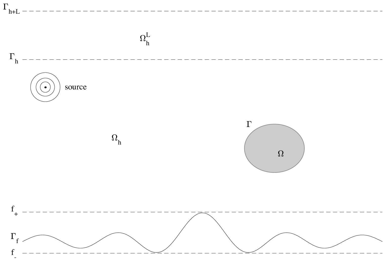
We first introduce some basic notions to be used in this paper. Throughout, let $x=(\widetilde{x}^{T},x_{3})^{T}$, where $\widetilde{x}=(x_{1},x_{2})^{T}\in{\mathbb{R}}^{2}$. Denote by $\Omega$ the bounded homogeneous, isotropic elastic body with a Lipschitz boundary $\Gamma:=\partial\Omega$ immersed in the unbounded domain $\Omega_{f}^{+}$, where $\Omega_{f}^{+}:=\{x\in{\mathbb{R}}^{3}:x_{3}>f(\widetilde{x})\}$ with the boundary $\Gamma_{f}:=\partial\Omega_{f}^{+}=\{x\in{\mathbb{R}}^{3}:x_{3}=f(\widetilde{x})\}$ described by the smooth function $f\in C^{2}({\mathbb{R}}^{2})$. We assume that $\Gamma_{f}$ lies between the planes $x_{3}=f_{-}$ and $x_{3}=f_{+}$, where $f_{-}:=\inf_{\widetilde{x}\in{\mathbb{R}}^{2}}f(\widetilde{x})$ and $f_{+}:=\sup_{\widetilde{x}\in{\mathbb{R}}^{2}}f(\widetilde{x})$ are two constants. Suppose the elastic body $\Omega$ is described by a constant mass density $\rho_{e}>0$. Let $\Omega^{c}=\Omega_{f}^{+}\setminus\overline{\Omega}$ be connected and occupied by a compressible fluid with constant density $\rho_{0}>0$. Define $\Gamma_{h}:=\{\bm{x}\in{\mathbb{R}}^{3}:x_{3}=h\}$, where the positive constant $h$ is assumed to be large enough such that $\Gamma_{h}$ is over $\Omega$, and let $\Omega_{h}=\{x\in{\mathbb{R}}^{3}:f<x_{3}<h\}\cap\Omega^{c}$. See Figure 1 for the geometric setting of the problem. Finally, define ${\mathbb{C}}_{+}:=\{s=s_{1}+is_{2}\in{\mathbb{C}}:s_{1},s_{2}\in{\mathbb{R}}\;{\rm with\;}s_{1}>0\}$.

Elastic domain. In the elastic body $\Omega$, the elastic displacement $\bm{u}=(u_{1},u_{2},u_{3})^{T}$ is governed by the linear elastodynamic equation:

where $\Delta^{*}$ is the Lamé operator defined as

Here, $\bm{\sigma}(\bm{u})$ and $\bm{\varepsilon}(\bm{u})$ are called the stress and strain tensors, respectively, given by

where $\mathbb{I}$ is the identity matrix and ${\rm NewA}\bm{u}$ denotes the displacement gradient tensor:

Further, Lamé constants $\lambda$ and $\mu$ are assumed to satisfy the condition that $\mu\geq 0$ and $3\lambda+2\mu\geq 0$.

Fluid domain. In the unbounded fluid domain $\Omega^{c}$, the pressure $p$ and the velocity $\bm{v}$ are governed by the conservation and dynamic equations in the time-domain:

Eliminating the velocity $\bm{v}$ from (2.2), we get the wave equation for the pressure $p$:

where $c$ is the sound speed and $g$ is the acoustic source which is assumed to be supported in $\Omega_{h}$ and $g|_{t=0}=0$. We assume that $p$ satisfies the Dirichlet boundary condition on $\Gamma_{f}$:

In addition, we impose the Upward Angular Spectrum Representation (UASR) condition on $p$ proposed in [6]:

for $x\in\Omega_{h}^{+}:=\{x\in{\mathbb{R}}^{3}:x_{3}>h\}$, where $\mathscr{L}^{-1}$ is the inverse Laplace transform, $\hat{\check{p}}(\xi,h)=\mathscr{F}\check{p}|_{\Gamma_{h}}$ denotes the Fourier transform of $\check{p}=\mathscr{L}(p)$ (the Laplace transform of $p$ with respect to $t$) restricted on $\Gamma_{h}$ (the definition and relationship of the Fourier and Laplace transforms are given in Appendix A), $\beta(\xi)=\sqrt{s^{2}/c^{2}+|\xi|^{2}}$ with ${\rm Re}[\beta(\xi)]>0$ and $s\in{\mathbb{C}}_{+}$.

Further, we have the following transmission conditions on the interface between the elastic and fluid media (see [26]):

(i) The kinematic interface condition

(ii) The dynamic interface condition

where $\bm{n}$ is the unit normal on $\Gamma$ directed into the exterior of the domain $\Omega$.

To be more precise, the acoustic-elastic interaction problem we consider is that a time-dependent acoustic wave propagates in a fluid domain above a rough surface in which a bounded elastic body is immersed. The problem is to determine the scattered pressure in the fluid domain and the displacement field in the elastic domain at any time. The time-dependent scattering problem can be now modelled by combining (2.1) for the elastic displacement field $\bm{u}$ and (2.3) for the pressure field $p$ together with the transmission conditions (2.6)-(2.7), the Dirichlet boundary conditions (2.4) on $\Gamma_{f}$ as well as the homogeneous initial conditions

which can be formulated mathematically as follows:

To study the well-posedness of the scattering problem (2.9), we reformulate it into a transmission problem in the strip domain $\Omega_{h}\cup\Omega$ by using the transparent boundary condition (TBC) on the plane $\Gamma_{h}$ proposed in [21]:

Then (2.9) can be equivalently reduced to the transmission problem (TP) in $\Omega_{h}\cup\Omega$:

In the remaining part of this section, we establish the well-posedness and stability of the reduced problem (2.11) by using the Laplace transform. The proof is similar to that used in [21], and so we only present the main results without detailed proofs. To this end, we take the Laplace transform of $p(x,t)$ and $\bm{u}(x,t)$, respectively, in (2.11) with respect to $t$ and write $\check{p}(x,s)=\mathscr{L}(p)(x,s)$ $\check{\bm{u}}(x,s)=\mathscr{L}(\bm{u})(x,s)$. Then (2.11) can be reduced to the problem in $s$-domain:

where $s\in{\mathbb{C}}_{+}$ and $\mathscr{B}$ is the Dirichlet-to-Neumann (DtN) operator in $s$-domain satisfying $\mathscr{T}=\mathscr{L}^{-1}\circ\mathscr{B}\circ\mathscr{L}$.

For any function $\omega(\widetilde{x},h)$ defined on $\Gamma_{h}$, the DtN operator $\mathscr{B}$ is defined by

Then the following lemma was proved in [21] (see [21, Lemmas 2.4 and 2.5]), where, for $s\in{\mathbb{R}}$ the space $H^{s}(\Gamma_{h})$ denotes the standard Sobolev space on $\Gamma_{h}$ with its norm being defined via the Fourier transform as

To study the $s$-domain problem (2.12) we introduce the Hilbert space $H:=H_{\Gamma_{f}}^{1}(\Omega_{h})\times H^{1}(\Omega)^{3}$, where $H_{\Gamma_{f}}^{1}(\Omega_{h}):=\{u\in H^{1}(\Omega_{h}):u=0\;\text{on}\;\Gamma_{f}\}$. The norm of the product space $H$ is defined by

where $\|\cdot\|_{H^{1}(\Omega_{h})}$ denotes the usual $H^{1}$-norm and $\|\cdot\|_{H^{1}(\Omega)^{3}}$ is defined by

with the Frobenius norm

It is easy to verify that

Hereafter, the expression $a\lesssim b$ or $a\gtrsim b$ means $a\leq Cb$ or $a\geq Cb$, respectively, for a generic positive constant $C$ which does not depend on any function and important parameters in our model.

The variational formulation of (2.12) can be obtained as follows: Find a solution $(\check{p},\check{\bm{u}})\in H:=H_{\Gamma_{f}}^{1}(\Omega_{h})\times H^{1}(\Omega)^{3}$ such that

where the sesquilinear form $a(\cdot,\cdot)$ is defined as

with $A:B=tr(AB^{T})$ denoting the Frobenius inner product of the square matrices $A$ and $B$.

Letting $(q,\bm{v})=(\check{p},\check{\bm{u}})$ in (2.17) and setting $\bm{\omega}=(\check{p},\check{\bm{u}})$, applying the famous Korn’s inequality [31, Chapter 10]

we obtain that

where use has been made of Lemma 1 (ii) to get the first inequality, $C=\min\{{s_{1}C_{1}}/{|s|^{2}},\rho_{0}s_{1}C_{2}\}$, $C_{1}=\min\{1,{|s|^{2}}/{c^{2}}\}$ and $C_{2}=C_{\Omega}\min\{2\mu,\rho_{e}\min\{1,|s|^{2}\}\}$. This means that the sesquilinear form $a(\cdot,\cdot)$ is uniformly coercive in $H$. By Lemma 1 (i), the trace theorem (see [21, Lemma 2.2]) and the Lax-Milgram theorem, we can obtain the following result on the well-posedness of the $s$-domain problem (2.12) or equivalently its variational formulation (2.17).

To prove the well-posedness of the reduced problem (2.11), and establish the convergence of the PML method, we need the following assumptions on the inhomogeneous term $g$:

Further, we always assume that $g$ can be extended to $\infty$ with respect to $t$ such that

By using Lemma 2 and a similar argument as in the proof of Theorem 3.2 in [21], the well-posedness and stability of the reduced problem (2.11) can be obtained.

In this section, we shall derive the time-domain PML formulation for the acoustic-elastic interaction problem (2.9). The well-posedness and stability of the PML problem can be established based on a similar method as used in the proof of Theorem 3.2 in [21]. Finally, we prove the exponential convergence of the time-domain PML method via constructing a special PML layer in the $x_{3}$-direction, based on the real coordinate stretching technique.

References

• [1] G. Bao, Y. Gao and P. Li, Time-domain analysis of an acoustic-elastic interaction problem, Arch. Rational Mech. Anal. 229 (2018), 835-884.
• [2] G. Bao and H. Wu, Convergence analysis of the perfectly matched layer problems for time-harmonic Maxwell’s equations, SIAM J. Numer. Anal. 43 (2005), 2121-2143.
• [3] J.P. Bérenger, A perfectly matched layer for the absorption of electromagnetic waves, J. Comput. Phys. 114 (1994), 185-200.
• [4] J.H. Bramble and J.E. Pasciak, Analysis of a finite PML approximation for the three dimensional time-harmonic Maxwell and acoustic scattering problems, Math. Comp. 76 (2007), 597-614.
• [5] S.N. Chandler-Wilde, E. Heinemeyer and R. Potthast, A well-posed integral equation formulation for three-dimensional rough surface scattering, Proc. Roy. Soc. London A462 (2006), 3683-3705.
• [6] S.N. Chandler-Wilde and P. Monk, Existence, uniqueness, and variational methods for scattering by unbounded rough surfaces, SIAM J. Math. Anal. 37 (2005), 598-618.
• [7] S.N. Chandler-Wilde and P. Monk, The PML for rough surface scattering, Appl. Numer. Math. 59 (2009), 2131-2154.
• [8] S.N. Chandler-Wilde, C.R. Ross and B. Zhang, Scattering by infinite one-dimensional rough surfaces, Proc. Roy. Soc. London A455 (1999), 3767-3787.
• [9] S.N. Chandler-Widle and B. Zhang, A uniqueness result for scattering by infinite rough surfaces, SIAM J. Appl. Math. 58 (1998), 1774-1790.
• [10] Q. Chen and P. Monk, Discretization of the time domain CFIE for acoustic scattering problems using convolution quadrature, SIAM J. Math. Anal. 46 (2014), 3107-3130.
• [11] Z. Chen, Convergence of the time-domain perfectly matched layer method for acoustic scattering problems, Int. J. Numer. Anal. Model 6 (2009), 124-146.
• [12] Z. Chen and J.C. Nédélec, On Maxwell equations with the transparent boundary condition, J. Comput. Math. 26 (2008), 284-296.
• [13] Z. Chen and H. Wu, An adaptive finite element method with perfectly matched absorbing layers for the wave scattering by periodic structures, SIAM J. Numer. Anal. 41 (2003), 799-826.
• [14] Z. Chen and X. Wu, An adaptive uniaxial perfectly matched layer method for time-harmonic scattering problems, Numer. Math. Theor. Meth. Appl. 1 (2005), 113-137.
• [15] Z. Chen and X. Wu, Long-time stability and convergence of the uniaxial perfectly matched layer method for time-domain acoustic scattering problems, SIAM J. Numer. Anal. 50 (2012), 2632-2655.
• [16] Z. Chen and W. Zheng, Convergence of the uniaxial perfectly matched layer method for time-harmonic scattering problems in two-layered media, SIAM J. Numer. Anal. 48 (2010), 2158-2185.
• [17] A.M. Cohen, Numerical Methods for Laplace Transform Inversion, Springer, 2007.
• [18] F. Collino and P. Monk, The perfectly matched layer in curvilinear coordinates, SIAM J. Sci. Comput. 19 (1998), 2061-2090.
• [19] Y. Gao and P. Li, Analysis of time-domain scattering by periodic structures, J. Differential Equations 261 (2016), 5094-5118.
• [20] Y. Gao and P. Li, Electromagnetic scattering for time-domain Maxwell’s equations in an unbounded structure, Math. Models Methods Appl. Sci. 27 (2017), 1843-1870.
• [21] Y. Gao, P. Li and B. Zhang, Analysis of transient acoustic-elastic interaction in an unbounded structure, SIAM J. Math. Anal. 49 (2017), 3951-3972.
• [22] T. Hohage, F. Schmidt and L. Zschiedrich, Solving time-harmonic scattering problems based on the pole condition II: Convergence of the PML method, SIAM J. Math. Anal. 35 (2003), 547-560.
• [23] G.C. Hsiao, On the boundary-field equation methods for fluid-structure interactions, in: Problems and Methods in Mathematical Physics (ed. L. Jentsch and F. Tröltzsch), Vieweg+Teubner Verlag, 1994, pp. 79-88.
• [24] G.C. Hsiao, R.E. Kleinman and G.F. Roach, Weak solutions of fluid-solid interaction problems, Math. Nachr. 218 (2000), 139-163.
• [25] G.C. Hsiao, R.E. Kleinman and L.S. Schuetz, On variational formulations of boundary value problems for fluid-solid interactions, in: Elastic Wave Propagation (ed. M.F. McCarthy and M.A. Hayes), 1989, pp. 321-326.
• [26] G.C. Hsiao, F.-J. Sayas and R.J. Weinacht, Time-dependent fluid-structure interaction, Math. Methods Appl. Sci. 40 (2017), 486-500.
• [27] M. Lassas and E. Somersalo, On the existence and convergence of the solution of PML equations, Computing. 60 (1998), 229-241.
• [28] J. Li and Y. Huang, Time-Domain Finite Element Methods for Maxwell’s Equations in Metamaterials, Springer, New York, 2012.
• [29] P. Li, L. Wang and A. Wood, Analysis of transient electromagnetic scattering from a three-dimensional open cavity, SIAM J. Appl. Math. 75 (2015), 1675-1699.
• [30] C.J. Luke and P.A. Martin, Fluid-solid interaction: Acoustic scattering by a smooth elastic obstacle, SIAM J. Appl. Math. 55 (1995), 904-922.
• [31] W. Mclean, Strongly elliptic systems and boundary integral equations, Cambridge University Press, 2000.
• [32] H.J.-P. Morand and R. Ohayon, Fluid Structure Interaction, J. Wiley, Chichester, UK, 1995.
• [33] F.L. Teixeira and W.C. Chew, Advances in the theory of perfectly matched layers, in: Fast and Efficient Algorithms in Computational Electromagnetics (ed. W. C. Chew et al.), Artech House, Boston, 2001, pp. 283-346.
• [34] F. Trèves, Basic Linear Partial Differential Equations, Academic Press, New York, 1975.
• [35] E. Turkel and A. Yefet, Absorbing PML boundary layers for wave-like equations, Appl.Numer. Math. 27 (1998), 533-557.
• [36] B. Wang and L. Wang, On L2{L}^{2}-stability analysis of time-domain acoustic scattering problems with exact nonreflecting boundary conditions, J. Math. Study 1 (2014), 65-84.
• [37] L. Wang, B. Wang and X. Zhao, Fast and accurate computation of time-domain acoustic scattering problems with exact nonreflecting boundary conditions, SIAM J. Appl. Math. 72 (2012), 1869-1898.
• [38] C. Wei and J. Yang, Analysis of a time-dependent fluid-solid interaction problem above a local rough surface, Sci. China Math. 62 (2019), https://doi.org/10.1007/s11425-017-9364-3.
• [39] C. Wei, J. Yang and B. Zhang, Convergence analysis of the PML method for time-domain electromagnetic scattering problems, submitted, 2019.