0.75
Multiscale modelling of microscale heterogeneous systems: analysis supports systematic and efficient macroscale modelling and simulation
Abstract
These are lecture notes for five sessions in the AMSI Winter School on Computational Modelling of Heterogeneous Media held at QUT in July 2019 [https://ws.amsi.org.au/].
Aim: Discuss a mix of new mathematical approaches for multiscale modelling, heterogeneous material in particular, along with corresponding novel computational techniques and issues. I include discussion of a developing toolbox that empowers you to implement effective multiscale ‘equation-free’ computation
[https://github.com/uoa1184615/EquationFreeGit.git].
Pre-requisites
undergraduate ordinary and partial differential equations, state space, trajectories, stability, bifurcations, power series solutions, separation of variables, eigen-problems and Sturm–Liouville theory; basic numerical methods for time integration of ODEs and for spatial discretisation PDEs, some perturbation methodology.
Pre-reading
recommend the review article by Kevrekidis09a. Perhaps also get an idea of centre manifolds
[https://en.wikipedia.org/wiki/Center_manifold].
Activities
sprinkled are some small activities for you.
Contents
1 Introducing a powerful approach to macroscale modelling
Contents
Let’s revisit homogenisation in some simple problems in order to clarify and resolve macroscale modelling issues. Here we primarily discuss diffusion across an inhomogeneous lattice, and comment on cognate elastic vibrations. Chapter 7 of my book Roberts2014a discusses more details, insights and applications.
This section introduces a powerful new framework for understanding and creating multiscale computational algorithms:
- •
resolves how real relates to discrete lattice/cells;
- •
applies to finite microscales in a finite macroscale;
- •
finds sharp lower bounds for allowable space and time scales;
- •
derives accurate boundary conditions for pde models;
- •
and could illuminate initial conditions, uncertainty, forcing, etc.
1.1 Homogenise period-two diffusion on a lattice—the leading approximation
Suppose a microscale lattice, as in fig. 1, has a property that diffuses with the period-two coefficients, named :
| (1) |
Define to be an average of nearby and then many arguments derive the macroscale homogenised diffusion
| (2) |
In this pde model there is no difference between diffusions and so we could imperceptibly swap—as we do in the next subsection.
The common approach of letting the microscale spacing appears a good way to derive such a pde because “” squashes a lot of difficult issues. Unfortunately, these difficult issues are often of practical importance, such as determining boundary conditions for a pde model (section 1.5).
1.2 Resolve the microscale to regularise, rather than singularise
Let’s form a system that is homogeneous on the lattice. fig. 2 shows how to do this by forming two decoupled systems that we analyse as one whole system. Usefully, the combined system is homogeneous on the lattice: every lattice point has the same equations because diffusivity always acts in the same direction, and the diffusivity always acts in the other direction. The odes are
Non-dimensionalise on the microscale length so that in effect . Writing the odes as in terms of the spatial location of the lattice points, , the differential equations for are
| (3a) | ||||
| (3b) | ||||
We analyse these near-rigorously, discover the homogenisation, and more.
1.3 An ensemble of phase shifts underpins rigorous homogenisation,
Fourier space provides a rigorous route Chen2014. However, let’s employ a corresponding direct approach (based upon Roberts2013a, which also compares with Fourier transform). We focus on ‘slowly varying’ solutions by expanding in the notionally small :
- 1.
Neglect , constant are equilibria—plotted in margin. ††margin:
- 2.
Neglect , see leads to eigen-problem: …
- •
corresponding to , and
- •
corresponding to .
So linearly, the subspace of equilibria is attractive with rapid transients —2nd plot in margin. ††margin:
- •
- 3.
Centre Manifold Theory asserts that under perturbation, such as here by small non-zero spatial gradients, the rapidly-attractive subspace is bent to a nearby rapidly-attractive manifold 11 1 A manifold is a smooth curve, surface, …, that we may parametrise with one, two, … real parameters. Read https://en.wikipedia.org/wiki/Center_manifold for a flavour of the theory. on which there is slow evolution (Carr81; Haragus2011, e.g.,)—3rd marginal plot. ††margin:
- 4.
To construct the slow centre manifold, first choose to parametrise it by the average so that . Second, some algebraic machinations (
homoDiff.txt, section A.1) constructs the slow centre manifold to be(4a) on which the parameter evolves according to the pde (4b) I invite you to substitute to verify.
For the specific case of diffusivities and substitute (4) into the microscale odes (3) and verify the odes are satisfied to residuals .
Question:
what does the time varying and its spatial derivatives mean when the underlying lattice is discrete in space? After all, such a function does not contain any information about the phase of the underlying lattice: the model pde would be the precisely same if we shifted the lattice by any fraction of the lattice spacing. So the answer is that fig. 2 does not go far enough in its doubling-up of the dynamical system. I contend the modelling only really makes sense when we regard it as modelling an infinite ensemble of lattices, each lattice at a different phase shift in the lattice spacing. Provided the ensemble is started in time in some consistent ensemble of initial conditions, then the field will evolve smoothly and model the evolution of the whole ensemble.
Microscale information resolved
The expression (4a) informs us of the microscale structure. Knowing this, and its higher-order refinements, empowers systematic modelling (cf. Daniel Peterseim’s lectures (DP), §2.4).
1.4 and underpins construction of higher order corrections
Computer algebra routinely computes higher order models, even for complicated multiphysics scenarios.
Here homoDiff.txt constructs, in terms of the mean and difference ,
But we do not have to stop there. For the example case of and , I computed to 40th order, then estimated Mercer90 that the power series for solutions converges for wavenumbers , equivalent to length scales .
- •
That is, this homogenisation should be good for predicting structures down to just two to three lattice spacings!
- •
Also, the modelling neglects transients ; that is, the model resolves time scales significantly longer than , say .
I expect similar quantitative bounds for general diffusivities (most other approaches only engender qualitative bounds).
1.5 Boundary conditions
A challenge is to derive correct boundary conditions for macroscale pde models such as the diffusion (4b). A bigger challenge is what boundary conditions should be applied to higher-order versions. Here we only answer the first, not the second: the general approach for both was developed some decades ago Roberts92c, and only relatively recently applied to this sort of homogenisation Chen2014. For definiteness I analyse the case when diffusivities are and , and leave the class of general period-two diffusivities to you.
fig. 3 illustrates the scenario near a boundary. Suppose that the microscale boundary condition on the left, , is that is specified. Then the microscale solution on the lattice must have a zig-zag structure, as shown, that reflects the alternating diffusivities, here starting on the left with the higher diffusivity . Now we expect the macroscale mean field to travel smoothly through the ‘centre’ of these zig-zags as illustrated. Consequently (fig. 3), its boundary value is generally different to the prescribed microscale value . We proceed to argue that the correct boundary condition for the diffusion pde (4b) ( and ) is the Robin condition
| (5) |
dimensionally . These express that in the scenario of fig. 3 must be a bit less than .
The key is to consider the spatial evolution away from the boundary into the interior Roberts92c; Chen2014. Specifically, because the microscale has period-two, we consider the ‘dynamics’ of the map from one pair of consecutive lattice points to the next pair: the map shown in fig. 4. Many will recognise this as the map from one ‘cell’ of the problem to the next ‘cell’.
In the slow manifold model the evolution is slow, hence time derivatives are small. Consequently, to a useful approximation we neglect time variations in the development of boundary conditions. Such time variations could be incorporated, but they obfuscate the main issues, have only a small effect, so are neglected.
To find the map from one cell to the next, without loss of generality we just derive the map from to as all the others are the same. For the specific diffusivities and , and neglecting time derivatives, the original governing odes (1) are
- •
Rearrange the first to give as a function of : .
- •
Rearrange the second to give via a function of : .
- •
Combining these two gives the map
The same relation hold for all cells/pairs, hence determines the spatial evolution away from the boundary into the interior (here an overall linear dependence upon ).
Here we derive the boundary condition just from the first two cells/pairs. Now, the macroscale field at is the average of and , that is, . Correspondingly, the macroscale field at is the average of and , that is, . But we have expressions for in terms of and , giving . Also, near the boundary the macroscale solution is very nearly linear, so to a good approximation the macroscale where the right-hand side is evaluated at , and similarly . Consequently we form the two linear equations (the left-hand sides are evaluated at )
Eliminate the unknown microscale by subtracting the second from nine times the first to give that
and hence establish the claimed boundary condition (5).
The corresponding argument, but backwards in space, provides correct boundary conditions on a right-end boundary.
What is the boundary condition for general (keep )?
Comments
- •
Curvature in the macroscale solution here only arises from an evolving out-of-equilibrium solution, so neglecting curvature in is a consistent equivalent approximation as neglecting time derivatives.
Figure 5: in diffusion through two coupled heterogenous strands, the microscale (crosses) exhibits boundary layers at each end (from Chen2014, Fig. 3). Classic arguments give bcs for macroscale pdes that incorrectly predict the red line. Our approach caters for the microscale boundary layers and heterogeneity to give bcs that correctly predict the blue line. - •
In more complicated problems there are boundary layers at each boundary, shown for example by fig. 5, that we cater for in a more general argument Roberts92c; Chen2014.
1.6 Microscale heterogeneous mechanical media
What if the system illustrated by fig. 1 is that of a mechanical system. For simplicity, say there are unit masses at every microscale lattice point, connected by springs to its two neighbours. The heterogeneity is that the springs are of alternating strengths and . We derive that the appropriate macroscale homogenisation is the classic wave pde—with higher-order modification.
Let denote the displacement of each mass, and denote the velocity of each mass. Then the microscale odes are modified from (1) by changing “” to “ and ”. As in sections 1.2 and 1.3, non-dimensionalise and embed in an ensemble of phase shifts.
- 1.
As before, focus on the slowly-varying solutions by regarding as ‘small’.
- 2.
The eigenvalue equation become and indicating two slow modes among fast oscillations of frequency . Thus linearly, the slow subspace is which acts as the centre of oscillations, instead of being exponentially quickly attractive.
- 3.
Theory asserts that under perturbation there exists an ‘asymptotically close’ system that has a slow manifold, free of the fast oscillations, and tangent to the slow subspace (Roberts2018a, §2.5, this is a backward theorem!).
- 4.
Almost the same algebraic machinations (
homoVibr.txt, section A.2) constructs the slow manifold to be(6a) (6b) on which the parameters evolves according to the pde (6c) I invite you to substitute to verify.
The macroscale pde (6c) is the classic wave pde for the mechanical medium. Straightforward higher-order analysis constructs higher-order models that show the waves are at least a little dispersive.
Boundary conditions for the wave pde may be derived as in section 1.5.
Fast waves may resonate
However, in nonlinear wave systems, one important difference is that the slow macroscale evolution is different when there are fast waves present, compared to when the fast waves are absent (Roberts2014a, Ch. 13): the difference is typically quadratic in the fast wave amplitude (e.g., Stokes drift in water waves). For example, consider the toy nonlinear system
Fast waves of frequency are in , so the slow manifold is exactly. On this always decays to zero. But in the presence of fast waves the long-term solution is fundamentally different: put in polar coordinates and then , and . So solutions with fast waves have of the slow manifold prediction. This mean effect of fast waves is independent of the frequency!
See a similar effect in , and via the coordinate transform that , and . What is the overall -evolution?
1.7 Optional: Nonlinear pattern formation is analogously rigorously supported
Recall that section 1 discussed that modelling an ensemble of phase shifted diffusivity was a rational way to form macroscale models of heterogeneous material. A similar approach works when the heterogeneity is an emergent phenomena of the system.
Pattern formation is a common phenomena in science and engineering: for examples, the stripes on a zebra, the spots on a leopard, and the ordered arrays of clouds. Let’s overview briefly one of the basic toy problems in this class. Consider the small amplitude solutions of the Swift–Hohenberg system in one space dimension: a field satisfies the nondimensional nonlinear ‘microscale’ pde
| (7) |
on a domain of large extent in . For parameter small, the slow marginal modes are . The aim is to derive, as a macroscale model over large , the well-known Ginzburg–Landau pde
| (8) |
governing the complex amplitude of oscillatory patterns (Cross93, e.g.).
The trick to a rigorous approach is to embed the pde (7) in the larger problem of analysing the ensemble of all phase shifts of the pattern (Roberts2013a, §2.5, §3.3). As indicated schematically in fig. 6, and in terms of a new ensemble/phase variable , consider a new field satisfying the pde
| (9) |
for , where the field is -periodic in . Given any solution of the pde (9), elementary calculus shows that, for any chosen fixed phase and using that is -periodic in , the field (along the blue lines in fig. 6) is a solution of the Swift–Hohenberg pde (7). Thus modelling of the dynamics of the ensemble pde (9) immediately leads to models for the dynamics of the Swift–Hohenberg pde (7).
This ‘embedding’ approach immediately makes new sense of the multiple space scales that others introduce, such as Elliot Carr’s and . The ‘cell problem’ here becomes solving in for the structure, given slow variations in , but now with a well defined geometry.
The macroscale modelling of the ensemble pde (9) may be done via rigorous local Taylor expansions about an arbitrary station (fig. 6). Such local models are typically only weakly coupled to neighbouring locales, and so the collection of local models generates a global pde as the macroscale model Roberts2013a. Here we would derive the Ginzburg–Landau pde (8).
The rigorous ensemble embedding here replaces heuristic multiple space and time scale assumptions traditionally employed in the asymptotic analysis of patterns (Cross93; Vandyke87, e.g.).
1.8 Open problems
- •
Provide tools to automatically construct such models and boundary conditions for users, tools analogous to the web services I operate (Roberts07d, e.g.).
- •
Deduce quantitative bounds on the spatio-temporal resolution of many of the classic macroscale pde closures in multiscale systems (mainly only for linear problems).
- •
What are appropriate initial conditions (Roberts89b, e.g.) for a macroscale pde given that the microscale is spatially discrete, and we only derive the macroscale by an embedding ensemble?
- •
Develop Backwards Theory for centre/stable/unstable/slow/fast manifolds: that is, instead of “for a given system provided restrictions there exists …” establish “generally there exists a nearby system for which exact manifolds are …” (Grcar2011, aka) Roberts2018a.
- •
Rigorously support and practical procedures to develop boundary conditions for macroscale pdes in 2D or 3D spatial domains.
- •
What if the microscale is stochastic? (Roberts06k, may inspire an approach)
2 Multiscale computation of microscale systems
Contents
Suppose that in some problem
- •
we have a trustworthy microscale simulator,
- •
and a ‘spatial’ domain so large the microscale code is not feasible,
- •
but we do not know and/or cannot derive a macroscale closure.
Answer: use the microscale simulator on small patches of space (fig. 7), with the patches coupled over unsimulated space, craftily, so that we make macroscale predictions. Such predictions are computed relatively quickly when the patches are a small fraction of the whole domain. sections 2.5 and 2.6 show that the macroscale homogenisation of the coupled patches is accurate in cases when we do know the macroscale closure.
2.1 One Patch to rule them all, …
The simplest scenario is just one patch coupled to distant boundary values. fig. 8 shows one small patch of length in a domain . Inside the patch the microscale is that of heterogeneous, period-two, diffusion. This microscale patch is to be coupled to the boundary values at the distant of . How can we couple to make correct predictions?
Here we know the desired predictions. The macroscale closure is that (approximately) for effective homogenised diffusivity . So that, for example, if the macroscale field is approximately parabolic, , then … the macroscale closure gives . We compare the patch scheme with this ode.
Within the microscale patch, the microscale equations, from (1), in the interior of the patch are
| (10a) | ||||
| (10b) | ||||
| (10c) | ||||
| where the -factor on the left-hand side caters for the microscale lattice spacing of . Whereas section 1 non-dimensionalises the lattice spacing to , here we scale the macroscale domain length to two and so the microscale length scale is denoted . | ||||
But we need two edge values for the patch, at . These come from macroscale coupling with the boundaries—although in general from coupling with neighbouring patches. Let’s pose the predicted macroscale is classic parabolic interpolation through the two given boundary values, namely zero at , and the evolving centre-patch value of at the centre-patch . That is, the predicted macroscale is . Then the two patch-edge values are taken to be this field evaluated at the edges , namely the microscale
| (10d) |
This coupling completes the patch simulation equations.
What are the dynamics of the patch scheme? It is linear so find a general solution, after substituting (10d), via seeking . That is, find the eigen-values and eigen-vectors of matrix
In terms of , this matrix’s characteristic polynomial factors to
That is, and . In the interesting cases of small patches, small , these give the three eigenvalues
For small the last two are large negative eigenvalues and the first is relatively small. Thus, quickly, after a cross-patch diffusion time of , all patch solutions lie on the subspace corresponding to the small eigenvalue. On this slow subspace they evolve nearly as . This rate, , exactly matches the macroscale closure pde. The patch scheme gives good macroscale predictions despite solving the microscale on only the small fraction of the domain.
What does the patch scheme predict when the boundary condition at is replaced by ? For simplicity set diffusivities and . How does the prediction compare with the macroscale homogenisation?
2.2 Automatic macroscale closure
I think this amazing! We only solved the microscale equations on a patch of length and yet predict the macroscale homogenisation. Similarly for executing microscale code instead of solving. The patch size could be tiny and we still get an accurate homogenisation. We have not coded into the patch scheme any knowledge of the homogenisation, yet the scheme effectively, and on-the-fly, forms an accurate macroscale closure.
There are two caveats here. Firstly, in the scheme analysed we only predict one macroscale mode over the domain, the parabola . But what about other macroscale modes such as and ? To resolve all three of these modes we would need three patches in the domain. In general, patches resolve macroscale modes (section 2.5).
Secondly, let’s check what happens with different number of lattice points in the patch.
Computer algebra, onePatchHomo.txt (section A.3), easily checks for patches of size .
All cases have
- •
negative eigenvalues of large magnitude characteristic of rapid sub-patch diffusion, and
- •
one small negative eigenvalue giving the effective macroscale homogenised diffusivities of table 1.
Patches of size with even are macroscale correct (and odd are increasingly accurate as increases). This illustrates the general rule that it is best if the half-size of a patch is an integral multiple of the microscale periodicity (DP, and Bunder2013b, §5.2).
Consider DP’s first problem but over : with and for integer . Form one patch with edge conditions from the macroscale parabolic interpolation . Solve exactly within the small patch (aided by symmetry) to discover the solution in the patch is that of the exact whole domain solution!
2.3 Optional: Nonlinear diffusion in one patch
How does a patch of nonlinear dynamics perform? Let’s consider the nonlinear pde example for field of
| (11a) | |||
| subject to boundary conditions . | |||
Solve only on the small patch . The macroscale interpolated field is, given the centre-patch value that . So the edge values on the patch are that
| (11b) |
What are the predictions when we only solve (compute) pde (11a) on the small patch?
- 1.
Embed the problem in a family of problems parametrised by , , through generalising the edge condition (11b):
(12) We use a theory based at to access results that hold for full coupling, .
- 2.
Equilibria? constant and . Call the constant for compatibility—see marginal plot. ††margin:
- 3.
Linearise: seek for small and negligible . Then the pde and edge conditions become …
Seek solutions via separation of variables, , and find … eigenvalues and eigenfunctions are
as well as some generalised eigenfunctions for —schematic 2nd marginal plot. ††margin:
- 4.
Emergence theory? Because there is a zero eigenvalue with the rest negative and, centre manifold theory (Carr81; Haragus2011, e.g.) asserts the system (12) possesses a 2D slow centre manifold on which the system evolves, . Further, the solutions on the slow centre manifold attract all nearby ones roughly as —schematic 3rd marginal plot with red centre manifold. ††margin:
Consequently, provided evaluation at is valid, the original patch system (11) possesses a quickly attractive 1D slow centre manifold on which the system evolves . Again, on a cross-patch diffusion time all solutions of the patch system (11) approach a 1D ode which turns out to be the appropriate macroscale dynamics.
- 5.
Construction: I chose this nonlinear problem as it is straightforward to verify the exact slow centre manifold is precisely
To verify, substitute into (12) ….22 2 This example also nicely illustrates two ways centre manifold models ‘break down’. For parameter the centre manifold is attractive, but solutions within the centre manifold explode to infinity in finite time, via . Whereas for parameter the centre manifold exists and solutions within it are stable for all time, but the centre manifold surely no longer attracts all nearby solutions as the nonlinear diffusion coefficient, , is negative for .
Hence, at , the original patch system (11) for has the attractive exact slow centre manifold
(13)
The patch slow centre manifold (13) also happens to be exact for the whole domain pde (11a). But here we discover the exact dynamics, , ‘economically’ by solving the pde only on a microscale patch, and using interpolation over unsolved space to fill in the macroscale gaps.
What (little) would change in this analysis if the macroscale boundary conditions are at ? where parameter .
2.4 A basic atomic simulation
So far I have discussed several toy problems. Let’s have a brief look at the realistically complicated scenario of atomistic simulation, and a patch simulation.
Consider a long domain , with thin square cross-section , filled with a monatomic gas. We want to simulate the macroscale diffusion of heat along the long thin domain. Here we know the macroscale is the diffusion pde , although maybe not know the diffusivity , nor its temperature/pressure dependence. But let’s pretend we do not know even the form of this macroscale closure. Instead, let’s make a macroscale prediction for the diffusion of heat using a microscale atomic simulation within an single patch Alotaibi2017a.
The most straightforward atomic simulation to code is that of the motion of atoms, with interatomic forces determined from the classic Lennard-Jones potential, in a triply periodic, cubic, domain. fig. 9 shows such a simulation with atoms over a short microscale time.
Similarly, Lattice–Boltzmann simulations easiest to code when periodic (as commented by CSF).
Question: how can we use such a microsimulation code in a patch scheme? fig. 10 shows the simplest patch scheme. We position just one micro-domain, a cube of side , centred at , and filling the square cross-section of the domain. The distant boundaries of the macro-domain are at , on which we impose temperatures .
But the micro-code patch is triply periodic, so we cannot specify boundary values on the edge of the patch, because the patch has no edge! Instead we control the patch. Define four equi-sized regions in the patch as shown in fig. 10:
- •
the core region—we estimate the macroscale temperature at from the kinetic energy of the atoms in the core;
- •
two action regions in which we apply a proportional controller to heat/cool the atoms depending upon whether the macroscale interpolated temperature through is less/more than the kinetic energy of the atoms in the particular action region;
- •
and an ‘unmentioned’ region whose role is to complete the microscale periodicity.
|
temps , , |
|
|---|---|
| (a) | time |
fig. 11 shows the result. There is an initial equilibration transient which occurs on a time-scale almost too small to see on this time-axis. After that rapid transient, a relatively cool patch, temperature about , gradually heats up, with more heat flux from the right-end at , than from the left-end at . Over the macroscale time shown, the atoms in the patch heat up to the equilibrium temperature , with fluctuations due to the microscale chaos in the atomic motion. Because the macroscale equilibrium temperature should be linear from left to right, in the final atomic ‘equilibrium’ the action regions have temperatures , by roughly equal amounts.
This controlled periodic-patch scheme does appear to predict reasonably correctly the macroscale dynamics. We analysed the dynamics of such a single coupled periodic patch, and multiple coupled periodic patches, to determine optimal control parameters (Alotaibi2017a, SS4,5).
2.5 Classic interpolation couples patches consistently,
Let’s turn now to the issue of coupling the computation on many microscale patches across a large macroscale domain. The simple answer is to couple by providing edge values for the patch computation via classic Lagrangian interpolation over the macroscale gaps of the patch centre-values (Roberts06d, e.g.). We show that the homogenisation of the dynamics of patches and gaps is reasonably accurate.

fig. 12 illustrates an example applied to the field satisfying Burgers’ pde . We only compute on the patches, and not at all in the gaps. Initial rapid transients, only just visible in the initial instants, decay to smooth sub-patch fields that then interact and evolve over macroscale space-times.
Equation-Free Toolbox
33 3 https://github.com/uoa1184615/EquationFreeGit.gitExecute patchConfig1() to see fig. 12 generated by the example code near the start of the function.
In the macroscale domain place a grid, spacing , with grid points . Centre a microscale patch, of size , at each grid point so the th patch covers . Let denote the field in the th patch, but often it is convenient to use the th patch-centric space variable , for scale ratio , to describe sub-patch structures, so usually we consider . The macroscale field is then formed by interpolating over the gaps all the centre-patch values .
To create the inter-patch coupling, define the macroscale shift operator and equivalently , as appropriate for steps on the coarse grid size , and then its inverse gives and . Consequently, and which naturally holds for all real . In particular, the patch edge-values need to be the interpolated macroscale: that is, since the patch-edges are at and patch-centre is at for scale ratio ,
| (14) |
The patch scheme is then to compute/solve the microscale code/pde in each of the patches, , coupled by using (14) to specify the patch edge-values where denotes the centre value of the th patch.
But how do we compute the required edge-values ? Answer: via some classic identities for discrete operators (npl61, p.65, e.g.):
| difference | |||
| mean | |||
| shift |
Then, applied to for the edge values, and recall the scale ratio ,
| (15a) | ||||
| (15b) | ||||
| (15c) | ||||
| (15d) | ||||
| (15e) | ||||
We approximate by truncating at some line: truncating at (15a) is locally second-order parabolic interpolation; truncating at (15b) is locally fourth-order quartic interpolation; and so on.
A simple test of accuracy? Linear diffusion , with macroscale periodicity of and determine the accuracy of the macroscale modes. The precise eigenvalues should be for (except for , all are multiplicity two). table 2 gives the numerical results and shows the macroscale eigenvalues, those for , are accurately determined by the patch scheme: the errors are as befits the fourth-order interpolation across gaps. The rightmost column of table 2 gives the leading microscale eigenvalues which are several orders larger, corresponding to the decay of sub-patch modes on a sub-patch diffusion time . The patch scheme with multiple patches appears to make successful macroscale predictions, despite only computing on separated small patches of the domain.
| 1 | 2,3 | 4,5 | 6,7 | ||
|---|---|---|---|---|---|
| 4 | n/a | ||||
| 8 | |||||
| 16 | |||||
| 32 | 0 |
Similarly, consistency errors are for stencil width for general pdes.
Here we only discuss the case when the microscale simulator needs field values on the patch edges. Analogous formula successfully interpolate derivative values to the patch edges if needed by the microscale simulator Roberts04d, or Robin conditions, or two-point conditions Roberts06d.
2.6 and with dynamical systems support
This section describes one way to provide theoretical support for the patch scheme in its macroscale modelling of nonlinear microscale systems. My trick is to embed the patch scheme in a one parameter family of schemes. The introduced parameter controls the strength of the inter-patch coupling: when the patches are fully coupled; when the patches are isolated from each other. We use a theory based at to access results that hold for full coupling, .
Introduce the parameter into the inter-patch coupling (15) so it takes the modified form
| (16a) | ||||
| (16b) | ||||
| (16c) | ||||
| (16d) | ||||
| (16e) | ||||
Then, instead of (14), the patch-edge values are determined by
| (17) |
for scale ratio . Observe that terms multiplied by flag a patch communicating with its nearest neighbours, those terms multiplied by flag communication out to next-nearest neighbours, and so on. 44 4 That is, parameter empowers us to order the system’s interactions between all the patches (maybe analogous with Feynman diagrams in physics). Hence, analysing to asymptotic error means that a patch communicates with patches to each side of itself.
Incidentally, when the patches overlap and empowers algebraic novel and accurate discretisations based upon the pde telling us the sub-grid structures (section 3.4). Then , the so-called holistic discretisation.
To get the flavour of the theoretical support this patch coupling engenders for our multiscale computational of patches and gaps, let’s consider this -parametrised scheme applied to Burgers’ pde with say patches.
- 1.
Equilibria? When each patch is isolated, and so constant independently in each patch is an D subspace of equilibria (cf. DP’s finite element space ); that is, for —see schematic marginal plot. ††margin:
As it is easiest we analyse about the equilibria , but in principal we could generalise to being global in . The analysis is local in coupling parameter , but evidence indicates the locale often extends to include —the case of interest.
- 2.
Linearisation: small perturbations to the equilibrium then satisfy, upon changing to , the pde such that, from (17) with , . As coupling , each patch is isolated and the analysis here is the same over all patches. As in section 2.3, seek solutions via separation of variables, , and find eigenvalues and eigenfunctions are
as well as some generalised eigenfunctions for —2nd schematic marginal plot. ††margin:
- 3.
Emergence theory? Because there is a zero eigenvalue for each of patches, with all other eigenvalues, centre manifold theory (Carr81; Haragus2011, e.g.) asserts the pde on patches coupled by (17) possesses an D slow centre manifold on which the system evolves , for some domain of finite . Further, the solutions on this slow centre manifold attract all nearby ones roughly as . That is, on a cross-patch diffusion time all solutions of the multi-patch system approach the dynamics of a slow macroscale D system—3rd schematic marginal plot with red centre manifold. ††margin:
This slow centre manifold system turns out to be an appropriate macroscale system at full coupling .
- 4.
Construction: computer algebra handles the tedious details. It eventuates that on the slow centre manifold, the th patch has sub-patch field (cf. DP’s )
Here, this sub-patch field is the classic parabola formed from local first and second derivative estimates. Higher-order linear terms are likewise. However, microscale heterogeneity, non-linearity or odd derivatives in the pde (section 3.4) generate non-classic sub-patch structures that represent non-trivial out-of-equilibrium structures on the sub-patch microscale (Roberts00a, §3, e.g.).
The evolution on the slow centre manifold is
Choosing to truncate with coupling errors and then evaluating at full coupling gives classic spatial discretisations of the diffusion pde, with errors classically recorded as . That is, the slow centre manifold emergent dynamics of the coupled small patches is precisely a sound model of the macroscale dynamics.
The same conclusion holds when the nonlinear terms are explored, and also holds in two space dimensions Roberts2011a.
We conjecture the patch-scheme is similarly good for scenarios where we do not know the macroscale closure.
2.7 Open problems
- •
For periodic patches: investigate other controllers? their optimal control? extend supporting analysis to a useful range of macroscale pdes? including stochastic? develop coupling in multiple directions, not just 1D? develop boundary patches?
- •
A trendy activity is to get Deep Neural Networks (!) to ‘learn’ a macroscale closure from microscale simulations (section 3.4): compare such dnns with algebraic closures (BarSinai2018; Roberts00a, e.g., cf.).
- •
Roberts08l; Roberts2011a provide theoretical support for the patch scheme on a regular grid in 2D: it should be straightforward to extend to more space dimensions; and may be challenging to extend to an unstructured grid of patches.
- •
We are currently working on developing moving patches with the aim of capturing shocks by resolving them on a microscale patch and without assuming any Rankine–Hugoniot conditions.
- •
Develop the toolbox to patch functions for non-periodic macroscale boundary conditions, to higher-D, to effectively parallelise, and so on.
3 Macroscale computation of microscale spatial complexity
Contents
Recall that section 2 discussed the amazing automatic homogenisation of one patch period-two heterogeneous diffusivity. Here we discuss multiple patches and the corresponding automatic macroscale homogenisation of the patch scheme.
We are developing a suite of Matlab/Octave functions to empower users to take advantage of the patch scheme and other multiscale techniques. Download the current version from GitHub. 55 5 https://github.com/uoa1184615/EquationFreeGit.git
Many of the main functions, if invoked with no arguments, will execute a basic example.
For example, executing configPatches1() draws fig. 12 arising by simulating Burgers’ pde within eight patches.
The user manual, eqnFreeUserMan-newest.pdf, is in the main folder and should suffice for most users.
66
6
Doc/eqnFreeDevMan.pdf documents full details of the toolbox functions.
3.1 Couple patches of microscale heterogeneous diffusion for macroscale accuracy
The script homogenisationExample simulates the basic homogenisation introduced by section 1, but now on multiple patches, albeit still in 1D.
Recall the remarkable result that if configured so that the patch half-width is an integral multiple of the microscale period, then the patch scheme simulates the exact macroscale homogenisation (Bunder2013b, §5.2).
The overall plan of the code is similar to that discussed in section 5.1, but microscale details are different. The user has to drive two functions in the toolbox:
- •
configPatches1()configures the arrangement of patches and sub-patch microscale lattice in the domain; - •
patchSmooth1()computes the patch edge-values so that a user’s function computes a time-step/derivative of the sub-patch structure.
The overall plan is the following:
- 1.
invoke
configPatches1()and other initialisation - 2.
user time loop/integration, e.g.
ode15s- (a)
invoke
patchSmooth1()- i.
patchEdgeInt1()computes patch edge values - ii.
user function
heteroDiff()gives time derivatives
- i.
- (a)
- 3.
process results
The code initialises the heterogeneous diffusion coefficients and periodicity
1 mPeriod = 3 2 cDiff = exp(randn(mPeriod,1))Then it invokes configPatches1() to configure a -periodic domain with nine patches coupled with fourth-order interpolation. Each patch is chosen to be of size ratio and to contain precisely two periods of the microscale heterogeneity.
1 global patches 2 nPatch = 9 3 ratio = 0.2 4 nSubP = 2*mPeriod+1 5 Len = 2*pi; 6 ordCC = 4; 7 configPatches1(@heteroDiff,[0 Len],nan ... 8 ,nPatch,ordCC,ratio,nSubP);The code takes advantage of the patch struct patches to communicate the specific heterogeneous coefficients, identical for each patch (could they be different?),
1 patches.c = repmat(cDiff ... 2 ,(nSubP-1)/mPeriod,1);to the user’s microscale function heteroDiff().
1 function ut = heteroDiff(t,u,x) 2 global patches 3 dx = diff(x(2:3)); % space step 4 i = 2:size(u,1)-1; % interior patch 5 ut = nan(size(u)); % preallocate 6 ut(i,:)=diff(patches.c.*diff(u))/dx^2; 7 end
The example script then integrates in time from some initial condition using ode15s()
1 u0 = sin(patches.x) ... 2 +0.4*randn(nSubP,nPatch); 3 [ts,ucts] = ode15s(@patchSmooth1 ... 4 , [0 2/cHomo], u0(:));To visualise the results, plot as before
1 xs = patches.x; xs([1 end],:) = nan; 2 mesh(ts,xs(:),ucts’), view(60,40) 3 xlabel(’time t’), ylabel(’space x’) 4 zlabel(’u(x,t)’)
Accuracy?
Bunder2013b [§5.2] analyse the scenario and assure us that the macroscale predictions are correct.
We may verify here by computing the Jacobian of the patch scheme, and then the small magnitude eigenvalues correspond to the macroscale modes.
I wrote the script homogenisationAccuracy to do this.
It normalises the heterogeneous diffusions so their harmonic average is one and so the homogenised pde is .
Then on the domain the macroscale eigenvalues should be for integer .
The script uses spectral interpolation to ‘eliminate’ interpolation errors.
Executing the script gives answers such as the following.
mPeriod =
     3
cDiff =
        5.887
        21.52
      0.35924
nPatch =
     9
ratio =
          0.1
nSubP =
     7
lamFast =
      -5440.7
lam0 =
      -7.7342e-12
      -0.9997
      -0.9997
      -3.9947
      -3.9947
      -8.9731
      -8.9731
      -15.915
      -15.915
These macroscale eigenvalues are close to . The differences are not errors, the differences are due to the small but finite size of the microscale discrete lattice causing higher-order terms in the effective macroscale pde: it should be . Reduce the ratio to lessen higher-order effects from the microscale.
Projective integration
There is a large spectral gap between these macroscale modes and the leading eigenvalue of the sub-patch modes, by a factor of roughly a thousand.
These multiscale schemes are typically extremely stiff so prefer projective integration (section 4).
The script homogenisationExample proceeds to additionally use projective integration in time, and fig. 13 illustrates that the resulting simulation only computes on patches in space-time.
3.2 Avoid buffers in general homogenisation
So far we have addressed the scenario where we know the periodicity of the microscale heterogeneity. What if we do not? or if the microscale is random? These were explored by Bunder2013b [§5.3].
fig. 14 illustrates a more general patch of size lattice points. Instead of defining the patch macroscale value as the centre patch value, we define it to be the average over a core region of width at the centre of a patch. Since the macroscale is an average, the coupling conditions also need to be phrased in terms of corresponding averages. Hence patches are coupled by defining action regions of width at the edges of each patch, and then requiring that the average over an action region be the interpolated macroscale averages. This forms a more general patch scheme.
We explored this more general patch scheme in simulating the macroscale dynamics of microscale heterogeneous diffusion for cases where we do not ‘know’ the microscale periodicity. fig. 15 shows we varied the size of the core/action regions, assessed the error in the macroscale predictions over a range of microscale periodicities. Be particularly interested in the commonly espoused plausible idea that there should be a sizeable buffer (grey) between the action regions and the core region to allow the sub-patch solution to ‘heal’.
fig. 16 shows the log-error as a function of the core size relative to the patch size. A remarkable feature of fig. 16 that the error is minimised for core . That is, for minimum error in macroscale predictions make the core and action regions overlap slightly! Making the core and action regions abut without overlapping is also reasonable if you prefer as . It appears that we never need buffers.
3.3 How do communication delays affect such simulations?
Recall we envisage that in large problems the spatial patches will be distributed across many processors in parallel. In that scenario much of the microscale computation may be done efficiently on each processor. However, then the inter-patch coupling incurs real-time expensive inter-processor communication. In the scheme described so far, such inter-patch/processor communication occurs every microscale time step. Such communication would slow the computation severely.
Alternatively, maybe we could communicate the inter-patch coupling less often? Bunder2015a explored the effect on accuracy of communicating coupling on an intermediate time meso-scale—longer than micro-times, and shorter than macro-times. fig. 17 illustrates the idea.
For simple diffusion on a lattice , we could obtain complicated analytic formulas across many scenarios. To help fill-in the communication ‘gap’ from time to time we considered communicating not only the neighbouring macroscale values, but also their first time derivatives. During a time coupling errors penetrate into the core of each patch from the edge regions. The aim is to keep small the errors in the patch-core.
fig. 18 shows that by using larger patches, here half-size lattice points, we protect the patch-core from the lack of updates to the patch edge-values. Here the error in the core is at the round-off level. Increasing the number of time derivatives communicated decreases the error. fig. 18 shows the results for all cases where a core-average over points in the patch is the macroscale quantity communicated.
fig. 19 shows the effect of varying the meso-scale time of communication, . As expected the errors increase with , and decrease with increasing patch width. Similar behaviour was seen in 2D spatial patch simulations.
Limiting inter-patch/processor communication to meso-times may speed up large-scale simulations by factors of – (Bunder2015a, §6.2). But in limited communication we need some ‘buffers’.
3.4 Algebra ‘learns’ good macroscale discretisations
For efficient computation within, we want small patches. But when algebra resolves the sub-patch structure then the patches can be any size. Patches that overlap, , appear most appealing—the so-called holistic discretisation Roberts00a.
This approach provides a framework for systematically constructing sub-grid structures determined by the problem—like DP, but non-‘variational’—in contrast to fd/fe/fv imposition.
We explore the macroscale dynamics predicted by overlapping patches. We find formulas for sub-patch structures and macroscale evolution that are cognate to trendy efforts that analogously try to ‘discover’ macroscale closures by invoking Deep Neural Networks on extensive numerical simulations (BarSinai2018, e.g.).
Here let’s explore governed by the linear advection-diffusion pde
| (18) |
Define a macroscale grid of equi-spacing . Let the th patch be so it stretches from to , and the field on the th patch be for sub-patch variable .
2D space? There are several ways to generalise to 2D Roberts08l; Roberts2011a. The overlap means a patch shares half of itself with each of four nearest neighbours. Hence the overlap empowers ‘channels’ to be continued or otherwise correctly from one patch to the next—in principle (as required by BL in so-called ‘skins’).
In 1D the coupling between patches is particularly simple as the edge of each patch is the neighbouring centre-patch. Then the embedded classic interpolation (17) becomes simply
| (19) |
in terms of coupling parameter , and local space variable .
As in patches, the parameter controls the locality in space of a hierarchy of approximations: working to ‘errors’ means a stencil width of .
Our quest is to find that the macroscale dynamics of the patch system () is good.
- 1.
Equilibria? When the coupling , the patches are isolated, and equilibria are that constant independently in each patch. Defining the amplitude to be the centre-patch value, , these constants are . ††margin: The schematic marginal plots of section 2.6 apply here also.
- 2.
Linearise: each patch is the same with linearised problem such that . Each patch has a zero eigenvalue, and an infinite number of negative eigenvalues: maybe .
- 3.
Hence, solutions exponentially quickly approach a slow centre manifold/subspace that is parametrised by and (Carr81; Haragus2011, e.g.,).
- 4.
Construct? 77 7 Although the problem is linear, the construction of a model is nonlinear through the chain rule that and we must determine both and . Seek sub-patch fields such that . Substitute into coupled pde () and the -terms require
Although tedious, the solution is straightforward (Roberts00a, §3):
(20a) (20b) (20c) Higher orders in coupling are best left for computer algebra.
- 5.
Interpret? Set coupling parameter to predict at full coupling.
- •
Expression (20a), added to , gives the sub-patch structures ‘learnt’ by the algebra from the pde. These structures are not imposed by us on the physical problem (cf. classic finite element/volume/differences). These out-of-equilibrium structures ‘know’ relevant sub-patch dynamics from the pde.
- •
Higher order analysis in coupling , say to errors , would learn more about the sub-patch structures by accounting for the influence of patches up to -distant (Roberts00a, §3).
Figure 20: the enhanced macroscale dissipation (20c). - •
The macroscale dynamics are the odes from (20b) and give us as good an approximation as one could expect from any three-point stencil. Importantly, the effective dissipation (fig. 20) is enhanced so that as advection increases then morphs seamlessly into an upwind discretisation. The odes are stable for all —there is no cfl constraint.
- •
The algebraic closure ‘learnt’ here is valid globally in , and : the closure is not limited by the finite extent of the simulations typically underlying any machine learning.
- •
Modelling in general? Dynamic macroscale models are nonlinear transformations of the microscale system, here (fig. 20), and ‘harmonic mean’ in homogenisation. So endemic linear arguments necessarily have deficiencies in dynamics. Consequently, “the whole is more than the sum of the parts” because the whole is a nonlinear transform of the parts.
3.5 Open problems
- •
Ongoing research is exploring patch configurations that automatically homogenise 2D heterogeneous diffusion to high accuracy.
- •
Further explore ‘symmetry’ preserving patch/holistic coupling conditions Roberts08l especially for general heterogeneity as discussed by DP (Bunder2013c, cf.), or piecewise linear based coupling that also connects to splines Jarrad2016a.
- •
Convincing people that negative probabilities and negative concentrations are ok (e.g., Roberts2014a, Exercise 5.2).
- •
Develop the toolbox to patch functions coping with stochastic sub-patch structures.
- •
Explore meso-time communication in practice, and for advection for which I expect a worse performance.
- •
Incorporate tolerance to hardware failure as in massive parallelism, needed for the largest problems, it is likely that one of the millions of cpus will fail during a computation.
4 Projective integration computes only on small bursts of time
Contents
Historically, projective integration was the first ‘equation-free’ technique (Gear02; Gear02b, e.g.). As shown in the example of fig. 21, the aim is to use small bursts of microscale simulation (solid lines) to then extrapolate forward in time, over unsimulated time (dotted), to predict the next macroscale value (circles), and then repeat.
Importantly, in this scheme we do not impose our subjective opinion of what should be ‘frozen’ macroscale variables. Some other multiscale methods do subjectively ‘freeze’. Instead projective integration always deals with the full dynamics of the system’s complete out-of-equilibrium interactive exchange of information to and fro between micro- and macro-scales.
4.1 Accuracy and stability for such schemes,
Let’s see what happens in the simplest projective integration, akin to Euler method Gear02b. You execute a burst of some code and it takes very many microscale steps in time from , say, to arrive at some end-burst time . For simplicity, and unknown to you, let’s suppose the system is simulating . At the end of the burst, , you get the two results that and it is changing in time as . Extrapolating over time-gap then predicts, without any further expensive microscale simulation, that
Repeat times to predict for growth factor, where ,
| (21) |
- •
fig. 22(left) compares the growth factor with the exact and shows that for accuracy we need small ; that is, the macro-time-step must be smallish compared to the time-scale of macroscale interest.
- •
fig. 22(right) shows that for stability the burst needs to be long enough so that (more precisely)—although the bound is much better for a multi-scale system.
But in general we must consider large-scale systems, not just one variable.
Systems are locally linear
Consider a general system of odes . Such nonlinear systems are locally linear by Taylor’s theorem. Suppose is a solution, then nearby solutions satisfy
| (22) |
We see this by substituting into the system : the left-hand side is whereas by Taylor about the right-hand side
Cancelling and dividing gives the linear system (22).
Recall that, generically, the linear system is fully understood by diagonalisation. Generally there exists a linear coordinate change , the columns of are eigenvectors, such that for diagonal matrix of eigenvalues . By superposition we thus primarily need to consider over all the spectrum of eigenvalues of the Jacobian .88 8 Neglecting issues associated with a time varying Jacobian; for example, see the Marcus–Yamabe system.
Fast-slow multiscale systems
Now in a multiscale system, including those with microscale heterogeneity, the spectrum divides into two ‘clusters’ (e.g., sections 2.3, 2.6 and 3.1): the small eigenvalues of the interesting macroscale, say ; and the large negative eigenvalues of the microscale quasi-equilibration, say . In this scenario, our earlier simple analysis (21) indicates the following:
- •
choose macrostep such that is small enough for desired accuracy;
- •
to ensure the growth satisfies for every microscale mode, … choose microscale burst length
(23)
Use at least a second-order method
In applications the Euler method is too inaccurate.
We need to implement at least the Improved Euler method that is of second order accuracy in macro-step .
The Toolbox provides PIRK2().
Execute it without any arguments and it projectively integrates the
multiscale Michaelis–Menten enzyme kinetics for
and ,
where the scale separation parameter . fig. 21 plots the results. Here the circles, connected by dots, plot the macro-step results at time intervals . The solid lines are short bursts of microscale simulation used to start projecting to the next macro-time step: here the bursts are of length . Except that the first burst, by default, is twice as long to help get past the larger transients expected from far-out-of-equilibrium initial conditions. fig. 21 illustrates that subsequent time-steps are in quasi-equilibrium.
Let’s code a burst of length bT of the odes for the Michaelis–Menten enzyme kinetics at parameter .
First code odes in a function dMMdt with variables and .
Second, starting at time ti, and state xi (row), we here simply use Matlab’s ode23 to integrate a burst in time.
1 function [ts, xs] = MMburst(ti,xi,bT) 2 global MMepsilon 3 dMMdt=@(t,x) [ -x(1)+(x(1)+0.5)*x(2) 4 1/MMepsilon*( x(1)-(x(1)+1)*x(2))]; 5 [ts,xs]=ode23(dMMdt,[ti ti+bT],xi); 6 endThen with initial conditions and , the following script uses PIRK2() to compute and plot a solution over time for parameter .
Since the rate of fast decay is we choose a burst length .
1 global MMepsilon 2 MMepsilon = 0.05 3 ts = 0:6 4 bT=MMepsilon*log((ts(2)-ts(1))/MMepsilon) 5 [x,tms,xms]=PIRK2(@MMburst,ts,[1;0],bT); 6 plot(ts,x,’o:’,tms,xms)
4.2 even integrating backward in time with forward-time simulation
Consider the scenario where you explore a multiscale system given by a microscopic simulator which is naturally forward in time, e.g., molecular simulator. That is, a reverse/backwards simulation is not possible or not relevant (section 4.4). Under certain conditions we may compute solutions at earlier times. fig. 23 shows the example of Michaelis–Menten enzyme kinetics for which backward simulation is not feasible due to the ‘explosive’ growth of . Nonetheless, by simulating bursts forward in time, and then projecting backwards in time we successfully compute slow manifold solutions at earlier times.
Adapting the code of the previous subsection, the following commands draw fig. 23.
The principal modification is that the macro-steps go backwards in time as in the following—also see PIRK4 with no input arguments.
1 ts=0:-1:-5 2 bT=MMepsilon*log(abs(ts(2)-ts(1))/MMepsilon) 3 [xs,tms,xms]=PIRK4(@MMburst,ts,0.2*[1;1],bT);Backward projective integration appears to need slightly longer bursts than forward, but here suffices.
Gear03b introduced the methodology. The simple analysis of section 4.1 still holds. The difference is that here the macro-step and so the ratio . Consequently, in the scenario of a slow-fast multiscale system where eigenvalues are either small, or large and negative, we are interested in the two cases of small and large and positive. fig. 24 plots the growth rate for these two cases:
- •
for macroscale accuracy choose negative time-step such that is small enough;
- •
4.3 Projective integration via the Equation-free Toolbox
So far we have coded three projective integration functions: PIRK2, PIRK4, and PIG.
4.3.1 Runge–Kutta-like projective integration
The first two, as you might expect, code Runge–Kutta-like schemes of second and fourth order in the macro-step size .
They are designed to be used much like the standard ode functions of Matlab, such as ode23.
If invoked with no arguments, then they execute the example of Michaelis–Menten enzyme kinetics: PIRK2 forwards in time; PIRK4 backwards in time.
See the example code near the start of each function.
There are some differences between PIRKn and Matlab ode functions.
- •
We have not coded automatic macro-step selection, so you must specify the macro-times and steps.
- •
Consequently, the times are not an output variable.
- •
Instead of providing a function the computes time derivatives, you have to provide a function that computes a burst of simulation, such as
MMburstlisted in section 4.1. - •
If you wish to pass the length of each burst through
PIRKnto the burst function, then supply it as the optional extra parameter. - •
Errors
Provided the microscale burst lengths are long enough, then these schemes have errors which are , and , correspondingly.
The script egPIerrs illustrates this (fig. 25).
For scale separation parameter , very small, egPIerrs projectively integrates with PIRK2 the Michaelis–Menten enzyme kinetics for various macro-step lengths and burst times.
Execute egPIerrs:
- •
for long enough bursts, the error decreases quadratically in ;
- •
as the burst length increases the error appears to approach the quadratic law exponentially quickly.
4.3.2 General projective integration
But what about adaptive codes? Answer: we can use existing adaptive codes for macroscale integration of microscale simulations.
A user just needs a function that computes a burst of the microscale.
Then the toolbox PIG will invoke a specified system/user defined function to integrate over macro-times using bursts of the microscale.
fig. 26 shows one example (PIG executed with no arguments):
- •
the blue circles are the macroscale computed values at macroscale times selected by the adaptive function
ode23; - •
the red and yellow dots are the microscale bursts computed at time-steps selected by
ode45.
The system underlying fig. 26 is the ‘singular perturbation’ non-autonomous odes, with parameter ,
This system is coded via (PIG, line 214)
1 epsilon = 1e-3; 2 dxdt=@(t,x) [ 3 cos(x(1))*sin(x(2))*cos(t) 4 ( cos(x(1))-x(2) )/epsilon ];Then here for odes the microscale burst is computed with ode45 via specifying another inline function
1 bT = 2*epsilon*log(1/epsilon) 2 microBurst = @(tb0, xb0) feval( ... 3 ’ode45’,dxdt,[tb0 tb0+bT],xb0);
Then invoke PIG to execute ode23 on the coded micro-burst function over times from an initial condition of the full microscale state.
Then plot fig. 26.
1 x0 = [1;0]; 2 [Ts,Xs,tms,xms] = PIG( ... 3 ’ode23’,microBurst,[0 6] ... 4 ,x0,restrict,lift); 5 plot(Ts,Xs,’o:’,tms,xms,’.’)
Restrict and lift between micro and macro
The arguments restrict and lift invoke user specified restriction and lifting functions. But what are they?
Notice in fig. 26 that the macroscale (circles) is only plotted for the component and not at all for .
This neglect of is to show an example of restriction from the microscale to the macroscale, and a corresponding lifting from the macroscale to the microscale.
In many applications we know that macroscale quantities are relatively few in number, like temperature, pressure or patch-centre-values, whereas the microscale quantities are a morass of complexity that we have no wish to resolve over macro-times, such as molecular velocities and angular positions.
In this toy ‘singular perturbation’ problem the natural separation is that is the slow macro-variable, and is the fast micro-variable.
Thus to restrict/project microscale details into the macro-variable, that ode23 computes with, we just set .
Conversely, to lift a macroscale state to a corresponding full state we simply set and where is some microscale state that PIG stored from a recent micro-burst, that is, : the near vertical yellow dots in fig. 26 represent the relaxation to quasi-equilibrium from such approximations to the slow manifold.
We tell PIG these functions via the two optional function arguments:
1 restrict = @(x) x(1); 2 lift = @(X,xApprox) [X; xApprox(2)];
A methodological challenge
Zoom in on the microscale bursts, especially the fast variable : the burst looks a bit odd, it looks T-shaped.
What is going on?
Answer: the adaptive macroscale integration function expects time derivatives precisely at the time that it specifies. Whereas if we simulate a burst and estimate the slow derivative from the end-point of the burst then we compute a derivative at the wrong time.
So to obtain a derivative at the correct time PIG executes two bursts:
99
9
Two by default, you can change. Each of the two bursts may be shorter.
- 1.
the first burst gets to the slow manifold albeit at a wrong time;
- 2.
then
PIGprojects backwards in time two burst-lengths; and - 3.
executes a second burst which (surely) finishes at the correct time and so its estimate of the derivative is for the correct time.
4.4 System analysis: steady states, bifurcation, et al.
Reversing entropy
Knock a glass of water off the table: it smashes on the floor. Suppose we simulated with molecular dynamics. Can we simulate backwards in time to reconstitute the glass of water? Answer: no. Method/round-off error would feed into the chaotic molecular motion so that a backwards simulation would just provide another simulation of the water spreading among the glass fragments on the floor. Entropy increase cannot be reversed by simulation. 1010 10 Notwithstanding fpu recurrence.
Or can it? What if we integrate a forward burst so that the macro-state variables reach the slow manifold, and then we project the macro-variables backward in time. As in fig. 23 the net effect is to progress backwards in time along a slow manifold unaffected by the chaotic explosion in a direct microscale simulation. The nett effect is that we can integrate backwards to lower entropy states.
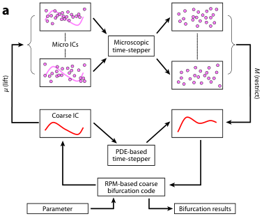
Chiavazzo2017 extended this approach to exploring the slow manifold, rather than just one trajectory. fig. 27 illustrates the idea in general: that projective integration may underpin analysis of the effective macroscale closure. The figure also displays the possibility of parallel micro-scale simulations, from various liftings (as in ensemble simulations of weather given finite measurements), in order to better estimate subsequent macro-state variables.
Bifurcation analysis
Gear02 discussed how given a macro-state, the process of lifting, a micro-burst, then restriction (and a backward micro-time projection) results in a macro-state that we view as a map .
- •
Then find macro-equilibria by solving numerically .
- •
Determine macroscale stability, independent of microscale chaos, from the Jacobian obtained by numerically differentiating .
- •
Continuation algorithms then fill-out a bifurcation picture for the macro-variables.
One could also determine macro-state limit cycles by applying projective integration and seeking a period that repeats the macro-state. Applications include modelling diseases Cisternas03, biological dispersal Erban2006, financial agents Siettos2012.
Further, one could find similarity solutions by setting up equations to seek steady states of a system when space-time-state variables are scaled somehow over some small time (Chen2004, e.g.).
For example, my script selfSim.m uses 10,000 random walking particles to simulate diffusion on a heterogeneous period-two lattice, and then rescaled short bursts iterate to the homogenised Gaussian distribution.
4.5 Open problems
- •
Develop projective integration when the microscale has high frequency oscillations—homogenise over time: e.g., the dichotomy is .
- •
Further, develop such time-homogenisation to systems which are stochastic on micro-times—crucial.
- •
Implement in the toolbox more general lifting and restricting operations.
- •
But now the ‘baby-bathwater’ question: what are appropriate macroscale variables?—after all we do not know the macroscale closure. For example, Young01 found that Brownian Bugs should not just be modelled by densities, but also needed to model the pair correlations in order to form a qualitatively correct closure. The challenge is to identify (dynamically?) all of the ‘baby’ before throwing out the ‘bathwater’.
- •
Implement ‘telescoping’ (recursive/many-level) projective integration (Gear03c, e.g.).
- •
Interface the toolbox to systems analysis tools such as auto.
5 Workshop: using the Equation-free Toolbox
Contents
This suite of Matlab/Octave functions empower users to start using the patch scheme and projective integration. Download the current version from GitHub. 1111 11 https://github.com/uoa1184615/EquationFreeGit.git
Many of the main functions, if invoked with no arguments, will execute a basic example.
For example, executing configPatches1 draws fig. 12 arising by simulating Burgers’ pde within eight patches.
Whereas executing configPatches2 computes a movie of the 2D nonlinear diffusion on a array of patches.
The aim of the workshop is for you to implement some example of interest to you. Some possibilities may be inspired by examples already discussed, or the following.
5.1 Patches in one spatial dimension
The user has to drive two functions in the toolbox: configPatches1 and patchSmooth1.
The first helps configure the patch scheme, whereas the second provides a function to be integrated in time, or stepped in time.
We have so far designed the toolbox so that the microscale quantities are defined on a microscale lattice (although, …).
In that scenario we need to create a multiscale grid in the space dimension, called x (a component of the struct patches).
Thus the configPatches1 function creates a 2D array x such that is the th microscale grid point in the th patch.
To create this multiscale grid the user must specify: the macroscale domain, Xlim such as ; the number of equi-spaced patches, nPatch say; the order of macroscale interpolation, here zero requests spectral; the (odd) number of microscale lattice points in each patch, nSubP say; and the patch micro/macro-scale ratio, here, equal to the patch half-width divided by the inter-patch spacing.
1 configPatches1(@BurgersPDE,[0 2*pi] ... 2 ,nan,8,0,0.2,7);
Then a user may specify an initial condition for a simulation simply by computing an expression for all entries in patches.x : for example,
1 u0=0.3*(1+sin(patches.x)) ... 2 +0.1*randn(size(patches.x));
During a simulation, the function patchSmooth1 computes the patch edge-values by macroscale interpolation of the patch centre-values.
The implemented order of the interpolation is specified in ordCC: is nearest neighbour quadratic; additionally involves the next-nearest neighbours in quartic interpolation; and so on—except that ordCC=0 is spectral interpolation.
How many edge-values are interpolated?
At least one on each edge, but if a user’s microscale system is ‘higher-order’ then it may need two or more microscale lattice edge points interpolated at each edge.
Specifying nEdge allows this (the default is one).
The last thing that the patch scheme needs, and the first in the parameter list for configPatches1, is the name of a user’s function that computes microscale time derivatives/steps (such as the following).
Example of Burgers PDE inside patches
As a microscale discretisation of Burgers’ pde , here code .
1 function ut=BurgersPDE(t,u,x) 2 dx=diff(x(1:2)); % microscale spacing 3 i=2:size(u,1)-1; % inside patches 4 ut=nan(size(u)); % 2D storage 5 ut(i,:)=diff(u,2)/dx^2 ... 6 -30*u(i,:).*(u(i+1,:)-u(i-1,:))/(2*dx); 7 end
General code overview
- 1.
invoke
configPatches1()and other initialisation - 2.
user time loop/integration, e.g.
ode15s- (a)
invoke
patchSmooth1()- i.
patchEdgeInt1()computes edge values - ii.
user function for time step/derivative, e.g.
BurgersPDE()
- i.
- (a)
- 3.
process results
1 [ts,ucts] = ode15s(@patchSmooth1 ... 2 ,[0 0.5],u0(:));
Suppose processing the results is to draw some graphs of the simulation,
and suppose the simulation is [ts,us]=ode15s(patchSmooth1,...).
The patches are most easily seen by breaking the plots between patches, as in fig. 12: these breaks are most easily done by assigning nan to the -coordinates of the patch edges:
patches.x([1 end],:)=nan;
- •
Then
plot(patches.x(:),us(j,:)’)graphs the shape of the field at time , - •
or
surf(ts,patches.x(:),us’)graphs a surface over all times (as in fig. 12).
Reduce the patch size by choosing a smaller ratio and see that the macroscale predictions are essentially the same. Increase the number of points within each patch and see essentially the same. Increase the number of patches and see the increased macroscale resolution.
[reaction-diffusion pde] Change the microscale code to solve the reaction-diffusion Ginzburg–Landau pde . Use initial conditions which involve both positive and negative values of and see the predicted macroscale evolves to field being separated by transitions that may be relatively poorly resolved on the macroscale.
Multiple interacting components
Further, for systems with multiple components, such as a wave system and , then the microscale array u must be a 3D array whose third dimension has the size of the number of field variables at each microscale grid-point—generally determined from the user supplied initial conditions.
5.2 Simulate waves on multiscale staggered grids
The script waterWaveExample simulates both a linear ideal wave (fig. 28), and a nonlinear shallow water wave model in 1D.
To simulate the microscale detail of the waves we implement a staggered micro-grid.
Then a staggered grid of patches Cao2014a empowers macroscale predictions of floods and tsunamis.
The approach developed here applies to any wave-like system in the form
| (24) |
where the brackets indicate that the two nonlinear functions and may involve various spatial derivatives of the fields and .
For wave systems, a staggered grid is best. Let for microscale spacing , and grid values and for index odd/even respectively. Then we would code
Let’s implement both a staggered microscale grid and also staggered macroscale patches. As before define for microscale spacing and macroscale spacing , and grid values and for index odd/even respectively. Then the microscale odes are
With this definition, the centre-value () of the patches alternates between and values; that is, odd are -patches, and even are -patches. Hence the patches are staggered.
The user’s microscale code might be as in idealWavePDE.m (a little wasteful?)
1 function Ut = idealWavePDE(t,U,x) 2 global patches 3 dx = diff(x(2:3)); 4 Ut = nan(size(U)); ht = Ut; 5 i = 2:size(U,1)-1; 6 ht(i,:) = -(U(i+1,:)-U(i-1,:))/(2*dx); 7 Ut(i,:) = -(U(i+1,:)-U(i-1,:))/(2*dx); 8 Ut(patches.hPts) = ht(patches.hPts); 9 end
The patch/gap-tooth scheme:
- 1.
configPatches1, and add micro-information
- 2.
ode15s patchSmooth1 idealWavePDE
- 3.
process results
Establish the global data struct patches for the
pdes eq. 24 (linearised) solved on
-periodic domain, with eight patches, each patch of
half-size ratio , with eleven micro-grid points
within each patch, and spectral interpolation () of
‘staggered’ macroscale patches to provide the edge-values of
the inter-patch coupling conditions.
1 global patches 2 nPatch = 8 3 ratio = 0.2 4 nSubP = 11 %of the form 4*n-1 5 Len = 2*pi; 6 configPatches1(@idealWavePDE,[0 Len] ... 7 ,nan,nPatch,-1,ratio,nSubP);When the ‘order of interpolation’ is odd, here , then our patch scheme interpolates the centre-values of the even patches to provide the edge-values of the odd patches, and vice-versa.
Identify and store which micro-grid points are or values on the staggered micro-grid.
1 uPts = mod( (1:nSubP)’+(1:nPatch) ,2); 2 hPts = find(uPts==0); 3 uPts = find(uPts==1); 4 patches.hPts = hPts; 5 patches.uPts = uPts;
Set an initial condition of some progressive wave, with noise, into U.
1 U0 = nan(nSubP,nPatch); 2 U0(hPts) = 1+0.5*sin(patches.x(hPts)); 3 U0(uPts) = 0+0.5*sin(patches.x(uPts)); 4 U0 = U0+0.02*randn(nSubP,nPatch);
Using ode15s we then subsample the
results because micro-grid scale waves do not dissipate and
so even ode15s takes very small time-steps for all time—we need projective integration here.
1 [ts,Ucts]=ode15s(@patchSmooth1,[0 4],U0(:)); 2 ts = ts(1:5:end); 3 Ucts = Ucts(1:5:end,:);
Plot the simulation (fig. 28), setting nans to separate patches.
1 xs = patches.x; xs([1 end],:) = nan; 2 mesh(ts,xs(hPts),Ucts(:,hPts)’),hold on 3 mesh(ts,xs(uPts),Ucts(:,uPts)’),hold off 4 xlabel(’time t’), ylabel(’space x’) 5 zlabel(’u(x,t) and h(x,t)’)
Reduce the patch size by choosing a smaller ratio and see that the macroscale predictions are essentially the same. Increase the number of points within each patch and see essentially the same. Increase the number of patches and see the increased macroscale resolution.
[microscale viscosity in the wave] Change the microscale code to include viscous drag in the pde: modify to for some small . Rerun and choose to see the sub-patch microscale waves effectively damped, but the macroscale waves propagating largely unaffected.
5.3 Patches of nonlinear diffusion in two space dimensions
Similar to 1D, you have to drive two functions in the toolbox: configPatches2 and patchSmooth2.
The first helps configure the 2D patch scheme, whereas the second provides a function to be integrated or stepped in time.
To define 2D microscale quantities on a 2D array of patches we need to create a multiscale grid in the two space dimension (fig. 29), stored in x,y (two components of the struct patches).
The configPatches2 function creates two 2D arrays x,y such that is the th microscale grid point in the th patch.
To create this multiscale grid the user must specify the 2D macroscale domain in the four elements of , the number of equi-spaced patches in each direction in the two elements of nPatch, the (odd) number of microscale lattice points in each patch, nSubP, and the patch micro/macro-scale ratio has two elements giving the patch half-width divided by the inter-patch spacing in each direction.
In many parameters, if the supplied parameter is a scalar, then that scalar is set for both directions.
Then a user may specify an initial condition for a simulation by computing an expression for all entries in patches.xpatches.y.
But a complication is that the microscale computation is done on a 4D array of the field at —the th microscale grid point in the th patch.1212
12
The reason for this subscript ordering is the thought that it should be easier to parallelise over the patches.
So the coordinate arrays have to be rearranged into the 1st and 3rd, and the 2nd and 4th dimensions:
1 x = reshape(patches.x,nSubP,1,[],1); 2 y = reshape(patches.y,1,nSubP,1,[]);Then auto-replication of the x,y arrays empowers simple assignments such as (fig. 29)
1 u0 = exp(-x.^2-y.^2);
During a simulation, the function patchSmooth2 computes the patch edge-values by macroscale interpolation of the patch centre-values.
The implemented order of the interpolation is specified in ordCC as in 1D, and nEdge may specify that wider edge values are computed by the interpolation.
The last thing that the patch scheme needs, and the first in the parameter list for configPatches2, is the name of a user’s function that computes microscale time derivatives/steps (such as the following).
Example of nonlinear diffusion PDE inside patches
As a microscale discretisation of , code .
1 function ut = nonDiffPDE(t,u,x,y) 2 dx=diff(x(1:2)); dy=diff(y(1:2)); 3 i=2:size(u,1)-1; j=2:size(u,2)-1; 4 ut=nan(size(u)); % preallocate 5 ut(i,j,:,:)=diff(u(:,j,:,:).^3,2,1)/dx^2 ... 6 +diff(u(i,:,:,:).^3,2,2)/dy^2; 7 end
General code overview
- 1.
configPatches2()and other initialisation - 2.
user time loop/integration, e.g.
ode15s- (a)
invoke
patchSmooth2()- i.
patchEdgeInt2()computes edge values - ii.
user function for time step/derivative, e.g.
nonDiffPDE
- i.
- (a)
- 3.
process results
Suppose the simulation is via [ts,us]=ode15s(patchSmooth2,...), and let’s draw some graphs.
To graph the solution at any time :
- 1.
u=patchEdgeInt2(us(i,:));converts the th row ofusinto a 4D array via the interpolation, - 2.
then graph the macroscale, patch-centre, values with
1 mesh(x((1+end)/2,1,:,1), ... 2 ,y(1,(1+end)/2,1,:) ... 3 ,u((1+end)/2,(1+end)/2,:,:))
The patches are most easily seen by breaking a surface graph between patches, as in fig. 29:
- 1.
x([1 end],:,:,:)=nan;andy(:,[1 end],:,:)=nan;, by assigningnanto the -coordinates of the patch edges, breaks the graphed surface; - 2.
u=permute(u,[1 3 2 4]);then permutes the 4D array to separate the -direction in the first two indices, and the -direction in the last two; - 3.
u=reshape(u,[numel(x) numel(y)]);forms a 2D array with all the in the first index, and all the in the second; - 4.
surf(x(:),y(:),u’)graphs the patchy surface (as in fig. 29).
[Example of 2D waves]
For , the script wave2D, with function wavePDE, tests and simulates the simple wave PDE in 2D space: via the two component system and .
- •
Execute and see the pure-wave nature in the pure-imaginary eigenvalues, and the wave nature in the simulation.
- •
See the same macroscale simulation with smaller patches.
- •
Include some dissipation in the ‘momentum’ pde (but remove the eigenvalue
returninwave2Dscript:- –
say some simple drag ;
- –
then some viscous dissipation for small .
- –
When the viscous dissipation works for you, try an initial condition with microscale noise and see in the simulation the rapid decay of the sub-patch microscale waves.
5.4 Weave documentation in the toolbox
To create and document the various functions, we adapt an idea due to Neil D. Lawrence of the University of Sheffield.
The idea is to use block comments in Matlab and an environment in LaTeX in order to interleave Matlab/Octave code, and its documentation in LaTeX.
Each function is stored in a *.m file and has the following plan.
1 % Short explanation for "help fun" 2 % Author, date 3 %{ 4 \section{...} 5 Overview LaTeX explanation. 6 \begin{matlab} 7 %} 8 function ... 9 %{ 10 \end{matlab} 11 \paragraph{Input} ... 12 \paragraph{Output} ... 13 Repeated as desired: 14 LaTeX in end-matlab to begin-matlab 15 \begin{matlab} 16 %} 17 Matlab code between %} and %{ 18 %{ 19 \end{matlab} 20 Concluding LaTeX before last line. 21 %}The function code and documentation is included by \input{*.m} in a LaTeX source file.
We need to define the environment matlab to be some verbatim listing. There are many available. But fancyvrb does a good straightforward and flexible job.
\usepackage{fancyvrb}\newenvironment{matlab}% {\Verbatim[numbers=left ,firstnumber=\the\inputlineno]}% {\endVerbatim}Optionally, we get fancyvrb to omit the block comment pairs %{ and %},
although the following requires that the block comment pairs always be used.
\makeatletter\def\fancyvrbStartStop{% \edef\FancyVerbStartString {\@percentchar\@charrb} \edef\FancyVerbStopString {\@percentchar\@charlb} }\makeatother
Contributing to the toolbox
Draft a function and example(s) as in the style of the toolbox—see the Full Developer’s Manual (Appendix B) for more detail. Contact me.
Appendix A Computer algebra codes cited in text
Contents
These are written in Reduce, a powerful, fast and free computer algebra package [http://www.reduce-algebra.com/].
A.1 homoDiff.txt
1 Comment Homogenise period two diffusion. Order 40
2 construction finds the 1-3 case converges for
3 wavenumbers<2.5. AJR, 23 May 2019;
4 on div; off allfac; on revpri; factor df;
5
6 maxo:=4;
7 a:=am+ad; b:=am-ad;
8 % maxo:=20; am:=2; ad:=-1; % optional high-order case
9
10 depend uu,x,t;
11 let df(uu,t)=>duudt;
12 u1:=u2:=uu; duudt:=0;
13
14 let df(uu,x,~p)=>0 when numberp(p) and p>maxo;
15 for iter:=1:99 do begin
16 write res1:=-df(u1,t)
17 +a*(-u1+for k:=0:maxo sum df(u2,x,k)/factorial(k))
18 +b*(-u1+for k:=0:maxo sum df(u2,x,k)/factorial(k)*(-1)^k);
19 write res2:=-df(u2,t)
20 +b*(-u2+for k:=0:maxo sum df(u1,x,k)/factorial(k))
21 +a*(-u2+for k:=0:maxo sum df(u1,x,k)/factorial(k)*(-1)^k);
22
23 duudt:=duudt+(duudtd:=(res1+res2)/2);
24 u1:=u1+(u1d:=(res1-duudtd)/am/4);
25 u2:=u2-u1d;
26
27 if {res1,res2}={0,0} then write iter:=iter+10000;
28 end;
29
30 u1:=u1;
31 u2:=u2;
32 duudt:=duudt;
33 if maxo>10 then begin
34 on rounded; let df(uu,x,~p)=>z^(p/2); on list;
35 write coeff(duudt,z);
36 end;
37 end;
A.2 homoVibr.txt
1 Comment homogenise lattice vibration problem. For this
2 linear problem it appears that the resultant slow manifold
3 is exactly the same with just df(uu,t) changed to df(u,t,t)
4 in the evolution. AJR, 25 May 2019;
5 on div; off allfac; on revpri; factor df,uu,vv;
6
7 maxo:=4;
8 a:=am+ad; b:=am-ad;
9
10 depend vv,x,t; let df(vv,t)=>dvvdt;
11 depend uu,x,t; let df(uu,t)=>vv;
12 u1:=u2:=uu; dvvdt:=0;
13
14 let df(uu,x,~p)=>0 when numberp(p) and p>maxo;
15 for it:=1:9 do begin
16
17 v1:=df(u1,t); v2:=df(u2,t);
18 write res1:=-df(v1,t)
19 +a*(-u1+for k:=0:maxo sum df(u2,x,k)/factorial(k))
20 +b*(-u1+for k:=0:maxo sum df(u2,x,k)/factorial(k)*(-1)^k);
21 write res2:=-df(v2,t)
22 +b*(-u2+for k:=0:maxo sum df(u1,x,k)/factorial(k))
23 +a*(-u2+for k:=0:maxo sum df(u1,x,k)/factorial(k)*(-1)^k);
24
25 dvvdt:=dvvdt+(res1+res2)/2;
26 u1:=u1+(u1d:=(res1-res2)/8/am);
27 u2:=u2-u1d;
28 if {res1,res2}={0,0} then write it:=it+10000;
29 end;
30
31 u1:=u1;
32 u2:=u2;
33 dvvdt:=dvvdt;
34 end;
A.3 onePatchHomo.txt
1 Comment effective homogenisation closure of one patch of
2 two-periodic heterogeneous diffusion. The diffusivities are
3 a and b, alternating. The microscale spacing is d. Find
4 that if the patch half-size n is even, then we get the
5 correct coefficient of the homogenisation closure.
6 AJR, 27 Mar 2019 -- 27 May 2019;
7
8 procedure uint(x); 1-x^2; % for Dirchlet zero bdry at |x|=1
9 %procedure uint(x); 1-2/3*x-1/3*x^2; % for insulated bdry at x=-1
10
11 n:=2; % use dynamics of 2n-1 microgrid points inside the patch
12 nn:=2*n-1;
13 % Create linear operator
14 matrix ll(nn,nn),id(nn,nn);
15 for i:=1:nn do id(i,i):=1;
16 for i:=1:nn do ll(i,i):=-(a+b)/d^2;
17 for i:=1:nn-1 do ll(i,i+1):=ll(i+1,i):=
18 (if evenp(i) then b else a)/d^2;
19 ll(1,n):=ll(1,n)+b*uint(-n*d)/d^2$
20 ll(nn,n):=ll(nn,n)+a*uint(n*d)/d^2$
21 lldsq:=ll*d^2;
22
23 % eval lambda=mu/d^2; find eqn for small one
24 charpoly:=factorize(det(ll*d^2-mu*id));
25 for j:=1:length(charpoly) do begin
26 eqn:=part(charpoly,j,1);
27 if sub({mu=0,d=0},eqn)=0 then write "found ",j:=j+10000;
28 end;
29 eqn:=eqn;
30 % two iterations to asymptotically solve and test
31 jac:=sub({mu=0,d=0},df(eqn,mu))$
32 let d^4=>0; % order of error
33 mu:=0$ res:=eqn$
34 mu:=mu-res/jac; res:=eqn;
35 effDiffCoeff:=mu/d^2/sub(x=0,df(uint(x),x,x));
36
37 end;