Efficient Approximation Algorithms for Adaptive Seed MinimizationNote: A short version of the paper appeared in 2019 International Conference on Management of Data (SIGMOD ’19), June 30–July 5, 2019, Amsterdam, Netherlands. ACM, New York, NY, USA, 18 pages. https://doi.org/10.1145/3299869.3319881CCS: Information systems Data miningCCS: Information systems Social advertisingCCS: Information systems Social networksCCS: Theory of computation Probabilistic computationCCS: Theory of computation Submodular optimization and polymatroids

Let $G$ be a social network with a node set $V$ and a directed edge set $E$, where $|V|=n$ and $|E|=m$. For any edge $\langle u,v\rangle\in E$, we refer to $u$ as an incoming neighbor of $v$, and $v$ as an outgoing neighbor of $u$. Each edge $e=\langle u,v\rangle$ is associated with a propagation probability $p(e)\in(0,1]$. We refer to such a social network as a probabilistic social network.

Given a node set $S\subseteq V$, the influence propagation initiated by $S$ under the independent cascade (IC) model (Kempe et al. 2003) is modeled as a discrete-time stochastic process as follows. At time slot $t_{0}$ (the subscript indicates the index of the time slot), all nodes in $S$ are activated while all other nodes are inactive. Suppose that node $u$ is first activated at slot $t_{i}$, then $u$ has one chance to activate each outgoing neighbor $v$ with the probability $p(u,v)$ at slot $t_{i+1}$, after which $u$ remains active. This influence propagation process continues until no more inactive nodes can be activated. As to the linear threshold (LT) model, it demands that for each node $v\in G$, the propagation probabilities of all edges ending at $v$ sum up to no more than $1$. With a given node set $S$, LT model works in a similar discrete-time stochastic procedure as follows. At time slot $t_{0}$, each node $v\in G$ is assigned with a threshold $\lambda_{v}$ sampled uniformly from $[0,1]$, and only nodes in $S$ are activated. At time slot $t_{i}$, we check all inactive node $u$ of its incoming edges from activated neighbors that if the sum of their propagation probabilities is no smaller than $\lambda_{u}$. If it is, then $u$ is activated; otherwise $u$ remains inactive. This influence propagation process terminates once there is no further node activated. Let $I(S)$ be the total number of active nodes in $G$ when the influence propagation terminates. We refer to $S$ as the seed set, and $I(S)$ as the spread of $S$.

Alternatively, the influence propagation process can also be described by the live edge procedure (Kempe et al. 2003). Specifically, for each edge $e\in E$, we independently flip a coin of head probability $p(e)$ to decide whether the edge $e$ is live or blocked to generate a sample of influence propagation. All the blocked edges are removed and the remaining graph is referred to as a realization of the probabilistic social network $G$, denoted as $\phi$. Note that there are $2^{m}$ distinct possible realizations. Let $\Omega$ be the set of all possible realizations (i.e., the sample space) such that $\lvert\Omega\rvert=2^{m}$, and $\Phi\sim\Omega$ denote that $\Phi$ is a realization randomly sampled from $\Omega$. Given a realization $\phi\in\Omega$, the spread of any seed set $S\subseteq V$ under $\phi$ is the total number of nodes that are reachable from $S$, denoted as $I_{\phi}(S)$. Thus, for any seed set $S$, its expected spread $\mathbb{E}[I(S)]$ is defined as

where $p(\phi)$ is the probability for realization $\phi$ to occur. In other words, the expected spread of $S$ is the (weighted) average spread over all the realizations in $\Omega$.

Given a probabilistic social network $G=(V,E)$ and a threshold $\eta\in[1,n]$, the seed minimization problem aims to select a minimum number of seed nodes to influence at least $\eta$ nodes. In the conventional “non-adaptive” setting, seed minimization requires selecting a node set $S$ such that $\mathbb{E}[I(S)]\geq\eta$, without any knowledge of realization that would occur in the actual influence propagation process. As a consequence, the selected $S$ may influence fewer than $\eta$ nodes for some realizations or much more than $\eta$ nodes for some other realizations, both of which are undesirable scenarios.

Meanwhile, the adaptive strategy (i.e., a recursive select-observe-select procedure) has been shown to be more effective than the non-adaptive (i.e., just select based on model) strategy in many real-world applications (Asadpour et al. 2008; Chen and Krause 2013; Chen et al. 2014). Specifically, an adaptive strategy first selects a node $u$ from graph $G$, and then observes the set of nodes activated by choosing node $u$ as a seed node. Based on this observation, the strategy would choose the next node as one that could influence as many currently inactive nodes as possible. This procedure is carried out in an recursive manner, until at least $\eta$ active nodes are observed.

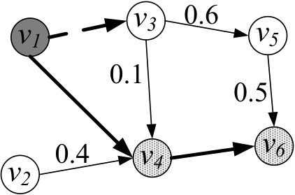
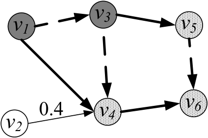
Figure 1 illustrates the adaptive strategy. Figures 1(a) and 1(b) show a social graph $G$ and one possible realization $\phi$ of $G$, respectively. Let $\eta=4$ and $\phi$ be the actual realization of influence propagation (which is unknown apriori). Figure 1(c) indicates that we first select node $v_{1}$ (in dark gray) as a seed node. Note that node $v_{1}$ influences nodes $v_{4}$ and $v_{6}$ (in light gray), with each bold (resp. dashed) arrow denoting a successful (resp. failed) step of influence. In addition, the thin arrows in Figures 1(c)–1(d) correspond to influence attempts which are not yet revealed. Since the number of nodes influenced by $v_{1}$ is less than $\eta$, we continue to select the second seed node. Figure 1(d) shows that we select $v_{3}$, which results in a total of $5$ active nodes, reaching the threshold $\eta$. Then, the adaptive seed selection process terminates.

In this paper, we aim to study seed selection strategies (referred to as policies) for adaptive seed minimization (ASM), which is formally defined as follows:

Note that when the propagation probability of every edge in $G$ is $1$, ASM reduces to the deterministic version of seed minimization, which is shown to be NP-hard (Goyal et al. 2013). Therefore, finding an optimal policy for ASM is also NP-hard.

Note that, in ASM, the influence spread in excess of the threshold $\eta$ has no value. Accordingly, we introduce the notion of truncated influence spread as follows.

Recall that ASM requires considering the influence spreads of nodes when the actual influence of some other nodes has been observed. Therefore, we also introduce the notion of marginal truncated influence spread as follows. Let $V_{1}=V$ and $G_{1}=G$. Let $V_{i}$ be the subset of nodes that remain inactive after round $(i-1)$, $G_{i}$ be the subgraph of $G$ induced by $V_{i}$. We refer to $G_{i}$ as the $i$-th residual graph. For example, in Figure 1, after round $1$, only nodes $v_{2},v_{3},v_{5}$ remain inactive, so $V_{2}=\{v_{2},v_{3},v_{5}\}$ and $G_{2}=(V_{2},E_{2})$ denotes the induced subgraph containing the thin edge $\langle v_{3},v_{5}\rangle$.

Let $S_{i}$ be the set of nodes selected as seeds by a policy in the first $i$ rounds. Similar to the definition of $\Omega$, we denote $\Omega_{i}$ as the set of all possible realizations in the $i$-th round. Then, for a node set $S\subseteq V_{i}$, we define the marginal spread $I_{\phi}(S\mid S_{i-1})$ as the additional spread that $S$ provides on top of $S_{i-1}$ under realization $\phi\in\Omega_{i}$, and define truncated marginal spread $\Gamma_{\phi}(S\mid S_{i-1})$ accordingly, i.e.,

Note that $I_{\phi}(S\mid S_{i-1})$ is exactly the influence spread of $S$ in the residual graph $G_{i}$ under realization $\phi$.

Let $n_{i}=\lvert V_{i}\rvert$ be the number of nodes in $G_{i}$, i.e.,  $I_{\phi}(S_{i-1})=n-n_{i}$ nodes have been activated by the end of round $i-1$, based on the partial realization revealed so far. Define $\eta_{i}=\eta-(n-n_{i})$. This is the amount by which the policy falls short of the target $\eta$ in the beginning of round $i$. Before reaching the threshold $\eta$, i.e., $\Gamma_{\phi}(S_{i-1})=I_{\phi}(S_{i-1})<\eta$, we can rewrite $\Gamma_{\phi}(S\mid S_{i-1})$ as

Then, $\Gamma_{\phi}(S\mid S_{i-1})$ can be easily computed in the residual graph $G_{i}$. For brevity, we define $\Gamma_{\phi}(v\mid S_{i-1}):=\Gamma_{\phi}(\{v\}\mid S_{i-1})$ for a singleton node set $\{v\}$.

Finally, we define the expected marginal truncated spread $\Delta(v\mid S_{i-1})$ as

In other words, the expected marginal truncated spread of a node $v$ is defined based on the “lift” in the expected number of active nodes that $v$ brings on top of previously selected seeds, over all realizations consistent with what has been observed in previous rounds.

Golovin and Krause (Golovin and Krause 2017) study the adaptive stochastic minimum cost coverage problem, which can be regarded as a variant of ASM in the case where there exists an oracle that accurately reports the expected marginal truncated spread for any given seed set. They propose to adopt a greed policy as follows. First, select the node $s_{1}$ with the largest expected truncated spread, i.e., $\Delta(s_{1}\mid S_{0})\geq\Delta(v\mid S_{0})$ for all $v\in V$. Then, observe the actual nodes that are activated by $s_{1}$ during the stochastic process, and remove them from $G$ to induce the residual graph $G_{2}$. After that, identify the node $s_{2}$ with the maximum expected marginal truncated spread $\Delta(s_{2}\mid S_{1})$ in the residual graph $G_{2}$. This process continues, such that each round selects the node with the largest expected marginal truncated spread, until we observe that no less than $\eta$ nodes have been influenced.

Golovin and Krause (Golovin and Krause 2017) show that the above greedy policy returns a $(\ln\eta+1)^{2}$-approximate solution to the optimum.¹¹ 1 Golovin and Krause claim that the approximation guarantee is $(\ln\eta+1)$ in an earlier version of their work (Golovin and Krause 2011), but point out that the proof has gaps in a revised version (Golovin and Krause 2017). Whether the logarithmic bound holds is an interesting open problem. This approximation guarantee, however, does not lead to a practical algorithm for the ASM problem, because (i) it requires the help from an oracle to exactly identify the node with the maximum expected marginal truncated spread in each round, but (ii) computing the exact expected spread of any node set is #P-hard (Chen et al. 2010a).

Motivated by this observation, Vaswani and Lakshmanan (Vaswani and Lakshmanan 2016) attempt to extend Golovin and Krause’s method by replacing the oracle with an spread estimator with bounded errors. In particular, they assume that for any node set $S$, the estimation ${\mathbb{E}}[\tilde{I}(v\mid S)]$ of the marginal gain $\mathbb{E}[I(v\mid S)]:=\mathbb{E}[I(S\cup\{v\})]-\mathbb{E}[I(S)]$ should satisfy

where ${\alpha^{\top}}/{\alpha^{\bot}}$ denotes the multiplicative error in calculating the marginal gains. Unfortunately, this requirement on the spread estimation is so stringent that no existing methods for influence estimation could fulfill the requirement without incurring prohibitive estimation overhead. To explain, suppose that the expected marginal spread $\mathbb{E}[I(v\mid S)]$ of a node $v$ on top of $S$ is small. In that case, Equation (7) would only allow a trivial amount of estimation error, which is rather difficult to achieve by existing methods for spread estimation.

In addition, the algorithm in (Vaswani and Lakshmanan 2016) attempts to select the node with the largest marginal spread in each round, instead of the node with the maximum marginal truncated spread. As a consequence, even when there exists an efficient estimator that provides highly accurate spread estimation, the algorithm in (Vaswani and Lakshmanan 2016) would still fail to achieve the type of approximation guarantee in (Golovin and Krause 2017), which the theoretical analysis in (Golovin and Krause 2017) is based on the notion of truncated spreads. We illustrate this issue with an example.

In recent work (Han et al. 2018), Han et al. study the problem of adaptive influence maximization, which also considers the adaptive setting, but aims to identify a predefined number of $k$ seed nodes that could influence the maximum number of users in $G$ in expectation. At the first glance, it may seem that we can modify the adaptive influence maximization algorithms to solve the adaptive seed minimization problem, in the same way that existing work (Goyal et al. 2013) transforms non-adaptive influence maximizing algorithms to address non-adaptive seed minimization. This approach, however, does not work because the algorithm in (Han et al. 2018) is designed based on vanilla expected marginal spreads. Instead, ASM requires considering truncated expected marginal spreads, as we previously discussed. As a consequence, the algorithm in (Han et al. 2018) cannot be adopted in our setting.

We propose a general framework, referred to as ASTI, to address the ASM problem. Algorithm 1 shows the details. Given a probabilistic social graph $G$ and a threshold $\eta$, ASTI aims to return a seed set $S$ such that $\Gamma(S)\geq\eta$, where $\Gamma(S)$ is the truncated influence spread of $S$ (i.e., the smaller one of the threshold $\eta$ and the number of active nodes influenced by $S$). In a nutshell, ASTI iteratively (i) selects the node to maximize the expected marginal truncated spread (Line 1), (ii) observes the newly influenced nodes (Line 1), and then (iii) updates the corresponding information (Lines 1–1). The process stops when at least $\eta$ nodes are activated (Line 1).

The key step of ASTI is truncated influence maximization that targets at identifying a node to maximize the expected marginal truncated spread (Line 1). If an $\alpha$-approximate solution for truncated influence maximization is obtained in each round (Line 1), ASTI provides a non-trivial approximation guarantee, as shown in the following theorem.

The proof²² 2 The formal proofs of all theoretical results are given in Appendix B. of Theorem 3.1 is based on adaptive submodular optimization (Golovin and Krause 2017). Theorem 3.1 requires that the policy should be an $\alpha$-approximate greedy one with respect to the expected marginal truncated spread $\Delta(v\mid S_{i-1})$. The challenge for designing such an $\alpha$-approximate greedy policy lies in how to develop a proper sampling method for estimating the truncated influence spread.

According to Theorem 3.1, in order to provide the theoretical guarantee, the algorithm is supposed to identify a node whose truncated marginal spread is an $\alpha$-approximation to the maximum truncated marginal spread in each round. At a first glance, it seems that we can utilize Borgs et al.’s reverse influence sampling method (Borgs et al. 2014). Unfortunately, in what follows, we show that Borgs et al.’s sampling method (Borgs et al. 2014) fails to estimate the truncated influence spread accurately.

Specifically, Borgs et al. (Borgs et al. 2014) propose to generate random reverse reachable (RR) sets for influence maximization. Compared with the Monte-Carlo simulation (Kempe et al. 2003), RR-sets can dramatically accelerate the seed selection process while retaining the same approximation guarantees for influence maximization (Borgs et al. 2014). In particular, a random RR-set of $G$ is generated by first selecting a node $v\in V$ uniformly at random, and then taking the nodes that can reach $v$ in a random realization. Evidently, a random RR-set is a subgraph of the corresponding random realization $\Phi$, which is generated by performing a reverse breadth first search (BFS) on $\Phi$ starting from the random node $v$. A random RR-set $R$ is an unbiased spread estimator, i.e., for any seed set $S$,

Unfortunately, RR-sets fail to estimate truncated influence spread accurately. Intuitively, the expectation of this estimator for truncated influence spread of $S$ is

Recall that the true expected truncated influence spread is

Obviously, for any $\phi\in\Omega$, unless $I_{\phi}(S)=n$,

Specifically, consider the case that $I_{\phi}(S)\leq\eta$ for all $\phi$. Then, this estimator is biased with a discount ${\eta}/{n}$, which is extremely inaccurate when $\eta\ll n$. In practice, $\eta$ is likely to be a fraction of $n$, since even a set of ten thousand seed nodes has been found to influence less than half population on many datasets (Nguyen et al. 2017). These facts indicate that RR-sets are highly biased for estimating truncated influence spread. As a consequence, the state-of-the-art algorithms (Huang et al. 2017; Nguyen et al. 2016; Tang et al. 2015; Tang et al. 2018b; Tang et al. 2014) for influence maximization that utilize RR-sets (Borgs et al. 2014) cannot provide theoretical guarantees for truncated influence maximization. In turn, this means that these algorithms cannot be fashioned to solve ASM with approximation guarantees. To address this issue, we propose a novel sampling approach that generates multi-root reverse reachable (mRR) sets which can estimate the truncated influence spread efficiently and effectively. The algorithm utilizing mRR-sets is referred to as TRIM ³³ 3 TRuncated Influence Maximization.. We rigorously show that TRIM can provide strong theoretical guarantees for truncated influence maximization and thus ASTI instantiated with TRIM is guaranteed to approximate ASM within a constant ratio.

If we generate $n$ correlated RR-sets such that (i) they start from $n$ distinct nodes, and (ii) the materialization of each edge is consistent in all the RR-sets, then merging these RR-sets (with duplicates removed) as well as the edge statuses forms a realization sample. Based on this observation, if we generate $k$ $(k<n)$ correlated RR-sets using the same rule, then merging them as a $k$-root RR-set is likely to estimate the truncated influence spread more accurately compared against a vanilla RR-set. To explain how multi-root reverse reachable (mRR) set works, we first introduce its definition.

By definition, the key difference between an mRR-set and an RR-set is that the former has multiple roots whereas the latter has one single root only. Similar to the generation of RR-sets, a random mRR-set can be generated by:

1. (1)

   Choose a set of $k$ nodes $K\subseteq V$ uniformly at random;

2. (2)

   Perform a stochastic reverse breadth first search (BFS) that starts from $K$ and follows the incoming edges of each node. Insert into $R$ all nodes that are traversed during the stochastic BFS.

A natural question is how to decide the size of $k$ for truncated spread estimation? The setting of $k$ yields a tradeoff between efficiency and accuracy in that a larger $k$ provides more accurate estimation but takes more computational resources. Through the aforementioned analysis of RR-set, we find that the high-efficiency of RR-set comes from its “binary” property. In particular, a random RR-set $R$ estimates the influence spread of any node set $S$ as $n$ if $R\cap S\neq 0$, and as $0$ otherwise. To avoid maintaining the edge statuses, our mRR-set estimator shall retain this binary property. That is, it estimates the truncated influence spread of $S$ as $\eta$ if and only if $S$ intersects this mRR-set, and as $0$ otherwise. For a given $k$-RR-set $R$, if a node $v\in R$, then $v$ can reach at least one of the $k$ starting nodes. Then, its influence spread is estimated to be at least $n/k$ and thus its estimated truncated influence spread is at least $\min\{n/k,\eta\}$. By setting $n/k\geq\eta$, the estimated truncated influence spread is $\eta$.

On the other hand, to improve the accuracy, $k$ should be set as large as possible. So we choose $k=n/\eta$. However, ${n}/{\eta}$ is not an integer in general. To address this issue, we adopt a randomized rounding approach. To generate a mRR-set, we randomly choose a set $K$ of nodes such that its size $k$ equals $\lfloor\frac{n}{\eta}\rfloor+1$ with probability $\frac{n}{\eta}-\lfloor\frac{n}{\eta}\rfloor$, and equals $\lfloor\frac{n}{\eta}\rfloor$ otherwise. Then, the expectation of $k$ is ${n}/{\eta}$. However, we note that when $k=\lfloor\frac{n}{\eta}\rfloor+1$, the possible value of the estimated truncated influence spread is no longer binary (i.e., $0$ or $\eta$). To address such a new challenge, we define an estimator $\tilde{\Gamma}(S)$ as $\tilde{\Gamma}(S)=\eta$ if and only if $S\cap R\neq\emptyset$, and $\tilde{\Gamma}(S)=0$ otherwise. At the first glance, it seems that the relationship between $\mathbb{E}[{\Gamma}(S)]$ and $\mathbb{E}[\tilde{\Gamma}(S)]$ is unclear. Fortunately, the following theorem shows that under the above setting of $k$ such that $\mathbb{E}[k]={n}/{\eta}$, the ratio of ${\mathbb{E}[\tilde{\Gamma}(S)]}$ and ${\mathbb{E}[{\Gamma}(S)]}$ is in the range of $[1-1/{\mathrm{e}},1]$.

Theorem 3.3 states that $\tilde{\Gamma}$ is a biased but sufficiently accurate estimator of the expected truncated influence spread $\mathbb{E}[\Gamma(S)]$. In fact, this estimator also works for any residual graph $G_{i}$. Specifically, let $\tilde{\Gamma}(S\mid S_{i-1})$ be the estimated truncated spread of $S$ in $G_{i}$ with respect to $\eta_{i}$, the lowered target corresponding to graph $G_{i}$. Recall that $\eta_{i}=\eta-(n-n_{i})$. We have the following corollary.

Now, we can construct a $(1-1/{\mathrm{e}})(1-\varepsilon)$-approximate greedy policy using the estimator $\tilde{\Gamma}$ built upon mRR-sets.

Algorithm 2 presents the details of TRIM that can return a $(1-1/{\mathrm{e}})(1-\varepsilon)$-approximate solution for truncated influence maximization for any input graph $G_{i}$ and error threshold $\varepsilon$. TRIM is similar in spirit to OPIM-C which is the state-of-the-art algorithm for influence maximization (Tang et al. 2018b). Specifically, OPIM-C uses two disjoint groups of random RR-sets, among which one group is used to derive the solution and the other is used to verify its quality. We customize TRIM by utilizing one group of mRR-sets, which would be more efficient for selecting a singleton seed set as pointed out in (Huang et al. 2017). In a nutshell, TRIM starts from a small number of mRR-sets and iteratively increases the mRR-set number until a satisfactory solution is identified. Next, we discuss the details of TRIM.

In the mRR-set sampling stage (Lines 2 and 2), each mRR-set is started from a random set $K$ of nodes whose size $k$ is an independent random number. Recall that $k$ is $\lfloor\frac{n_{i}}{\eta_{i}}\rfloor+1$ with probability $\frac{n_{i}}{\eta_{i}}-\lfloor\frac{n_{i}}{\eta_{i}}\rfloor$ and $\lfloor\frac{n_{i}}{\eta_{i}}\rfloor$ otherwise. Given a set $\mathcal{R}$ of random mRR-sets, we say that a node $v$ covers a mRR-set $R\in\mathcal{R}$ if $v\in R$, and we define the coverage of $v$ in $\mathcal{R}$, denoted as $\Lambda_{\mathcal{R}}(v)$, as the number of mRR-sets in $\mathcal{R}$ that are covered by $v$. Based on the mRR-sets generated, TRIM identifies the node $v^{\ast}\in V_{i}$ that covers the largest number of mRR-sets in $\mathcal{R}$ (Line 2). Let $v^{\circ}$ be the optimal node such that $\Delta(v^{\circ}\mid S_{i-1})=\max_{v\in V_{i}}\Delta(v\mid S_{i-1})$. Then, $\Lambda_{\mathcal{R}}(v^{\circ})$ is bounded by $\Lambda_{\mathcal{R}}(v^{\ast})$. According to Lemma A.2 in Appendix A, with high probability, $\Lambda^{l}(v^{\ast})$ (Line 2) is a lower bound on the expected coverage of $v^{\ast}$ in $\mathcal{R}$, which indicates that

Similarly, with high probability, $\Lambda^{u}(v^{\circ})$ (Line 2) is an upper bound on the expected coverage of $v^{\circ}$ in $\mathcal{R}$. Thus,

In addition, by Equation (11) in Corollary 3.4, we know that

Combining Equations (12)–(14), we can derive a quantitative relationship between $\Delta(v^{\ast}\mid S_{i-1})$ and $\Delta(v^{\circ}\mid S_{i-1})$ such that with high probability

Therefore, the final guarantee is $(1-1/{\mathrm{e}}){\Lambda^{l}(v^{\ast})}/{\Lambda^{u}(v^{\circ})}$. Note that in our stopping condition of ${\Lambda^{l}(v^{\ast})}/{\Lambda^{u}(v^{\circ})}\geq 1-\hat{\varepsilon}$ (Line 2), we use $\hat{\varepsilon}$ (defined in Line 2) to correct the error on Equations (12) and (13) (with low failure probability). This proves the $(1-1/{\mathrm{e}})(1-\varepsilon)$ approximation ratio of $\Delta(v^{\ast}\mid S_{i-1})$.

Before we proceed to the theoretical analysis, we first present the hardness of ASM.

Combining Theorem 3.1 and Lemma 3.6, we obtain the approximation guarantee of ASTI.

Now, we present the following lemma that gives the expected number of mRR-sets generated by TRIM. The proof is similar to that of OPIM-C (Tang et al. 2018b).

Finally, we provide the expected time complexity of TRIM in the following lemma.

At the first glance, the expected time complexity of TRIM is counterintuitive. In particular, the expected root size of $n_{i}/\eta_{i}$ in the $i$-th round is increasing with $i$. It seems that the time complexity of TRIM is more likely to increase with $i$. However, Lemma 3.10 just tells us the opposite. This is due to either the residual graph $G_{i}$ being reduced significantly (Lemma 3.8) or the mRR-set size being reduced considerably (Lemma 3.9). Overall, the time complexity of TRIM in each round can be independent of the number of initially selected nodes. There are at most $\eta$ rounds in total, we can derive the expected time complexity of ASTI instantiated with TRIM.