跳到论文正文
W Papers独立论文阅读器 arXiv:1907.09317 论文正文 计算阅读时间 · 0%
引用这篇论文根据当前论文元数据生成,正式投稿前建议核对。


License: arXiv.org perpetual non-exclusive license
arXiv:1907.09317v2 [math.PR] 13 Jul 2020

KPZ equation correlations in time

Ivan Corwin    Promit Ghosal    Alan Hammond

We consider the narrow wedge solution to the Kardar-Parisi-Zhang stochastic PDE under the characteristic 3:2:13:2:1 scaling of time, space and fluctuations. We study the correlation of fluctuations at two different times. We show that when the times are close to each other, the correlation approaches one at a power-law rate with exponent 2/32/3, while when the two times are remote from each other, the correlation tends to zero at a power-law rate with exponent −1/3-1/3. We also prove exponential-type tail bounds for differences of the solution at two space-time points.

Three main tools are pivotal to proving these results: 1) a representation for the two-time distribution in terms of two independent narrow wedge solutions; 2) the Brownian Gibbs property of the KPZ line ensemble; and 3) recently proved one-point tail bounds on the narrow wedge solution.

,  and

??Department of Mathematics, Columbia University, ??

??Department of Mathematics, Massachusetts Institute of Technology, ??

??Departments of Mathematics and Statistics, U.C. Berkeley, ??

1 Introduction

The Kardar-Parisi-Zhang stochastic PDE, written formally as

∂tℋ⁡(t,x)=12​∂x2ℋ⁡(t,x)+12​(∂xℋ⁡(t,x))2+ξ⁡(t,x),\displaystyle\partial_{t}\mathcal{H}(t,x)=\frac{1}{2}\partial^{2}_{x}\mathcal{H}(t,x)+\frac{1}{2}(\partial_{x}\mathcal{H}(t,x))^{2}+\xi(t,x)\,, (1)

governs the random evolution in time t≥0t\geq 0 of an interface ℋ⁡(t,⋅):ℝ→ℝ\mathcal{H}(t,\cdot):\mathbb{R}\to\mathbb{R}. The interface grows in the normal direction, while being smoothed by surface tension and roughened by a field of randomness that is independent between distinct space-time points – a field represented in the equation by the space-time Gaussian white noise ξ\xi. In the physically relevant Cole-Hopf solution, it is specified that ℋ⁡(t,x)=log⁡𝒵⁡(t,x)\mathcal{H}(t,x)=\log\mathcal{Z}(t,x), where 𝒵\mathcal{Z} is the solution to the stochastic heat equation (SHE)

∂t𝒵⁡(t,x)\displaystyle\partial_{t}\mathcal{Z}(t,x) =12​∂x2𝒵⁡(t,x)+ξ⁡(t,x)​𝒵​(t,x).\displaystyle=\frac{1}{2}\partial^{2}_{x}\mathcal{Z}(t,x)+\xi(t,x)\mathcal{Z}(t,x)\,. (2)

The fundamental solution to the SHE – to be denoted here by 𝒵𝐧𝐰​(t,x)\mathcal{Z}^{\mathbf{nw}}(t,x) – has initial data 𝒵⁡(0,x)\mathcal{Z}(0,x) set equal to a Dirac delta function δ⁡(x)\delta(x) at x=0x=0. In this article, we study the resulting narrow wedge solution to the KPZ equation, namely ℋ𝐧𝐰​(t,x)=log⁡𝒵𝐧𝐰​(t,x)\mathcal{H}^{\mathbf{nw}}(t,x)=\log\mathcal{Z}^{\mathbf{nw}}(t,x). The initial condition ℋ𝐧𝐰​(0,x)\mathcal{H}^{\mathbf{nw}}(0,x) is not well-defined; however, for small tt, ℋ𝐧𝐰​(t,x)\mathcal{H}^{\mathbf{nw}}(t,x) resembles the curve −x22​t-\tfrac{x^{2}}{2t}, so that the name ‘narrow wedge’ may be seen as a substitute for the informative but prosaic term ‘narrow parabola’.

The solution theory for the SHE is standard and is discussed in [63, 13]. The mathematical analysis of the KPZ equation has, however, offered many outstanding challenges: notably, for showing that the equation accurately approximates the evolution of physical growth processes; for developing a solution theory that is robust enough to permit such approximations; and for studying properties of the solution’s probability distribution and various asymptotics. Indeed, the Cole-Hopf KPZ solution has been shown in [9] to coincide with limits of certain discrete growth processes; while the development of solution theory has been the object of intense recent activity, including the theory of regularity structures [41]; energy solutions [37, 40]; paracontrolled distributions [38, 39]; and the renormalization group [52]. The reader may consult [24] for a discussion of recent advances in the theory of singular stochastic PDE. Our present investigation focusses on the third area of challenge – the properties of the KPZ equation’s probability distribution.

Since the work of Kardar, Parisi and Zhang [51], the KPZ equation has been predicted to behave non-trivially in its long-time limit under a 3:2:13:2:1 scaling of time, space and fluctuations. The 1/31/3 fluctuation exponent was first verified in [4] for stationary initial data; in [2], this exponent, and the corresponding limiting one-point distribution, was identified for narrow wedge initial data. The 2/32/3 spatial exponent was first verified in [20] for the narrow wedge.

The purpose of the present paper is to verify for the first time the KPZ equation’s 3/33/3 temporal exponent in the case of narrow wedge initial data. We will prove that the correlation of centred and scaled fluctuations at a pair of distinct moments in the time scale tt transitions between one as the times approach each other, and zero as they separate – and we will quantify this transition with precise power-law exponents for the speed.

First we specify notation that represents a 3:2:13:2:1 scaled version of ℋ𝐧𝐰​(t,x)\mathcal{H}^{\mathbf{nw}}(t,x) in a manner suitable for the presentation and proof of our main results. The parameter t>0t>0 specifies a time scale; the value of α>0\alpha>0 specifies time judged on this scale; and x∈ℝx\in\mathbb{R} specifies location judged on the suitable spatial scale t2/3t^{2/3}. Indeed, for t,α>0t,\alpha>0 and x∈ℝx\in\mathbb{R}, we set

𝔥t(α,x):=t−1/3(ℋ𝐧𝐰(αt,t2/3x)+αt/24).\displaystyle\mathfrak{h}_{t}(\alpha,x):=t^{-1/3}\Big(\mathcal{H}^{\mathbf{nw}}\big(\alpha t,t^{2/3}x\big)+\alpha t/24\Big)\,. (3)

The use of a pair (α,t)(\alpha,t) of temporal parameters may seem to introduce a touch of redundancy, but various scalings are in our view simplified by the use of these parameters; and we hope that conceptual clarity is offered by the division of roles between tt, whose value fixes a time scale, and α\alpha, which varies on the given scale.

1.1 Main results

Our first main result gives bounds on the correlation between 𝔥t​(1,0)\mathfrak{h}_{t}(1,0) and 𝔥t​(α,0)\mathfrak{h}_{t}(\alpha,0) for α>2\alpha>2. In this case of two remote times, correlations decay as α−1/3\alpha^{-1/3} in the limit of high α\alpha. Recall that the correlation between two random variables XX and YY is defined to be

Corr⁡(X,Y)=Cov⁡(X,Y)Var⁡(X)​Var⁡(Y),whereCov⁡(X,Y)=𝔼⁡[X​Y]−𝔼⁡[X]​𝔼​[Y].\mathrm{Corr}\big(X,Y\big)=\frac{\mathrm{Cov}\big(X,Y\big)}{\sqrt{\mathrm{Var}(X)}\sqrt{\mathrm{Var}(Y)}},\qquad\textrm{where}\qquad\mathrm{Cov}\big(X,Y\big)=\mathbb{E}[XY]-\mathbb{E}[X]\,\mathbb{E}[Y].
Theorem 1.1 (Remote correlations).

There exist t0,c1,c2>0t_{0},c_{1},c_{2}>0 such that, for all t>t0t>t_{0} and α>2\alpha>2,

c1α−1/3≤Corr(𝔥t(1,0),𝔥t(α,0))≤c2α−1/3.\displaystyle c_{1}\alpha^{-1/3}\leq\mathrm{Corr}\big(\mathfrak{h}_{t}(1,0),\mathfrak{h}_{t}(\alpha,0)\big)\leq c_{2}\alpha^{-1/3}\,. (4)

The second main result bounds the correlation between 𝔥t​(1,0)\mathfrak{h}_{t}(1,0) and 𝔥t​((β+1),0)\mathfrak{h}_{t}((\beta+1),0) when β\beta is smaller than 1/21/2. As β\beta approaches zero, the correlation between 𝔥t​(1,0)\mathfrak{h}_{t}(1,0) and 𝔥t​(β+1,0)\mathfrak{h}_{t}(\beta+1,0) approaches one with a discrepancy of order β2/3\beta^{2/3}.

Theorem 1.2 (Adjacent correlations).

For any t0>0t_{0}>0, there exist c1=c1​(t0)>0c_{1}=c_{1}(t_{0})>0 and c2=c2​(t0)>0c_{2}=c_{2}(t_{0})>0 such that, for all t>t0t>t_{0} and β∈(0,1/2)\beta\in(0,1/2) satisfying β​t>t0\beta t>t_{0},

c1​β2/3≤1−Corr⁡(𝔥t​(1,0),𝔥t​(1+β,0))≤c2​β2/3.\displaystyle c_{1}\beta^{2/3}\leq 1-\mathrm{Corr}\big(\mathfrak{h}_{t}(1,0),\mathfrak{h}_{t}(1+\beta,0)\big)\leq c_{2}\beta^{2/3}\,. (5)

These theorems invite a number of interesting questions. Notice that, in Theorem 1.1, the minimal time t0t_{0} must be large enough for the bounds to hold. First, we may ask: what happens to the two bounds for small tt? In fact, in our proof of this theorem, we show a stronger upper bound: for any t0>0t_{0}>0, there exists c2​(t0)>0c_{2}(t_{0})>0 so that, for all t>t0t>t_{0} and α>2\alpha>2, Corr⁡(𝔥t​(1,0),𝔥t​(α,0))\mathrm{Corr}\Big(\mathfrak{h}_{t}(1,0),\mathfrak{h}_{t}(\alpha,0)\Big) is at most c2α−1/3c_{2}\alpha^{-1/3}. Our proof does not, however, produce a matching lower bound. It is unclear to us if a new phenomenon occurs at short time that renders such a bound invalid or if instead our technique of proof is unsuitable for obtaining a bound of this form.

A second question also touches on short-time behaviour. In Theorem 1.2 we require β​t>t0\beta t>t_{0} for some arbitrary yet fixed t0t_{0}. For tt fixed, this limits us to values of β>t0/t\beta>t_{0}/t. (As t↗∞t\nearrow\infty, this lower bound tends to zero.) What happens for β\beta smaller than t0/tt_{0}/t? The source of the restriction β​t>t0\beta t>t_{0} comes from the application of the one-point tail behaviour from Propositions 2.11 and 2.12. These tail bounds are valid provided that time exceeds t0t_{0}. When the time gap β​t\beta t is less than t0t_{0}, we need short-time tail bounds which are presently not available in the literature. As we remark at the end of Section 1.3, this condition that β>t0/t\beta>t_{0}/t (as well as both of our main theorems) has an interpretation in terms of aging.

Finally, a third question concerns the specification of the constants c1c_{1} and c2c_{2} in Theorem 1.1 and 1.2. In the physics literature, de Nardis and Le Doussal [27, 28] provide various predictions concerning the two time distribution, in particular the constants. For instance, they claim that as α,t→∞\alpha,t\to\infty the correlation in Theorem 1.1 behaves like α−1/3\alpha^{-1/3} times a limiting constant written in terms of the Airy2 process 𝒜2​(⋅)\mathcal{A}_{2}(\cdot) and a two-sided Brownian motion B⁡(⋅)B(\cdot) as

limα→∞limt→∞α13​Corr​(𝔥t​(α,0),𝔥t​(1,0))=Corr⁡(𝒜2​(0),maxy⁡{𝒜2​(y)−y2+2​B​(y)})Var​(𝒜2​(0))\displaystyle\lim_{\alpha\to\infty}\lim_{t\to\infty}\alpha^{\frac{1}{3}}\mathrm{Corr}(\mathfrak{h}_{t}(\alpha,0),\mathfrak{h}_{t}(1,0))=\frac{\mathrm{Corr}\big(\mathcal{A}_{2}(0),\max_{y}\{\mathcal{A}_{2}(y)-y^{2}+\sqrt{2}B(y)\}\big)}{\mathrm{Var}\big(\mathcal{A}_{2}(0)\big)} (6)

They also predict that the conditional density of 𝔥t​(1+β,0)−𝔥t​(1,0)\mathfrak{h}_{t}(1+\beta,0)-\mathfrak{h}_{t}(1,0) given 𝔥t​(1,0)\mathfrak{h}_{t}(1,0) converge to the Baik-Rains distribution as tt goes to ∞\infty followed by β\beta tends to 00. From this prediction one sees that in this limit, the correlation in Theorem 1.2 should behave like β2/3\beta^{2/3} times a constant given by the ratio of the variances of Baik-Rains distribution and the Tracy-Widom distribution. We have not tried to optimize our methods to access these precise values of the constants, though it is certainly worth more study.

We further mention some other natural themes related to our first two main results. Theorems 1.1 and 1.2 both probe the two-time correlation when the spatial coordinate is zero. In this context, two space-time points lie along a space-time line of velocity zero emanating from the origin. In general, space-time lines of fixed velocity emanating from the origin are called characteristics; and, by trivial affine shifts – see Proposition 2.6 – our results imply the same correlation behaviour along such characteristics. On the other hand, we have not addressed what happens when, say, Corr⁡(𝔥t​(1,0),𝔥t​(α,x))\mathrm{Corr}\big(\mathfrak{h}_{t}(1,0),\mathfrak{h}_{t}(\alpha,x)\big) is considered for x≠0x\neq 0. This is a problem that may plausibly be addressed by the methods of the present article. That said, if the aim is to prove results concerning more general initial data than the narrow wedge for the KPZ equation, our methods will not be useful without significant further input. Indeed, as the proof sketch offered in Section 1.2 will explain, we rely upon a special property of narrow wedge initial data, namely its connection to the KPZ line ensemble and this ensemble’s Gibbs property; and this essential aspect is lacking when general initial data is considered.

We state two further theorems concerning local fluctuations of the KPZ equation in space and time.

Theorem 1.3.

For any t0>0t_{0}>0 there exist s0=s0​(t0)>0s_{0}=s_{0}(t_{0})>0 and c=c⁡(t0)>0c=c(t_{0})>0 such that for all x∈ℝx\in\mathbb{R}, t≥t0t\geq t_{0}, s≥s0s\geq s_{0}, and ϵ∈(0,1]\epsilon\in(0,1],

ℙ⁡(supz∈[x,x+ϵ]|𝔥t​(1,z)+z22−𝔥t​(1,x)−x22|≥s​ϵ1/2)≤exp⁡(−c​s3/2).\displaystyle\mathbb{P}\,\bigg(\,\sup_{z\in[x,x+\epsilon]}\Big|\mathfrak{h}_{t}(1,z)+\tfrac{z^{2}}{2}-\mathfrak{h}_{t}(1,x)-\tfrac{x^{2}}{2}\Big|\,\geq\,s\epsilon^{1/2}\,\bigg)\leq\exp\big(-cs^{3/2}\big)\,. (7)

This theorem gauges fluctuation of the parabolically shifted process 𝔥t​(1,x)+x22\mathfrak{h}_{t}(1,x)+\tfrac{x^{2}}{2} since, as we will recall in Proposition 2.6, this shift renders the process stationary in the xx variable. Before turning to our theorem concerning fluctuations in time, we state a corollary of the preceding result, which gives an estimate on the spatial modulus of continuity for 𝔥t\mathfrak{h}_{t}. The corollary holds uniformly in the limit of high tt, so that, when the result is allied with the one-point convergence that will be the subject of Proposition 2.6, we learn that the spatial process is tight and that any subsequential limit shares the Hölder continuity known for the finite tt processes.

Corollary 1.4.

For t0>0t_{0}>0 and any interval [a,b]⊂ℝ[a,b]\subset\mathbb{R}, define

𝒞:=supx1≠x2∈[a,b]|x1−x2|−12(log|b−a||x1−x2|)−2/3|𝔥t(1,x1)+x122−𝔥t(1,x2)−x222|.\displaystyle\mathcal{C}:=\sup_{x_{1}\neq x_{2}\in[a,b]}|x_{1}-x_{2}|^{-\frac{1}{2}}\Big(\log\frac{|b-a|}{|x_{1}-x_{2}|}\Big)^{-2/3}\Big|\mathfrak{h}_{t}(1,x_{1})+\tfrac{x_{1}^{2}}{2}-\mathfrak{h}_{t}(1,x_{2})-\tfrac{x_{2}^{2}}{2}\Big|\,. (8)

Then there exist s0=s0​(t0,|b−a|)>0s_{0}=s_{0}(t_{0},|b-a|)>0 and c=c⁡(t0,|b−a|)>0c=c(t_{0},|b-a|)>0 such that, for s≥s0s\geq s_{0} and t>t0t>t_{0},

ℙ⁡(𝒞>s)≤exp⁡(−c​s3/2).\mathbb{P}\big(\mathcal{C}>s\big)\leq\exp\big(-cs^{3/2}\big)\,.

Our last result concerns the upper and lower tails for the difference in fluctuations at two times. These tail bounds will be used in the proofs of Theorems 1.1 and 1.2.

Theorem 1.5.

For any t0>0t_{0}>0, there exist s0=s0​(t0)>0s_{0}=s_{0}(t_{0})>0, c1=c1​(t0)>0c_{1}=c_{1}(t_{0})>0, c2=c2​(t0)>0c_{2}=c_{2}(t_{0})>0 and c3=c3​(t0)>0c_{3}=c_{3}(t_{0})>0 such that, for s>s0s>s_{0}, t>t0t>t_{0} and β∈(0,1/2)\beta\in(0,1/2) for which t​β>t0t\beta>t_{0},

exp⁡(−c1​s3/2)≤ℙ⁡(𝔥t​(1+β,0)−𝔥t​(1,0)≥β1/3​s)\displaystyle\exp\big(-c_{1}s^{3/2}\big)\leq\mathbb{P}\Big(\mathfrak{h}_{t}(1+\beta,0)-\mathfrak{h}_{t}(1,0)\geq\beta^{1/3}s\Big) ≤exp⁡(−c2​s3/4),\displaystyle\leq\exp\big(-c_{2}s^{3/4}\big)\,, (9)
ℙ⁡(𝔥t​(1+β,0)−𝔥t​(1,0)≤−β1/3​s)\displaystyle\mathbb{P}\Big(\mathfrak{h}_{t}(1+\beta,0)-\mathfrak{h}_{t}(1,0)\leq-\beta^{1/3}s\Big) ≤exp⁡(−c3​s3/2).\displaystyle\leq\exp\big(-c_{3}s^{3/2}\big)\,. (10)

Just as in Theorem 1.2, we suspect different behaviour will arise in the short-time limit as β→0\beta\to 0 for tt fixed. Because of this lack of a short-time result, we do not present a temporal modulus of continuity result arising from this theorem in the style of the spatial Corollary 1.4. Notice, also, that we do not record a lower bound on the probability in (10); we have not pursued this since we presently have no application for it. Finally, although we focus here on x=0x=0 at both times, it should also be possible to address two different spatial locations.

1.2 Idea of proof

Before describing our methods, we explain why existing approaches to studying the KPZ equation do not yield our main results. The KPZ equation has attracted attention of specialists in stochastic PDE – via regularity structures, paracontrolled distributions or the renormalization group, for example – and of probabilists using integrable methods involving, for instance, Macdonald processes and the Bethe ansatz. It is natural enough to ask why our results do not follow from techniques in either of these areas. Stochastic PDE methods are well suited to the study of local problems but they have little to say about the distribution of KPZ equation under the characteristic 3:2:13:2:1 scaling. For example, that the one-point distribution has fluctuations of order t1/3t^{1/3} is inaccessible via these techniques. Integrable probability has been able to identity both the t1/3t^{1/3} scaling as well as the limiting one-point fluctuations. However, as of yet, there has been no rigorous progress in deriving explicit formulas for the joint distribution of the KPZ equation at several space-time points. Even if such formulas existed, it might not be easy to extract our results from them. For instance, for zero temperature models (as discussed in Section 1.3), explicit multi-point formulas exist, but they have yet to prove valuable for extracting correlation decay results in the style of Theorems 1.1 and 1.2.

How do we proceed? Our study is principally probabilistic, and a vital aspect is the use of Gibbsian line ensembles – objects that are born integrably but whose lives are in large part lived probabilistically. Indeed, the analysis of a Gibbsian line ensemble is one of three pivotal tools concerning the KPZ equation that will enable our proofs – tools whose use is here briefly described, and in more detail in Section 2.

The first tool, the composition law in Proposition 2.9, realizes the two-time distribution in terms of an exponentiated convolution of two independent narrow wedge KPZ equation solutions.

The second tool is the pertinent Gibbsian line ensemble. This is the KPZ line ensemble, which is recalled in Proposition 2.5. The narrow wedge solution to the KPZ equation for any fixed time is embedded as the lowest indexed curve of an infinite ensemble of curves which jointly enjoy a Brownian Gibbs property. This property says that, fixing an index and an interval, the law of that indexed curve on that interval only depends on the boundary data (the curve indexed one above and one below on that interval, and the starting and ending points) and is comparable to the law of Brownian bridge with this endpoint pair, the comparison made succinctly via a Radon-Nikodym reweighting depending on said boundary data. Moreover, the Brownian Gibbs property implies stochastic monotonicity (Lemma 2.4) which shows that shifting the boundary data in a given direction likewise shifts the law of the curve conditioned on that data.

The third tool consists of tail bounds (Propositions 2.11 and 2.12) for the distribution of 𝔥t​(1,0)\mathfrak{h}_{t}(1,0).

How do these tools combine to produce our main results? To compare 𝔥t​(1,0)\mathfrak{h}_{t}(1,0) with 𝔥t​(α,0)\mathfrak{h}_{t}(\alpha,0), we first use the composition law to realize 𝔥t​(α,0)\mathfrak{h}_{t}(\alpha,0) in terms of the process 𝔥t​(1,⋅)\mathfrak{h}_{t}(1,\cdot) and an independent and scaled (based on the value of α\alpha) narrow wedge KPZ equation solution which we denote later by 𝔥α​t↓t​(⋅)\mathfrak{h}_{\alpha t\downarrow t}(\cdot). The composition law is a softening of a variational problem in which one would instead maximize the sum of the two narrow wedge solutions over their spatial argument. Our composition law only matches this variational problem in the t↗∞t\nearrow\infty limit, but the limiting case offers a convenient venue for a brief description of our approach.

Indeed, for the limiting maximization problem – with tt formally infinite – controlling the difference or correlation between 𝔥t​(1,0)\mathfrak{h}_{t}(1,0) with 𝔥t​(α,0)\mathfrak{h}_{t}(\alpha,0) boils down to three main steps. First we must show that the maximization likely occurs for values of xx near zero. Second we must show that the value of the functions in consideration at the maximizing location are close to their values at zero. And finally, we must show that one of the two random variables 𝔥t​(1,0)\mathfrak{h}_{t}(1,0) or 𝔥α​t↓t​(0)\mathfrak{h}_{\alpha t\downarrow t}(0) is small compared to the other one. Which process is small depends on whether we are working with α\alpha large – the case of remote correlations – in which case 𝔥t​(1,0)\mathfrak{h}_{t}(1,0) should be correspondingly small; or if we are considering α=1+β\alpha=1+\beta for β\beta small – the case of adjacent correlations – in which case it is 𝔥α​t↓t​(0)\mathfrak{h}_{\alpha t\downarrow t}(0) that should be small.

These steps can be realized by using the Gibbsian line ensemble tool along with the tail bounds. Using the tail bounds we may control (with exponentially small tail probability) the boundary data for the lowest labeled curve of the KPZ line ensemble – i.e., the narrow wedge solution at fixed time. Allying this with stochastic monotonicity enables us to transform our problems into questions involving the fluctuations of Brownian bridges, which can be treated quite classically. This general argument motif of using the Gibbs property to transfer one-point information into spatial regularity originated in [19] where the Airy line ensemble was introduced and studied, and has been developed in various directions in many subsequent works on Gibbsian line ensembles such as [20, 15, 45, 43, 44, 42, 46, 6, 26, 25, 11, 12]. An example in which we closely follow a proof in the literature is Proposition 4.3, which mimics [44, Proposition 3.53.5]. In most other cases, while we follow the general motif, we are forced to develop new variations since our present work is the first instance of applying Gibbsian line ensemble methods to study the temporal regularity of a KPZ class model.

Our proofs must operate when tt is finite, rather than in the limiting case of t↗∞t\nearrow\infty. We have mentioned that the finite-tt KPZ equation composition law involves not a variational problem, but its softened convolution formula. We thus need to vary the proposed approach, arguing that the principal contribution to the integrals in the concerned composition law occurs near the integrand’s maximizer. A second complication arises from our seeking in Theorems 1.1 and 1.2 to control correlations, while the tools we have indicated merely control tail bounds on fluctuations. The needed transition is achieved in the proofs of these theorems via some rather general arguments contained in Appendix 8.

While the variational problem version of the composition law is a helpful, albeit only heuristic, way of thinking in the context of the KPZ equation, it is precisely the composition law for the KPZ fixed point where the narrow wedge solutions are replaced by suitably scaled Airy processes. In fact, we first developed our arguments in this simpler context. However, several recent works described next in Section 1.3 probe temporal correlation for the KPZ fixed point and other zero temperature models such as exponential, geometric and Brownian last passage percolation. While the methods used in these investigations do not seem amenable (at least with present tools) to application to positive temperature models like the KPZ equation, the Gibbsian line ensemble technique is readily lifted to this level, so that we may employ it here. In Section 3, we describe the KPZ fixed point analogue of our work in greater detail.

Our Gibbsian line ensemble approach to studying temporal correlations has further potential. On the zero temperature side, it should be applicable to all of the just mentioned last passage percolation models. On the positive temperature side, there is a growing body of models which can be embedded into a Gibbsian line ensemble including the semi-discrete polymer [58]; log-gamma / strict-weak polymers [21]; and stochastic six vertex model / ASEP [10, 15]. In each of these positive temperature cases (besides the KPZ equation), there are some challenges to implementing the methods from the present work. For example, suitably strong tail bounds have yet to be demonstrated for the polymer models; and the composition law is considerably more complicated for the stochastic six vertex model and ASEP. That these models embed into Gibbsian line ensemble is a facet of their underlying integrability. Indeed, the study of Gibbsian line ensembles and their marriage of integrable and non-integrable probabilistic ideas have been quite fruitful recently.

1.3 Broader context

The main results, Theorems 1.1 and 1.2, fit into a broader effort in the last few years to understand the temporal correlation structure for the KPZ equation and other models in its eponymous universality class. The experimental observations of [61] about temporal correlations brought this question into focus. Soon after, due to the applicability of the replica trick, there were a few informative non-rigorous investigations in the physics community of the two-time distribution for the KPZ equation. Using certain combinatorial approximations, [31, 32, 33] derived a formula for the two-time distribution. Later work of [27] argued against the validity of this approximation and the resulting formula, and derived a formula for the two-time distribution when one of the fluctuations is taken deep in its tail (which simplifies some combinatorics in the Bethe ansatz used there). That work also provided an argument based on this approximate formula for the type of decay of correlation bounds proved here (along with predictions for the limiting values of the constants in those bounds). Further details are contained in [28] and an independent calculation leading to the same conclusion is provided in [53]. In [29], time correlations are further investigated using numerical simulations.

Ours are the first rigorous results regarding the temporal correlations of the KPZ equation or any other positive temperature models. As we will review momentarily, there has been considerable recent mathematical activity in the analysis of temporal correlations of zero-temperature models in the KPZ universality class which enjoy determinantal structure. While these results have no direct implications for the KPZ equation, they do inform our expectation for its behaviour. On the other hand, with the exception of slow decorrelation, the methods used in the works that we now mention do not seem to generalize to positive temperature.

Slow decorrelation, shown to hold true for many KPZ class models in [34] and [16], implies that, for any η<1\eta<1 and any pair of times t1=tt_{1}=t and t2=t+tηt_{2}=t+t^{\eta}, as t↗∞t\nearrow\infty the fluctuations (up to centring and scaling) converge to the same limiting random variable. This choice corresponds to very adjacent times in out setup – i.e., taking β→0\beta\to 0 as an inverse power of tt in Theorem 1.2.

Studying exponential last passage percolation as well as limiting Airy process variational formulas for the two-time distribution, [36] presented two non-rigorous approaches to studying remote and adjacent correlation decay. Such results are proved in [35] and [5] for exponential and Poissonian last passage percolation. Neither of the latter works rely on explicit formulas for the two-time distribution, but rather on more probabilistic characterizations. The work of [35] is also able to address more general initial data than just narrow wedge. The exponents for the adjacent correlations under flat or stationary initial data are predicted to be 2/32/3. For flat data, [36] predicted that the remote correlation exponent in exponential last passage percolation is −1-1, instead of −1/3-1/3; recently, [7] proved this prediction. For the KPZ equation with flat data, we expect to see the same exponent as in [7]. It is worth investigating whether our Gibbsian line ensemble methods are useful in addressing correlations for more general initial data for the KPZ equation than narrow wedge.

There are, in fact, some proven explicit formulas for the two-time distribution of certain zero-temperature determinantal KPZ class models. The first formula was derived in [47] and concerns Brownian last passage percolation – and, through a limit transition, the KPZ fixed point. The formula is complicated enough that extracting remote and adjacent correlation seems arduous. Recently, [48] has derived a new and much more manageable formula for geometric last passage percolation which has permitted the study, in [49], of limits of the two-time distribution for adjacent and remote times. So far, explicit formulas have not been used to prove correlation results. In [3], multi-time formulas for periodic last passage percolation (or TASEP) have been derived in the time scale on which the system relaxes to equilibrium. However, these formulas are again rather complicated and it is unclear how tractable they may render the zero-temperature counterparts to the questions that we consider. Quite recently, [50] and [56] proved multi-time formulas and asymptotics in the non-periodic case. As of yet, there are no multi-time exact formulas known for the KPZ equation or any other positive temperature KPZ class model.

Excepting [35, 7], which work more generally, the articles that we have mentioned treat specific types of initial data. Recently, there have been significant advances [57], [45], [25] regarding the KPZ fixed point with general initial data. In fact, all these works contain Hölder continuity results for the fixed point; see also [59] and [46] for related results. Our spatial and temporal fluctuation results (and consequential modulus of continuity estimates) agree in the limit of high tt with the Hölder continuity of the KPZ fixed point.

We close this discussion by recalling our initial motivation to study this problem. In 2010, Amir Dembo and Jean-Dominique Deuschel asked one of us whether the KPZ equation ages. As explained in [30] (a work providing many helpful references on the subject), aging is a phenomenon in glassy materials in which “older systems relax in a slower manner than younger ones”. (We refer to [8, Section 2.3] for a detailed discussion on aging.) The nature of this relaxation can be studied via the two-time correlation; aging corresponds to correlation crossing over from one to zero as the times move from being adjacent to remote. In this sense, our main theorems prove that the KPZ equation does, indeed, age. In fact, a referee has pointed out to us that the assumption that t>t0t>t_{0} in Theorems 1.1 and 1.2 is natural from the perspective of aging. For aging to occur, typically a system has to evolve (or relax) for some time from its initial configuration. This analogy with aging requires further investigation and could be complemented by the detailed study of the correlation exponents for KPZ started from its stationary initial data.

The authors may attest that the years elapsed since they learnt of this question have furnished them with vivid indications of the power of the phenomenon of aging – and not merely through the study of the KPZ equation.

1.4 Outline

Section 2 reviews several important and known properties of the KPZ equation, including its composition law, its relation to the KPZ line ensemble, and its one-point tail bounds. Since our analysis of the two-time distribution involves a cousin of a classical variational problem at zero temperature, and since zero temperature counterparts to our study have recently been undertaken, it is profitable – though not necessary for understanding our proofs – to view our results through the lens of zero temperature; and in Section 3 we do so. Our main technical contribution begins in Section 4 where we demonstrate how to extend one-point tail bounds to bounds on spatial fluctuation tails. While Propositions 4.1 and 4.2 contain global spatial fluctuation results which measure the size of spatial fluctuations on all of space, Propositions 4.3 and 4.4 contain local fluctuation results. This section also contains the proof of the local spatial fluctuation Theorem 1.3 which follows quite readily by combining Propositions 4.1, 4.2 and 4.3. The remote correlation decay Theorem 1.1, adjacent correlation Theorem 1.2 and spatial modulus of continuity Corollary 1.4 are successively proved in Sections 5, 6 and 7. Section 8, the appendix, contains several general probabilistic results which we develop to relate tail probabilities (to which we generally have access) to covariances and correlations.

Acknowledgments

Aspects of this project were prompted by the question that we have mentioned, asked by Amir Dembo and Jean-Dominique Deuschel during a conference at MSRI in fall 2010. In an earlier version of this work, Xuan Wu and Yier Lin pointed out a missing detail in the proof of Proposition 4.3 regarding controlling the probability of the 𝖱𝗂𝗌𝖾\mathsf{Rise} event therein. The authors thank Xuan and Yier for their close reading and comments. The authors also wish to acknowledge useful comments from Patrik Ferrari, Pierre Le Doussal and Kazumasa Takeuchi. Ivan Corwin was partially supported by the Packard Fellowship for Science and Engineering, and by the NSF through grants DMS-18111431811143 and DMS-16646501664650. Alan Hammond was partially supported by the NSF through grants DMS-15129081512908 and DMS-18555501855550 and by a Miller Professorship at U.C. Berkeley.

2 Tools

In this section, we recall significant results that we will need. In Section 2.1, the KPZ line ensemble is introduced (in Proposition 2.5). This ensemble enjoys two key properties: (1) its lowest indexed curve coincides in law with the fixed time narrow wedge Cole-Hopf solution to the KPZ equation; and (2) it enjoys a certain Brownian Gibbs property. The general notion of a line ensemble and the Brownian Gibbs property are recorded in Definition 2.1, while Lemma 2.4 records certain monotonicity results associated with this Gibbs property. Section 2.2 contains results about the solution to the KPZ equation such as its stationarity (Proposition 2.6); positive association (Propositions 2.7 and 2.8); composition law (Proposition 2.9); and tail bounds (Propositions 2.11 and 2.12).

Before commencing, let us record a few pieces of notation which will be used throughout. We write ℕ={1,2,…}\mathbb{N}=\{1,2,\ldots\}. We will often discuss probabilities without specifying the probability space. When we use symbols for an event in such a probability space, we will often use the styles 𝖠\mathsf{A} or 𝒜\mathcal{A} instead of the standard AA. For two events 𝖠\mathsf{A} and 𝖡\mathsf{B} we will sometimes write ℙ⁡(𝖠,𝖡)\mathbb{P}(\mathsf{A},\mathsf{B}) instead of ℙ⁡(𝖠∩𝖡)\mathbb{P}(\mathsf{A}\cap\mathsf{B}). In the statements and proofs of many of our results, we will use the hopefully obvious notation c=c⁡(⋅)>0c=c(\cdot)>0 to represent a positive constant cc that depends on the variable in place of ⋅\cdot. In some of our proofs, we will allow constants such as this to vary line to line and within lines to simplify the exposition and avoid introducing too many constants. Finally, we will sometimes use the shorthand

𝔥t​(x):=𝔥t​(1,x)\mathfrak{h}_{t}(x):=\mathfrak{h}_{t}(1,x)

when the time parameter is fixed and our interest is in the spatial process.

2.1 KPZ line ensemble

It was shown in [20] that the narrow wedge solution of the KPZ equation may be embedded as the lowest indexed curve of an infinite ensemble of curves which enjoys a Brownian Gibbs property. Describing this requires a little notation. The term line in ‘line ensemble’ alludes to the piecewise constant curves in counterpart ensembles associated to models such as Poissonian last passage percolation. The term is a misnomer in the present context because the ensembles in question have a locally Brownian, and hence continuous, structure.

Definition 2.1 (Brownian Gibbs line ensembles; Definitions 2.1 and 2.2 of [20]).

Let Σ⊂ℤ\Sigma\subset\mathbb{Z} and Λ⊂ℝ\Lambda\subset\mathbb{R} be intervals. Let XX be the set of continuous functions f:Σ×Λ→ℝf:\Sigma\times\Lambda\to\mathbb{R}, equipped with the topology of uniform convergence on compact subsets; and let 𝒞\mathcal{C} be the σ\sigma-field generated by XX.

A (Σ×Λ)(\Sigma\times\Lambda)-indexed line ensemble ℒ\mathcal{L} is a random variable ℒ\mathcal{L} defined on a probability space (Ω,ℬ,ℙ)(\Omega,\mathcal{B},\mathbb{P}) taking values in XX such that ℒ\mathcal{L} is a (ℬ,𝒞)(\mathcal{B},\mathcal{C}) measurable function. In other words, ℒ\mathcal{L} is a set of random continuous curves indexed by Σ\Sigma where each of those curves maps Λ\Lambda to ℝ\mathbb{R}. An element of Σ\Sigma is a curve index, and we will write ℒk​(x)\mathcal{L}^{k}(x) instead of ℒ⁡(k,x)\mathcal{L}(k,x) for k∈Σk\in\Sigma and x∈Λx\in\Lambda; we will write ℒk\mathcal{L}^{k} for the entire index kk curve. In a standard notational abuse regarding random variables, we have suppressed the dependence on ω∈Ω\omega\in\Omega. We will generally replace Λ\Lambda by the interval (a,b)(a,b) for a<ba<b. We will also often consider Σ\Sigma either to equal ℕ\mathbb{N} or {k1,…,k2}\{k_{1},\ldots,k_{2}\} for some pair of integers k1<k2k_{1}<k_{2}.

In order to formulate the Brownian Gibbs property, we need a background measure on line ensembles – the free Brownian bridge line ensemble measure. For any two integers k1<k2k_{1}<k_{2}, two vectors of reals x→,y→∈ℝk1−k2+1\vec{x},\vec{y}\in\mathbb{R}^{k_{1}-k_{2}+1}, and an interval (a,b)(a,b), we say that a {k1,…,k2}×(a,b)\{k_{1},\ldots,k_{2}\}\times(a,b)-indexed line ensemble is a Brownian bridge line ensemble with entrance data x→\vec{x} and exit data y→\vec{y} if its law, which we denote by ℙfreek1,k2,(a,b),x→,y→\mathbb{P}^{k_{1},k_{2},(a,b),\vec{x},\vec{y}}_{\mathrm{free}}, is equal to that of k2−k1+1k_{2}-k_{1}+1 independent Brownian bridges starting at values x→\vec{x} at aa and ending at values y→\vec{y} at bb. We use the notation 𝔼freek1,k2,(a,b),x→,y→\mathbb{E}^{k_{1},k_{2},(a,b),\vec{x},\vec{y}}_{\mathrm{free}} to denote the expectation with respect to the probability measure ℙfreek1,k2,(a,b),x→,y→\mathbb{P}^{k_{1},k_{2},(a,b),\vec{x},\vec{y}}_{\mathrm{free}}. When k1=k2=1k_{1}=k_{2}=1, we write ℙfree(a,b),x→,y→\mathbb{P}^{(a,b),\vec{x},\vec{y}}_{\mathrm{free}}. It is natural to think of aa and bb as times and x→\vec{x} and y→\vec{y} as starting and ending locations for the Brownian bridges. However, these notions of time and space are not the same as in the KPZ equation, so we will avoid this usage.

Suppose given a continuous function 𝐇:ℝ→[0,∞)\mathbf{H}:\mathbb{R}\to[0,\infty) which we will call a Hamiltonian. Our attention will be fixed almost exclusively on a choice of the form

𝐇t​(x)=et1/3​xfor given t>0.\displaystyle\mathbf{H}_{t}(x)=e^{t^{1/3}x}\,\,\,\,\textrm{for given $t>0$}\,. (11)

For two measurable functions f,g:(a,b)→ℝf,g:(a,b)\to\mathbb{R}, a {k1,…,k2}×(a,b)\{k_{1},\ldots,k_{2}\}\times(a,b)-indexed 𝐇\mathbf{H}-Brownian bridge line ensemble with entrance data x→\vec{x}, exit data y→\vec{y} and boundary data (f,g)(f,g) is a collection of random curves ℒk1,…,ℒk2:(a,b)→ℝ\mathcal{L}^{k_{1}},\ldots,\mathcal{L}^{k_{2}}:(a,b)\to\mathbb{R} whose law we denote by ℙ𝐇k1,k2,(a,b),x→,y→,f,g\mathbb{P}^{k_{1},k_{2},(a,b),\vec{x},\vec{y},f,g}_{\mathbf{H}}. This law is specified by the Radon-Nikodym derivative

d​ℙ𝐇k1,k2,(a,b),x→,y→,f,gd​ℙfreek1,k2,(a,b),x→,y→​(ℒk1,…,ℒk2)=W𝐇k1,k2,(a,b),x→,y→,f,g​(ℒk1,…,ℒk2)Z𝐇k1,k2,(a,b),x→,y→,f,g,\displaystyle\frac{d\mathbb{P}^{k_{1},k_{2},(a,b),\vec{x},\vec{y},f,g}_{\mathbf{H}}}{d\mathbb{P}^{k_{1},k_{2},(a,b),\vec{x},\vec{y}}_{\mathrm{free}}}(\mathcal{L}^{k_{1}},\ldots,\mathcal{L}^{k_{2}})=\frac{W^{k_{1},k_{2},(a,b),\vec{x},\vec{y},f,g}_{\mathbf{H}}(\mathcal{L}^{k_{1}},\ldots,\mathcal{L}^{k_{2}})}{Z^{k_{1},k_{2},(a,b),\vec{x},\vec{y},f,g}_{\mathbf{H}}}\,, (12)

where Z𝐇k1,k2,(a,b),x→,y→,f,gZ^{k_{1},k_{2},(a,b),\vec{x},\vec{y},f,g}_{\mathbf{H}} is the normalizing constant which produces a probability measure, and

W𝐇k1,k2,(a,b),x→,y→,f,g(ℒk1,…,ℒk2)=exp{−∑i=k1k2+1∫𝐇(ℒi(x)−ℒi−1(x))dx}.\displaystyle W^{k_{1},k_{2},(a,b),\vec{x},\vec{y},f,g}_{\mathbf{H}}(\mathcal{L}^{k_{1}},\ldots,\mathcal{L}^{k_{2}})=\exp\bigg\{-\sum_{i=k_{1}}^{k_{2}+1}\int\mathbf{H}\big(\mathcal{L}^{i}(x)-\mathcal{L}^{i-1}(x)\big)dx\bigg\}\,. (13)

In the right-hand side of the preceding display, the boundary conditions are in force via the setting of ℒk1−1\mathcal{L}^{k_{1}-1} equal to ff, or to +∞+\infty if k1−1∉Σk_{1}-1\notin\Sigma; and of ℒk2+1\mathcal{L}^{k_{2}+1} equal to gg, or to −∞-\infty if k2+1∉Σk_{2}+1\notin\Sigma.

We will say that a (Σ×Λ)(\Sigma\times\Lambda)-indexed line ensemble ℒ\mathcal{L} enjoys the 𝐇\mathbf{H}-Brownian Gibbs property if, for all K={k1,…,k2}⊂ΣK=\{k_{1},\ldots,k_{2}\}\subset\Sigma and (a,b)⊂Λ(a,b)\subset\Lambda, the following distributional equality holds:

Law⁡(ℒK×(a,b)​ conditioned on ​ℒΣ×Λ\K×(a,b))=ℙ𝐇k1,k2,x→,y→,f,g,\displaystyle\mathrm{Law}\Big(\mathcal{L}_{K\times(a,b)}\text{ conditioned on }\mathcal{L}_{\Sigma\times\Lambda\backslash K\times(a,b)}\Big)=\mathbb{P}^{k_{1},k_{2},\vec{x},\vec{y},f,g}_{\mathbf{H}}\,, (14)

where x→=(ℒk1​(a),…,ℒk2​(a))\vec{x}=(\mathcal{L}^{k_{1}}(a),\ldots,\mathcal{L}^{k_{2}}(a)), y→=(ℒk1​(b),…,ℒk2​(b))\vec{y}=(\mathcal{L}^{k_{1}}(b),\ldots,\mathcal{L}^{k_{2}}(b)), and where again f=ℒk1−1f=\mathcal{L}^{k_{1}-1} (or +∞+\infty if k1−1∉Σk_{1}-1\notin\Sigma) and g=ℒk2+1g=\mathcal{L}^{k_{2}+1} (or −∞-\infty if k2+1∉Σk_{2}+1\notin\Sigma). That is, the ensemble’s restriction to K×(a,b)K\times(a,b) is influenced by the complementary information only via only boundary data (the starting and ending points and the neighbouring curves); and, given this pertinent data, the law of the restriction is a 𝐇\mathbf{H}-Brownian Gibbs line ensemble with the boundary parameters induced by the data.

The 𝐇\mathbf{H}-Brownian Gibbs property may be viewed as a spatial Markov property. Just as for Markov processes, it is useful to have a strong version of the Gibbs property which is valid with respect to stopping domains. This we now describe. For a line ensemble ℒ\mathcal{L} as above, let 𝔉ext​(K×(a,b))\mathfrak{F}_{\textrm{ext}}\big(K\times(a,b)\big) denote the σ\sigma-field generated by the curves K×(a,b)K\times(a,b). A pair (𝔞,𝔟)(\mathfrak{a},\mathfrak{b}) of random variables is called a KK-stopping domain if {𝔞≤a,𝔟≥b}∈𝔉ext​(K×(a,b))\big\{\mathfrak{a}\leq a,\mathfrak{b}\geq b\big\}\in\mathfrak{F}_{\textrm{ext}}\big(K\times(a,b)\big). Let CK​(a,b)C^{K}(a,b) denote the set of continuous KK-indexed functions (fk1,…,fk2)(f^{k_{1}},\ldots,f^{k_{2}}), each from (a,b)(a,b) to ℝ\mathbb{R}; and let

CK:={(a,b,fk1,…,fk2):a<b​ and ​(fk1,…,fk2)∈CK​(a,b)}.C^{K}:=\Big\{(a,b,f^{k_{1}},\ldots,f^{k_{2}}):a<b\textrm{ and }(f^{k_{1}},\ldots,f^{k_{2}})\in C^{K}(a,b)\Big\}\,.

Write ℬ⁡(CK)\mathcal{B}(C^{K}) for the set of all Borel measurable functions from CKC^{K} to ℝ\mathbb{R}. A KK-stopping domain (𝔞,𝔟)(\mathfrak{a},\mathfrak{b}) satisfies the strong 𝐇\mathbf{H}-Brownian Gibbs property if, for all F∈ℬ⁡(CK)F\in\mathcal{B}(C^{K}), ℙ\mathbb{P}-almost surely

𝔼⁡[F⁡(𝔞,𝔟,ℒ|K×(𝔞,𝔟))|𝔉ext​(K×(a,b))]=𝔼𝐇k1,k2,(ℓ,r),x→,y→,f,g​[F⁡(ℓ,r,ℒ~k1,…,ℒk2)],\mathbb{E}\Big[F\big(\mathfrak{a},\mathfrak{b},\mathcal{L}\big|_{K\times(\mathfrak{a},\mathfrak{b})}\big)\Big|\mathfrak{F}_{\textrm{ext}}\big(K\times(a,b)\big)\Big]=\mathbb{E}^{k_{1},k_{2},(\ell,r),\vec{x},\vec{y},f,g}_{\mathbf{H}}\Big[F\big(\ell,r,\mathcal{\tilde{L}}^{k_{1}},\ldots,\mathcal{L}^{k_{2}}\big)\Big]\,,

where, on the right-hand side, ℓ=𝔞\ell=\mathfrak{a}, r=𝔟r=\mathfrak{b}, x→=(ℒi​(𝔞))i∈K\vec{x}=(\mathcal{L}^{i}(\mathfrak{a}))_{i\in K}, y→=(ℒi​(𝔟))i∈K\vec{y}=(\mathcal{L}^{i}(\mathfrak{b}))_{i\in K}, f=ℒk1−1f=\mathcal{L}^{k_{1}-1} (or +∞+\infty if k2+1∉Σk_{2}+1\notin\Sigma), g=ℒk2+1g=\mathcal{L}^{k_{2}+1} (or −∞-\infty if k2+1∉Σk_{2}+1\notin\Sigma), and the curves ℒ~k1,…,ℒk2\mathcal{\tilde{L}}^{k_{1}},\ldots,\mathcal{L}^{k_{2}} have law ℙ𝐇k1,k2,(ℓ,r),x→,y→,f,g\mathbb{P}^{k_{1},k_{2},(\ell,r),\vec{x},\vec{y},f,g}_{\mathbf{H}}.

Lemma 2.2 (Lemma 2.5 of [20]).

Any line ensemble which enjoys the 𝐇\mathbf{H}-Brownian Gibbs property also enjoys the strong 𝐇\mathbf{H}-Brownian Gibbs property.

Line ensembles with the 𝐇\mathbf{H}-Brownian Gibbs property benefit from certain stochastic monotonicities.

Definition 2.3 (Domination of measure).

Let ℒ1\mathcal{L}_{1} and ℒ2\mathcal{L}_{2} be two (Σ×Λ)(\Sigma\times\Lambda)-indexed line ensembles with respective laws ℙ1\mathbb{P}_{1} and ℙ2\mathbb{P}_{2}. We say that ℙ1\mathbb{P}_{1} dominates ℙ2\mathbb{P}_{2} if there exists a coupling of ℒ1\mathcal{L}_{1} and ℒ2\mathcal{L}_{2} such that ℒ1j​(x)≥ℒ2j​(x)\mathcal{L}^{j}_{1}(x)\geq\mathcal{L}^{j}_{2}(x) for all j∈Σj\in\Sigma and x∈Λx\in\Lambda.

Lemma 2.4 (Stochastic monotonicity: Lemmas 2.62.6 and 2.72.7 of [20]).

Fix finite intervals K⊂ΣK\subset\Sigma and (a,b)⊂Λ(a,b)\subset\Lambda; and, for i∈{1,2}i\in\{1,2\}, vectors x→i=(xi(k):k∈K)\vec{x}_{i}=\big(x_{i}^{(k)}:k\in K\big) and y→i=(yi(k):k∈K)\vec{y}_{i}=\big(y_{i}^{(k)}:k\in K\big) in ℝK\mathbb{R}^{K} that satisfy x2(k)≤x1(k)x^{(k)}_{2}\leq x^{(k)}_{1} and y2(k)≤y1(k)y^{(k)}_{2}\leq y^{(k)}_{1} for k∈Kk\in K; as well as measurable functions fi:(a,b)→ℝ∪{+∞}f_{i}:(a,b)\to\mathbb{R}\cup\{+\infty\} and gi:(a,b)→ℝ∪{−∞}g_{i}:(a,b)\to\mathbb{R}\cup\{-\infty\} such that f2​(s)≤f1​(s)f_{2}(s)\leq f_{1}(s) and g2​(s)≤g1​(s)g_{2}(s)\leq g_{1}(s) for s∈(a,b)s\in(a,b). For i∈{1,2}i\in\{1,2\}, let ℙi\mathbb{P}_{i} denote the law ℙ𝐇k1,k2,(a,b),x→i,y→i,fi,gi\mathbb{P}^{k_{1},k_{2},(a,b),\vec{x}_{i},\vec{y}_{i},f_{i},g_{i}}_{\mathbf{H}}, so that a ℙi\mathbb{P}_{i}-distributed random variable ℒi={ℒik​(s)}k∈K,s∈(a,b)\mathcal{L}_{i}=\{\mathcal{L}_{i}^{k}(s)\}_{k\in K,s\in(a,b)} is a K×(a,b)K\times(a,b)-indexed line ensemble. If 𝐇:[0,∞)→ℝ\mathbf{H}:[0,\infty)\to\mathbb{R} is convex, then ℙ1\mathbb{P}_{1} dominates ℙ2\mathbb{P}_{2} – that is, a common probability space (Ω,ℬ,ℙ)(\Omega,\mathcal{B},\mathbb{P}) may be constructed on which the two measures are supported such that, almost surely, ℒ1k​(s)≥ℒ2k​(s)\mathcal{L}_{1}^{k}(s)\geq\mathcal{L}_{2}^{k}(s) for k∈Kk\in K and s∈(a,b)s\in(a,b).

Since 𝐇t​(x)\mathbf{H}_{t}(x) in (11) is convex, Lemma 2.4 applies to any 𝐇t​(x)\mathbf{H}_{t}(x)-Brownian Gibbs line ensemble.

Our next result recalls the unscaled and scaled KPZ line ensemble constructed in [20].

Proposition 2.5 (Theorem 2.152.15 of [20]).

Let t>0t>0. There exists an ℕ×ℝ\mathbb{N}\times\mathbb{R}-indexed line ensemble ℋt={ℋt(n)​(x)}n∈ℕ,x∈ℝ\mathcal{H}_{t}=\{\mathcal{H}^{(n)}_{t}(x)\}_{n\in\mathbb{N},x\in\mathbb{R}} such that:

  1. 1.

    the lowest indexed curve ℋt(1)​(x)\mathcal{H}^{(1)}_{t}(x) is equal in distribution (as a process in xx) to the Cole-Hopf solution ℋ𝐧𝐰​(t,x)\mathcal{H}^{\mathbf{nw}}(t,x) of KPZ started from the narrow wedge initial data;

  2. 2.

    ℋt\mathcal{H}_{t} satisfies the 𝐇1\mathbf{H}_{1}-Brownian Gibbs property (see Definition 2.1);

  3. 3.

    and the scaled KPZ line ensemble {𝔥t(n)​(x)}n∈ℕ,x∈ℝ\{\mathfrak{h}^{(n)}_{t}(x)\}_{n\in\mathbb{N},x\in\mathbb{R}}, defined by

    𝔥t(n)(x)=t−1/3(ℋt(n)(t2/3x)+t/24),\displaystyle\mathfrak{h}^{(n)}_{t}(x)\,=\,t^{-1/3}\Big(\mathcal{H}^{(n)}_{t}\big(t^{2/3}x\big)+t/24\Big)\,, (15)

    satisfies the 𝐇t\mathbf{H}_{t}-Brownian Gibbs property.

This result shows that the lowest indexed curve 𝔥t(1)\mathfrak{h}_{t}^{(1)} in the scaled KPZ line ensemble has the law of the centred and scaled narrow wedge solution 𝔥t​(x):=𝔥t​(1,x)\mathfrak{h}_{t}(x):=\mathfrak{h}_{t}(1,x) of the KPZ equation defined in (3). This property is vital because it permits the Brownian Gibbs property of the ensemble to be brought to bear as a tool for analysing 𝔥t​(x)\mathfrak{h}_{t}(x): one-point KPZ equation inputs thus lead to spatial regularity results for this process in xx.

We mention in passing that [20, Theorem 2.152.15] further asserts a similarity in compact regions between the scaled ensemble’s curves and Brownian bridges, and it does so uniformly in t≥1t\geq 1. We will, however, make no use of this assertion.

2.2 Input results for the KPZ equation

Recall the notation 𝔥t​(x)=𝔥t​(1,x)\mathfrak{h}_{t}(x)=\mathfrak{h}_{t}(1,x).

Proposition 2.6 (Stationarity).

The one-point distribution of 𝔥t​(x)+x22\mathfrak{h}_{t}(x)+\frac{x^{2}}{2} is independent of xx and converges weakly to a limit as t↗∞t\nearrow\infty. Furthermore, the processes x↦𝔥t​(x)+x22x\mapsto\mathfrak{h}_{t}(x)+\frac{x^{2}}{2} and x↦𝔥t​(−x)+x22x\mapsto\mathfrak{h}_{t}(-x)+\frac{x^{2}}{2} are equal in law.

The first sentence follows immediately from [2, Corollary 1.3 and Proposition 1.4]. The second is a straightforward consequence of the reflection invariance of space-time white noise. ∎

The next two results are variants for the KPZ equation of the FKG inequality. They can be proved by appealing to the standard FKG inequality for prelimiting models such as ASEP.

Proposition 2.7 (Positive association and the FKG inequality).

For any k∈ℕk\in\mathbb{N}, t1,…,tk≥0t_{1},\ldots,t_{k}\geq 0, x1,…,xk∈ℝx_{1},\ldots,x_{k}\in\mathbb{R} and s1,…,sk∈ℝs_{1},\ldots,s_{k}\in\mathbb{R},

ℙ(⋂ℓ=1k{𝔥tℓ(xℓ)≤sℓ})≥∏ℓ=1kℙ(𝔥tℓ(xℓ)≤sℓ).\displaystyle\mathbb{P}\Big(\bigcap_{\ell=1}^{k}\big\{\mathfrak{h}_{t_{\ell}}(x_{\ell})\leq s_{\ell}\big\}\Big)\geq\prod_{\ell=1}^{k}\mathbb{P}\Big(\mathfrak{h}_{t_{\ell}}(x_{\ell})\leq s_{\ell}\Big). (16)

In particular, for t1,t2∈ℝ>0t_{1},t_{2}\in\mathbb{R}_{>0}, x1,x2∈ℝx_{1},x_{2}\in\mathbb{R} and s1,s2∈ℝs_{1},s_{2}\in\mathbb{R},

ℙ⁡(𝔥t1​(x1)>s1,𝔥t2​(x2)>s2)≥ℙ⁡(𝔥t1​(x1)>s1)​ℙ​(𝔥t2​(x2)>s2).\displaystyle\mathbb{P}\Big(\mathfrak{h}_{t_{1}}(x_{1})>s_{1},\mathfrak{h}_{t_{2}}(x_{2})>s_{2}\Big)\geq\mathbb{P}\Big(\mathfrak{h}_{t_{1}}(x_{1})>s_{1}\Big)\mathbb{P}\Big(\mathfrak{h}_{t_{2}}(x_{2})>s_{2}\Big). (17)

This result follows from [22, Proposition 1] after centring and scaling. ∎

The second FKG result asserts that conditioning the KPZ equation solution at time tt on a larger (or smaller) value increases (or decreases) the conditional expectation at a later time α​t\alpha t.

Proposition 2.8 (Monotonicity under conditioning).

For t>0t>0, α>1\alpha>1, x1,x2,r∈ℝx_{1},x_{2},r\in\mathbb{R} and u>v∈ℝu~>~v~\in~\mathbb{R},

ℙ⁡(𝔥t​(1,x1)>v)\displaystyle\mathbb{P}\big(\mathfrak{h}_{t}(1,x_{1})>v\big) ×ℙ⁡(𝔥t​(α,x2)>r,𝔥t​(1,x1)>u)\displaystyle\times\mathbb{P}\big(\mathfrak{h}_{t}(\alpha,x_{2})>r,\mathfrak{h}_{t}(1,x_{1})>u\big) (18)
≥ℙ⁡(𝔥t​(1,x1)>u)×ℙ⁡(𝔥t​(α,x2)>r,𝔥t​(1,x1)>v),\displaystyle\geq\mathbb{P}\big(\mathfrak{h}_{t}(1,x_{1})>u\big)\times\mathbb{P}\big(\mathfrak{h}_{t}(\alpha,x_{2})>r,\mathfrak{h}_{t}(1,x_{1})>v\big), (19)
ℙ⁡(𝔥t​(1,x1)≤u)\displaystyle\mathbb{P}\big(\mathfrak{h}_{t}(1,x_{1})\leq u\big) ×ℙ⁡(𝔥t​(α,x2)>r,𝔥t​(1,x1)≤v)\displaystyle\times\mathbb{P}\big(\mathfrak{h}_{t}(\alpha,x_{2})>r,\mathfrak{h}_{t}(1,x_{1}\big)\leq v) (20)
≥ℙ⁡(𝔥t​(1,x1)≤v)×ℙ⁡(𝔥t​(α,x2)>r,𝔥t​(1,x1)≤u).\displaystyle\geq\mathbb{P}\big(\mathfrak{h}_{t}(1,x_{1})\leq v\big)\times\mathbb{P}\big(\mathfrak{h}_{t}(\alpha,x_{2})>r,\mathfrak{h}_{t}(1,x_{1})\leq u\big). (21)

The two bounds are proved similarly hence we only treat the first. Consider the SHE with Dirac delta initial data (the proof works for general initial data too). We claim that, for s<ts<t,

ℙ⁡(𝒵⁡(s,x1)>ev)\displaystyle\mathbb{P}(\mathcal{Z}(s,x_{1})>e^{v}) ×ℙ⁡(𝒵⁡(t,x2)>er,𝒵⁡(s,x1)>eu)\displaystyle\times\mathbb{P}\big(\mathcal{Z}(t,x_{2})>e^{r},\mathcal{Z}(s,x_{1})>e^{u}\big) (22)
≥ℙ⁡(𝒵⁡(s,x1)>eu)×ℙ⁡(𝒵⁡(t,x2)>er,𝒵⁡(s,x1)>ev).\displaystyle\geq\mathbb{P}(\mathcal{Z}(s,x_{1})>e^{u})\times\mathbb{P}\big(\mathcal{Z}(t,x_{2})>e^{r},\mathcal{Z}(s,x_{1})>e^{v}\big)\,. (23)

The proposition’s first bound follows from this claim by taking logarithms, centring and scaling.

The proof of the claim is almost the same as that of [22, Proposition 1]. It relies on (1) the results of [2], which approximate 𝒵⁡(t,x)\mathcal{Z}(t,x) by the microscopic Cole-Hopf (or Gärtner) transform 𝒵ϵ​(t,x)\mathcal{Z}^{\epsilon}(t,x) of ASEP under weak asymmetry scaling; and (2) the FKG inequality for ASEP, a bound due to this model’s graphical construction (see the proof of [22, Proposition 1] or [55, 54] for details). The FKG inequality implies that the desired identity claimed for 𝒵\mathcal{Z} holds for 𝒵ϵ\mathcal{Z}^{\epsilon}; by convergence, this bound holds in the limit as well. ∎

The next result is the composition law for the KPZ equation. By its use, aspects of the two-time distribution will be inferred from the fixed-time narrow wedge KPZ solution. The mainstays of the result’s proof are the random semi-group property and the time-reversal symmetry enjoyed by the SHE. Our presentation of the derivation is brief in view of its similarities to the proof of [20, Lemma 1.18]. It is reasonable to wonder whether the composition law can be applied for study more than two disjoint times. For such a purpose, there is a composition law but it cannot be formulated purely in terms of the narrow wedge solution: it would be necessary to understand the joint distribution of the KPZ equation started from various shifted narrow wedges. In the t↗∞t\nearrow\infty limit, this data is expected to be measurable with respect to the space-time Airy sheet.

For t>0t>0, define a tt-indexed composition map It​(f,g)I_{t}(f,g) between two functions f⁡(⋅)f(\cdot) and g⁡(⋅)g(\cdot):

It(f,g):=t−1/3log∫−∞∞et1/3(f(t−2/3y)+g(−t−2/3y))dy.\displaystyle I_{t}(f,g):=t^{-1/3}\log\int^{\infty}_{-\infty}e^{t^{1/3}\big(f(t^{-2/3}y)+g(-t^{-2/3}y)\big)}dy\,. (24)
Proposition 2.9 (Composition law).

For any fixed t>0t>0 and α>1\alpha>1, there exists a spatial process 𝔥α​t↓t​(⋅)\mathfrak{h}_{\alpha t\downarrow t}(\cdot) supported on the same probability space as the KPZ equation solution such that:

  1. 1.

    𝔥α​t↓t​(⋅)\mathfrak{h}_{\alpha t\downarrow t}(\cdot) is distributed according to the law of the process 𝔥t​(α−1,⋅)\mathfrak{h}_{t}(\alpha-1,\cdot);

  2. 2.

    𝔥α​t↓t​(⋅)\mathfrak{h}_{\alpha t\downarrow t}(\cdot) is independent of 𝔥t​(⋅):=𝔥t​(1,⋅)\mathfrak{h}_{t}(\cdot):=\mathfrak{h}_{t}(1,\cdot); and

  3. 3.

    𝔥t​(α,0)=It​(𝔥t,𝔥α​t↓t)\mathfrak{h}_{t}(\alpha,0)=I_{t}\big(\mathfrak{h}_{t},\mathfrak{h}_{\alpha t\downarrow t}\big).

Remark 2.10.

The notation 𝔥α​t↓t​(⋅)\mathfrak{h}_{\alpha t\downarrow t}(\cdot) will be, in Sections 5 and 6, complemented by similar notation 𝔥0↑t​(⋅)\mathfrak{h}_{0\uparrow t}(\cdot) in place of 𝔥t​(1,⋅)\mathfrak{h}_{t}(1,\cdot) and 𝔥0↑α​t​(⋅)\mathfrak{h}_{0\uparrow\alpha t}(\cdot) in place of 𝔥t​(α,⋅)\mathfrak{h}_{t}(\alpha,\cdot). The idea prompting this usage is that the solution from time 00 to α​t\alpha t can be constructed by combining the solution from time zero to time tt with the solution from α​t\alpha t to tt – in a sense which will be clear in the proof that we now give.

For s<ts<t and x,y∈ℝx,y\in\mathbb{R}, let 𝒵s,x𝐧𝐰​(t,y)\mathcal{Z}^{\mathbf{nw}}_{s,x}(t,y) be the solution at time tt and position yy of the SHE started at time ss with Dirac delta initial data at position xx. As these four parameters vary, we assume that all solutions are coupled on a probability space upon which their common space-time white noise is defined. It is due to this and the linearity of the SHE that

𝒵𝐧𝐰​(t,y):=𝒵0,0𝐧𝐰​(t,y)=∫ℝ𝒵0,0𝐧𝐰​(s,x)​𝒵s,x𝐧𝐰​(t,y)​𝑑x,\displaystyle\mathcal{Z}^{\mathbf{nw}}(t,y):=\mathcal{Z}^{\mathbf{nw}}_{0,0}(t,y)=\int_{\mathbb{R}}\mathcal{Z}^{\mathbf{nw}}_{0,0}(s,x)\mathcal{Z}^{\mathbf{nw}}_{s,x}(t,y)dx\,, (25)

where 𝒵0,0𝐧𝐰​(s,x)\mathcal{Z}^{\mathbf{nw}}_{0,0}(s,x) and 𝒵s,x𝐧𝐰​(t,y)\mathcal{Z}^{\mathbf{nw}}_{s,x}(t,y) are independent. Though this convolution formula is known, we did not find a careful proof in the literature. Thus, for completeness we will provide such a proof below. Assume for the moment its validity. We also need an interchange property of the SHE: namely that, for s<ts<t and y∈ℝy\in\mathbb{R} fixed, 𝒵s,x𝐧𝐰​(t,y)\mathcal{Z}^{\mathbf{nw}}_{s,x}(t,y) is equal in law as a process in xx to 𝒵s,y𝐧𝐰​(t,x)\mathcal{Z}^{\mathbf{nw}}_{s,y}(t,x) – the change between the two expressions is in the interchange of xx and yy. This is readily shown as a consequence of the chaos series formula (26) and the invariance in law of ξ\xi under reflections. Expressing the convolution and interchange properties in terms of 𝔥t\mathfrak{h}_{t} immediately yields the proposition.

We now return to show (25). There are many (now standard) ways to prove this (e.g., from the Feynman-Kac representation of the solution of the SHE). We proceed via the chaos series for the SHE (see [14] or [1] for background). For any 0≤s<t0\leq s<t and x,y∈ℝx,y\in\mathbb{R}, 𝒵s,x𝐧𝐰​(t,y)\mathcal{Z}^{\mathbf{nw}}_{s,x}(t,y) is given as a special case of the following chaos series expansion (see Theorem 2.2 of [14]):

𝒵s,x𝐧𝐰(t,y)=∑k=0∞∫Δk​(s,t)∫ℝkPk;s,x;t,y(s→,x→)dξ⊗k(s→,x→).\displaystyle\mathcal{Z}^{\mathbf{nw}}_{s,x}(t,y)=\sum_{k=0}^{\infty}\int_{\Delta_{k}(s,t)}\int_{\mathbb{R}^{k}}P_{k;s,x;t,y}(\vec{s},\vec{x})d\xi^{\otimes_{k}}(\vec{s},\vec{x}). (26)

Here we have used the following conventions. We write s→=(s1,…,sk)∈ℝ≥0k\vec{s}=(s_{1},\ldots,s_{k})\in\mathbb{R}^{k}_{\geq 0}, x→=(x1,…,xk)∈ℝk\vec{x}=(x_{1},\ldots,x_{k})\in\mathbb{R}^{k} and define the set of ordered times

Δk​(s,t)={s→:s≤s1≤s2≤…≤sk≤t}.\Delta_{k}(s,t)=\{\vec{s}:s\leq s_{1}\leq s_{2}\leq\ldots\leq s_{k}\leq t\}.

The integration in (26) is a multiple Itô stochastic integral against the white noise ξ\xi and the term Pk;s,x;t,y​(s→,x→)P_{k;s,x;t,y}(\vec{s},\vec{x}) is the density function for a one-dimensional Brownian motion starting from (s,x)(s,x) to go through the time-space points (s1,x1),…,(sk,xk)(s_{1},x_{1}),\ldots,(s_{k},x_{k}) and end up at (t,y)(t,y). This transition density has the following product formula using the Gaussian heat kernel p(s,y):=(2πs)−1/2exp(−y2/2s)p(s,y):=(2\pi s)^{-1/2}\exp(-y^{2}/2s) and the conventions s0=ss_{0}=s, sk+1=ts_{k+1}=t, x0=xx_{0}=x and xk+1=yx_{k+1}=y:

Pk;s,x;t,y​(s→,x→)=∏i=0kp⁡(si+1−si,xi+1−xi).\displaystyle P_{k;s,x;t,y}(\vec{s},\vec{x})=\prod_{i=0}^{k}p(s_{i+1}-s_{i},x_{i+1}-x_{i}). (27)

The heat kernel p⁡(⋅,⋅)p(\cdot,\cdot) satisfies the simple convolution identity

p⁡(t,x)=∫p⁡(s,y)​p​(t−s,x−y)​𝑑y\displaystyle p(t,x)=\int p(s,y)p(t-s,x-y)dy (28)

for any 0≤s<t0\leq s<t. It is from this identity that (25) will follow, as we now show.

Fix r∈(s,t)r\in(s,t). Without changing the expressed value, we may replace ∫Δk​(s,t)\int_{\Delta_{k}(s,t)} in (26) by the quantity ∑i=0k∫Δk​(s,t)𝟏si≤r<si+1\sum_{i=0}^{k}\int_{\Delta_{k}(s,t)}\mathbf{1}_{s_{i}\leq r<s_{i+1}} (the sum of indicator functions gives the value one). This implies that

𝒵s,x𝐧𝐰(t,y)=∑k=0∞∑i=0k∫Δk​(s,t)∫ℝk𝟏si≤r<si+1Pk;s,x;t,y(s→,x→)dξ⊗k(s→,x→).\displaystyle\mathcal{Z}^{\mathbf{nw}}_{s,x}(t,y)=\sum_{k=0}^{\infty}\sum_{i=0}^{k}\int_{\Delta_{k}(s,t)}\int_{\mathbb{R}^{k}}\mathbf{1}_{s_{i}\leq r<s_{i+1}}P_{k;s,x;t,y}(\vec{s},\vec{x})d\xi^{\otimes_{k}}(\vec{s},\vec{x}). (29)

Using (28), we may rewrite

𝟏si≤r<si+1​Pk;s,x;t,y​(s→,x→)=𝟏si≤r<si+1​∫ℝPi;s,x;r,z​(s→[1,i],x→[1,i])​Pk−i;r,z;t,y​(s→[i+1,k],x→[i+1,k])​𝑑z\mathbf{1}_{s_{i}\leq r<s_{i+1}}P_{k;s,x;t,y}(\vec{s},\vec{x})=\mathbf{1}_{s_{i}\leq r<s_{i+1}}\int_{\mathbb{R}}P_{i;s,x;r,z}(\vec{s}_{[1,i]},\vec{x}_{[1,i]})P_{k-i;r,z;t,y}(\vec{s}_{[i+1,k]},\vec{x}_{[i+1,k]})dz

where, for 1≤a≤b≤k1\leq a\leq b\leq k, s→[a,b]\vec{s}_{[a,b]} denotes (sa,…,sb)(s_{a},\ldots,s_{b}) and likewise for x→\vec{x}. Inserting this into (29), replacing ∫Δk​(s,t)𝟏si≤r<si+1\int_{\Delta_{k}(s,t)}\mathbf{1}_{s_{i}\leq r<s_{i+1}} by ∫Δi​(s,r)∫Δk−i​(r,t)\int_{\Delta_{i}(s,r)}\int_{\Delta_{k-i}(r,t)} and relabeling s→[1,i]=u→\vec{s}_{[1,i]}=\vec{u}, s→[i+1,k]=v→\vec{s}_{[i+1,k]}=\vec{v}, x→[1,i]=a→\vec{x}_{[1,i]}=\vec{a}, x→[i+1,k]=b→\vec{x}_{[i+1,k]}=\vec{b}, we find that

𝒵s,x𝐧𝐰(t,y)=∑k=0∞∑i=0k∫Δi​(s,r)∫Δk−i​(r,t)∫ℝi∫ℝk−i∫ℝ\displaystyle\mathcal{Z}^{\mathbf{nw}}_{s,x}(t,y)=\sum_{k=0}^{\infty}\sum_{i=0}^{k}\int_{\Delta_{i}(s,r)}\int_{\Delta_{k-i}(r,t)}\int_{\mathbb{R}^{i}}\int_{\mathbb{R}^{k-i}}\int_{\mathbb{R}} Pi;s,x;r,z​(u→,a→)​Pk−i;r,z;t,y​(v→,b→)​d​z\displaystyle P_{i;s,x;r,z}(\vec{u},\vec{a})P_{k-i;r,z;t,y}(\vec{v},\vec{b})dz (30)
×dξ⊗i(u→,a→)dξ⊗k−i(v→,b→).\displaystyle\times d\xi^{\otimes_{i}}(\vec{u},\vec{a})d\xi^{\otimes_{k-i}}(\vec{v},\vec{b}). (31)

Here we also used that the white noise integration can be split since the times range over disjoint intervals. Making the change of variables j=k−ij=k-i, the double sum ∑k=0∞∑i=0k\sum_{k=0}^{\infty}\sum_{i=0}^{k} can be replaced by ∑i=0∞∑j=0∞\sum_{i=0}^{\infty}\sum_{j=0}^{\infty}. Finally, bringing the integral in zz to the outside, we recognize that what remains is the product of two chaos series of the form (26), which is exactly the result claimed in (25). The resumming and reordering of integrals is readily justified since all sums are convergent in L2L^{2} (with respect to the probability space on which ξ\xi is defined – see, for example, [14, Theorem 2.2] for details). Independence of 𝒵0,0𝐧𝐰​(s,x)\mathcal{Z}^{\mathbf{nw}}_{0,0}(s,x) and 𝒵s,x𝐧𝐰​(t,y)\mathcal{Z}^{\mathbf{nw}}_{s,x}(t,y) in (25) follows immediately from their being defined with respect to disjoint portions of the space-time white noise.

∎

Our final inputs are one-point tail bounds for the KPZ equation, recently proved in [17, 18].

Proposition 2.11 (Uniform lower-tail bound).

For any t0>0t_{0}>0, there exist s0=s0​(t0)>0s_{0}=s_{0}(t_{0})>0 and c=c⁡(t0)>0c=c(t_{0})>0 such that, for t>t0t>t_{0}, s>s0s>s_{0} and x∈ℝx\in\mathbb{R},

ℙ⁡(𝔥t​(x)+x22≤−s)\displaystyle\mathbb{P}\Big(\mathfrak{h}_{t}(x)+\frac{x^{2}}{2}\leq-s\Big) ≤exp⁡(−c​s5/2).\displaystyle\leq\exp\big(-cs^{5/2}\big)\,. (32)

By Proposition 2.6, we may take x=0x=0. The result then follows from [17, Theorem 1.1] because Υt\Upsilon_{t} in the quoted result is the same as 𝔥t​(0)\mathfrak{h}_{t}(0) up to a constant change of scale. ∎

Proposition 2.12 (Uniform upper-tail bound).

For any t0>0t_{0}>0, there exist s0=s0​(t0)>0s_{0}=s_{0}(t_{0})>0 and c1=c1​(t0)>c2=c2​(t0)>0c_{1}=c_{1}(t_{0})>c_{2}=c_{2}(t_{0})>0 such that, for t≥t0t\geq t_{0}, s>s0s>s_{0} and x∈ℝx\in\mathbb{R},

exp⁡(−c1​s3/2)≤ℙ⁡(𝔥t​(x)+x22≥s)≤exp⁡(−c2​s3/2).\displaystyle\exp\big(-c_{1}s^{3/2}\big)\leq\mathbb{P}\Big(\mathfrak{h}_{t}(x)+\frac{x^{2}}{2}\geq s\Big)\leq\exp\big(-c_{2}s^{3/2}\big)\,. (33)

By Proposition 2.6, we may take x=0x=0. The result follows from [18, Theorem 1.10]. ∎

3 Analogous results for the KPZ fixed point

It is believed that 𝔥t​(α,x)\mathfrak{h}_{t}(\alpha,x) converges in the limit of high tt and as a time-space process to the narrow-wedge initial data solution of the KPZ fixed point. This important universal object is a Markov process on random functions whose existence was conjectured in [23]; it has recently been constructed in [57] for any fixed initial data via its transition probabilities, and in [25] simultaneously for all initial data via the Airy sheet. A special case of the putative universality of the KPZ fixed point is the conjecture – made, for example, in [2, Conjecture 1.5] – that the process x↦21/3​(𝔥t​(x)+x22)x\mapsto 2^{1/3}\big(\mathfrak{h}_{t}(x)+\tfrac{x^{2}}{2}\big) converges to x↦𝒜⁡(x)x\mapsto\mathcal{A}(x), where 𝒜⁡(⋅)\mathcal{A}(\cdot) is the Airy2 process introduced in [60]. A similar though stronger assertion has been expressed in [20, Conjecture 2.17] for the KPZ line ensemble: namely that, after adding in the parabolic shift x22\tfrac{x^{2}}{2} and scaling by 21/32^{1/3}, this ensemble converges in the limit of high tt to the Airy line ensemble constructed in [19].

In this section, we review our results and methods through the lens offered by zero temperature – that is, we discuss the counterpart problems and solutions in the limit where the KPZ time parameter tt becomes high. Positive temperature structures have zero temperature counterparts with simple and vivid interpretations, and there has been much recent effort to understand counterpart problems in the limiting t↗∞t\nearrow\infty case. Thus it is that, while the upcoming discussion is logically needless for comprehension of this paper’s results and proofs, we hope that this summary may aid the reader’s perspective on our results, their derivations and their relation to recent advances.

We start by noting the t↗∞t\nearrow\infty counterpart to the composition law Proposition 2.9. For functions ff and gg, the high tt limit of It​(f,g)I_{t}(f,g) defined in (24) is the variational problem

It(f,g):=t−1/3log(t2/3∫−∞∞et1/3​(f⁡(y)+g⁡(−y))dy)→t↗∞supy∈ℝ{f(y)+g(−y)}=:I∞(f,g).\displaystyle I_{t}(f,g):=t^{-1/3}\log\Big(t^{2/3}\int^{\infty}_{-\infty}e^{t^{1/3}\big(f(y)+g(-y)\big)}dy\Big)\,\xrightarrow[t\nearrow\infty]{}\,\sup_{y\in\mathbb{R}}\Big\{f(y)+g(-y)\Big\}=:I_{\infty}(f,g)\,. (34)

This Laplace method type of transition from the logarithm of the integral of an exponential in ItI_{t} to the supremum in I∞I_{\infty} is the hallmark of passing from positive to zero temperature.

The form of the limiting composition law permits counterparts to our principal results to be formatted in terms of two independent Airy2 processes, 𝒜\mathcal{A} and 𝒜~\mathcal{\widetilde{A}}. Define ℬ(x):=2−1/3𝒜(x)−x22\mathcal{B}(x):=2^{-1/3}\mathcal{A}(x)-\tfrac{x^{2}}{2} and ℬ~(x):=2−1/3𝒜~(x)−x22\mathcal{\widetilde{B}}(x):=2^{-1/3}\mathcal{\widetilde{A}}(x)-\tfrac{x^{2}}{2}. Set ℬ1=ℬ⁡(0)\mathcal{B}_{1}=\mathcal{B}(0) and, for β>0\beta>0, define

ℬ1+β=sup{ℬ(x)+β1/3ℬ~(−xβ−2/3):x∈ℝ}.\displaystyle\mathcal{B}_{1+\beta}\,=\,\sup\Big\{\mathcal{B}(x)+\beta^{1/3}\mathcal{\widetilde{B}}\big(-x\beta^{-2/3}\big):x\in\mathbb{R}\Big\}\,. (35)

The scaling here applied to the term ℬ~\mathcal{\widetilde{B}} results in a process in xx suitable for the description of scaled last passage percolation values over a scaled duration equal to β\beta; the resulting term may be viewed as a time β\beta version of the Airy2 process.

The pair (ℬ1,ℬ1+β)\big(\mathcal{B}_{1},\mathcal{B}_{1+\beta}\big) is counterpart to (𝔥t​(1,0),𝔥t​(1+β,0))\big(\mathfrak{h}_{t}(1,0),\mathfrak{h}_{t}(1+\beta,0)\big). In law, this pair has the joint distribution of the narrow-wedge initial data KPZ fixed point at the space-time point pair (0,1)(0,1) and (0,1+β)(0,1+\beta). This distributional equality holds for given β\beta, and no such assertion is being made regarding processes in β\beta.

Besides the composition law, the other key tools described in Section 2 have direct analogues for the KPZ fixed point. The KPZ line ensemble is replaced by the Airy line ensemble [19]. After a parabolic shift, the latter enjoys the version of the Brownian Gibbs property given formally by 𝐇⁡(x)=∞​𝟏x≥0\mathbf{H}(x)=\infty\mathbf{1}_{x\geq 0}, in which intersection of adjacent curves is forbidden. Stochastic monotonicity is unaffected by the limit t↗∞t\nearrow\infty. The KPZ fixed point also satisfies the same stationarity properties and FKG inequalities, while the tail bounds in Propositions 2.11 and 2.12 are replaced by such bounds for the GUE Tracy-Widom distribution [62].

Combining these alterations with the noted transition from ItI_{t} to I∞I_{\infty} composition laws, we now state zero-temperature counterparts to our main theorems. We do not gives proofs of the statements in this article, although our arguments offer templates for such proofs. Indeed, the zero-temperature context is an alternative and, in certain regards, simpler mode for interpreting statements and proofs – the presentation of the following statements is intended to aid the reader who wishes to view this article through the zero-temperature prism.

First, two assertions concerning exponents for remote and adjacent two-time correlation. The recent works [35] and [5] offer corresponding theorems for certain last passage percolation models.

Theorem 1.1 analogue: There exist c1,c2>0c_{1},c_{2}>0 such that, for α>2\alpha>2,

c1α−1/3≤Corr(ℬ1,ℬα)≤c2α−1/3.\displaystyle c_{1}\alpha^{-1/3}\leq\mathrm{Corr}\big(\mathcal{B}_{1},\mathcal{B}_{\alpha}\big)\leq c_{2}\alpha^{-1/3}. (36)

Theorem 1.2 analogue: There exist c1,c2>0c_{1},c_{2}>0 such that, for β∈(0,12)\beta\in(0,\frac{1}{2}),

c1​β2/3≤1−Corr⁡(ℬ1,ℬ1+β)≤c2​β2/3.\displaystyle c_{1}\beta^{2/3}\leq 1-\mathrm{Corr}\big(\mathcal{B}_{1},\mathcal{B}_{1+\beta}\big)\leq c_{2}\beta^{2/3}. (37)

The next spatial regularity result has been proved for scaled Brownian last passage percolation – see [44, Theorem 1.11.1].

Theorem 1.3 analogue: There exist s0>0s_{0}>0 and c>0c>0 such that, for x∈ℝx\in\mathbb{R}, s≥s0s\geq s_{0} and ϵ∈(0,1]\epsilon\in(0,1],

ℙ⁡(supz∈[x,x+ϵ]|ℬ⁡(z)−ℬ⁡(x)|≥s​ϵ1/2)≤exp⁡(−c​s3/2).\displaystyle\mathbb{P}\,\bigg(\,\sup_{z\in[x,x+\epsilon]}\big|\mathcal{B}(z)-\mathcal{B}(x)\big|\,\geq\,s\epsilon^{1/2}\,\bigg)\leq\exp\big(-cs^{3/2}\big)\,. (38)

The next modulus of continuity inference follows – see [44, Theorem 1.31.3] for such a result which holds uniformly over choices of ℬ\mathcal{B} arising from a large class of initial data, in place of the narrow wedge considered here.

Corollary 1.4 analogue: For any interval [a,b]⊂ℝ[a,b]\subset\mathbb{R}, define

𝒞:=supx1≠x2∈[a,b]|x1−x2|−1/2(log|b−a||x1−x2|)−2/3|ℬ(x1)−ℬ(x2)|.\mathcal{C}:=\sup_{x_{1}\neq x_{2}\in[a,b]}\,|x_{1}-x_{2}|^{-1/2}\bigg(\log\frac{|b-a|}{|x_{1}-x_{2}|}\bigg)^{-2/3}\big|\mathcal{B}(x_{1})-\mathcal{B}(x_{2})\big|\,.

Then there exist s0=s0​(|b−a|)>0s_{0}=s_{0}(|b-a|)>0 and c=c⁡(|b−a|)>0c=c(|b-a|)>0 such that, for s≥s0s\geq s_{0},

ℙ⁡(𝒞>s)≤exp⁡(−c​s3/2).\mathbb{P}\big(\mathcal{C}>s\big)\leq\exp\big(-cs^{3/2}\big)\,.

The spatial-temporal modulus of continuity for the KPZ fixed point is also probed in [25, Proposition 1.6], a result which implies the next stated tail on the law of fluctuation between nearby times at a given location at zero temperature. A similar result is obtained for Poissonian last passage percolation in [46].

Theorem 1.5 analogue: There exist s0>0s_{0}>0 and c1,c2,c3>0c_{1},c_{2},c_{3}>0 such that, for s>s0s>s_{0} and β∈(0,1/2)\beta\in(0,1/2),

exp⁡(−c1​s3/2)≤ℙ⁡(ℬ1+β−ℬ1≥β1/3​s)\displaystyle\exp\big(-c_{1}s^{3/2}\big)\leq\mathbb{P}\Big(\mathcal{B}_{1+\beta}-\mathcal{B}_{1}\geq\beta^{1/3}s\Big) ≤exp⁡(−c2​s3/4),\displaystyle\leq\exp\big(-c_{2}s^{3/4}\big)\,, (39)
ℙ⁡(ℬ1+β−ℬ1≤−β1/3​s)\displaystyle\mathbb{P}\Big(\mathcal{B}_{1+\beta}-\mathcal{B}_{1}\leq-\beta^{1/3}s\Big) ≤exp⁡(−c3​s3/2).\displaystyle\leq\exp\big(-c_{3}s^{3/2}\big)\,. (40)

4 Spatial process tail bounds

In this section, we prove bounds on the tails of various functionals of the spatial process 𝔥t​(⋅)\mathfrak{h}_{t}(\cdot), such as its infimum, supremum and increment on a fixed interval. Four propositions will be stated and proved, the first two concerning global properties of this process, the later two addressing local ones; in the latter vein, we will also prove the local spatial regularity Theorem 1.3 here. The proofs in this section rely upon: (1) the KPZ line ensemble Brownian Gibbs property, Proposition 2.5; (2) the monotone coupling Lemma 2.4; (3) Brownian bridge calculations; and (4) the one-point tail bounds Propositions 2.11 and 2.12. Note that we do not use the composition law in this section.

In the proofs of the first two propositions, the constant c=c⁡(t0,ν)>0c=c(t_{0},\nu)>0 may change value from line to line and even between consecutive inequalities. Moreover, a bound involving cc and ss implicitly asserts that there exist s0=s0​(t0,ν)s_{0}=s_{0}(t_{0},\nu) and c⁡(t0,ν)c(t_{0},\nu) such that, for all s≥s0s\geq s_{0} and t≥t0t\geq t_{0}, the recorded bound holds. The explicit form is used in the propositions’ statements, and the abbreviating device is employed in their proofs. Recall also that ¬ℰ\neg\mathcal{E} denotes the complement of the event ℰ\mathcal{E}.

Proposition 4.1.

For any t0>0t_{0}>0 and ν∈(0,1)\nu\in(0,1), there exist s0=s0​(t0,ν)>0s_{0}=s_{0}(t_{0},\nu)>0 and c=c⁡(t0,ν)>0c=c(t_{0},\nu)>0 such that, for t≥t0t\geq t_{0} and s>s0s>s_{0},

ℙ(𝒜)≤exp(−cs5/2)where𝒜:={infx∈ℝ(𝔥t(x)+(1+ν)​x22)≤−s}.\displaystyle\mathbb{P}(\mathcal{A})\leq\exp\big(-cs^{5/2}\big)\qquad\textrm{where}\qquad\mathcal{A}:=\Big\{\inf_{x\in\mathbb{R}}\Big(\mathfrak{h}_{t}(x)+\frac{(1+\nu)x^{2}}{2}\Big)\leq-s\Big\}\,. (41)

For n∈ℤn\in\mathbb{Z}, define ζn:=n/s\zeta_{n}:=n/s and

ℰn\displaystyle\mathcal{E}_{n} :={𝔥t(ζn)≤−(1+ν2)​ζn22−(1−ϵ)s},\displaystyle:=\Big\{\mathfrak{h}_{t}(\zeta_{n})\leq-\frac{(1+\tfrac{\nu}{2})\zeta^{2}_{n}}{2}-(1-\epsilon)s\Big\}\,, (42)
ℱn\displaystyle\mathcal{F}_{n} :={𝔥t(y)≤−(1+ν)​y22−(1−ϵ/2)s,∀y∈[ζn,ζn+1]}.\displaystyle:=\Big\{\mathfrak{h}_{t}(y)\leq-\frac{(1+\nu)y^{2}}{2}-(1-\epsilon/2)s,\quad\forall y\,\in[\zeta_{n},\zeta_{n+1}]\Big\}\,. (43)

By the union bound,

ℙ⁡(𝒜)≤∑n∈ℤℙ⁡(ℰn)+∑n∈ℤℙ⁡(𝒜∩{⋂m∈ℤ¬ℰn}∩ℱn)+ℙ⁡(𝒜∩{⋂n∈ℤ¬ℰn}∩{⋂n∈ℤ¬ℱn}).\displaystyle\mathbb{P}(\mathcal{A})\leq\sum_{n\in\mathbb{Z}}\mathbb{P}(\mathcal{E}_{n})+\sum_{n\in\mathbb{Z}}\mathbb{P}\Big(\mathcal{A}\cap\Big\{\bigcap_{m\in\mathbb{Z}}\neg\mathcal{E}_{n}\Big\}\cap\mathcal{F}_{n}\Big)+\mathbb{P}\Big(\mathcal{A}\cap\Big\{\bigcap_{n\in\mathbb{Z}}\neg\mathcal{E}_{n}\Big\}\cap\Big\{\bigcap_{n\in\mathbb{Z}}\neg\mathcal{F}_{n}\Big\}\Big)\,.\qquad (44)

We bound each of the three right-hand summands. Note that 𝒜∩¬ℱn=∅\mathcal{A}\cap\neg\mathcal{F}_{n}=\emptyset for all n∈ℤn\in\mathbb{Z}. Hence,

ℙ⁡(𝒜∩{⋂n∈ℤ¬ℰn}∩{⋂n∈ℤ¬ℱn})=0.\displaystyle\mathbb{P}\Big(\mathcal{A}\cap\Big\{\bigcap_{n\in\mathbb{Z}}\neg\mathcal{E}_{n}\Big\}\cap\Big\{\bigcap_{n\in\mathbb{Z}}\neg\mathcal{F}_{n}\Big\}\Big)=0\,. (45)

The first summand in (44) is bounded by

∑n∈ℤℙ⁡(ℰn)≤∑n∈ℤexp⁡(−c​(ν2​ζn2+s)5/2)≤∑n∈ℤexp⁡(−c​(ν2​ζn2)5/2−c​s5/2).\displaystyle\sum_{n\in\mathbb{Z}}\mathbb{P}(\mathcal{E}_{n})\leq\sum_{n\in\mathbb{Z}}\exp\Big(-c\big(\tfrac{\nu}{2}\zeta^{2}_{n}+s\big)^{5/2}\Big)\leq\sum_{n\in\mathbb{Z}}\exp\Big(-c\big(\tfrac{\nu}{2}\zeta^{2}_{n}\big)^{5/2}-cs^{5/2}\Big)\,. (46)

The first inequality here is due to the bound on ℙ⁡(ℰn)\mathbb{P}(\mathcal{E}_{n}) that results from Proposition 2.11, while the second is obtained by applying the reverse Minkowski inequality – this being the bound that, for any a,b>0a,b>0, (a+b)5/2≥a5/2+b5/2(a+b)^{5/2}\geq a^{5/2}+b^{5/2}. The right-hand sum in (46) is now bounded above by a suitable multiple of the corresponding integral:

∑n∈ℤexp⁡(−c​(ν2​ζn2)5/2)≤s5​∫−∞∞exp⁡(−c​|x|5)​𝑑x≤c​s5.\displaystyle\sum_{n\in\mathbb{Z}}\exp\Big(-c\big(\tfrac{\nu}{2}\zeta^{2}_{n})^{5/2}\Big)\leq s^{5}\int^{\infty}_{-\infty}\exp(-c|x|^{5})dx\leq cs^{5}. (47)

The right-hand side of (46) is thus seen to be at most c​s5​e−c′​s5/2cs^{5}e^{-c^{\prime}s^{5/2}}, which is in turn bounded above by e−c′′​s5/2e^{-c^{\prime\prime}s^{5/2}}, where in this instance, we distinguish between constants in an attempt at avoiding confusion. We thus find that

∑n∈ℤℙ⁡(ℰn)≤exp⁡(−c​s5/2).\displaystyle\sum_{n\in\mathbb{Z}}\mathbb{P}(\mathcal{E}_{n})\leq\exp(-cs^{5/2})\,. (48)

The second right-hand term in (44) remains to be addressed. Indeed, since 𝒜∩{⋂m∈ℤ¬ℰn}∩ℱn\mathcal{A}\cap\big\{\bigcap_{m\in\mathbb{Z}}\neg\mathcal{E}_{n}\big\}\cap\mathcal{F}_{n} is contained in ¬ℰn∩¬ℰn+1∩ℱn\neg\mathcal{E}_{n}\cap\neg\mathcal{E}_{n+1}\cap\mathcal{F}_{n} for all n∈ℤn\in\mathbb{Z}, the next bound suffices in light of (45) and (48) to prove (41) and hence the proposition:

∑n∈ℤℙ⁡(¬ℰn∩¬ℰn+1∩ℱn)≤exp⁡(−c​s3).\displaystyle\sum_{n\in\mathbb{Z}}\mathbb{P}\Big(\neg\mathcal{E}_{n}\cap\neg\mathcal{E}_{n+1}\cap\mathcal{F}_{n}\Big)\leq\exp(-cs^{3}). (49)

To bound ℙ⁡(¬ℰn∩¬ℰn+1∩ℱn)\mathbb{P}\big(\neg\mathcal{E}_{n}\cap\neg\mathcal{E}_{n+1}\cap\mathcal{F}_{n}\big) for all n∈ℤn\in\mathbb{Z}, we will make use of Proposition 2.5, which shows that the lowest indexed curve 𝔥t(1)​(⋅)\mathfrak{h}^{(1)}_{t}(\cdot) of the KPZ line ensemble has the same distribution as 𝔥t​(⋅)\mathfrak{h}_{t}(\cdot). Owing to this, we may replace 𝔥t​(⋅)\mathfrak{h}_{t}(\cdot) in the definitions of ℰn\mathcal{E}_{n} and ℱn\mathcal{F}_{n} by 𝔥t(1)​(⋅)\mathfrak{h}^{(1)}_{t}(\cdot). We will work with these modified definitions for the rest of the proof (which is to say, the derivation (49)); we will thus be able to use the 𝐇t\mathbf{H}_{t}-Brownian Gibbs property associated with the KPZ line ensemble.

Let 𝔉n=𝔉ext​({1}×(ζn,ζn+1))\mathfrak{F}_{n}=\mathfrak{F}_{\mathrm{ext}}\big(\{1\}\times(\zeta_{n},\zeta_{n+1})\big) be the σ\sigma-algebra generated by {𝔥t(n)​(x)}n∈ℕ,x∈ℝ\{\mathfrak{h}^{(n)}_{t}(x)\}_{n\in\mathbb{N},x\in\mathbb{R}} outside {𝔥t(1)​(x):x∈(ζn,ζn+1)}\{\mathfrak{h}^{(1)}_{t}(x):x\in(\zeta_{n},\zeta_{n+1})\}. By the strong 𝐇t\mathbf{H}_{t}-Brownian Gibbs property Lemma 2.2 for {𝔥t(n)}n∈ℕ,x∈ℝ\{\mathfrak{h}^{(n)}_{t}\}_{n\in\mathbb{N},x\in\mathbb{R}},

ℙ⁡(¬ℰn∩¬ℰn+1∩ℱn)=𝔼⁡[𝟏¬ℰn∩¬ℰn+1⋅𝔼⁡[ℱn|𝔉n]]=𝔼⁡[𝟏¬ℰn∩¬ℰn+1⋅ℙ𝐇t​(ℱn)]\displaystyle\mathbb{P}\big(\neg\mathcal{E}_{n}\cap\neg\mathcal{E}_{n+1}\cap\mathcal{F}_{n}\big)=\mathbb{E}\Big[\mathbf{1}_{\neg\mathcal{E}_{n}\cap\neg\mathcal{E}_{n+1}}\cdot\mathbb{E}[\mathcal{F}_{n}|\mathfrak{F}_{n}]\Big]=\mathbb{E}\Big[\mathbf{1}_{\neg\mathcal{E}_{n}\cap\neg\mathcal{E}_{n+1}}\cdot\mathbb{P}_{\mathbf{H}_{t}}(\mathcal{F}_{n})\Big]\qquad (50)

where ℙ𝐇t:=ℙ𝐇t1,1,(ζn,ζn+1),𝔥t(1)​(ζn),𝔥t(1)​(ζn+1),+∞,𝔥t(2)\mathbb{P}_{\mathbf{H}_{t}}:=\mathbb{P}^{1,1,(\zeta_{n},\zeta_{n+1}),\mathfrak{h}^{(1)}_{t}(\zeta_{n}),\mathfrak{h}^{(1)}_{t}(\zeta_{n+1}),+\infty,\mathfrak{h}^{(2)}_{t}}_{\mathbf{H}_{t}}. By Lemma 2.4, there exists a monotone coupling between ℙ𝐇t\mathbb{P}_{\mathbf{H}_{t}} and ℙ~𝐇t:=ℙ𝐇t1,1,(ζn,ζn+1),𝔥t(1)​(ζn),𝔥t(1)​(ζn+1),+∞,−∞\tilde{\mathbb{P}}_{\mathbf{H}_{t}}:=\mathbb{P}^{1,1,(\zeta_{n},\zeta_{n+1}),\mathfrak{h}^{(1)}_{t}(\zeta_{n}),\mathfrak{h}^{(1)}_{t}(\zeta_{n+1}),+\infty,-\infty}_{\mathbf{H}_{t}} such that

ℙ𝐇t​(ℱn)≤ℙ~𝐇t​(ℱn).\displaystyle\mathbb{P}_{\mathbf{H}_{t}}(\mathcal{F}_{n})\leq\tilde{\mathbb{P}}_{\mathbf{H}_{t}}(\mathcal{F}_{n}). (51)

note that ℙ~𝐇t\tilde{\mathbb{P}}_{\mathbf{H}_{t}} is same as ℙfree(ζn,ζn+1),𝔥t(1)​(ζn),𝔥t(1)​(ζn+1)\mathbb{P}^{(\zeta_{n},\zeta_{n+1}),\mathfrak{h}^{(1)}_{t}(\zeta_{n}),\mathfrak{h}^{(1)}_{t}(\zeta_{n+1})}_{\mathrm{free}} which is the law of a Brownian bridge. For n∈ℤn\in\mathbb{Z}, define θn:=(1−ϵ)​s+(1+2−1​ν)2​ζn2\theta_{n}:=(1-\epsilon)s+\frac{(1+2^{-1}\nu)}{2}\zeta^{2}_{n}. Then 𝟏¬ℰn∩¬ℰn+1=𝟏𝔥t(1)​(ζn)>−θ⋅𝟏𝔥t(1)​(ζn+1)>−θn+1\mathbf{1}_{\neg\mathcal{E}_{n}\cap\neg\mathcal{E}_{n+1}}=\mathbf{1}_{\mathfrak{h}^{(1)}_{t}(\zeta_{n})>-\theta}\cdot\mathbf{1}_{\mathfrak{h}^{(1)}_{t}(\zeta_{n+1})>-\theta_{n+1}}. Under Brownian bridge law on the interval (ζn,ζn+1)(\zeta_{n},\zeta_{n+1}), the probability of ℱn\mathcal{F}_{n} increases with pointwise decrease of the sample paths at the endpoints. Thus,

𝟏¬ℰn∩¬ℰn+1⋅ℙ~𝐇t​(ℱn)≤ℙfree(ζn,ζn+1),−θn,−θn+1​(ℱn).\displaystyle\mathbf{1}_{\neg\mathcal{E}_{n}\cap\neg\mathcal{E}_{n+1}}\cdot\tilde{\mathbb{P}}_{\mathbf{H}_{t}}(\mathcal{F}_{n})\,\leq\,\mathbb{P}^{(\zeta_{n},\zeta_{n+1}),-\theta_{n},-\theta_{n+1}}_{\mathrm{free}}(\mathcal{F}_{n})\,. (52)

For a Brownian bridge B⁡(⋅)B(\cdot) with B⁡(ζn)=−θnB(\zeta_{n})=-\theta_{n} and B⁡(ζn+1)=−θn+1B(\zeta_{n+1})=-\theta_{n+1},

ℙfree(ζn,ζn+1),−θn,−θn+1​(ℱn)≤ℙ⁡(mint∈[ζn,ζn+1]⁡B⁡(t)≤−{θn∨θn+1}−ϵ2​s−ν4​ζn2).\displaystyle\mathbb{P}^{(\zeta_{n},\zeta_{n+1}),-\theta_{n},-\theta_{n+1}}_{\mathrm{free}}(\mathcal{F}_{n})\leq\mathbb{P}\Big(\min_{t\in[\zeta_{n},\zeta_{n+1}]}B(t)\leq-\{\theta_{n}\vee\theta_{n+1}\}-\frac{\epsilon}{2}s-\frac{\nu}{4}\zeta^{2}_{n}\Big). (53)

Combining this with (52), (51) and (50) yields

ℙ⁡((¬ℰn)∩(¬ℰn+1)∩ℱn)≤ℙ⁡(mint∈[ζn,ζn+1]⁡B⁡(t)≤−{θn∨θn+1}−ϵ2​s−ν4​ζn2).\displaystyle\mathbb{P}\big((\neg\mathcal{E}_{n})\cap(\neg\mathcal{E}_{n+1})\cap\mathcal{F}_{n}\big)\leq\mathbb{P}\Big(\min_{t\in[\zeta_{n},\zeta_{n+1}]}B(t)\leq-\{\theta_{n}\vee\theta_{n+1}\}-\frac{\epsilon}{2}s-\frac{\nu}{4}\zeta^{2}_{n}\Big)\,. (54)

Employing an elementary Brownian bridge estimate [18, Lemma 2.5] shows that

ℙ⁡((¬ℰn)∩(¬ℰn+1)∩ℱn)≤exp⁡(−s​(ν4​ζn2+ϵ​s2)2)≤exp⁡(−s​ν216​ζn4−ϵ2​s32),\displaystyle\mathbb{P}\big((\neg\mathcal{E}_{n})\cap(\neg\mathcal{E}_{n+1})\cap\mathcal{F}_{n}\big)\leq\exp\Big(-s\big(\frac{\nu}{4}\zeta^{2}_{n}+\frac{\epsilon s}{2}\big)^{2}\Big)\leq\exp\Big(-\frac{s\nu^{2}}{16}\zeta^{4}_{n}-\frac{\epsilon^{2}s^{3}}{2}\Big)\,, (55)

where the second inequality is due to (a+b)2≥a2+b2(a+b)^{2}\geq a^{2}+b^{2} for any a,b>0a,b>0. Summing both sides of the above inequality over n∈ℤn\in\mathbb{Z} and bounding the right-hand sum in the manner of (47), we arrive at (49) and thus complete the proof of Proposition 4.1. ∎

Proposition 4.2.

For any t0>0t_{0}>0 and ν∈(0,1)\nu\in(0,1), there exist s0=s0​(t0,ν)>0s_{0}=s_{0}(t_{0},\nu)>0 and c1=c1​(t0,ν)>c2=c2​(t0,ν)>0c_{1}=c_{1}(t_{0},\nu)>c_{2}=c_{2}(t_{0},\nu)>0 such that, for t≥t0t\geq t_{0} and s>s0s>s_{0},

exp(−c1s3/2)≤ℙ(𝖠)≤exp(−c2s3/2)where𝖠={supx∈ℝ(𝔥t(x)+(1−ν)​x22)≥s}.\displaystyle\exp\big(-c_{1}s^{3/2}\big)\leq\mathbb{P}(\mathsf{A})\leq\exp\big(-c_{2}s^{3/2}\big)\qquad\textrm{where}\quad\mathsf{A}=\Big\{\sup_{x\in\mathbb{R}}\Big(\mathfrak{h}_{t}(x)+\frac{(1-\nu)x^{2}}{2}\Big)\geq s\Big\}.\qquad (56)

The first inequality of (56) follows from Proposition 2.12 since {𝔥t(0)≥s}⊆{supx∈ℝ𝔥t(x)≥s}\{\mathfrak{h}_{t}(0)\geq s\}\subseteq\big\{\sup\limits_{x\in\mathbb{R}}\mathfrak{h}_{t}(x)\geq s\big\}.

Turning to prove the second inequality of (56), for n∈ℤn\in\mathbb{Z}, set ζn=n/s\zeta_{n}=n/s and

𝖤n\displaystyle\mathsf{E}_{n} :={𝔥t(ζn)≥−(1−ν2)2ζn2+s2}\displaystyle:=\Big\{\mathfrak{h}_{t}(\zeta_{n})\geq-\frac{(1-\tfrac{\nu}{2})}{2}\zeta^{2}_{n}+\frac{s}{2}\Big\} (57)
𝖥n\displaystyle\mathsf{F}_{n} :={𝔥t​(x)≥−(1−ν)2​y2+s, for some ​y∈(ζn,ζn+1)}.\displaystyle:=\Big\{\mathfrak{h}_{t}(x)\geq-\frac{(1-\nu)}{2}y^{2}+s,\text{ for some }y\in(\zeta_{n},\zeta_{n+1})\Big\}. (58)

(These events are similar to those in the derivation of Proposition 4.1. Since the present events concern the upper tail, and their earlier cousins the lower tail, we replace calligraphic by sans-serif font to denote them.) Seeking the second inequality of (56), note that

ℙ⁡(𝖠)≤∑n∈ℤℙ⁡(𝖤n)+∑n∈ℤℙ⁡(¬𝖤n∩¬𝖤n+1∩𝖥n)+ℙ⁡(𝖠∩{⋂n∈ℤ¬𝖤n}∩{⋂n∈ℤ¬𝖥n}).\displaystyle\mathbb{P}(\mathsf{A})\leq\sum_{n\in\mathbb{Z}}\mathbb{P}(\mathsf{E}_{n})+\sum_{n\in\mathbb{Z}}\mathbb{P}\big(\neg\mathsf{E}_{n}\cap\neg\mathsf{E}_{n+1}\cap\mathsf{F}_{n}\big)+\mathbb{P}\Big(\mathsf{A}\cap\Big\{\bigcap_{n\in\mathbb{Z}}\neg\mathsf{E}_{n}\Big\}\cap\Big\{\bigcap_{n\in\mathbb{Z}}\neg\mathsf{F}_{n}\Big\}\Big)\,.\qquad (59)

Note that 𝖠∩¬𝖥n=∅\mathsf{A}\cap\neg\mathsf{F}_{n}=\emptyset, so that the last term on the right-hand side of (59) equals zero.

For the first term on the right-hand side of (59), the second inequality in Proposition 4.2 shows that

∑n∈ℤℙ⁡(𝖤n)\displaystyle\sum_{n\in\mathbb{Z}}\mathbb{P}(\mathsf{E}_{n}) ≤∑n∈ℤexp⁡(−c​(1−2−1​ν2​ζn2+s)3/2)≤exp⁡(−c​s3/2).\displaystyle\leq\sum_{n\in\mathbb{Z}}\exp\Big(-c\big(\tfrac{1-2^{-1}\nu}{2}\zeta^{2}_{n}+s\big)^{3/2}\Big)\leq\exp\big(-cs^{3/2}\big)\,. (60)

The second inequality here follows from the argument used in (46) and (47).

Thus, the proof of Proposition 4.2 will be finished if we can show that

∑n∈ℤℙ⁡(¬𝖤n∩¬𝖤n+1∩𝖥n)≤exp⁡(−c​s3/2).\displaystyle\sum_{n\in\mathbb{Z}}\mathbb{P}\big(\neg\mathsf{E}_{n}\cap\neg\mathsf{E}_{n+1}\cap\mathsf{F}_{n}\big)\leq\exp\big(-cs^{3/2}\big)\,. (61)

For 𝖤~n:={𝔥t(ζn)≥−(1+2−1​ν)2ζn2−s2/3}\widetilde{\mathsf{E}}_{n}:=\Big\{\mathfrak{h}_{t}(\zeta_{n})\geq-\frac{(1+2^{-1}\nu)}{2}\zeta^{2}_{n}-s^{2/3}\Big\}, we have that

ℙ⁡(¬𝖤n−1∩¬𝖤n+1∩𝖥n)\displaystyle\mathbb{P}\big(\neg\mathsf{E}_{n-1}\cap\neg\mathsf{E}_{n+1}\cap\mathsf{F}_{n}\big) ≤ℙ⁡(𝖡n)+ℙ⁡(¬𝖤~n−1)+ℙ⁡(¬𝖤~n+1),\displaystyle\leq\mathbb{P}(\mathsf{B}_{n})+\mathbb{P}(\neg\widetilde{\mathsf{E}}_{n-1})+\mathbb{P}(\neg\widetilde{\mathsf{E}}_{n+1})\,,

where we have defined the event 𝖡n=¬𝖤n−1∩𝖤~n−1∩¬𝖤~n+1∩𝖤~n+1∩𝖥~n\mathsf{B}_{n}=\neg\mathsf{E}_{n-1}\cap\widetilde{\mathsf{E}}_{n-1}\cap\neg\widetilde{\mathsf{E}}_{n+1}\cap\widetilde{\mathsf{E}}_{n+1}\cap\widetilde{\mathsf{F}}_{n}. We will bound each term on the last displayed right-hand side. Proposition 2.11 implies that

ℙ⁡(¬𝖤~n)≤exp⁡(−c​(s2/3+ν4​ζn2)5/2).\mathbb{P}(\neg\widetilde{\mathsf{E}}_{n})\leq\exp\Big(-c\big(s^{2/3}+\tfrac{\nu}{4}\zeta^{2}_{n}\big)^{5/2}\Big)\,.

Summing over n∈ℤn\in\mathbb{Z} in the same way as in (60) yields

∑n∈ℤ(ℙ⁡(¬𝖤~n−1)+ℙ⁡(¬𝖤~n+1))≤exp⁡(−c​s5/2).\displaystyle\sum_{n\in\mathbb{Z}}\big(\mathbb{P}\big(\neg\widetilde{\mathsf{E}}_{n-1})+\mathbb{P}(\neg\widetilde{\mathsf{E}}_{n+1})\big)\leq\exp\big(-cs^{5/2}\big)\,. (62)

It remains to show that ∑n∈ℤℙ⁡(𝖡n)≤exp⁡(−c​s3/2)\sum_{n\in\mathbb{Z}}\mathbb{P}(\mathsf{B}_{n})\leq\exp\big(-cs^{3/2}\big). This readily follows once we show

ℙ⁡(𝖡n)≤2​ℙ​(𝔥t​(0)≥ν16​ζn2+18​s).\displaystyle\mathbb{P}(\mathsf{B}_{n})\leq 2\mathbb{P}\,\Big(\mathfrak{h}_{t}(0)\geq\tfrac{\nu}{16}\zeta^{2}_{n}+\tfrac{1}{8}s\Big)\,. (63)

Indeed, the latter right-hand side can be bounded above by appealing to the right-hand inequality in Proposition 2.12; the bound on the sum of ℙ⁡(𝖡n)\mathbb{P}(\mathsf{B}_{n}) follows then by the logic that governs (60).

Fig 1: Illustration for the proof of (63).

The remainder of this proof is devoted to showing (63). We will rely upon the equality in distribution between the narrow wedge solution 𝔥t​(⋅)\mathfrak{h}_{t}(\cdot) and the lowest labelled curve 𝔥t(1)​(⋅)\mathfrak{h}^{(1)}_{t}(\cdot) of the KPZ line ensemble that is offered by Proposition 2.5. Consequently, in the definitions of the events 𝖤n\mathsf{E}_{n}, 𝖥n\mathsf{F}_{n}, 𝖤~n\widetilde{\mathsf{E}}_{n} and 𝖡n\mathsf{B}_{n}, we may substitute 𝔥t\mathfrak{h}_{t} with 𝔥t(1)\mathfrak{h}^{(1)}_{t}. Our proof of (63) parallels the proof of [19, Proposition 4.4]; see also [20, Lemma 4.1].

Define three curves (and consult Figure 1 for an illustration of the main objects in this proof):

U⁡(y):=−(1−ν)2​y2+s,L⁡(y):=−(1+ν2)2​y2−s2/3,M⁡(y):=−(1−ν2)2​y2+s2.\displaystyle U(y):=-\frac{(1-\nu)}{2}y^{2}+s,\quad L(y):=-\frac{(1+\tfrac{\nu}{2})}{2}y^{2}-s^{2/3},\quad M(y):=-\frac{(1-\tfrac{\nu}{2})}{2}y^{2}+\frac{s}{2}\,. (64)

If ¬𝖤n−1∩𝖤~n−1\neg\mathsf{E}_{n-1}\cap\widetilde{\mathsf{E}}_{n-1} and ¬𝖤n−1∩𝖤~n−1\neg\mathsf{E}_{n-1}\cap\widetilde{\mathsf{E}}_{n-1} occurs, then 𝔥t(1)​(⋅)\mathfrak{h}^{(1)}_{t}(\cdot) stays in between the curves MM and LL at the points ζn−1\zeta_{n-1} and ζn+1\zeta_{n+1} respectively. If 𝖥n\mathsf{F}_{n} occurs, then 𝔥t(1)\mathfrak{h}^{(1)}_{t} touches the curve UU at some point in the interval [ζn,ζn+1][\zeta_{n},\zeta_{n+1}]. Therefore, on the event 𝖡n\mathsf{B}_{n}, the curve 𝔥t(1)\mathfrak{h}^{(1)}_{t} hits UU somewhere in the interval (ζn,ζn+1)(\zeta_{n},\zeta_{n+1}), whereas it stays in between MM and LL at the points ζn−1\zeta_{n-1} and ζn+1\zeta_{n+1}. The solid black curve in Figure 1 is an instance of 𝔥t​(⋅)\mathfrak{h}_{t}(\cdot) on the event 𝖡n\mathsf{B}_{n}.

Let us define σn:=inf{y∈(ζn,ζn+1):𝔥t(1)​(y)≥U⁡(y)}.\sigma_{n}:=\inf\Big\{y\in(\zeta_{n},\zeta_{n+1}):\mathfrak{h}^{(1)}_{t}(y)\geq U(y)\Big\}. Consider the crossing event

𝖢n:={𝔥t(1)(ζn)≥σn−ζnσn−ζn−1L(ζn−1)+ζn−ζn−1ζn−ζn−1U(σn)},\displaystyle\mathsf{C}_{n}:=\Big\{\mathfrak{h}^{(1)}_{t}(\zeta_{n})\geq\frac{\sigma_{n}-\zeta_{n}}{\sigma_{n}-\zeta_{n-1}}L(\zeta_{n-1})+\frac{\zeta_{n}-\zeta_{n-1}}{\zeta_{n}-\zeta_{n-1}}U(\sigma_{n})\Big\}\,, (65)

which in Figure 1 is the event that the solid black curve stays above the solid bullet at time ζn\zeta_{n}. We adopt the shorthand

ℙ𝐇t:=ℙ𝐇t1,1,(ζn−1,ζn),𝔥t(1)​(ζn−1),𝔥t(1)​(σn),+∞,𝔥t(2),ℙ~𝐇t:=ℙfree(ζn−1,σn),𝔥t(1)​(ζn−1),𝔥t(1)​(σn).\displaystyle\mathbb{P}_{\mathbf{H}_{t}}:=\mathbb{P}^{1,1,(\zeta_{n-1},\zeta_{n}),\mathfrak{h}^{(1)}_{t}(\zeta_{n-1}),\mathfrak{h}^{(1)}_{t}(\sigma_{n}),+\infty,\mathfrak{h}^{(2)}_{t}}_{\mathbf{H}_{t}},\quad\widetilde{\mathbb{P}}_{\mathbf{H}_{t}}:=\mathbb{P}^{(\zeta_{n-1},\sigma_{n}),\mathfrak{h}^{(1)}_{t}(\zeta_{n-1}),\mathfrak{h}^{(1)}_{t}(\sigma_{n})}_{\mathrm{free}}. (66)

Recalling Definition 2.1, note that, since (ζn−1,σn)(\zeta_{n-1},\sigma_{n}) is a {1}\{1\}-stopping domain for the KPZ line ensemble, the strong 𝐇t\mathbf{H}_{t}-Brownian Gibbs property Lemma 2.2 implies that

𝔼⁡[𝟏𝖡n​ 1𝖢𝗇|𝔉ext​({1}×(ζn−1,σn))]=𝟏𝖡n​ℙ𝐇t​(𝖢n).\displaystyle\mathbb{E}\big[\mathbf{1}_{\mathsf{B}_{n}}\,\mathbf{1}_{\mathsf{C_{n}}}|\mathfrak{F}_{\mathrm{ext}}\big(\{1\}\times(\zeta_{n-1},\sigma_{n})\big)\big]=\mathbf{1}_{\mathsf{B}_{n}}\,\mathbb{P}_{\mathbf{H}_{t}}(\mathsf{C}_{n})\,. (67)

By Lemma 2.4, there exists a monotone coupling between the laws ℙ𝐇t\mathbb{P}_{\mathbf{H}_{t}} and ℙ~𝐇t\widetilde{\mathbb{P}}_{\mathbf{H}_{t}}; in Figure 1, the curve BB is supposed to represent a sample from ℙ~𝐇t\widetilde{\mathbb{P}}_{\mathbf{H}_{t}} coupled to 𝔥t(1)\mathfrak{h}^{(1)}_{t} distributed according to ℙ𝐇t\mathbb{P}_{\mathbf{H}_{t}}. Using this and that the probability of 𝖢n\mathsf{C}_{n} increases under pointwise increase of its sample paths, we find that ℙ𝐇t​(𝖢n)≥ℙ~𝐇t​(𝖢n)\mathbb{P}_{\mathbf{H}_{t}}(\mathsf{C}_{n})\geq\widetilde{\mathbb{P}}_{\mathbf{H}_{t}}(\mathsf{C}_{n}). Since ℙ~𝐇t\widetilde{\mathbb{P}}_{\mathbf{H}_{t}} is the law of a Brownian bridge, there is probability one-half that it stays above the line joining the two endpoints at a given intermediate time such as ζn\zeta_{n}. Since that linear interpolation value at time ζn\zeta_{n} (the empty circle in Figure 1) sits below the value considered in 𝖢n\mathsf{C}_{n} (the solid bullet in Figure 1), we see that ℙ~𝐇t​(𝖢n)≥1/2\widetilde{\mathbb{P}}_{\mathbf{H}_{t}}(\mathsf{C}_{n})\geq 1/2. Substituting this into (67) and taking expectation yields

ℙ⁡(𝖡n)≤2​𝔼​[𝟏𝖡n​𝟏𝖢n].\displaystyle\mathbb{P}(\mathsf{B}_{n})\leq 2\,\mathbb{E}\big[\mathbf{1}_{\mathsf{B}_{n}}\mathbf{1}_{\mathsf{C}_{n}}\big]\,. (68)

To bound the right-hand side of (68), observe that

σn−ζnσn−ζn−1​L​(ζn−1)+ζn−ζn−1σn−ζn−1​U​(σn)≥−(1−ν8)2​ζn2−(4+34​ν)2​s2+12​(s2−s2/3).\displaystyle\frac{\sigma_{n}-\zeta_{n}}{\sigma_{n}-\zeta_{n-1}}L(\zeta_{n-1})+\frac{\zeta_{n}-\zeta_{n-1}}{\sigma_{n}-\zeta_{n-1}}U(\sigma_{n})\geq-\frac{(1-\tfrac{\nu}{8})}{2}\zeta^{2}_{n}-\frac{(4+34\nu)}{2s^{2}}+\frac{1}{2}\Big(\frac{s}{2}-s^{2/3}\Big). (69)

In order to demonstrate (69), we use the equalities and bounds:

(σn−ζn)​ζn−12+(ζn−ζn−1)​σn2σn−ζn−1−ζn2\displaystyle\frac{(\sigma_{n}-\zeta_{n})\zeta^{2}_{n-1}+(\zeta_{n}-\zeta_{n-1})\sigma^{2}_{n}}{\sigma_{n}-\zeta_{n-1}}-\zeta^{2}_{n} =(σn−ζn)​(ζn−ζn−1)≤1s2,\displaystyle=(\sigma_{n}-\zeta_{n})(\zeta_{n}-\zeta_{n-1})\leq\frac{1}{s^{2}}\,, (70)
−12​(σn−ζn)​ζn−12+(ζn−ζn−1)​σn2σn−ζn−1+12​ζn2\displaystyle\frac{-\frac{1}{2}(\sigma_{n}-\zeta_{n})\zeta^{2}_{n-1}+(\zeta_{n}-\zeta_{n-1})\sigma^{2}_{n}}{\sigma_{n}-\zeta_{n-1}}+\frac{1}{2}\zeta^{2}_{n} =−12​(σn−ζn)​(ζn−ζn−1)+32​ζn−ζn−1σn−ζn−1​σn2,\displaystyle=-\frac{1}{2}(\sigma_{n}-\zeta_{n})(\zeta_{n}-\zeta_{n-1})+\frac{3}{2}\frac{\zeta_{n}-\zeta_{n-1}}{\sigma_{n}-\zeta_{n-1}}\sigma^{2}_{n}\,, (71)
32​ζn−ζn−1σn−ζn−1​σn2−12​ζn2\displaystyle\frac{3}{2}\frac{\zeta_{n}-\zeta_{n-1}}{\sigma_{n}-\zeta_{n-1}}\sigma^{2}_{n}-\frac{1}{2}\zeta^{2}_{n} ≥14​ζn2−2​|ζn|s1≥18​ζn2−32s2.\displaystyle\geq\frac{1}{4}\zeta^{2}_{n}-2\frac{|\zeta_{n}|}{s^{1}}\geq\frac{1}{8}\zeta^{2}_{n}-\frac{32}{s^{2}}\,. (72)

The first inequality of (72) uses that (ζn−ζn−1)/(σn−ζn−1)≥12(\zeta_{n}-\zeta_{n-1})/(\sigma_{n}-\zeta_{n-1})\geq\frac{1}{2} and σn2≥ζn2−2​|ζn|​s−(1+δ)\sigma^{2}_{n}\geq\zeta^{2}_{n}-2|\zeta_{n}|s^{-(1+\delta)}; the second inequality of that line follows from 8−1​ζn2−2​|ζn|​s−(1+δ)≥08^{-1}\zeta^{2}_{n}-2|\zeta_{n}|s^{-(1+\delta)}\geq 0 for all |n|≥16|n|\geq 16.

Owing to (69), when 𝖢n\mathsf{C}_{n} occurs, 𝔥t(1)​(ζn)\mathfrak{h}^{(1)}_{t}(\zeta_{n}) will be greater than the right-hand side of (69). The latter quantity is bounded below by −2−2/3(1−ν/8)+s/8-2^{-2/3}(1-\nu/8)+s/8 when ss is large enough. Hence, omitting the indicator 𝟏𝖡n\mathbf{1}_{\mathsf{B}_{n}} from the right-hand side of (68), we learn that

ℙ⁡(𝖡n)≤2​ℙ​(𝖢n)≤2​ℙ​(𝔥t(1)​(ζn)≥−(1−ν8)2​ζn2+s8).\displaystyle\mathbb{P}(\mathsf{B}_{n})\leq 2\,\mathbb{P}(\mathsf{C}_{n})\leq 2\,\mathbb{P}\Big(\mathfrak{h}^{(1)}_{t}(\zeta_{n})\geq-\frac{(1-\tfrac{\nu}{8})}{2}\zeta^{2}_{n}+\frac{s}{8}\Big)\,. (73)

The claim (63) now follows by recalling from Proposition 2.6 that 𝔥t(1)​(ζn2)+ζn22=d𝔥t(1)​(0)\mathfrak{h}^{(1)}_{t}(\zeta^{2}_{n})+\frac{\zeta^{2}_{n}}{2}\stackrel{{\scriptstyle d}}{{=}}\mathfrak{h}^{(1)}_{t}(0). ∎

Whereas Propositions 4.1 and 4.2 deal with the lower and upper tail of the infimum and supremum of the entire spatial process 𝔥t\mathfrak{h}_{t}, Proposition 4.3 addresses the tail behaviour of small spatial increments of 𝔥t\mathfrak{h}_{t}. This proposition asserts that conditioned on a good – or typical – event (74), the tails of the increments are roughly the same as for that of Brownian motion; the result’s proof is a brief but powerful application of the Brownian Gibbs technique which runs in parallel to the derivation of its zero-temperature cousin [44, Proposition 3.53.5]. The good event with which Proposition 4.3 deals has lighter than Gaussian tails, so that, without conditioning, the power law in the exponential becomes 3/23/2 instead of 22. The result that thus arises was recorded earlier as Theorem 1.3, and is proved a little later in this section, along with another consequence of Proposition 4.3 – namely, Proposition 4.4, concerning tails of spatial increments.

Proposition 4.3.

For any x∈ℝx\in\mathbb{R}, ϵ∈(0,1]\epsilon\in(0,1] and s≥0s\geq 0, define

𝖦ϵ,s(x)=⋂y∈{x+ϵ−2,x,x+ϵ,x+2}{−s/4≤𝔥t(y)+y22≤s/4}.\displaystyle\mathsf{G}_{\epsilon,s}(x)=\!\!\!\!\!\!\bigcap_{y\in\{x+\epsilon-2,x,x+\epsilon,x+2\}}\!\!\!\!\!\!\big\{-s/4\leq\mathfrak{h}_{t}(y)+\tfrac{y^{2}}{2}\leq s/4\,\big\}\,. (74)

There exist constants c1,c2>0c_{1},c_{2}>0 such that, for ϵ∈(0,1]\epsilon\in(0,1], t>0t>0, s≥4s\geq 4 and x∈ℝx\in\mathbb{R},

ℙ(supz∈[x,x+ϵ]|(𝔥t(z)+z22)−(𝔥t(x)+x22)|≥sϵ1/2,𝖦ϵ,s(x))≤c1exp(−c2s2).\displaystyle\mathbb{P}\,\bigg(\,\sup_{z\in[x,x+\epsilon]}\Big|\big(\mathfrak{h}_{t}(z)+\tfrac{z^{2}}{2}\big)-\big(\mathfrak{h}_{t}(x)+\tfrac{x^{2}}{2}\big)\Big|\,\geq\,s\epsilon^{1/2}\,,\,\mathsf{G}_{\epsilon,s}(x)\,\bigg)\leq c_{1}\exp(-c_{2}s^{2})\,.\quad (75)

By the stationarity in xx of 𝔥t​(x)+x22\mathfrak{h}_{t}(x)+\tfrac{x^{2}}{2}, we may suppose that x=0x=0. By the equality in distribution of 𝔥t​(⋅)\mathfrak{h}_{t}(\cdot) with 𝔥t(1)​(⋅)\mathfrak{h}^{(1)}_{t}(\cdot) stated in Proposition 2.5, we may substitute 𝔥t(1)\mathfrak{h}^{(1)}_{t} for 𝔥t\mathfrak{h}_{t} in the statement and proof of the desired result. Now, define the events

𝖥𝖺𝗅𝗅ϵ,s\displaystyle\mathsf{Fall}_{\epsilon,s} ={infz∈[0,ϵ]{𝔥t(1)(z)+z22}≤𝔥t(1)(0)−sϵ1/2},\displaystyle=\Big\{\inf_{z\in[0,\epsilon]}\big\{\mathfrak{h}^{(1)}_{t}(z)+\tfrac{z^{2}}{2}\big\}\leq\mathfrak{h}^{(1)}_{t}(0)-s\epsilon^{1/2}\Big\},
𝖱𝗂𝗌𝖾ϵ,s\displaystyle\mathsf{Rise}_{\epsilon,s} ={supz∈[0,ϵ]{𝔥t(1)(z)+z22}≥𝔥t(1)(0)+sϵ1/2}.\displaystyle=\Big\{\sup_{z\in[0,\epsilon]}\big\{\mathfrak{h}^{(1)}_{t}(z)+\tfrac{z^{2}}{2}\big\}\geq\mathfrak{h}^{(1)}_{t}(0)+s\epsilon^{1/2}\Big\}\,.

To obtain Proposition 4.3 it is enough to verify two bounds (here and below, let 𝖦ϵ,s=𝖦ϵ,s​(0)\mathsf{G}_{\epsilon,s}=\mathsf{G}_{\epsilon,s}(0)):

ℙ⁡(𝖥𝖺𝗅𝗅ϵ,s,𝖦ϵ,s)≤c1​exp⁡(−c2​s2),ℙ⁡(𝖱𝗂𝗌𝖾ϵ,s,𝖦ϵ,s)≤c1​exp⁡(−c2​s2).\displaystyle\mathbb{P}\Big(\mathsf{Fall}_{\epsilon,s},\mathsf{G}_{\epsilon,s}\Big)\leq c_{1}\exp(-c_{2}s^{2}),\qquad\mathbb{P}\Big(\mathsf{Rise}_{\epsilon,s},\mathsf{G}_{\epsilon,s}\Big)\leq c_{1}\exp(-c_{2}s^{2}). (76)

We start by proving the 𝖥𝖺𝗅𝗅\mathsf{Fall} bound in (76). By the Brownian Gibbs property and stochastic monotonicity (Lemma 2.4) for the KPZ line ensemble, we bound above the probability of a large fall by the corresponding probability for a suitable Brownian bridge. On the event 𝖦ϵ,s\mathsf{G}_{\epsilon,s} we can control this Brownian fall event. Figure 2 shows an illustration of this idea.
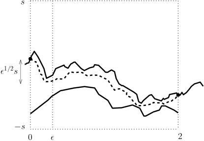
Refer to caption
Fig 2: Illustration for the proof of the 𝖥𝖺𝗅𝗅\mathsf{Fall} event. The top and bottom solid black curves are 𝔥t(1)​(⋅)\mathfrak{h}^{(1)}_{t}(\cdot) and 𝔥t(2)​(⋅)\mathfrak{h}^{(2)}_{t}(\cdot) respectively. The event that 𝔥t(1)​(y)−𝔥t(1)​(0)\mathfrak{h}^{(1)}_{t}(y)-\mathfrak{h}^{(1)}_{t}(0) is less than −ϵ1/2​s-\epsilon^{1/2}s for some y∈(0,ϵ)y\in(0,\epsilon) is 𝖥𝖺𝗅𝗅ϵ,s\mathsf{Fall}_{\epsilon,s}, and ℙ𝐇t1,2,(0,2),(𝔥t(1)​(0),𝔥t(1)​(2)),(+∞,𝔥t(2))​(𝖥𝖺𝗅𝗅ϵ,s)\mathbb{P}^{1,2,(0,2),(\mathfrak{h}^{(1)}_{t}(0),\mathfrak{h}^{(1)}_{t}(2)),(+\infty,\mathfrak{h}^{(2)}_{t})}_{\mathbf{H}_{t}}\big(\mathsf{Fall}_{\epsilon,s}\big) is the probability of 𝖥𝖺𝗅𝗅ϵ,s\mathsf{Fall}_{\epsilon,s} conditioned on the sigma algebra 𝔉ext​({1}×(0,2))\mathfrak{F}_{\mathrm{ext}}\big(\{1\}\times(0,2)\big) which is generated by everything outside of the first curve on the interval (0,2)(0,2). The dashed black curve is a free Brownian bridge B~\tilde{B} with law ℙfree(0,2),(𝔥t(1)​(0),𝔥t(2)​(2))\mathbb{P}^{(0,2),(\mathfrak{h}^{(1)}_{t}(0),\mathfrak{h}^{(2)}_{t}(2))}_{\mathrm{free}} coupled to 𝔥t(1)​(⋅)\mathfrak{h}^{(1)}_{t}(\cdot) so that it stays below 𝔥t(1)​(⋅)\mathfrak{h}^{(1)}_{t}(\cdot) on the interval (0,2)(0,2). Owing to this coupling, ℙ𝐇t1,2,(0,2),(𝔥t(1)​(0),𝔥t(1)​(2)),(+∞,𝔥t(2))​(𝖥𝖺𝗅𝗅ϵ,s)≤ℙfree(0,2),𝔥t(1)​(0),𝔥t(1)​(2)​(𝖥𝖺𝗅𝗅~ϵ,s)\mathbb{P}^{1,2,(0,2),(\mathfrak{h}^{(1)}_{t}(0),\mathfrak{h}^{(1)}_{t}(2)),(+\infty,\mathfrak{h}^{(2)}_{t})}_{\mathbf{H}_{t}}(\mathsf{Fall}_{\epsilon,s})\leq\mathbb{P}^{(0,2),\mathfrak{h}^{(1)}_{t}(0),\mathfrak{h}^{(1)}_{t}(2)}_{\mathrm{free}}(\widetilde{\mathsf{Fall}}_{\epsilon,s}) where 𝖥𝖺𝗅𝗅~ϵ,s\widetilde{\mathsf{Fall}}_{\epsilon,s} is the 𝖥𝖺𝗅𝗅\mathsf{Fall} event with B~\tilde{B} in place of 𝔥t(1)\mathfrak{h}^{(1)}_{t}. The probability of 𝖥𝖺𝗅𝗅~ϵ,s\widetilde{\mathsf{Fall}}_{\epsilon,s} under ℙfree(0,2),𝔥t(1)​(0),𝔥t(1)​(2)\mathbb{P}^{(0,2),\mathfrak{h}^{(1)}_{t}(0),\mathfrak{h}^{(1)}_{t}(2)}_{\mathrm{free}} conditioned on 𝔥t(1)​(0)≤s/4\mathfrak{h}^{(1)}_{t}(0)\leq s/4 and 𝔥t(1)(2)+2≥−s/4\mathfrak{h}^{(1)}_{t}(2)+2\geq-s/4 is maximized when 𝔥t(1)​(0)=s/4\mathfrak{h}^{(1)}_{t}(0)=s/4, and 𝔥t(1)(2)+2=−s/4\mathfrak{h}^{(1)}_{t}(2)+2=-s/4 and the maximum value is equal to the probability of infz∈[0,ϵ]​{B~​(z)+z2/2}\mathrm{inf}_{z\in[0,\epsilon]}\{\tilde{B}(z)+z^{2}/2\} being less than −s​ϵ1/2-s\epsilon^{1/2} where B~\tilde{B} is a Brownian bridge in [0,2][0,2] with B~​(0)=0\tilde{B}(0)=0 and B~​(2)=−2−2−1​s\tilde{B}(2)=-2-2^{-1}s. The reflection principle bounds this probability.

Recalling the notation from Definition 2.1, we will argue that

ℙ⁡(𝖥𝖺𝗅𝗅ϵ,s,𝖦ϵ,s)\displaystyle\mathbb{P}\Big(\mathsf{Fall}_{\epsilon,s},\mathsf{G}_{\epsilon,s}\Big) ≤ℙ(𝖥𝖺𝗅𝗅ϵ,s,𝔥t(1)(0)≤s/4,𝔥t(1)(2)+2≥−s/4)\displaystyle\leq\mathbb{P}\Big(\mathsf{Fall}_{\epsilon,s}\,,\,\mathfrak{h}^{(1)}_{t}(0)\leq s/4\,,\,\mathfrak{h}^{(1)}_{t}(2)+2\geq-s/4\,\Big) (77)
=𝔼[𝟏𝔥t(1)​(0)≤s/4⋅𝟏𝔥(1)t(2)+2≥−s/4⋅ℙ𝐇t1,1,(0,2),(𝔥t(1)​(0),𝔥t(1)​(2)),(+∞,𝔥t(2))(𝖥𝖺𝗅𝗅ϵ,s)]\displaystyle=\mathbb{E}\Big[\mathbf{1}_{\mathfrak{h}^{(1)}_{t}(0)\leq s/4}\cdot\mathbf{1}_{\mathfrak{h}^{(1)}_{t}(2)+2\geq-s/4}\cdot\mathbb{P}^{1,1,(0,2),(\mathfrak{h}^{(1)}_{t}(0),\mathfrak{h}^{(1)}_{t}(2)),(+\infty,\mathfrak{h}^{(2)}_{t})}_{\mathbf{H}_{t}}\big(\mathsf{Fall}_{\epsilon,s}\big)\Big] (78)
≤𝔼[𝟏𝔥t(1)​(0)≤s/4⋅𝟏𝔥(1)t(2)+2≥−s/4⋅ℙfree(0,2),𝔥t(1)​(0),𝔥t(1)​(2)(𝖥𝖺𝗅𝗅~ϵ,s)]\displaystyle\leq\mathbb{E}\Big[\mathbf{1}_{\mathfrak{h}^{(1)}_{t}(0)\leq s/4}\cdot\mathbf{1}_{\mathfrak{h}^{(1)}_{t}(2)+2\geq-s/4}\cdot\mathbb{P}^{(0,2),\mathfrak{h}^{(1)}_{t}(0),\mathfrak{h}^{(1)}_{t}(2)}_{\mathrm{free}}\big(\widetilde{\mathsf{Fall}}_{\epsilon,s}\big)\Big] (79)
≤sup{ℙfree(0,2),y,z(𝖥𝖺𝗅𝗅~ϵ,s):y≤s/4,z+2≥−s/4}\displaystyle\leq\sup\Big\{\mathbb{P}^{(0,2),y,z}_{\mathrm{free}}\big(\widetilde{\mathsf{Fall}}_{\epsilon,s}\big):y\leq s/4,z+2\geq-s/4\big\} (80)
=ℙfree(0,2),s/4,−2−4−1​s​(𝖥𝖺𝗅𝗅~ϵ,s),\displaystyle=\mathbb{P}^{(0,2),s/4,-2-4^{-1}s}_{\mathrm{free}}\big(\widetilde{\mathsf{Fall}}_{\epsilon,s}\big)\,, (81)

where we allow 𝖥𝖺𝗅𝗅~ϵ,s\widetilde{\mathsf{Fall}}_{\epsilon,s} to denote the 𝖥𝖺𝗅𝗅\mathsf{Fall} event with respect to the concerned Brownian bridge law. Here, the first line follows by dropping two of the conditions in 𝖦ϵ,s\mathsf{G}_{\epsilon,s}. The equality with the second line uses the Brownian Gibbs property for the KPZ line ensemble and conditional expectations with respect to the σ\sigma-field external to 𝔥t(1)\mathfrak{h}^{(1)}_{t} on the interval [0,2][0,2]. The inequality with the third line uses the monotone coupling (Lemma 2.4) to remove the second curve in the conditioning. Under this coupling, the curve 𝔥t(1)\mathfrak{h}^{(1)}_{t} is bounded below by a Brownian bridge B~\tilde{B} connecting the same endpoints. The inequality follows since the probability of the event 𝖥𝖺𝗅𝗅\mathsf{Fall} may only increase in response to the lowering of the curve. The inequality with the fourth line comes from maximizing over all values of 𝔥t(1)​(0)\mathfrak{h}^{(1)}_{t}(0) and 𝔥t(1)​(2)\mathfrak{h}^{(1)}_{t}(2) that satisfy the pair of conditions in the indicator functions of the preceding line. This maximum is achieved when the boundaries are maximally displaced; thus, the final equality.

We may rewrite the final term in (77) as ℙfree(0,2),s/4,−2−s/4​(𝖥𝖺𝗅𝗅~ϵ,s)=ℙ⁡(infz∈[0,ϵ]{B′​(z)+z22}≤−s​ϵ1/2)\mathbb{P}^{(0,2),s/4,-2-s/4}_{\mathrm{free}}\big(\widetilde{\mathsf{Fall}}_{\epsilon,s}\big)=\mathbb{P}\Big(\inf\limits_{z\in[0,\epsilon]}\big\{B^{\prime}(z)+\tfrac{z^{2}}{2}\big\}\leq-s\epsilon^{1/2}\Big) where B′:[0,2]→ℝB^{\prime}:[0,2]\to\mathbb{R} is a Brownian bridge with B′​(0)=0B^{\prime}(0)=0 and B′​(2)=−2−s2B^{\prime}(2)=-2-\tfrac{s}{2}; here, we shifted the whole system down by s/4s/4 to relocate the starting value to zero. Removing the parabola from the infimum only increases the probability. Now set B⁡(z)=B′​(z)−z2​(−2−s2)B(z)=B^{\prime}(z)-\tfrac{z}{2}(-2-\tfrac{s}{2}), so that BB is a Brownian bridge with B⁡(0)=B⁡(2)=0B(0)=B(2)=0. Taking into account the maximal effect of this linear shift shows that

ℙ⁡(infz∈[0,ϵ](B′​(z)+z22)≤−s​ϵ1/2)\displaystyle\mathbb{P}\Big(\!\inf_{z\in[0,\epsilon]}\!\big(B^{\prime}(z)+\tfrac{z^{2}}{2}\Big)\leq-s\epsilon^{1/2}\big) ≤ℙ⁡(infz∈[0,ϵ]B⁡(z)≤−s​ϵ1/2+ϵ2​(−2−s2))\displaystyle\leq\mathbb{P}\Big(\!\inf_{z\in[0,\epsilon]}\!B(z)\leq-s\epsilon^{1/2}+\tfrac{\epsilon}{2}(-2-\tfrac{s}{2})\Big)
≤ℙ⁡(infz∈[0,ϵ]B⁡(z)≤−s2​ϵ1/2).\displaystyle\leq\mathbb{P}\big(\!\inf_{z\in[0,\epsilon]}\!B(z)\leq-\tfrac{s}{2}\epsilon^{1/2}\big).

The latter inequality is due to ϵ2​(2+s2)≤s​ϵ1/2/2\tfrac{\epsilon}{2}(2+\tfrac{s}{2})\leq s\epsilon^{1/2}/2, a bound that holds for s≥4s\geq 4 – assuming ϵ∈(0,1]\epsilon\in(0,1], as we do. The right-hand probability can be estimated via the reflection principle, which yields the desired bound of the form c1​exp⁡(−c2​s2)c_{1}\exp(-c_{2}s^{2}) for suitable constants c1,c2>0c_{1},c_{2}>0.

Refer to caption
Fig 3: Illustration for the proof concerning the 𝖱𝗂𝗌𝖾\mathsf{Rise} event. The solid black curve is 𝔥t(1)​(⋅)\mathfrak{h}^{(1)}_{t}(\cdot). We start by rewriting the event 𝖱𝗂𝗌𝖾ϵ,s\mathsf{Rise}_{\epsilon,s} as {χ≤ϵ}\big\{\chi\leq\epsilon\big\} where χ\chi is the smallest x∈(0,ϵ]x\in(0,\epsilon] such that 𝔥t(1)​(x)−𝔥t(1)​(0)≥ϵ1/2​s\mathfrak{h}^{(1)}_{t}(x)-\mathfrak{h}^{(1)}_{t}(0)\geq\epsilon^{1/2}s; if no such xx satisfies this inequality, then χ=+∞\chi=+\infty. On the event χ≤ϵ\chi\leq\epsilon, the interval (χ,2)(\chi,2) forms a stopping domain, thus by the strong Gibbs property the law of 𝔥t(1)​(⋅)\mathfrak{h}^{(1)}_{t}(\cdot) on (χ,2)(\chi,2) is that of a Brownian bridge conditioned to stay above 𝔥t(2)\mathfrak{h}^{(2)}_{t} on that interval. We may couple 𝔥t(1)​(⋅)\mathfrak{h}^{(1)}_{t}(\cdot) to lie above a free Brownian bridge. At any time in (χ,2)(\chi,2), a Brownian bridge has probability one-half of being above the linear interpolation between its endpoints (see the diagonal line in the figure). On the event 𝖦ϵ,s\mathsf{G}_{\epsilon,s}, we can control the slope of such a linear interpolation by a constant cc time ss. Thus, between χ\chi and ϵ\epsilon, the linear interpolation may have dropped at most c​s​ϵcs\epsilon which, for ϵ\epsilon small enough is bounded by ϵ1/2​s/2\epsilon^{1/2}s/2. The means that, on the event that χ≤ϵ\chi\leq\epsilon, there is at least a one-half chance of 𝔥t(1)​(ϵ)−𝔥t(1)​(0)≥ϵ1/2​s/2\mathfrak{h}^{(1)}_{t}(\epsilon)-\mathfrak{h}^{(1)}_{t}(0)\geq\epsilon^{1/2}s/2. However, viewed with a backwards’ glance from position ϵ\epsilon, this occurrence is a 𝖥𝖺𝗅𝗅\mathsf{Fall} event; so that the just given argument concerning 𝖥𝖺𝗅𝗅\mathsf{Fall} yields a Gaussian tail for the probability of the event in question.

We now turn to prove the 𝖱𝗂𝗌𝖾\mathsf{Rise} bound in (76) (see also Figure 3 and its caption). Define χ\chi to be the infimum of x∈(0,ϵ]x\in(0,\epsilon] such that 𝔥t(1)​(x)−𝔥t(1)​(0)≥s​ϵ1/2\mathfrak{h}^{(1)}_{t}(x)-\mathfrak{h}^{(1)}_{t}(0)\geq s\epsilon^{1/2}; if no such points exist, χ\chi is set equal to +∞+\infty. Since

ℙ⁡(𝖱𝗂𝗌𝖾ϵ,s,𝖦ϵ,s)=ℙ⁡(χ≤ϵ,𝖦ϵ,s),\mathbb{P}(\mathsf{Rise}_{\epsilon,s},\mathsf{G}_{\epsilon,s})=\mathbb{P}(\chi\leq\epsilon,\mathsf{G}_{\epsilon,s}),

it suffices to bound the probability on the right-hand side, which we write in the form

ℙ(χ≤ϵ,𝖦ϵ,s,𝔥t(1)(χ)−𝔥t(1)(ϵ)<sϵ1/2/2)+ℙ(χ≤ϵ,𝖦ϵ,s,𝔥t(1)(χ)−𝔥t(1)(ϵ)≥sϵ1/2/2).\mathbb{P}\Big(\chi\leq\epsilon,\mathsf{G}_{\epsilon,s},\mathfrak{h}^{(1)}_{t}(\chi)-\mathfrak{h}^{(1)}_{t}(\epsilon)<s\epsilon^{1/2}/2\Big)\,+\,\mathbb{P}\Big(\chi\leq\epsilon,\mathsf{G}_{\epsilon,s},\mathfrak{h}^{(1)}_{t}(\chi)-\mathfrak{h}^{(1)}_{t}(\epsilon)\geq s\epsilon^{1/2}/2\Big)\,.

In the first displayed term, the occurrence of {χ≤ϵ}∩{𝔥t(1)(χ)−𝔥t(1)(ϵ)<sϵ1/2/2}\big\{\chi\leq\epsilon\big\}\cap\big\{\mathfrak{h}^{(1)}_{t}(\chi)-\mathfrak{h}^{(1)}_{t}(\epsilon)<s\epsilon^{1/2}/2\big\} entails that {𝔥t(1)(ϵ)−𝔥t(1)(0)≥sϵ1/2/2}\big\{\mathfrak{h}^{(1)}_{t}(\epsilon)-\mathfrak{h}^{(1)}_{t}(0)\geq s\epsilon^{1/2}/2\big\} holds, where note that continuity of 𝔥t(1)​(⋅)\mathfrak{h}^{(1)}_{t}(\cdot) implies that 𝔥t(1)​(χ)\mathfrak{h}^{(1)}_{t}(\chi) equals 𝔥t(1)​(0)+s​ϵ1/2\mathfrak{h}^{(1)}_{t}(0)+s\epsilon^{1/2}. By the argument concerning the 𝖥𝖺𝗅𝗅\mathsf{Fall} event, we can bound the probability of this occurrence by c1​exp⁡(−c2​s2)c_{1}\exp(-c_{2}s^{2}) for suitable constants c1c_{1} and c2c_{2}; this is why 𝖦ϵ,s\mathsf{G}_{\epsilon,s} involves control on 𝔥t(1)​(−2+ϵ)\mathfrak{h}^{(1)}_{t}(-2+\epsilon) and 𝔥t(1)​(ϵ)\mathfrak{h}^{(1)}_{t}(\epsilon). Since (χ,2)(\chi,2) is a strong stopping domain, by the strong Gibbs property (Lemma 2.2), we deduce the first bound in the next display, in whose second line, BB is ℙ𝐇t1,1,(χ,2),(𝔥t(1)​(χ),𝔥t(1)​(2)),(+∞,𝔥t(2))\mathbb{P}^{1,1,(\chi,2),(\mathfrak{h}^{(1)}_{t}(\chi),\mathfrak{h}^{(1)}_{t}(2)),(+\infty,\mathfrak{h}^{(2)}_{t})}_{\mathbf{H}_{t}}-distributed; in whose third line, BB is ℙfree(χ,2),𝔥t(1)​(χ),𝔥t(1)​(2)\mathbb{P}^{(\chi,2),\mathfrak{h}^{(1)}_{t}(\chi),\mathfrak{h}^{(1)}_{t}(2)}_{\mathrm{free}}-distributed; and in whose fourth line, B¯\bar{B} is the linear interpolation between (χ,B⁡(χ))\big(\chi,B(\chi)\big) and (2,B⁡(2))\big(2,B(2)\big).

ℙ(χ≤ϵ,𝖦ϵ,s,𝔥t(1)(χ)−𝔥t(1)(ϵ)≥sϵ1/2/2)\displaystyle\mathbb{P}\big(\chi\leq\epsilon,\mathsf{G}_{\epsilon,s},\mathfrak{h}^{(1)}_{t}(\chi)-\mathfrak{h}^{(1)}_{t}(\epsilon)\geq s\epsilon^{1/2}/2\big)
=\displaystyle= 𝔼⁡[𝟏χ≤ϵ,𝖦ϵ,s​ℙ𝐇t1,1,(χ,2),(𝔥t(1)​(χ),𝔥t(1)​(2)),(+∞,𝔥t(2))​(B⁡(χ)−B⁡(ϵ)≥s​ϵ1/2/2)]\displaystyle\mathbb{E}\Big[\mathbf{1}_{\chi\leq\epsilon,\mathsf{G}_{\epsilon,s}}\mathbb{P}^{1,1,(\chi,2),(\mathfrak{h}^{(1)}_{t}(\chi),\mathfrak{h}^{(1)}_{t}(2)),(+\infty,\mathfrak{h}^{(2)}_{t})}_{\mathbf{H}_{t}}\big(B(\chi)-B(\epsilon)\geq s\epsilon^{1/2}/2\big)\Big]
≤\displaystyle\leq 𝔼⁡[𝟏χ≤ϵ,𝖦ϵ,s​ℙfree(χ,2),𝔥t(1)​(χ),𝔥t(1)​(2)​(B⁡(χ)−B⁡(ϵ)≥s​ϵ1/2/2)]\displaystyle\mathbb{E}\Big[\mathbf{1}_{\chi\leq\epsilon,\mathsf{G}_{\epsilon,s}}\mathbb{P}^{(\chi,2),\mathfrak{h}^{(1)}_{t}(\chi),\mathfrak{h}^{(1)}_{t}(2)}_{\mathrm{free}}\big(B(\chi)-B(\epsilon)\geq s\epsilon^{1/2}/2\big)\Big]
≤\displaystyle\leq 𝔼⁡[𝟏χ≤ϵ,𝖦ϵ,s​ℙfree(χ,2),𝔥t(1)​(χ),𝔥t(1)​(2)​(B⁡(ϵ)≤B¯​(ϵ))]\displaystyle\mathbb{E}\Big[\mathbf{1}_{\chi\leq\epsilon,\mathsf{G}_{\epsilon,s}}\mathbb{P}^{(\chi,2),\mathfrak{h}^{(1)}_{t}(\chi),\mathfrak{h}^{(1)}_{t}(2)}_{\mathrm{free}}\big(B(\epsilon)\leq\bar{B}(\epsilon)\big)\Big]
=\displaystyle= 12​𝔼​[𝟏χ≤ϵ,𝖦ϵ,s].\displaystyle\tfrac{1}{2}\,\mathbb{E}\Big[\mathbf{1}_{\chi\leq\epsilon,\mathsf{G}_{\epsilon,s}}\Big]\,.

The inequality between the second and third line comes from applying the monotone coupling (Lemma 2.4). To justify the inequality between the third and fourth lines takes a bit more work. We claim that, on the event {χ≤ϵ,𝖦ϵ,s}\big\{\chi\leq\epsilon,\mathsf{G}_{\epsilon,s}\big\}, and as long as ϵ\epsilon is small enough, the condition B⁡(χ)−B⁡(ϵ)≥s​ϵ1/2/2B(\chi)-B(\epsilon)\geq s\epsilon^{1/2}/2 entails that B​(ϵ)≤B¯​(ϵ)B(\epsilon)\leq\bar{B}(\epsilon). This is because the maximal slope of B¯\bar{B} is a constant multiple cc of ss, and the maximal displacement of ϵ−χ\epsilon-\chi is ϵ\epsilon. Thus B¯​(ϵ)≥B⁡(χ)−c​s​ϵ\bar{B}(\epsilon)\geq B(\chi)-cs\epsilon. For ϵ\epsilon small enough, c​s​ϵ≤s​ϵ1/2/2cs\epsilon\leq s\epsilon^{1/2}/2; thus, B¯​(ϵ)≥B⁡(χ)−s​ϵ1/2/2\bar{B}(\epsilon)\geq B(\chi)-s\epsilon^{1/2}/2. This can be rewritten as B¯​(ϵ)+s​ϵ1/2/2≥B⁡(χ)\bar{B}(\epsilon)+s\epsilon^{1/2}/2\geq B(\chi), and B⁡(χ)−B⁡(ϵ)≥s​ϵ1/2/2B(\chi)-B(\epsilon)\geq s\epsilon^{1/2}/2 can be rewritten as B⁡(χ)≥B⁡(ϵ)+s​ϵ1/2/2B(\chi)\geq B(\epsilon)+s\epsilon^{1/2}/2. Combining these two yields B¯​(ϵ)≥B​(ϵ)\bar{B}(\epsilon)\geq B(\epsilon), as claimed. The final equality is simply from Brownian bridge having probability one-half of being below its linear interpolation at any given time.

Putting this all together, we have proved that

ℙ⁡(χ≤ϵ,𝖦ϵ,s)≤c1​exp⁡(−c2​s2)+12​ℙ​(χ≤ϵ,𝖦ϵ,s),\mathbb{P}\big(\chi\leq\epsilon,\mathsf{G}_{\epsilon,s}\big)\leq c_{1}\exp(-c_{2}s^{2})+\tfrac{1}{2}\mathbb{P}\big(\chi\leq\epsilon,\mathsf{G}_{\epsilon,s}\big),

which implies that

ℙ⁡(χ≤ϵ,𝖦ϵ,s)≤2​c1​exp⁡(−c2​s2),\mathbb{P}\big(\chi\leq\epsilon,\mathsf{G}_{\epsilon,s}\big)\leq 2c_{1}\exp(-c_{2}s^{2}),

as desired to prove the 𝖱𝗂𝗌𝖾\mathsf{Rise} bound in (76). ∎

Applying Propositions 4.1 and 4.2, there exist s0=s0​(t0)s_{0}=s_{0}(t_{0}) and c=c⁡(t0)c=c(t_{0}) such that, for x∈ℝx\in\mathbb{R}, t≥t0t\geq t_{0} and s≥s0s\geq s_{0}, ℙ⁡(¬𝖦ϵ,s​(x))≤exp⁡(−c​s3/2)\mathbb{P}\big(\neg\mathsf{G}_{\epsilon,s}(x)\big)\leq\exp\big(-cs^{3/2}\big). This inference and Proposition 4.3 yield (7); thus is the theorem proved. ∎

We will need one more result, concerning tails of increments.

Proposition 4.4.

For any t0>0t_{0}>0, ν>0\nu>0 and ϵ∈(0,1)\epsilon\in(0,1), there exist s=s⁡(t0,ν,ϵ)s=s(t_{0},\nu,\epsilon) and c=c⁡(t0,ν,ϵ)c=c(t_{0},\nu,\epsilon) such that, for t≥t0t\geq t_{0}, s≥s0s\geq s_{0} and θ>1\theta>1,

ℙ(supx∈[0,θ1/3]{𝔥t(θ−2/3x)−𝔥t(0)−θ−1/3ν​x22}≥θ−1/3s)≤exp(−cs9​(1−ϵ)/8),\displaystyle\mathbb{P}\Big(\sup_{x\in[0,\theta^{1/3}]}\big\{\mathfrak{h}_{t}(\theta^{-2/3}x)-\mathfrak{h}_{t}(0)-\theta^{-1/3}\tfrac{\nu x^{2}}{2}\big\}\geq\theta^{-1/3}s\Big)\leq\exp(-cs^{9(1-\epsilon)/8})\,, (82)
ℙ(infx∈[0,θ1/3]{𝔥t(θ−2/3x)−𝔥t(0)+θ−1/3ν​x22}≤−θ−1/3s)≤exp(−cs9​(1−ϵ)/8).\displaystyle\mathbb{P}\Big(\inf_{x\in[0,\theta^{1/3}]}\big\{\mathfrak{h}_{t}(\theta^{-2/3}x)-\mathfrak{h}_{t}(0)+\theta^{-1/3}\tfrac{\nu x^{2}}{2}\big\}\leq-\theta^{-1/3}s\Big)\leq\exp(-cs^{9(1-\epsilon)/8})\,. (83)

We prove only (82), since a very similar argument yields (83). Let 𝖤\mathsf{E} denote the event on the left-hand side of (82). Suppose first that θ<23\theta<2^{3}. Then

ℙ⁡(𝖤)≤ℙ⁡(supx∈[0,2]{𝔥t​(x)−𝔥t​(0)}≥s2)≤ℙ⁡(supx∈ℝ𝔥t​(x)≥s4)+ℙ⁡(𝔥t​(0)≤−s4).\displaystyle\mathbb{P}\big(\mathsf{E}\big)\leq\mathbb{P}\Big(\sup_{x\in[0,2]}\big\{\mathfrak{h}_{t}(x)-\mathfrak{h}_{t}(0)\big\}\geq\frac{s}{2}\Big)\leq\mathbb{P}\Big(\sup_{x\in\mathbb{R}}\mathfrak{h}_{t}(x)\geq\frac{s}{4}\Big)+\mathbb{P}\Big(\mathfrak{h}_{t}(0)\leq-\frac{s}{4}\Big)\,. (84)

The first bound is due to the supremum increasing in response to the omission of the parabola and extension of the range of xx to [0,2][0,2]. The second bound uses supx∈[0,21/3]𝔥t​(x)≤supx∈ℝ𝔥t​(x)\sup_{x\in[0,2^{1/3}]}\mathfrak{h}_{t}(x)\leq\sup_{x\in\mathbb{R}}\mathfrak{h}_{t}(x) and

{supx∈[0,2]{𝔥t(x)−𝔥t(0)}≥s/2}⊂{supx∈ℝ𝔥t(x)≥s/4}∪{𝔥t(0)≤−s/4}.\displaystyle\Big\{\sup_{x\in[0,2]}\big\{\mathfrak{h}_{t}(x)-\mathfrak{h}_{t}(0)\big\}\geq s/2\Big\}\subset\Big\{\sup_{x\in\mathbb{R}}\mathfrak{h}_{t}(x)\geq s/4\Big\}\cup\Big\{\mathfrak{h}_{t}(0)\leq-s/4\Big\}\,. (85)

Propositions 2.11 and 4.2 provide bounds on the right-hand probabilities in (84) of the form exp⁡(−c​s3/2)\exp(-cs^{3/2}), for some c=c⁡(t0)>0c=c(t_{0})>0 when s>s0​(t0)s>s_{0}(t_{0}) is large enough. This proves (82) for θ<23\theta<2^{3}.

Now suppose that θ≥23\theta\geq 2^{3}. We may partition [1,θ1/3]=⨆ℓ=13​K0+1ℐℓ[1,\theta^{1/3}]=\bigsqcup_{\ell=1}^{3K_{0}+1}\mathcal{I}_{\ell} where K0:=⌊13​log2​θ⌋K_{0}:=\lfloor\frac{1}{3}\log_{2}\theta\rfloor and ℐℓ:=[2(ℓ−1)/3,2ℓ/3]\mathcal{I}_{\ell}:=[2^{(\ell-1)/3},2^{\ell/3}] for 1≤ℓ≤3​K01\leq\ell\leq 3K_{0} and ℐ3​K0+1:=[2K0,θ1/3]\mathcal{I}_{3K_{0}+1}:=[2^{K_{0}},\theta^{1/3}]. For 1≤ℓ≤3​K0+11\leq\ell\leq 3K_{0}+1, define

𝒬ℓ:={supx∈ℐℓ{𝔥t(θ−2/3x)−𝔥t(0)}≥θ−1/3(s+ν​22​(ℓ−1)/32)}.\displaystyle\mathcal{Q}_{\ell}:=\bigg\{\sup_{x\in\mathcal{I}_{\ell}}\big\{\mathfrak{h}_{t}(\theta^{-2/3}x)-\mathfrak{h}_{t}(0)\big\}\geq\theta^{-1/3}\Big(s+\frac{\nu 2^{2(\ell-1)/3}}{2}\Big)\bigg\}\,. (86)

We seek to apply Proposition 4.3. This proposition will bound ℙ⁡(𝒬ℓ∩𝖦ℓ)\mathbb{P}(\mathcal{Q}_{\ell}\cap\mathsf{G}_{\ell}) for an event 𝖦ℓ\mathsf{G}_{\ell} that we will define soon. Before doing that, let us observe that if, in the 𝒬ℓ\mathcal{Q}_{\ell} event, we replace x∈ℐℓx\in\mathcal{I}_{\ell} by x∈[0,2ℓ/3]x\in[0,2^{\ell/3}], then the probability may only rise. Similarly, if we replace θ−1/3(s+ν​22​(ℓ−1)/32)\theta^{-1/3}\Big(s+\frac{\nu 2^{2(\ell-1)/3}}{2}\Big) by a smaller number, then the probability may also only rise. In realizing this second action, we will use the weighted arithmetic-geometric mean inequality to bound (see below for notational choices)

s+ν​22​(ℓ−1)/32=w1⋅sw1+w2⋅ν2​w2​22​(ℓ−1)/3\displaystyle s+\frac{\nu 2^{2(\ell-1)/3}}{2}=w_{1}\cdot\frac{s}{w_{1}}+w_{2}\cdot\frac{\nu}{2w_{2}}2^{2(\ell-1)/3} ≥22​w2​(ℓ−1)/3​(ν2​w2)w2​(sw1)w1\displaystyle\geq 2^{2w_{2}(\ell-1)/3}\Big(\frac{\nu}{2w_{2}}\Big)^{w_{2}}\Big(\frac{s}{w_{1}}\Big)^{w_{1}} (87)
≥aℓ(1+3​ϵ)/4​(s3)(3/4)​(1−ϵ)\displaystyle\geq a_{\ell}^{(1+3\epsilon)/4}\Big(\frac{s}{3}\Big)^{(3/4)(1-\epsilon)} (88)

where ϵ∈(0,1)\epsilon\in(0,1) is arbitrary, w1=3​(1−ϵ)4w_{1}=\tfrac{3(1-\epsilon)}{4}, w2=(1+3​ϵ)4w_{2}=\tfrac{(1+3\epsilon)}{4} and aℓ=ν2​(1+3​ϵ)​22​(ℓ−1)/3a_{\ell}=\frac{\nu}{2(1+3\epsilon)}2^{2(\ell-1)/3}. The last inequality of the above display follows by substituting aℓa_{\ell} and noting that s/w1≥s/3s/w_{1}\geq s/3. This means that

ℙ⁡(𝒬ℓ∩𝖦ℓ)\displaystyle\mathbb{P}(\mathcal{Q}_{\ell}\cap\mathsf{G}_{\ell}) ≤ℙ({supx∈[0,2ℓ/3]{𝔥t(θ−2/3x)−𝔥t(0)}≥θ−1/3aℓ(1+3​ϵ)/4(s/3)(3/4)​(1−ϵ)}∩𝖦ℓ)\displaystyle\leq\mathbb{P}\Big(\Big\{\sup_{x\in[0,2^{\ell/3}]}\big\{\mathfrak{h}_{t}(\theta^{-2/3}x)-\mathfrak{h}_{t}(0)\big\}\geq\theta^{-1/3}a^{(1+3\epsilon)/4}_{\ell}(s/3)^{(3/4)(1-\epsilon)}\Big\}\cap\mathsf{G}_{\ell}\Big) (89)
=ℙ({supx∈[0,ϵℓ]{𝔥t(x)−𝔥t(0)}≥sℓϵℓ1/2}∩𝖦ℓ),\displaystyle=\mathbb{P}\Big(\Big\{\sup_{x\in[0,\epsilon_{\ell}]}\big\{\mathfrak{h}_{t}(x)-\mathfrak{h}_{t}(0)\big\}\geq s_{\ell}\epsilon_{\ell}^{1/2}\Big\}\cap\mathsf{G}_{\ell}\Big), (90)

where in the second line we have used the notation ϵℓ=2ℓ/3θ−2/3\epsilon_{\ell}=2^{\ell/3}\theta^{-2/3} and

sℓ=2ϵ​ℓ−(1+3​ϵ)6​(ν2​(1+3​ϵ))(1+3​ϵ)/4​(s3)(3/4)​(1−ϵ),s_{\ell}=2^{\tfrac{\epsilon\ell-(1+3\epsilon)}{6}}\Big(\frac{\nu}{2(1+3\epsilon)}\Big)^{(1+3\epsilon)/4}\Big(\frac{s}{3}\Big)^{(3/4)(1-\epsilon)},

and performed a simple change over variables.

By the definition of 𝒬ℓ\mathcal{Q}_{\ell}, 𝖤⊂⋃ℓ=13​K0+1𝒬ℓ\mathsf{E}\subset\bigcup^{3K_{0}+1}_{\ell=1}\mathcal{Q}_{\ell}. Choosing 𝖦ℓ=𝖦ϵℓ,sℓ\mathsf{G}_{\ell}=\mathsf{G}_{\epsilon_{\ell},s_{\ell}} from (74), by the union bound,

ℙ⁡(𝖤)≤∑ℓ=13​K0+1(ℙ⁡(𝒬ℓ∩𝖦ℓ)+ℙ⁡(¬𝖦ℓ)).\displaystyle\mathbb{P}\big(\mathsf{E}\big)\leq\sum_{\ell=1}^{3K_{0}+1}\Big(\mathbb{P}(\mathcal{Q}_{\ell}\cap\mathsf{G}_{\ell})+\mathbb{P}(\neg\mathsf{G}_{\ell})\Big)\,. (91)

Propositions 2.11 and 2.12 furnish s0=s0​(t0,ν,ϵ)s_{0}=s_{0}(t_{0},\nu,\epsilon) and c=c⁡(t0,ν,ϵ)c=c(t_{0},\nu,\epsilon) such that, for ℓ≥1\ell\geq 1 and s>s0s>s_{0},

ℙ⁡(¬𝖦ℓ)≤exp⁡(−c​sℓ3/2)=exp⁡(−c​2ϵ⁡(ℓ−3)/4​s98​(1−ϵ)).\displaystyle\mathbb{P}(\neg\mathsf{G}_{\ell})\leq\exp\big(-cs_{\ell}^{3/2}\big)=\exp\big(-c2^{\epsilon(\ell-3)/4}s^{\frac{9}{8}(1-\epsilon)}\big). (92)

The sum over ℓ\ell of such a bound produces an upper bound of the desired form exp⁡(−c​s9​(1−ϵ)/8)\exp(-cs^{9(1-\epsilon)/8}). Turning to ℙ⁡(𝒬ℓ∩𝖦ℓ)\mathbb{P}\big(\mathcal{Q}_{\ell}\cap\mathsf{G}_{\ell}\big), we may apply Proposition 4.3 with ϵ=ϵℓ\epsilon=\epsilon_{\ell} and s=sℓs=s_{\ell}. The result is precisely the same sort of bound as on ℙ⁡(¬𝖦ℓ)\mathbb{P}(\neg\mathsf{G}_{\ell}) above; hence, by summing over ℓ\ell, we again recover the sought upper bound, of the form exp⁡(−c​s9​(1−ϵ)/8)\exp(-cs^{9(1-\epsilon)/8}). This completes the proof of (82). ∎

5 Remote correlation: Proof of Theorem 1.1

The composition law from Proposition 2.9 will figure prominently in this argument since it permits us to describe the two-time distribution in terms of spatial processes that we understand well. Recall that this result shows that, for α>1\alpha>1 given, we may write 𝔥t​(α,0)\mathfrak{h}_{t}(\alpha,0) as the composition of independent spatial processes 𝔥t​(1,⋅)\mathfrak{h}_{t}(1,\cdot) and 𝔥α​t↓t​(⋅)\mathfrak{h}_{\alpha t\downarrow t}(\cdot). The latter is distributed as 𝔥t​(α−1,⋅)\mathfrak{h}_{t}(\alpha-1,\cdot). We will use a suggestive shorthand, in the spirit of 𝔥α​t↓t\mathfrak{h}_{\alpha t\downarrow t}:

𝔥0↑t​(⋅):=𝔥t​(1,⋅),𝔥0↑α​t​(⋅):=𝔥t​(α,⋅);\displaystyle\mathfrak{h}_{0\uparrow t}(\cdot):=\mathfrak{h}_{t}(1,\cdot),\qquad\mathfrak{h}_{0\uparrow\alpha t}(\cdot):=\mathfrak{h}_{t}(\alpha,\cdot)\,; (93)

and, when we write 𝔥0↑t\mathfrak{h}_{0\uparrow t}, we mean 𝔥0↑t​(0)\mathfrak{h}_{0\uparrow t}(0); and likewise for 𝔥0↑α​t\mathfrak{h}_{0\uparrow\alpha t} and 𝔥α​t↓t\mathfrak{h}_{\alpha t\downarrow t}. The shorthand is intended to suggest that the value of 𝔥0↑α​t​(0)\mathfrak{h}_{0\uparrow\alpha t}(0) from time zero to α​t\alpha t is obtained via the integral operation ItI_{t} by composing the function 𝔥0↑t​(⋅)\mathfrak{h}_{0\uparrow t}(\cdot) with 𝔥α​t↓t​(⋅)\mathfrak{h}_{\alpha t\downarrow t}(\cdot), the latter under the opposite direction of time. The shorthand will cause confusion if 𝔥0↑t\mathfrak{h}_{0\uparrow t} or 𝔥0↑α​t\mathfrak{h}_{0\uparrow\alpha t} are regarded as functions of tt or α\alpha. These two parameters are, however, given: the variable ‘⋅\cdot’ in (93) is spatial.

This section’s goal is to prove the bounds (4) in Theorem 1.1 which in our new notation are:

c1α−1/3≤Corr(𝔥0↑t,𝔥0↑α​t)≤c2α−1/3.\displaystyle c_{1}\alpha^{-1/3}\leq\mathrm{Corr}\Big(\mathfrak{h}_{0\uparrow t},\mathfrak{h}_{0\uparrow\alpha t}\Big)\leq c_{2}\alpha^{-1/3}\,. (94)

The derivation of Theorem 1.1 depends on two principal results, Propositions 5.1 and 5.2. We state these; use them to prove the theorem; and then prove them in turn.

Define 𝒜high={𝔥0↑α​t−𝔥α​t↓t−𝔥0↑t≥s}\mathcal{A}_{\mathrm{high}}=\big\{\mathfrak{h}_{0\uparrow\alpha t}-\mathfrak{h}_{\alpha t\downarrow t}-\mathfrak{h}_{0\uparrow t}\geq s\big\} and 𝒜low={𝔥0↑α​t−𝔥α​t↓t−𝔥0↑t≤−t−1/3s}\mathcal{A}_{\mathrm{low}}=\big\{\mathfrak{h}_{0\uparrow\alpha t}-\mathfrak{h}_{\alpha t\downarrow t}-\mathfrak{h}_{0\uparrow t}\leq-t^{-1/3}s\big\}.

Proposition 5.1.

For any t0>0t_{0}>0 and α0>1\alpha_{0}>1, there exist s0=s0​(t0,α0)>0s_{0}=s_{0}(t_{0},\alpha_{0})>0 and c=c⁡(t0,α0)>0c=c(t_{0},\alpha_{0})>0 such that, for s≥s0s\geq s_{0}, t>t0t>t_{0} and α>α0\alpha>\alpha_{0},

ℙ⁡(𝒜high)≤exp⁡(−c​s3/4).\displaystyle\mathbb{P}\big(\mathcal{A}_{\mathrm{high}}\big)\leq\exp(-cs^{3/4})\,. (95)
Proposition 5.2.

For any t0>0t_{0}>0, there exist s0=s0​(t0)>0s_{0}=s_{0}(t_{0})>0 and c=c⁡(t0)>0c=c(t_{0})>0 such that, for s≥s0s\geq s_{0}, t>t0t>t_{0} and α>2\alpha>2,

ℙ⁡(𝒜low)≤exp⁡(−c​s3/2).\displaystyle\mathbb{P}\big(\mathcal{A}_{\mathrm{low}}\big)\leq\exp\big(-cs^{3/2}\big)\,. (96)

Further, for any t0>0t_{0}>0, α0>1\alpha_{0}>1 and δ>0\delta>0, there exist s0=s0​(t0,α0,δ)>0s_{0}=s_{0}(t_{0},\alpha_{0},\delta)>0 and c=c⁡(t0,α0,δ)>0c=c(t_{0},\alpha_{0},\delta)>0 such that, for s≥s0s\geq s_{0}, t>t0t>t_{0} and α>α0\alpha>\alpha_{0},

ℙ⁡(𝒜low|𝔥0↑t≥𝔼⁡[𝔥0↑t]+δ)≤exp⁡(−c​s3/2).\displaystyle\mathbb{P}\,\Big(\mathcal{A}_{\mathrm{low}}\,\Big|\,\mathfrak{h}_{0\uparrow t}\geq\mathbb{E}\big[\mathfrak{h}_{0\uparrow t}\big]+\delta\Big)\,\leq\,\exp\big(-cs^{3/2}\big)\,. (97)

The two results address the rarity of the events that 𝔥0↑α​t\mathfrak{h}_{0\uparrow\alpha t} significantly exceeds, or falls below, 𝔥0↑t+𝔥α​t↓t\mathfrak{h}_{0\uparrow t}+\mathfrak{h}_{\alpha t\downarrow t}. Note that, in the latter case – via the definition of 𝒜low\mathcal{A}_{\mathrm{low}} – deviation is measured on scale t−1/3t^{-1/3}. To interpret the two results and the latter choice of scaling, it may be helpful to consider the composition law and the supremum variational problem obtained in the high tt limit which was a focus of attention in Section 3. In the high tt case, a counterpart to Proposition 5.1 would examine the tail of the difference between the variational problem’s solution and the value of the pair sum associated to the choice of location zero at the intermediate time. In this t↗∞t\nearrow\infty limit, Proposition 5.2 would become trivial, because the difference in question can never be negative. Back in our finite tt world, the softening of the variational problem leads to a degree of violation to this strict ordering. The t−1/3t^{-1/3} tail that we study probes the extent of this violation.

We first show the following stronger version of the upper bound on the correlation in (94): for any t0>0t_{0}>0, there exist c2=c2​(0)>0c_{2}=c_{2}(0)>0 such that, for t>t0t>t_{0}, and α>2\alpha>2, |Corr(𝔥0↑α​t,𝔥0↑t)|≤c2α−1/3|\mathrm{Corr}(\mathfrak{h}_{0\uparrow\alpha t},\mathfrak{h}_{0\uparrow t})|\leq c_{2}\alpha^{-1/3}. Recall that, by definition,

Corr⁡(𝔥0↑t,𝔥0↑α​t)=Cov⁡(𝔥0↑α​t,𝔥0↑t)Var⁡(𝔥0↑α​t)​Var⁡(𝔥0↑t).\displaystyle\mathrm{Corr}\big(\mathfrak{h}_{0\uparrow t},\mathfrak{h}_{0\uparrow\alpha t}\big)=\frac{\mathrm{Cov}\big(\mathfrak{h}_{0\uparrow\alpha t},\mathfrak{h}_{0\uparrow t}\big)}{\sqrt{\mathrm{Var}(\mathfrak{h}_{0\uparrow\alpha t})}\sqrt{\mathrm{Var}(\mathfrak{h}_{0\uparrow t})}}\,. (98)

Under the coupling provided by Proposition 2.9, 𝔥α​t↓t\mathfrak{h}_{\alpha t\downarrow t} and 𝔥0↑t\mathfrak{h}_{0\uparrow t} are independent. Hence,

|Cov\displaystyle\big|\mathrm{Cov} (𝔥0↑α​t,𝔥0↑t)|=Cov⁡(𝔥0↑α​t−𝔥α​t↓t−𝔥0↑t,𝔥0↑t)+Var⁡(𝔥0↑t).\displaystyle\big(\mathfrak{h}_{0\uparrow\alpha t},\mathfrak{h}_{0\uparrow t}\big)\big|=\mathrm{Cov}\big(\mathfrak{h}_{0\uparrow\alpha t}-\mathfrak{h}_{\alpha t\downarrow t}-\mathfrak{h}_{0\uparrow t},\mathfrak{h}_{0\uparrow t}\big)+\mathrm{Var}\big(\mathfrak{h}_{0\uparrow t}\big)\,. (99)

Applying the Cauchy-Schwarz inequality to the first term yields

|Cov(𝔥0↑α​t\displaystyle\big|\mathrm{Cov}\big(\mathfrak{h}_{0\uparrow\alpha t} OPEN−𝔥α​t↓t−𝔥0↑t,𝔥0↑t)|≤Var⁡(𝔥0↑α​t−𝔥α​t↓t−𝔥0↑t)​Var​(𝔥0↑t).\displaystyle-\mathfrak{h}_{\alpha t\downarrow t}-\mathfrak{h}_{0\uparrow t},\mathfrak{h}_{0\uparrow t}\big)\big|\leq\sqrt{\mathrm{Var}\big(\mathfrak{h}_{0\uparrow\alpha t}-\mathfrak{h}_{\alpha t\downarrow t}-\mathfrak{h}_{0\uparrow t}\big)\,\mathrm{Var}(\mathfrak{h}_{0\uparrow t})}\,. (100)

Substituting (99) into and applying (100) to (98) then leads to

|Corr\displaystyle\big|\mathrm{Corr} (𝔥0↑α​t,𝔥0↑t)|≤Var⁡(𝔥0↑α​t−𝔥α​t↓t−𝔥0↑t)Var⁡(𝔥0↑α​t)+Var⁡(𝔥0↑t)Var⁡(𝔥0↑α​t).\displaystyle(\mathfrak{h}_{0\uparrow\alpha t},\mathfrak{h}_{0\uparrow t})\big|\leq\frac{\sqrt{\mathrm{Var}(\mathfrak{h}_{0\uparrow\alpha t}-\mathfrak{h}_{\alpha t\downarrow t}-\mathfrak{h}_{0\uparrow t})}}{\sqrt{\mathrm{Var}(\mathfrak{h}_{0\uparrow\alpha t})}}+\frac{\sqrt{\mathrm{Var}(\mathfrak{h}_{0\uparrow t})}}{\sqrt{\mathrm{Var}(\mathfrak{h}_{0\uparrow\alpha t})}}\,. (101)

The tail bounds on 𝔥t​(0)\mathfrak{h}_{t}(0) (or on 𝔥0↑t\mathfrak{h}_{0\uparrow t}) from Propositions 2.11 and 2.12 imply via Lemma 8.4 that there exist c=c⁡(t0)>0c=c(t_{0})>0 and C=C⁡(t0)>0C=C(t_{0})>0 such that

c≤Var⁡(𝔥0↑t)≤C,andc​α2/3≤Var⁡(𝔥0↑α​t)≤C​α2/3.\displaystyle c\leq\mathrm{Var}\big(\mathfrak{h}_{0\uparrow t}\big)\leq C\,,\qquad\textrm{and}\quad c\alpha^{2/3}\leq\mathrm{Var}\big(\mathfrak{h}_{0\uparrow\alpha t}\big)\leq C\alpha^{2/3}\,. (102)

Here, the second bound uses 𝔥0→α​t=(d)𝔥α​t​(1,0)​α1/3\mathfrak{h}_{0\to\alpha t}\stackrel{{\scriptstyle(d)}}{{=}}\mathfrak{h}_{\alpha t}(1,0)\alpha^{1/3}. Similarly, Propositions  5.1 and  5.2 imply that

Var⁡(𝔥0↑α​t−𝔥α​t↓t−𝔥0↑t)≤C.\displaystyle\mathrm{Var}\big(\mathfrak{h}_{0\uparrow\alpha t}-\mathfrak{h}_{\alpha t\downarrow t}-\mathfrak{h}_{0\uparrow t}\big)\leq C\,. (103)

Substituting (102) and (103) into the right-hand side of (101) yields

|Corr(𝔥0↑α​t,𝔥0↑t)|≤c2α−1/3\displaystyle\big|\mathrm{Corr}(\mathfrak{h}_{0\uparrow\alpha t},\mathfrak{h}_{0\uparrow t})\big|\leq c_{2}\alpha^{-1/3} (104)

for a constant c2=c2​(t0)>0c_{2}=c_{2}(t_{0})>0. This is the strengthened upper bound that we have sought.

Now we turn to prove the lower bound in (94). Assume for now that t>1t>1, though we will eventually need to impose that t>t0t>t_{0} for t0t_{0} sufficiently large. The lower bound will arise from an appeal to Corollary 8.2 with X:=𝔥0↑α​tX:=\mathfrak{h}_{0\uparrow\alpha t} and Y:=𝔥0↑tY:=\mathfrak{h}_{0\uparrow t}. The other two parameters in the corollary, C1C_{1} and C2C_{2}, will be specified after the next calculation, which will inform our choice of their value. Observe that, for y:=𝔼⁡[𝔥0↑t]+δy:=\mathbb{E}[\mathfrak{h}_{0\uparrow t}]+\delta with δ>0\delta>0,

𝔼⁡[𝔥0↑α​t|𝔥0↑t≥y]≥𝔼⁡[𝔥α​t↓t]+y+𝔼⁡[𝔥0↑α​t−𝔥α​t↓t−𝔥0↑t|𝔥0↑t≥y].\mathbb{E}\Big[\mathfrak{h}_{0\uparrow\alpha t}\big|\mathfrak{h}_{0\uparrow t}\geq y\Big]\geq\mathbb{E}\big[\mathfrak{h}_{\alpha t\downarrow t}\big]+y+\mathbb{E}\Big[\mathfrak{h}_{0\uparrow\alpha t}-\mathfrak{h}_{\alpha t\downarrow t}-\mathfrak{h}_{0\uparrow t}\big|\mathfrak{h}_{0\uparrow t}\geq y\Big]\,.

This bound follows from 𝔼⁡[𝔥α​t↓t|𝔥0↑t≥y]=𝔼⁡[𝔥α​t↓t]\mathbb{E}\big[\mathfrak{h}_{\alpha t\downarrow t}|\mathfrak{h}_{0\uparrow t}\geq y\big]=\mathbb{E}[\mathfrak{h}_{\alpha t\downarrow t}] – a consequence of the independence of 𝔥0↑t\mathfrak{h}_{0\uparrow t} and 𝔥α​t↓t\mathfrak{h}_{\alpha t\downarrow t} – and the trivial 𝔼⁡[𝔥0↑t|𝔥0↑t≥y]≥y\mathbb{E}\big[\mathfrak{h}_{0\uparrow t}|\mathfrak{h}_{0\uparrow t}\geq y\big]\geq y. Next note that

𝔼[𝔥0↑α​t−𝔥α​t↓t−𝔥0↑t|𝔥0↑t≥y]≥𝔼[min{0,𝔥0↑α​t−𝔥α​t↓t−𝔥0↑t|𝔥0↑t≥y]\displaystyle\mathbb{E}\,\Big[\,\mathfrak{h}_{0\uparrow\alpha t}-\mathfrak{h}_{\alpha t\downarrow t}-\mathfrak{h}_{0\uparrow t}\,\Big|\,\mathfrak{h}_{0\uparrow t}\geq y\,\Big]\,\geq\,\mathbb{E}\,\Big[\,\min\{0,\mathfrak{h}_{0\uparrow\alpha t}-\mathfrak{h}_{\alpha t\downarrow t}-\mathfrak{h}_{0\uparrow t}\,\Big|\,\mathfrak{h}_{0\uparrow t}\geq y\,\Big] (105)
=\displaystyle= −t−1/3∫0∞ℙ(𝔥0↑α​t−𝔥α​t↓t−𝔥0↑t≤−t−1/3s|𝔥0↑t≥y)ds≥−t−1/3c(δ)\displaystyle-t^{-1/3}\int^{\infty}_{0}\mathbb{P}\Big(\mathfrak{h}_{0\uparrow\alpha t}-\mathfrak{h}_{\alpha t\downarrow t}-\mathfrak{h}_{0\uparrow t}\leq-t^{-1/3}s\,\Big|\,\mathfrak{h}_{0\uparrow t}\geq y\Big)ds\geq-t^{-1/3}c(\delta) (106)

for some c⁡(δ)>0c(\delta)>0. The last inequality is due to an application of (97) in Proposition 5.2.

We now apply Corollary 8.2 with X:=𝔥0↑α​tX:=\mathfrak{h}_{0\uparrow\alpha t}, Y:=𝔥0↑tY:=\mathfrak{h}_{0\uparrow t}, C1:=y=𝔼⁡[𝔥0↑t]+δC_{1}:=y=\mathbb{E}[\mathfrak{h}_{0\uparrow t}]+\delta and C2:=δ−t−13​c​(δ)C_{2}:=\delta-t^{-\tfrac{1}{3}}c(\delta). Notice that C1C_{1} and C2C_{2} both depend on the parameter δ>0\delta>0, which is as yet unspecified. By (210),

Cov(𝔥0↑α​t,𝔥0↑t)≥(δ−t−1/3c(δ))⋅ℙ(𝔥0↑t≥y)⋅(𝔼[𝔥0↑t|𝔥0↑t≥y]−𝔼[𝔥0↑t|𝔥0↑t<y]),\displaystyle\mathrm{Cov}\big(\mathfrak{h}_{0\uparrow\alpha t},\mathfrak{h}_{0\uparrow t}\big)\geq\big(\delta-t^{-1/3}c(\delta)\big)\cdot\mathbb{P}\big(\mathfrak{h}_{0\uparrow t}\geq y\big)\cdot\Big(\mathbb{E}\big[\mathfrak{h}_{0\uparrow t}\big|\mathfrak{h}_{0\uparrow t}\geq y\big]-\mathbb{E}\big[\mathfrak{h}_{0\uparrow t}\big|\mathfrak{h}_{0\uparrow t}<y\big]\Big)\,, (107)

where we recall that y=𝔼⁡[𝔥0↑t]+δy=\mathbb{E}[\mathfrak{h}_{0\uparrow t}]+\delta. Observe that

𝔼⁡[𝔥0↑t|𝔥0↑t≥y]−𝔼⁡[𝔥0↑t|𝔥0↑t<y]=𝔼⁡[𝔥0↑t|𝔥0↑t≥y]−𝔼⁡[𝔥0↑t]ℙ⁡(𝔥0↑t<y)≥δℙ⁡(𝔥0↑t<𝔼⁡[𝔥0↑t]+δ)≥δ.\displaystyle\mathbb{E}\big[\mathfrak{h}_{0\uparrow t}\big|\mathfrak{h}_{0\uparrow t}\geq y\big]-\mathbb{E}\big[\mathfrak{h}_{0\uparrow t}\big|\mathfrak{h}_{0\uparrow t}<y\big]=\frac{\mathbb{E}\big[\mathfrak{h}_{0\uparrow t}\big|\mathfrak{h}_{0\uparrow t}\geq y\big]-\mathbb{E}\big[\mathfrak{h}_{0\uparrow t}\big]}{\mathbb{P}(\mathfrak{h}_{0\uparrow t}<y)}\geq\frac{\delta}{\mathbb{P}(\mathfrak{h}_{0\uparrow t}<\mathbb{E}[\mathfrak{h}_{0\uparrow t}]+\delta)}\geq\delta\,. (108)

Substituting this into (107), we arrive at

Cov(𝔥0↑α​t,𝔥0↑t)≥(δ−t−1/3c(δ))⋅ℙ(𝔥0↑t≥y)⋅δ.\mathrm{Cov}\big(\mathfrak{h}_{0\uparrow\alpha t},\mathfrak{h}_{0\uparrow t}\big)\geq\big(\delta-t^{-1/3}c(\delta)\big)\cdot\mathbb{P}\big(\mathfrak{h}_{0\uparrow t}\geq y\big)\cdot\delta\,.

Fix any δ>0\delta>0. Observe that for t>t0:=(2​c​(δ)δ)3t>t_{0}:=\big(\tfrac{2c(\delta)}{\delta}\big)^{3}, δ−t−1/3c(δ)≥δ/2\delta-t^{-1/3}c(\delta)\geq\delta/2. By the upper bound in Proposition 2.12, for t≥t0t\geq t_{0}, we may bound 𝔼⁡[𝔥0↑t]<C\mathbb{E}[\mathfrak{h}_{0\uparrow t}]<C and hence y<C+δy<C+\delta, for C=C⁡(t0)>0C=C(t_{0})>0. Using the lower bound in Proposition 2.12, we further infer that ℙ⁡(𝔥0↑t≥y)>C′\mathbb{P}\big(\mathfrak{h}_{0\uparrow t}\geq y\big)>C^{\prime} for C′=C′​(t0,δ)>0C^{\prime}=C^{\prime}(t_{0},\delta)>0. This shows that Cov(𝔥0↑α​t,𝔥0↑t)≥(δ−t−1/3c(δ))⋅C′⋅δ\mathrm{Cov}\big(\mathfrak{h}_{0\uparrow\alpha t},\mathfrak{h}_{0\uparrow t}\big)\geq\big(\delta-t^{-1/3}c(\delta)\big)\cdot C^{\prime}\cdot\delta. This right-hand side is a strictly positive constant which holds uniformly over t>t0t>t_{0}. Substituting this and the upper bounds of (102) into the right-hand side of (98) produces the desired lower bound in (94) on Corr⁡(𝔥0↑α​t,𝔥0↑t)\mathrm{Corr}(\mathfrak{h}_{0\uparrow\alpha t},\mathfrak{h}_{0\uparrow t}). ∎

5.1 Proof of Proposition 5.1

For this proof and Proposition 5.2’s, we will return to writing 𝔥0↑t​(0)\mathfrak{h}_{0\uparrow t}(0) in place of 𝔥0↑t\mathfrak{h}_{0\uparrow t}, because we will utilize 𝔥0↑t​(x)\mathfrak{h}_{0\uparrow t}(x) for various values of xx. Define

ℰ\displaystyle\mathcal{E} :={sup|x|<t2/3{𝔥0↑t(t−2/3x)+x24​t4/3−𝔥0↑t(0)}≥s2},\displaystyle:=\Big\{\sup_{|x|<t^{2/3}}\big\{\mathfrak{h}_{0\uparrow t}(t^{-2/3}x)+\tfrac{x^{2}}{4t^{4/3}}-\mathfrak{h}_{0\uparrow t}(0)\big\}\geq\frac{s}{2}\Big\}, (109)
𝒢\displaystyle\mathcal{G} :={sup|x|≥t2/3{𝔥0↑t(t−2/3x)+x24​t4/3}≥s4}∪{𝔥0↑t(0)≤−s4},\displaystyle:=\Big\{\sup_{|x|\geq t^{2/3}}\big\{\mathfrak{h}_{0\uparrow t}(t^{-2/3}x)+\tfrac{x^{2}}{4t^{4/3}}\big\}\geq\frac{s}{4}\Big\}\cup\Big\{\mathfrak{h}_{0\uparrow t}(0)\leq-\frac{s}{4}\Big\}, (110)
ℬ\displaystyle\mathcal{B} :={∫−∞∞et1/3(𝔥α​t↓t(t−2/3x)−x24​t4/3)dx≥et1/3​(𝔥α​t↓t​(0)+s2)}.\displaystyle:=\Big\{\int^{\infty}_{-\infty}e^{t^{1/3}(\mathfrak{h}_{\alpha t\downarrow t}(t^{-2/3}x)-\frac{x^{2}}{4t^{4/3}})}dx\geq e^{t^{1/3}(\mathfrak{h}_{\alpha t\downarrow t}(0)+\frac{s}{2})}\Big\}. (111)

The derivation has three steps. Step I shows that 𝒜high∩¬ℰ∩¬𝒢⊂ℬ\mathcal{A}_{\mathrm{high}}\cap\neg\mathcal{E}\cap\neg\mathcal{G}\subset\mathcal{B}. The desired bound on ℙ⁡(𝒜high)\mathbb{P}(\mathcal{A}_{\mathrm{high}}) will thus result from bounds on ℙ⁡(ℬ)\mathbb{P}(\mathcal{B}) and ℙ⁡(ℰ∪𝒢)\mathbb{P}(\mathcal{E}\cup\mathcal{G}) which are provided in Steps II and III.

Step I: To show that 𝒜high∩¬ℰ∩¬𝒢⊂ℬ\mathcal{A}_{\mathrm{high}}\cap\neg\mathcal{E}\cap\neg\mathcal{G}\subset\mathcal{B}, we will argue that, on the event ¬ℰ∩¬𝒢\neg\mathcal{E}\cap\neg\mathcal{G},

∫|x|<t2/3et1/3(𝔥α​t↓t(t−2/3x)+𝔥0↑t(−t−2/3x))dx\displaystyle\int_{|x|<t^{2/3}}e^{t^{1/3}\big(\mathfrak{h}_{\alpha t\downarrow t}(t^{-2/3}x)+\mathfrak{h}_{0\uparrow t}(-t^{-2/3}x)\big)}dx ≤et1/3​(𝔥0↑t​(0)+s2)∫|x|<t2/3et1/3(𝔥α​t↓t(t−2/3x)−x24​t4/3)dx\displaystyle\leq e^{t^{1/3}(\mathfrak{h}_{0\uparrow t}(0)+\frac{s}{2})}\int_{|x|<t^{2/3}}e^{t^{1/3}\big(\mathfrak{h}_{\alpha t\downarrow t}(t^{-2/3}x)-\frac{x^{2}}{4t^{4/3}}\big)}dx
∫|x|≥t2/3et1/3(𝔥α​t↓t(t−2/3x)+𝔥0↑t(−t−2/3x))dx\displaystyle\int_{|x|\geq t^{2/3}}e^{t^{1/3}\big(\mathfrak{h}_{\alpha t\downarrow t}(t^{-2/3}x)+\mathfrak{h}_{0\uparrow t}(-t^{-2/3}x)\big)}dx ≤et1/3​(𝔥0↑t​(0)+s2)∫|x|≥t2/3et1/3(𝔥α​t↓t(t−2/3x)−x24​t4/3)dx.\displaystyle\leq e^{t^{1/3}(\mathfrak{h}_{0\uparrow t}(0)+\frac{s}{2})}\int_{|x|\geq t^{2/3}}e^{t^{1/3}\big(\mathfrak{h}_{\alpha t\downarrow t}(t^{-2/3}x)-\frac{x^{2}}{4t^{4/3}}\big)}dx\,.

Indeed, the first bound holds because, on the event ¬ℰ\neg\mathcal{E}, sup|x|≤t2/3𝔥0↑t(t−2/3x)≤𝔥0↑t(0)−x24​t4/3+s/2\sup_{|x|\leq t^{2/3}}\mathfrak{h}_{0\uparrow t}(t^{-2/3}x)\leq\mathfrak{h}_{0\uparrow t}(0)-\tfrac{x^{2}}{4t^{4/3}}+s/2; while the second bound is due to the validity on the event ¬𝒢\neg\mathcal{G}, and for |x|>t2/3|x|>t^{2/3}, of the bound 𝔥0↑t(t−2/3x)≤s/4−x24​t4/3≤𝔥0↑t(0)+s/2−x24​t4/3\mathfrak{h}_{0\uparrow t}(t^{-2/3}x)\leq s/4-\frac{x^{2}}{4t^{4/3}}\leq\mathfrak{h}_{0\uparrow t}(0)+s/2-\frac{x^{2}}{4t^{4/3}}.

Summing the displayed bounds and using the composition law Proposition 2.9 yields

et1/3​𝔥0↑α​t​(0)≤et1/3​(𝔥0↑t​(0)+s/2)∫∞−∞et1/3(𝔥(2)α​t↓t(t−2/3x)−x24​t4/3)dx.\displaystyle e^{t^{1/3}\mathfrak{h}_{0\uparrow\alpha t}(0)}\leq e^{t^{1/3}\big(\mathfrak{h}_{0\uparrow t}(0)+s/2\big)}\int^{\infty}_{-\infty}e^{t^{1/3}\big(\mathfrak{h}^{(2)}_{\alpha t\downarrow t}(t^{-2/3}x)-\frac{x^{2}}{4t^{4/3}}\big)}dx\,. (112)

On the event 𝒜high\mathcal{A}_{\mathrm{high}}, the left-hand side of (112) is at least et1/3​(𝔥α​t↓t​(0)+𝔥0↑t​(0)+s)e^{t^{1/3}(\mathfrak{h}_{\alpha t\downarrow t}(0)+\mathfrak{h}_{0\uparrow t}(0)+s)}. Applying this, and cancelling et1/3​(𝔥0↑t​(0)+s/2)e^{t^{1/3}(\mathfrak{h}_{0\uparrow t}(0)+s/2)}, we arrive at the inequality which defines the event ℬ\mathcal{B}; hence, we conclude that 𝒜high∩¬ℰ∩¬𝒢⊂ℬ\mathcal{A}_{\mathrm{high}}\cap\neg\mathcal{E}\cap\neg\mathcal{G}\subset\mathcal{B}, as desired.

Step II: Here, we prove that, for t0>0t_{0}>0 and α0>1\alpha_{0}>1, there exist s0=s0​(t0,α0)s_{0}=s_{0}(t_{0},\alpha_{0}) and c=c⁡(t0,α0)c=c(t_{0},\alpha_{0}) such that, for t>t0t>t_{0}, α>α0\alpha>\alpha_{0} and s>s0s>s_{0},

ℙ⁡(ℬ)≤exp⁡(−c​s3/4).\displaystyle\mathbb{P}(\mathcal{B})\leq\exp(-cs^{3/4})\,. (113)

Set x0=((α−1)​t2)1/3x_{0}=((\alpha-1)t^{2})^{1/3} and introduce two events

ℰ~\displaystyle\widetilde{\mathcal{E}} :={sup|x|<x0{𝔥α​t↓t(t−2/3x)−𝔥α​t↓t(0)−x28​t4/3}≥s/4},\displaystyle:=\bigg\{\sup_{|x|<x_{0}}\big\{\mathfrak{h}_{\alpha t\downarrow t}(t^{-2/3}x)-\mathfrak{h}_{\alpha t\downarrow t}(0)-\tfrac{x^{2}}{8t^{4/3}}\big\}\geq s/4\bigg\}\,, (114)
𝒢~\displaystyle\widetilde{\mathcal{G}} :={sup|x|≥x0{𝔥α​t↓t(t−2/3x)}≥s8+k028​t4/3}∪{𝔥α​t↓t(0)≤−s8−k028​t4/3}.\displaystyle:=\bigg\{\sup_{|x|\geq x_{0}}\big\{\mathfrak{h}_{\alpha t\downarrow t}(t^{-2/3}x)\big\}\geq\frac{s}{8}+\frac{k^{2}_{0}}{8t^{4/3}}\bigg\}\cup\bigg\{\mathfrak{h}_{\alpha t\downarrow t}(0)\leq-\frac{s}{8}-\frac{k^{2}_{0}}{8t^{4/3}}\bigg\}\,. (115)

We first show that there exists s0=s0​(t0)s_{0}=s_{0}(t_{0}) such that, for s≥s0s\geq s_{0}, ℬ⊂ℰ~∪𝒢~\mathcal{B}\subset\widetilde{\mathcal{E}}\cup\widetilde{\mathcal{G}}. We show the contrapositive: ¬ℰ~∩¬𝒢~⊂¬ℬ\neg\widetilde{\mathcal{E}}\cap\neg\widetilde{\mathcal{G}}\subset\neg\mathcal{B} when ss is large enough. On the event ¬ℰ~∩¬𝒢~\neg\widetilde{\mathcal{E}}\cap\neg\widetilde{\mathcal{G}}, we have that

∫|x|<x0et1/3(𝔥α​t↓t(t−2/3x)−x24​t4/3)dx\displaystyle\int_{|x|<x_{0}}e^{t^{1/3}\big(\mathfrak{h}_{\alpha t\downarrow t}(t^{-2/3}x)-\frac{x^{2}}{4t^{4/3}}\big)}dx ≤et1/3​(𝔥α​t↓t​(0)+s/4)​∫|x|<x0e−x28​t​𝑑x,\displaystyle\leq e^{t^{1/3}\big(\mathfrak{h}_{\alpha t\downarrow t}(0)+s/4\big)}\int_{|x|<x_{0}}e^{-\frac{x^{2}}{8t}}dx\,, (116)
∫|x|≥x0et1/3(𝔥α​t↓t(t−2/3x)−x24​t4/3)dx\displaystyle\int_{|x|\geq x_{0}}e^{t^{1/3}\big(\mathfrak{h}_{\alpha t\downarrow t}(t^{-2/3}x)-\frac{x^{2}}{4t^{4/3}}\big)}dx ≤et1/3​(𝔥α​t↓t​(0)+s/4)​∫|x|≥x0e−(|x|−x0)24​t​𝑑x.\displaystyle\leq e^{t^{1/3}\big(\mathfrak{h}_{\alpha t\downarrow t}(0)+s/4\big)}\int_{|x|\geq x_{0}}e^{-\frac{(|x|-x_{0})^{2}}{4t}}dx\,. (117)

Indeed, the first bound is due to the event ¬ℰ~\neg\widetilde{\mathcal{E}} entailing that 𝔥α​t↓t​(x)≤𝔥α​t↓t​(0)+s4+x28​t4/3\mathfrak{h}_{\alpha t\downarrow t}(x)\leq\mathfrak{h}_{\alpha t\downarrow t}(0)+\tfrac{s}{4}+\frac{x^{2}}{8t^{4/3}} for all x∈[−x0,x0]x\in[-x_{0},x_{0}]. The second bound follows by combining the inequality exp(−(|x|2−x02)/4t)≤exp(−(|x|−x0)2/4t)\exp(-(|x|^{2}-x_{0}^{2})/4t)\leq\exp(-(|x|-x_{0})^{2}/4t) for all |x|≥x0|x|\geq x_{0} with the fact that, on the event ¬𝒢~\neg\widetilde{\mathcal{G}},

sup|x|≥x0t1/3𝔥α​t↓t(t−2/3x)≤t1/3(s8+k028​t4/3)≤t1/3(𝔥α​t↓t(0)+s4+k024​t4/3).\sup_{|x|\geq x_{0}}t^{1/3}\mathfrak{h}_{\alpha t\downarrow t}(t^{-2/3}x)\leq t^{1/3}\big(\frac{s}{8}+\frac{k^{2}_{0}}{8t^{4/3}}\big)\leq t^{1/3}\big(\mathfrak{h}_{\alpha t\downarrow t}(0)+\frac{s}{4}+\frac{k^{2}_{0}}{4t^{4/3}}\big).

Summing (116) and (117), and using ∫−∞∞(e−x28​t+e−(|x|−x0)24​t)​𝑑x≤c​t1/2\int_{-\infty}^{\infty}\big(e^{-\frac{x^{2}}{8t}}+e^{-\frac{(|x|-x_{0})^{2}}{4t}}\big)dx\leq ct^{1/2} for some c>0c>0, yields

∫∞−∞et1/3(𝔥α​t↓t(t−2/3x)−x24​t4/3)dx≤ct1/2et1/3​(𝔥α​t↓t​(0)+4−1​s)≤et1/3​(𝔥α​t↓t​(0)+2−1​s),\displaystyle\int^{\infty}_{-\infty}e^{t^{1/3}\big(\mathfrak{h}_{\alpha t\downarrow t}(t^{-2/3}x)-\frac{x^{2}}{4t^{4/3}}\big)}dx\leq ct^{1/2}e^{t^{1/3}\big(\mathfrak{h}_{\alpha t\downarrow t}(0)+4^{-1}s\big)}\leq e^{t^{1/3}\big(\mathfrak{h}_{\alpha t\downarrow t}(0)+2^{-1}s\big)}\,, (118)

where the second inequality holds provided that s>s0​(t0)s>s_{0}(t_{0}) for some suitably large s0​(t0)>0s_{0}(t_{0})>0. This shows that, for s≥s0​(t0)s\geq s_{0}(t_{0}), ℬ⊂ℰ~∪𝒢~\mathcal{B}\subset\widetilde{\mathcal{E}}\cup\widetilde{\mathcal{G}}, as claimed.

Returning to the proof of (113), by the above proved claim, ℬ⊂ℰ~∪𝒢~\mathcal{B}\subset\widetilde{\mathcal{E}}\cup\widetilde{\mathcal{G}} for s≥s0​(t0)s\geq s_{0}(t_{0}); therefore,

ℙ⁡(ℬ)≤ℙ⁡(ℰ~)+ℙ⁡(𝒢~).\displaystyle\mathbb{P}\big(\mathcal{B}\big)\leq\mathbb{P}\big(\widetilde{\mathcal{E}}\big)+\mathbb{P}\big(\widetilde{\mathcal{G}}\big)\,. (119)

We first bound ℙ⁡(ℰ~)\mathbb{P}(\widetilde{\mathcal{E}}). Owing to the definition of 𝔥\mathfrak{h} in (3) and 𝔥α​t↓t\mathfrak{h}_{\alpha t\downarrow t} in Proposition 2.9, we have

{(α−1)−1/3𝔥α​t↓t(x):x∈ℝ}=d{𝔥(α−1)​t((α−1)−2/3x):x∈ℝ}.\big\{(\alpha-1)^{-1/3}\mathfrak{h}_{\alpha t\downarrow t}(x):x\in\mathbb{R}\big\}\stackrel{{\scriptstyle d}}{{=}}\big\{\mathfrak{h}_{(\alpha-1)t}((\alpha-1)^{-2/3}x):x\in\mathbb{R}\big\}. (120)

Using this and the change of variables y=t−2/3xy=t^{-2/3}x for all x∈[−x0,x0]x\in[-x_{0},x_{0}] implies that, for θ:=α−1\theta:=\alpha-1,

ℙ(ℰ~)=ℙ(sup|y|<θ1/3{𝔥θ​t(θ−2/3y)−𝔥θ​t(0)−θ−1/3y28}≥θ−1/3s4).\displaystyle\mathbb{P}\big(\widetilde{\mathcal{E}}\big)=\mathbb{P}\bigg(\sup_{|y|<\theta^{1/3}}\big\{\mathfrak{h}_{\theta t}\big(\theta^{-2/3}y\big)-\mathfrak{h}_{\theta t}(0)-\theta^{-1/3}\tfrac{y^{2}}{8}\big\}\geq\theta^{-1/3}\frac{s}{4}\bigg)\,. (121)

Applying Proposition 4.4 with this θ\theta, ν=1/4\nu=1/4, ss replaced by s/4s/4, and tt replaced by θ​t\theta t (which is still bounded below by some t0′>0t^{\prime}_{0}>0 since α≥α0>1\alpha\geq\alpha_{0}>1), we see that there exist s0=s0​(t0,α0)s_{0}=s_{0}(t_{0},\alpha_{0}) and c=c⁡(t0,α0)c=c(t_{0},\alpha_{0}) such that, for t≥t0t\geq t_{0}, s≥s0s\geq s_{0} and α>α0\alpha>\alpha_{0}, ℙ⁡(ℰ~)≤exp⁡(−c​s3/4)\mathbb{P}\big(\widetilde{\mathcal{E}}\big)\leq\exp(-cs^{3/4}).

We now bound ℙ⁡(𝒢~)\mathbb{P}\big(\widetilde{\mathcal{G}}\big). By the arithmetic-geometric mean inequality, (α−1)−1/3(s8+k028​t4/3)≥s1/24(\alpha-1)^{-1/3}\Big(\frac{s}{8}+\frac{k^{2}_{0}}{8t^{4/3}}\Big)\geq\frac{s^{1/2}}{4}. This, in conjunction with (120) and the union bound, shows that

ℙ⁡(𝒢~)≤ℙ⁡(supx∈ℝ𝔥(α−1)​t​(x)≥s1/24)+ℙ⁡(𝔥(α−1)​t​(0)≤−s1/24).\displaystyle\mathbb{P}\big(\widetilde{\mathcal{G}}\big)\leq\mathbb{P}\Big(\sup_{x\in\mathbb{R}}\mathfrak{h}_{(\alpha-1)t}(x)\geq\frac{s^{1/2}}{4}\Big)+\mathbb{P}\Big(\mathfrak{h}_{(\alpha-1)t}(0)\leq-\frac{s^{1/2}}{4}\Big). (122)

Applying Propositions 4.2 and 2.11, there exist s0=s0​(t0,α0)s_{0}=s_{0}(t_{0},\alpha_{0}) and c=c⁡(t0,α0)c=c(t_{0},\alpha_{0}) such that, for t>t0t>t_{0}, s≥s0′s\geq s^{\prime}_{0} and α>α0\alpha>\alpha_{0}, ℙ⁡(𝒢~)≤exp⁡(−c​s3/4)\mathbb{P}\big(\widetilde{\mathcal{G}}\big)\leq\exp\big(-cs^{3/4}\big). Substituting the upper bounds on ℙ⁡(ℰ~)\mathbb{P}(\widetilde{\mathcal{E}}) and ℙ⁡(𝒢~)\mathbb{P}(\widetilde{\mathcal{G}}) into (119) and summing, we arrive at (113).

Step III: By Step I, 𝒜high∩¬ℰ∩¬𝒢⊂ℬ\mathcal{A}_{\mathrm{high}}\cap\neg\mathcal{E}\cap\neg\mathcal{G}\subset\mathcal{B}; hence,

ℙ⁡(𝒜high)≤ℙ⁡(ℬ)+ℙ⁡(ℰ)+ℙ⁡(𝒢).\displaystyle\mathbb{P}(\mathcal{A}_{\mathrm{high}})\leq\mathbb{P}(\mathcal{B})+\mathbb{P}(\mathcal{E})+\mathbb{P}(\mathcal{G})\,. (123)

We may bound ℙ⁡(ℰ)≤exp⁡(−c​s3/2)\mathbb{P}(\mathcal{E})\leq\exp(-cs^{3/2}), using Theorem 1.3); and we may obtain the same bound for ℙ⁡(𝒢)\mathbb{P}(\mathcal{G}), using Propositions 4.2 and 2.11. Here, we have assumed that s>s0​(t0)s>s_{0}(t_{0}) and c=c⁡(t0)c=c(t_{0}). Combining these bounds with the Step II bound (113), we arrive at (95), and thus complete the proof of Proposition 5.1. ∎

5.2 Proof of Proposition 5.2

We separately address the two claims (96) and (97).

Proof of (96). Define events

𝒲1\displaystyle\mathcal{W}_{1} :={infx∈[0,1](𝔥α​t↓t(t−2/3x)−𝔥α​t↓t(0))≤−t−1/3s/2},\displaystyle:=\Big\{\inf_{x\in[0,1]}\big(\mathfrak{h}_{\alpha t\downarrow t}(t^{-2/3}x)-\mathfrak{h}_{\alpha t\downarrow t}(0)\big)\leq-t^{-1/3}s/2\Big\}\,, (124)
𝒲2\displaystyle\mathcal{W}_{2} :={infx∈[0,1](𝔥0↑t(t−2/3x)−𝔥0↑t(0))≤−t−1/3s/2}.\displaystyle:=\Big\{\inf_{x\in[0,1]}\big(\mathfrak{h}_{0\uparrow t}(t^{-2/3}x)-\mathfrak{h}_{0\uparrow t}(0)\big)\leq-t^{-1/3}s/2\Big\}\,. (125)

On the event ¬𝒲1∩¬𝒲2\neg\mathcal{W}_{1}\cap\neg\mathcal{W}_{2},

𝔥α​t↓t(t−2/3x)≥𝔥α​t↓t(0)−t−1/32−1s,𝔥0↑t(t−2/3x)≥𝔥0↑t(0)−t−1/32−1s\displaystyle\mathfrak{h}_{\alpha t\downarrow t}(t^{-2/3}x)\geq\mathfrak{h}_{\alpha t\downarrow t}(0)-t^{-1/3}2^{-1}s\,,\qquad\mathfrak{h}_{0\uparrow t}(t^{-2/3}x)\geq\mathfrak{h}_{0\uparrow t}(0)-t^{-1/3}2^{-1}s (126)

for all x∈[0,1]x\in[0,1]. It follows from the composition law Proposition 2.9 and these inequalities that

et1/3​𝔥0↑α​t​(0)≥∫[0,1]et1/3(𝔥α​t↓t(t−2/3x)+𝔥0↑t(t−2/3x))dx≥et1/3​𝔥α​t↓t​(0)+t1/3​𝔥0↑t​(0)−s.\displaystyle e^{t^{1/3}\mathfrak{h}_{0\uparrow\alpha t}(0)}\geq\int_{[0,1]}e^{t^{1/3}\big(\mathfrak{h}_{\alpha t\downarrow t}(t^{-2/3}x)+\mathfrak{h}_{0\uparrow t}(t^{-2/3}x)\big)}dx\geq e^{t^{1/3}\mathfrak{h}_{\alpha t\downarrow t}(0)+t^{1/3}\mathfrak{h}_{0\uparrow t}(0)-s}\,. (127)

This shows that ¬𝒲1∩¬𝒲2⊂¬𝒜low\neg\mathcal{W}_{1}\cap\neg\mathcal{W}_{2}\subset\neg\mathcal{A}_{\mathrm{low}}. Hence,

ℙ⁡(𝒜low)≤ℙ⁡(𝒲1)+ℙ⁡(𝒲2).\displaystyle\mathbb{P}\big(\mathcal{A}_{\mathrm{low}}\big)\leq\mathbb{P}(\mathcal{W}_{1})+\mathbb{P}(\mathcal{W}_{2})\,. (128)

To bound ℙ⁡(𝒲1)\mathbb{P}(\mathcal{W}_{1}) and ℙ⁡(𝒲2)\mathbb{P}(\mathcal{W}_{2}), we set ϵ1:=((α−1)t)−2/3\epsilon_{1}:=((\alpha-1)t)^{-2/3} and ϵ2:=t−2/3\epsilon_{2}:=t^{-2/3}, and rewrite via (120)

ℙ⁡(𝒲1)\displaystyle\mathbb{P}(\mathcal{W}_{1}) =ℙ⁡(infx∈[0,ϵ1](𝔥(α−1)​t​(x)−𝔥(α−1)​t​(0))≤−s2​ϵ11/2),\displaystyle=\mathbb{P}\Big(\inf_{x\in[0,\epsilon_{1}]}\big(\mathfrak{h}_{(\alpha-1)t}(x)-\mathfrak{h}_{(\alpha-1)t}(0)\big)\leq-\frac{s}{2}\epsilon_{1}^{1/2}\Big), (129)
ℙ⁡(𝒲2)\displaystyle\mathbb{P}(\mathcal{W}_{2}) =ℙ⁡(infx∈[0,ϵ2](𝔥t​(x)−𝔥t​(0))≤−s2​ϵ21/2).\displaystyle=\mathbb{P}\Big(\inf_{x\in[0,\epsilon_{2}]}\big(\mathfrak{h}_{t}(x)-\mathfrak{h}_{t}(0)\big)\leq-\frac{s}{2}\epsilon_{2}^{1/2}\Big)\,. (130)

We will bound these probabilities via Theorem 1.3, but two aspects of this application require mention. First, ϵ1\epsilon_{1} and ϵ2\epsilon_{2} may exceed the upper bound of one assumed on ϵ\epsilon in the theorem. These quantities are, however, bounded above by a constant depending on t0t_{0} and α0\alpha_{0}; hence, at the price of degrading the values of s0s_{0} and cc in the theorem, variants of the result concerning shifts may be satisfactorily applied. Second, the theorem involves a parabolic shift, whereas the above expressions do not. The parabolic shift can be absorbed by changing the value of ss. By applying Theorem 1.3 in this manner, the right-hand sides of (129) and (130) may be bounded above by exp⁡(−c​s3/2)\exp(-cs^{3/2}) for some c=c⁡(t0,α0)>0c=c(t_{0},\alpha_{0})>0, provided that s>s0s>s_{0} for some s0=s0​(t0,α0)s_{0}=s_{0}(t_{0},\alpha_{0}). Substituting this upper bound into (128) completes the proof of (96).

Proof of (97). In the proof of (96), we showed that 𝒜low⊂𝒲1∪𝒲2\mathcal{A}_{\mathrm{low}}\subset\mathcal{W}_{1}\cup\mathcal{W}_{2}. Since 𝔥0↑t\mathfrak{h}_{0\uparrow t} and 𝔥α​t↓t\mathfrak{h}_{\alpha t\downarrow t} are independent, we may bound

ℙ⁡(𝒜low|𝔥0↑t​(0)≥y)≤ℙ⁡(𝒲1)+ℙ⁡(𝒲2|𝔥0↑t​(0)≥y)≤exp⁡(−c​s3/2)​(1+ℙ​(𝔥0↑t​(0)≥y)−1),\displaystyle\mathbb{P}\big(\mathcal{A}_{\mathrm{low}}\big|\mathfrak{h}_{0\uparrow t}(0)\geq y\big)\leq\mathbb{P}\big(\mathcal{W}_{1}\big)+\mathbb{P}\big(\mathcal{W}_{2}\big|\mathfrak{h}_{0\uparrow t}(0)\geq y\big)\leq\exp(-cs^{3/2})\big(1+\mathbb{P}\big(\mathfrak{h}_{0\uparrow t}(0)\geq y\big)^{-1}\big)\,, (131)

where we set y:=𝔼⁡[𝔥0↑t​(0)]+δy:=\mathbb{E}[\mathfrak{h}_{0\uparrow t}(0)]+\delta and where we have used the bounds on ℙ⁡(𝒲1)\mathbb{P}(\mathcal{W}_{1}) and ℙ⁡(𝒲2)\mathbb{P}(\mathcal{W}_{2}) established in the proof of (96). By the upper bound in Proposition 2.12, we find that, for t≥t0t\geq t_{0}, 𝔼⁡[𝔥0↑t]<C\mathbb{E}[\mathfrak{h}_{0\uparrow t}]<C and hence y<C+δy<C+\delta for C=C⁡(t0)>0C=C(t_{0})>0. Thus, by the lower bound in Proposition 2.12, ℙ⁡(𝔥0↑t​(0)≥y)>C′\mathbb{P}\big(\mathfrak{h}_{0\uparrow t}(0)\geq y\big)>C^{\prime} for C′=C′​(t0,δ)>0C^{\prime}=C^{\prime}(t_{0},\delta)>0. Thus we may bound above the term 1+ℙ​(𝔥0↑t​(0)≥y)−11+\mathbb{P}\big(\mathfrak{h}_{0\uparrow t}(0)\geq y\big)^{-1} by a constant. By choosing suitable values of c=c⁡(t0,α0,δ)c=c(t_{0},\alpha_{0},\delta) and s0=s0​(t0,α0,δ)s_{0}=s_{0}(t_{0},\alpha_{0},\delta), we may absorb this constant and thus show that, for t>t0t>t_{0}, s>s0s>s_{0} and α>α0\alpha>\alpha_{0}, ℙ⁡(𝒲2|𝔥0↑t​(0)≥y0)≤exp⁡(−c​s3/2),\mathbb{P}\big(\mathcal{W}_{2}\big|\mathfrak{h}_{0\uparrow t}(0)\geq y_{0}\big)\leq\exp(-cs^{3/2}), as desired to demonstrate (97).

6 Adjacent Correlation: Proof of Theorem 1.2

We are now concerned with the correlation between 𝔥t​(1+β,0)\mathfrak{h}_{t}(1+\beta,0) and 𝔥t​(1,0)\mathfrak{h}_{t}(1,0). As in Section 5, we will rely on the composition law Proposition 2.9 to realize 𝔥t​(1+β,0)\mathfrak{h}_{t}(1+\beta,0) in terms of 𝔥t​(1,⋅)\mathfrak{h}_{t}(1,\cdot) and 𝔥(1+β)​t↓t​(⋅)\mathfrak{h}_{(1+\beta)t\downarrow t}(\cdot). In this section, we will use a variation on the shorthand from Section 5:

𝔥0↑t​(⋅):=𝔥t​(1,⋅),𝔥0↑(1+β)​t​(⋅):=𝔥t​(1+β,⋅);\displaystyle\mathfrak{h}_{0\uparrow t}(\cdot):=\mathfrak{h}_{t}(1,\cdot),\qquad\mathfrak{h}_{0\uparrow(1+\beta)t}(\cdot):=\mathfrak{h}_{t}(1+\beta,\cdot)\,; (132)

and by 𝔥0↑t\mathfrak{h}_{0\uparrow t} is meant 𝔥0↑t​(0)\mathfrak{h}_{0\uparrow t}(0) – and likewise for 𝔥0↑(1+β)​t\mathfrak{h}_{0\uparrow(1+\beta)t} and 𝔥(1+β)​t↓t\mathfrak{h}_{(1+\beta)t\downarrow t}. Note may continue to be taken of the caveat that warns of the confusion that this shorthand may provoke. Theorem 1.2’s conclusion (5) in the present notation asserts that

c1​β2/3≤1−Corr⁡(𝔥0↑t,𝔥0↑(1+β)​t)≤c2​β2/3.\displaystyle c_{1}\beta^{2/3}\leq 1-\mathrm{Corr}\big(\mathfrak{h}_{0\uparrow t},\mathfrak{h}_{0\uparrow(1+\beta)t}\big)\leq c_{2}\beta^{2/3}\,. (133)

Theorem 1.5 and the next stated Proposition 6.1 will yield these two bounds. We state the new proposition; prove Theorem 1.2; and, in two ensuing subsections, prove Theorem 1.5 and Proposition 6.1.

Proposition 6.1.

For any t0>0t_{0}>0, there exist s0=s0​(t0)s_{0}=s_{0}(t_{0}) and c=c⁡(t0)c=c(t_{0}) such that, for s>s0s>s_{0}, t>t0t>t_{0} and β∈(0,12)\beta\in(0,\frac{1}{2}) satisfying β​t>t0\beta t>t_{0},

ℙ⁡(𝔥0↑(1+β)​t−𝔥0↑t−Cov⁡(𝔥0↑(1+β)​t−𝔥0↑t,𝔥0↑t)Var⁡(𝔥0↑t)​𝔥0↑t≥β1/3​s)≥exp⁡(−c​s3/2).\displaystyle\mathbb{P}\bigg(\mathfrak{h}_{0\uparrow(1+\beta)t}-\mathfrak{h}_{0\uparrow t}-\frac{\mathrm{Cov}\big(\mathfrak{h}_{0\uparrow(1+\beta)t}-\mathfrak{h}_{0\uparrow t},\mathfrak{h}_{0\uparrow t}\big)}{\mathrm{Var}(\mathfrak{h}_{0\uparrow t})}\mathfrak{h}_{0\uparrow t}\geq\beta^{1/3}s\bigg)\,\geq\,\exp\big(-cs^{3/2}\big)\,. (134)

Aiming to apply Lemma 8.3, suppress tt and β\beta in notation that sets X:=𝔥0↑(1+β)​t−𝔥0↑tX:=\mathfrak{h}_{0\uparrow(1+\beta)t}-\mathfrak{h}_{0\uparrow t}, Y:=𝔥0↑tY:=\mathfrak{h}_{0\uparrow t} and Z:=𝔥0↑(1+β)​tZ:=\mathfrak{h}_{0\uparrow(1+\beta)t}; and, as in Lemma 8.3, set

χ:=Var⁡(X)Var⁡(Y),Ψ:=Cov⁡(X,Y)Var⁡(Y),Θ:=Var⁡(X)​Var​(Y)−(Cov⁡(X,Y))2(Var⁡(Y))2.\displaystyle\chi:=\frac{\mathrm{Var}(X)}{\mathrm{Var}(Y)},\qquad\Psi:=\frac{\mathrm{Cov}(X,Y)}{\mathrm{Var}(Y)},\qquad\Theta:=\frac{\mathrm{Var}(X)\mathrm{Var}(Y)-(\mathrm{Cov}(X,Y))^{2}}{(\mathrm{Var}(Y))^{2}}\,. (135)

We may argue that there exist c1=c1​(t0)<c2=c2​(t0)c_{1}=c_{1}(t_{0})<c_{2}=c_{2}(t_{0}) such that, for all t>t0/βt>t_{0}/\beta,

c1≤Var⁡(Y)≤c2,c1​β2/3≤Var⁡(X)≤c2​β2/3.\displaystyle c_{1}\leq\mathrm{Var}(Y)\leq c_{2},\qquad c_{1}\beta^{2/3}\leq\mathrm{Var}(X)\leq c_{2}\beta^{2/3}\,. (136)

Indeed, the bounds on Var⁡(Y)\mathrm{Var}(Y) follow by combining the tail bounds from Propositions 2.11 and 2.12 with the later presented tool, Lemma 8.4, that translates tail bounds into bounds on variance. For the bounds on Var⁡(X)\mathrm{Var}(X), it is Theorem 1.5 that instead furnishes the needed tail bounds.

In view of these bounds and the Cauchy-Schwarz inequality in the guise Ψ2≤χ\Psi^{2}\leq\chi, there exists β0∈(0,12)\beta_{0}\in(0,\frac{1}{2}) such that, for β<β0\beta<\beta_{0} and t>t0/βt>t_{0}/\beta, max⁡{χ,|Ψ+12​χ|}<1\max\big\{\chi,|\Psi+\frac{1}{2}\chi|\big\}<1. This verifies the hypothesis of Lemma 8.3 and thus demonstrates the existence of constants C1<C2C_{1}<C_{2} for which β<β0\beta<\beta_{0} and t>t0/βt>t_{0}/\beta imply that

1−Θ/2+C1​χ3/2≤Corr⁡(Z,Y)≤1−Θ/2+C2​χ3/2.\displaystyle 1-\Theta/2+C_{1}\chi^{3/2}\leq\mathrm{Corr}(Z,Y)\leq 1-\Theta/2+C_{2}\chi^{3/2}\,. (137)

We claim that

c1​β2/3≤Θ≤χ≤c2​β2/3,\displaystyle c_{1}\beta^{2/3}\leq\Theta\leq\chi\leq c_{2}\beta^{2/3}\,, (138)

where here we assume that β<β0\beta<\beta_{0} and 0<c1=c1​(t0,β0)<c2=c2​(t0,β0)0<c_{1}=c_{1}(t_{0},\beta_{0})<c_{2}=c_{2}(t_{0},\beta_{0}). This claim alongside (137) proves (133) for β<β0\beta<\beta_{0}. The result is extended to β∈[β0,1/2)\beta\in[\beta_{0},1/2) by possibly changing the constants and recognizing that the correlations are bounded above by one; thus the proof of Theorem 1.2 is complete subject to verifying the three bounds in the claim (138).

Consider the first claimed bound c1​β2/3≤Θc_{1}\beta^{2/3}\leq\Theta. Observe that Θ=𝔼⁡[(X−Ψ​Y)2]Var⁡(Y)\Theta=\frac{\mathbb{E}[(X-\Psi Y)^{2}]}{\mathrm{Var}(Y)}. We may bound Var⁡(Y)\mathrm{Var}(Y) above by a constant using (136). Thus it remains to bound 𝔼⁡[(X−Ψ​Y)2]≥c​β2/3\mathbb{E}\big[(X-\Psi Y)^{2}\big]\geq c\beta^{2/3} for some c=c⁡(t0,β0)c=c(t_{0},\beta_{0}). To do this, we will appeal to the second part of Lemma 8.4. There are two hypotheses that we must verify for that application. The first is that |𝔼⁡[X−Ψ​Y]|≤C​β1/3\big|\mathbb{E}[X-\Psi Y]\big|\leq C\beta^{1/3} for some C=C⁡(t0,β0)>0C=C(t_{0},\beta_{0})>0, and the second is the upper-tail lower bound on X−Ψ​YX-\Psi Y already given in Proposition 6.1. Predicated upon showing these bounds, the second part of Lemma 8.4 immediately implies 𝔼⁡[(X−Ψ​Y)2]≥c​β2/3\mathbb{E}\big[(X-\Psi Y)^{2}\big]\geq c\beta^{2/3} as desired. To show that |𝔼⁡[X−Ψ​Y]|≤C​β1/3\big|\mathbb{E}[X-\Psi Y]\big|\leq C\beta^{1/3} we demonstrate that 𝔼⁡[X]\mathbb{E}[X] converges to 0; Ψ≤C​β1/3\Psi\leq C\beta^{1/3}; and 𝔼⁡[Y]<C\mathbb{E}[Y]<C for some C=C⁡(t0,β0)>0C=C(t_{0},\beta_{0})>0. That 𝔼⁡[X]→0\mathbb{E}[X]\to 0 is shown by combining the convergence of 𝔼⁡[𝔥0↑t]\mathbb{E}[\mathfrak{h}_{0\uparrow t}] and 𝔼⁡[𝔥0↑(1+β)​t]\mathbb{E}[\mathfrak{h}_{0\uparrow(1+\beta)t}] to a common limit (this due to the weak convergence result of Proposition 2.6) with the tail bounds afforded in Propositions 2.11 and 2.12. The Cauchy-Schwarz inequality yields Ψ≤Var⁡(X)Var⁡(Y)\Psi\leq\sqrt{\frac{\mathrm{Var}(X)}{\mathrm{Var}(Y)}}, and the inference Ψ≤C​β1/3\Psi\leq C\beta^{1/3} is then made by applying (136); these bounds in (136) also show that 𝔼⁡[Y]<C\mathbb{E}[Y]<C.

The second claimed bound Θ≤χ\Theta\leq\chi in (138) follows since Θ=χ−Ψ2\Theta=\chi-\Psi^{2}, and the third bound χ≤c2​β2/3\chi\leq c_{2}\beta^{2/3} is due to (136). Thus the claim (138) is verified and the proof of Theorem 1.2 completed. ∎

6.1 Proof of Theorem 1.5

There are three inequalities to prove, and the proof is divided into three numbered stages accordingly. The notation 𝔥0↑t\mathfrak{h}_{0\uparrow t} in the theorem’s statement becomes 𝔥0↑t​(0)\mathfrak{h}_{0\uparrow t}(0) in the proof, because we have cause to consider 𝔥0↑t​(x)\mathfrak{h}_{0\uparrow t}(x) for general values of xx.

Seeking to bound ℙ⁡(𝒜high)\mathbb{P}(\mathcal{A}_{\textrm{high}}), define

𝒜high\displaystyle\mathcal{A}_{\textrm{high}} :={𝔥0↑(1+β)​t(0)−𝔥0↑t(0)≥β1/3s},\displaystyle:=\Big\{\mathfrak{h}_{0\uparrow(1+\beta)t}(0)-\mathfrak{h}_{0\uparrow t}(0)\geq\beta^{1/3}s\Big\}\,, (139)
ℰ\displaystyle\mathcal{E} :={supx∈ℝ{𝔥(1+β)​t↓t(t−2/3x)+x24​β​t4/3}≥β1/3s2}.\displaystyle:=\Big\{\sup_{x\in\mathbb{R}}\Big\{\mathfrak{h}_{(1+\beta)t\downarrow t}\big(t^{-2/3}x\big)+\frac{x^{2}}{4\beta t^{4/3}}\Big\}\geq\beta^{1/3}\frac{s}{2}\Big\}\,. (140)

By the union bound, ℙ⁡(𝒜high)≤ℙ⁡(ℰ)+ℙ⁡(𝒜high∩¬ℰ)\mathbb{P}\big(\mathcal{A}_{\textrm{high}}\big)\leq\mathbb{P}\big(\mathcal{E}\big)+\mathbb{P}\big(\mathcal{A}_{\textrm{high}}\cap\neg\mathcal{E}\big); it thus suffices to bound the probabilities of the two right-hand events by expressions of the form exp⁡(−c​s3/4)\exp\big(-cs^{3/4}\big). Bounding ℙ⁡(ℰ)\mathbb{P}\big(\mathcal{E}\big) is easier: by the definition of 𝔥\mathfrak{h},

{𝔥(1+β)​t↓t​(β2/3​x):x∈ℝ}=d{β1/3​𝔥β​t​(x):x∈ℝ}.\displaystyle\Big\{\mathfrak{h}_{(1+\beta)t\downarrow t}(\beta^{2/3}x):x\in\mathbb{R}\Big\}\stackrel{{\scriptstyle d}}{{=}}\Big\{\beta^{1/3}\mathfrak{h}_{\beta t}(x):x\in\mathbb{R}\Big\}\,. (141)

Via the change of variables y=(βt)−2/3xy=(\beta t)^{-2/3}x and this distributional identity,

ℙ⁡(ℰ)=ℙ⁡(supy∈ℝ{𝔥β​t​(y)+x24}≥s2).\displaystyle\mathbb{P}(\mathcal{E})=\mathbb{P}\Big(\sup_{y\in\mathbb{R}}\Big\{\mathfrak{h}_{\beta t}\big(y\big)+\frac{x^{2}}{4}\Big\}\geq\frac{s}{2}\Big)\,. (142)

By Proposition 4.2, there exist s0=s0​(t0)>0s_{0}=s_{0}(t_{0})>0 and c0=c0​(t0)c_{0}=c_{0}(t_{0}) such that, for s>s0s>s_{0}, t>t0t>t_{0} and β∈(0,12)\beta\in(0,\frac{1}{2}) satisfying β​t>t0\beta t>t_{0}, ℙ⁡(ℰ)≤exp⁡(−c​s3/2)\mathbb{P}(\mathcal{E})\leq\exp(-cs^{3/2}) – thus obtaining the desired bound on ℙ⁡(ℰ)\mathbb{P}(\mathcal{E}).

We turn to demonstrating that ℙ⁡(𝒜high∩¬ℰ)≤exp⁡(−c​s3/4)\mathbb{P}\big(\mathcal{A}_{\textrm{high}}\cap\neg\mathcal{E}\big)\leq\exp\big(-cs^{3/4}\big). Set y0:=(β​t2)1/3y_{0}:=(\beta t^{2})^{1/3} and

𝒟\displaystyle\mathcal{D} :={∫−∞∞exp(t1/3𝔥0↑t(t−2/3x)−x24​β​t)dx≥exp(t1/3𝔥0↑t(0)+(βt)1/3s2)},\displaystyle:=\bigg\{\int^{\infty}_{-\infty}\exp\Big(t^{1/3}\mathfrak{h}_{0\uparrow t}(t^{-2/3}x)-\frac{x^{2}}{4\beta t}\Big)dx\geq\exp\Big(t^{1/3}\mathfrak{h}_{0\uparrow t}(0)+(\beta t)^{1/3}\frac{s}{2}\Big)\bigg\}\,, (143)
𝒬\displaystyle\mathcal{Q} :={sup|x|<y0{𝔥0↑t(t−2/3x)−𝔥0↑t(0)−x28​β​t4/3}≥β1/3s4},\displaystyle:=\bigg\{\sup_{|x|<y_{0}}\Big\{\mathfrak{h}_{0\uparrow t}(t^{-2/3}x)-\mathfrak{h}_{0\uparrow t}(0)-\frac{x^{2}}{8\beta t^{4/3}}\Big\}\geq\beta^{1/3}\frac{s}{4}\bigg\}\,, (144)
𝒢\displaystyle\mathcal{G} :={sup|x|≥y0𝔥0↑t(t−2/3x)≥y0216​β​t4/3+β1/3​s8}⋃{𝔥0↑t1(0)≤−y0216​β​t4/3−β1/3​s8}.\displaystyle:=\bigg\{\sup_{|x|\geq y_{0}}\mathfrak{h}_{0\uparrow t}(t^{-2/3}x)\geq\frac{y^{2}_{0}}{16\beta t^{4/3}}+\frac{\beta^{1/3}s}{8}\bigg\}\bigcup\bigg\{\mathfrak{h}_{0\uparrow t_{1}}(0)\leq-\frac{y^{2}_{0}}{16\beta t^{4/3}}-\frac{\beta^{1/3}s}{8}\bigg\}\,. (145)

To obtain the presently sought bound, we show in three steps that 𝒜high∩¬ℰ⊂𝒟\mathcal{A}_{\textrm{high}}\cap\neg\mathcal{E}\subset\mathcal{D}; that 𝒟⊂𝒬∪𝒢\mathcal{D}\subset\mathcal{Q}\cup\mathcal{G}; and that ℙ⁡(𝒬∪𝒢)≤exp⁡(−c​s3/4)\mathbb{P}(\mathcal{Q}\cup\mathcal{G})\leq\exp(-cs^{3/4}).

Step I: We seek to show that 𝒜high∩¬ℰ⊆𝒟\mathcal{A}_{\textrm{high}}\cap\neg\mathcal{E}\subseteq\mathcal{D}. When ¬ℰ\neg\mathcal{E} occurs, we have that, for x∈ℝx\in\mathbb{R},

t1/3𝔥(1+β)​t↓t(t−2/3x)≤−x24​β​t+(βt)1/3s2.\displaystyle t^{1/3}\mathfrak{h}_{(1+\beta)t\downarrow t}(t^{-2/3}x)\leq-\frac{x^{2}}{4\beta t}+(\beta t)^{1/3}\frac{s}{2}\,. (146)

Applying the composition law Proposition 2.9 to write 𝔥0↑(1+β)​t​(0)\mathfrak{h}_{0\uparrow(1+\beta)t}(0) in terms of 𝔥0↑t​(⋅)\mathfrak{h}_{0\uparrow t}(\cdot) and 𝔥(1+β)​t↓t​(⋅)\mathfrak{h}_{(1+\beta)t\downarrow t}(\cdot),

exp(t1/3𝔥0↑(1+β)​t(0))≤exp((βt)1/3s2)∫−∞∞exp(t1/3𝔥0↑t(t−2/3x)−x24​β​t)dx.\displaystyle\exp\big(t^{1/3}\mathfrak{h}_{0\uparrow(1+\beta)t}(0)\big)\leq\exp\Big((\beta t)^{1/3}\frac{s}{2}\Big)\int^{\infty}_{-\infty}\exp\Big(t^{1/3}\mathfrak{h}_{0\uparrow t}(t^{-2/3}x)-\frac{x^{2}}{4\beta t}\Big)dx\,. (147)

On the event 𝒜high\mathcal{A}_{\textrm{high}}, this left-hand side is bounded below by exp⁡(t1/3​𝔥0↑t​(0)+(β​t)1/3​s)\exp\big(t^{1/3}\mathfrak{h}_{0\uparrow t}(0)+(\beta t)^{1/3}s\big). Since the bound specifying 𝒟\mathcal{D} has been verified, the desired containment has been shown.

Step II: We seek to show that there exists s0>0s_{0}>0 such that, for s≥s0s\geq s_{0}, 𝒟⊂𝒬∪𝒢\mathcal{D}\subset\mathcal{Q}\cup\mathcal{G}. We will show the contrapositive ¬𝒬∩¬𝒢⊂¬𝒟\neg\mathcal{Q}\cap\neg\mathcal{G}\subset\neg\mathcal{D}. Note first that

∫−∞∞\displaystyle\int^{\infty}_{-\infty} exp(t1/3𝔥0↑t(t−2/3x)−x24​β​t)dx\displaystyle\exp\Big(t^{1/3}\mathfrak{h}_{0\uparrow t}(t^{-2/3}x)-\frac{x^{2}}{4\beta t}\Big)dx (148)
≤exp(t1/3sup|y|≤y0{𝔥0↑t(t−2/3y)−y28​β​t4/3})∫|y|≤y0exp(−x28​β​t)dx\displaystyle\,\,\leq\exp\Big(t^{1/3}\sup_{|y|\leq y_{0}}\Big\{\mathfrak{h}_{0\uparrow t}(t^{-2/3}y)-\frac{y^{2}}{8\beta t^{4/3}}\Big\}\Big)\int_{|y|\leq y_{0}}\exp\big(-\frac{x^{2}}{8\beta t}\big)dx (149)
+exp(t1/3sup|y|≥y0𝔥0↑t(t−2/3y))∫|y|≥y0exp(−x28​β​t)dx.\displaystyle\quad+\,\,\exp\Big(t^{1/3}\sup_{|y|\geq y_{0}}\mathfrak{h}_{0\uparrow t}(t^{-2/3}y)\Big)\int_{|y|\geq y_{0}}\exp\big(-\frac{x^{2}}{8\beta t}\big)dx\,. (150)

Here, the first right-hand term is present because, when |x|≤y0|x|\leq y_{0}, 𝔥0↑t(t−2/3x)−x24​β​t\mathfrak{h}_{0\uparrow t}(t^{-2/3}x)-\frac{x^{2}}{4\beta t} is at most sup|y|≤y0(𝔥0↑t(t−2/3y)−y28​β​t)−x28​β​t\sup_{|y|\leq y_{0}}\big(\mathfrak{h}_{0\uparrow t}(t^{-2/3}y)-\frac{y^{2}}{8\beta t}\big)-\frac{x^{2}}{8\beta t}. The second right-hand term appears because 𝔥0↑t(t−2/3x)−x24​β​t\mathfrak{h}_{0\uparrow t}(t^{-2/3}x)-\frac{x^{2}}{4\beta t} is at most sup|y|≥y0{𝔥0↑t(t−2/3y)}−x28​β​t\sup_{|y|\geq y_{0}}\big\{\mathfrak{h}_{0\uparrow t}(t^{-2/3}y)\big\}-\frac{x^{2}}{8\beta t} when |x|≥y0|x|\geq y_{0}.

On the event ¬𝒬∩¬𝒢\neg\mathcal{Q}\cap\neg\mathcal{G}, we have the bounds

exp(t1/3sup|x|<y0(𝔥0↑t(t−2/3x)−x28​β​t4/3))\displaystyle\exp\Big(t^{1/3}\sup_{|x|<y_{0}}\Big(\mathfrak{h}_{0\uparrow t}(t^{-2/3}x)-\frac{x^{2}}{8\beta t^{4/3}}\Big)\Big) ≤exp⁡(t1/3​𝔥0↑t​(0)+(β​t)1/3​s4),\displaystyle\leq\exp\Big(t^{1/3}\mathfrak{h}_{0\uparrow t}(0)+(\beta t)^{1/3}\frac{s}{4}\Big)\,, (151)
exp(t1/3sup|x|≥y0𝔥0↑t(t−2/3x))\displaystyle\exp\Big(t^{1/3}\sup_{|x|\geq y_{0}}\mathfrak{h}_{0\uparrow t}(t^{-2/3}x)\Big) ≤exp⁡(t1/3​𝔥0↑t​(0)+y028​β​t+(β​t)1/3​s4).\displaystyle\leq\exp\Big(t^{1/3}\mathfrak{h}_{0\uparrow t}(0)+\frac{y^{2}_{0}}{8\beta t}+\frac{(\beta t)^{1/3}s}{4}\Big)\,. (152)

Substitute these into (150) and note that ∫|x|≤y0exp⁡(−x28​β​t)​𝑑y\int_{|x|\leq y_{0}}\exp\Big(-\frac{x^{2}}{8\beta t}\Big)dy and ∫|x|≥y0exp⁡(−x2−y028​β​t)​𝑑x\int_{|x|\geq y_{0}}\exp\Big(-\frac{x^{2}-y^{2}_{0}}{8\beta t}\Big)dx are bounded above by c​(β​t)12c(\beta t)^{\frac{1}{2}} for some c>0c>0. What we learn is that, for some constant c>0c>0,

∫−∞∞\displaystyle\int^{\infty}_{-\infty} exp(t1/3𝔥0↑t(t−2/3x)−x24​β​t)dx≤c(βt)12exp(t1/3𝔥0↑t(0)+(βt)1/3s4).\displaystyle\exp\Big(t^{1/3}\mathfrak{h}_{0\uparrow t}(t^{-2/3}x)-\frac{x^{2}}{4\beta t}\Big)dx\leq c(\beta t)^{\frac{1}{2}}\exp\Big(t^{1/3}\mathfrak{h}_{0\uparrow t}(0)+(\beta t)^{1/3}\frac{s}{4}\Big). (153)

If s>4log(c(βt)12)(βt)−1/3s>4\log\big(c(\beta t)^{\frac{1}{2}}\big)(\beta t)^{-1/3} then c​(β​t)1/2≤exp⁡((β​t)1/3​s4)c(\beta t)^{1/2}\leq\exp\big((\beta t)^{1/3}\frac{s}{4}\big). Since r−1​log⁡rr^{-1}\log r is bounded for r>0r>0, we find that there exists s0>0s_{0}>0 such that, for s>s0s>s_{0}, the right-hand side of  (153) is at most exp⁡(t1/3​𝔥0↑t​(0)+(β​t)1/3​s2)\exp\big(t^{1/3}\mathfrak{h}_{0\uparrow t}(0)+(\beta t)^{1/3}\frac{s}{2}\big). Since this bound specifies the event ¬𝒟\neg\mathcal{D}, the conclusion of this second step has been obtained.

Step III: We seek to show that there exist s0=s0​(t0)>0s_{0}=s_{0}(t_{0})>0 and c=c⁡(t0)>0c=c(t_{0})>0 such that, for s≥s0s\geq s_{0}, ℙ⁡(𝒬∪𝒢)≤exp⁡(−c​s3/4)\mathbb{P}\big(\mathcal{Q}\cup\mathcal{G}\big)\leq\exp(-cs^{3/4}). Recall that the spatial process 𝔥0↑t​(⋅)\mathfrak{h}_{0\uparrow t}(\cdot) has same law as 𝔥t​(⋅)\mathfrak{h}_{t}(\cdot). Apply the change of variables x=(β​t)2/3​yx=(\beta t)^{2/3}y in the definition of 𝒬\mathcal{Q}, and set θ=β−1\theta=\beta^{-1}, to obtain

𝒬={sup|y|<θ1/3{𝔥t(θ−2/3y)−𝔥t(0)−θ−1/3y28}≥θ−1/3s4}.\mathcal{Q}=\bigg\{\sup_{|y|<\theta^{1/3}}\Big\{\mathfrak{h}_{t}(\theta^{-2/3}y)-\mathfrak{h}_{t}(0)-\theta^{-1/3}\frac{y^{2}}{8}\Big\}\geq\theta^{-1/3}\frac{s}{4}\bigg\}\,.

Since β<1\beta<1 by assumption, θ>1\theta>1. Owing to this, we can apply Proposition 4.4 with ν=1/4\nu=1/4. This result controls the supremum only over positive θ\theta. However, using the reflection invariance of 𝔥t\mathfrak{h}_{t} given in Proposition 2.6, we may likewise control the supremum over negative θ\theta. Allying the resulting inferences with the union bound, we conclude that there exist s0=s0​(t0)s_{0}=s_{0}(t_{0}) and c=c⁡(t0)c=c(t_{0}) such that, for s≥s0s\geq s_{0}, ℙ⁡(𝒬)≤exp⁡(−c​s3/4)\mathbb{P}(\mathcal{Q})\leq\exp(-cs^{3/4}).

Using the upper bound on the upper tail for the law of supx∈ℝ𝔥0↑t​(x)\sup_{x\in\mathbb{R}}\mathfrak{h}_{0\uparrow t}(x) from Proposition 4.1 and the upper bound on the lower tail of the law of 𝔥0↑t​(0)\mathfrak{h}_{0\uparrow t}(0) from Proposition 2.11 shows that there exist s0=s0​(t0)>0s_{0}=s_{0}(t_{0})>0, c=c⁡(t0)>0c=c(t_{0})>0 and c′=c′​(t0)>0c^{\prime}=c^{\prime}(t_{0})>0 so that

ℙ⁡(𝒢)≤exp⁡(−c​(116​β1/3+β1/3​s8)3/2)≤exp⁡(−c′​s3/4),\displaystyle\mathbb{P}(\mathcal{G})\leq\exp\Big(-c\Big(\frac{1}{16\beta^{1/3}}+\frac{\beta^{1/3}s}{8}\Big)^{3/2}\Big)\leq\exp(-c^{\prime}s^{3/4})\,, (154)

where the latter inequality uses 116​β1/3+β1/3​s8≥s32\frac{1}{16\beta^{1/3}}+\frac{\beta^{1/3}s}{8}\geq\sqrt{\frac{s}{32}} (via the arithmetic-geometric mean inequality).

Combining this bound on ℙ⁡(𝒢)\mathbb{P}(\mathcal{G}) with the above bound on ℙ⁡(𝒬)\mathbb{P}(\mathcal{Q}) yields the conclusion of Step III. Thus do we obtain the sought bound ℙ⁡(𝒜high∩¬ℰ)≤exp⁡(−c​s3/4)\mathbb{P}\big(\mathcal{A}_{\textrm{high}}\cap\neg\mathcal{E}\big)\leq\exp\big(-cs^{3/4}\big) completing the derivation of the first of three inequalities asserted by Theorem 1.5, namely ℙ⁡(𝔥0↑(1+β)​t−𝔥0↑t≥β1/3​s)≤exp⁡(−c2​s3/4)\mathbb{P}\big(\mathfrak{h}_{0\uparrow(1+\beta)t}-\mathfrak{h}_{0\uparrow t}\geq\beta^{1/3}s\big)\leq\exp\big(-c_{2}s^{3/4}\big). ∎

Fix θ:=(β​t)2/3​s−1\theta:=(\beta t)^{2/3}s^{-1} and define events

𝒞\displaystyle\mathcal{C} :=⋂ϵ∈{−1,1}{𝔥(1+β)​t↓t(ϵt−2/3θ)≥2β1/3s},\displaystyle:=\bigcap_{\epsilon\in\{-1,1\}}\Big\{\mathfrak{h}_{(1+\beta)t\downarrow t}(\epsilon t^{-2/3}\theta)\geq 2\beta^{1/3}s\Big\}\,, 𝒟:={inf|y|≤θ𝔥(1+β)​t↓t(t−2/3y)≥β1/37​s4},\displaystyle\mathcal{D}:=\Big\{\inf_{|y|\leq\theta}\mathfrak{h}_{(1+\beta)t\downarrow t}(t^{-2/3}y)\geq\beta^{1/3}\frac{7s}{4}\Big\}\,, (155)
ℰ\displaystyle\mathcal{E} :={inf|y|≤θ𝔥0↑t(t−2/3y)−𝔥0↑t(0)≥−β1/3s2},\displaystyle:=\Big\{\inf_{|y|\leq\theta}\mathfrak{h}_{0\uparrow t}(t^{-2/3}y)-\mathfrak{h}_{0\uparrow t}(0)\geq-\beta^{1/3}\frac{s}{2}\Big\}\,, 𝒲:=𝒞∩𝒟∩ℰ.\displaystyle\mathcal{W}:=\mathcal{C}\cap\mathcal{D}\cap\mathcal{E}\,. (156)

The proof has two steps. First, we show that, for ss large enough, 𝒲⊂𝒜high\mathcal{W}\subset\mathcal{A}_{\textrm{high}}; second, we find a lower bound of the form ℙ⁡(𝒲)≥exp⁡(−c​s3/2)\mathbb{P}(\mathcal{W})\geq\exp(-cs^{3/2}).

Step I: We seek to show that 𝒲⊂𝒜high\mathcal{W}\subset\mathcal{A}_{\textrm{high}} for s>s0s>s_{0} for s0=s0​(t0)>0s_{0}=s_{0}(t_{0})>0. On the event 𝒲\mathcal{W}, we have

t1/3𝔥(1+β)​t↓t(t−2/3y)+t1/3𝔥0↑t(t−2/3y)≥t1/3𝔥0↑t(0)+(βt)1/35​s4,∀y∈[−θ,θ].\displaystyle t^{1/3}\mathfrak{h}_{(1+\beta)t\downarrow t}(t^{-2/3}y)+t^{1/3}\mathfrak{h}_{0\uparrow t}(t^{-2/3}y)\geq t^{1/3}\mathfrak{h}_{0\uparrow t}(0)+(\beta t)^{1/3}\frac{5s}{4},\quad\forall y\in[-\theta,\theta]. (157)

Substituting this inequality into the composition law Proposition 2.9 yields

exp⁡(t1/3​𝔥0↑t​(0))\displaystyle\exp\big(t^{1/3}\mathfrak{h}_{0\uparrow t}(0)\big) ≥∫−θθexp⁡(t1/3​𝔥0↑t​(0)+(β​t)1/3​5​s4)​𝑑x\displaystyle\geq\int_{-\theta}^{\theta}\exp\Big(t^{1/3}\mathfrak{h}_{0\uparrow t}(0)+(\beta t)^{1/3}\frac{5s}{4}\Big)dx (158)
=2​exp⁡(t1/3​𝔥0↑t​(0)+(β​t)1/3​5​s4−log⁡s+23​log⁡(β​t)).\displaystyle=2\exp\Big(t^{1/3}\mathfrak{h}_{0\uparrow t}(0)+(\beta t)^{1/3}\frac{5s}{4}-\log s+\tfrac{2}{3}\log(\beta t)\Big). (159)

The quantity in the preceding line is greater than exp⁡(t1/3​𝔥0↑t​(0)+(β​t)1/3​s)\exp(t^{1/3}\mathfrak{h}_{0\uparrow t}(0)+(\beta t)^{1/3}s) provided that s>s0s>s_{0} for some s0​(t0)>0s_{0}(t_{0})>0, because β​t>t0\beta t>t_{0} by assumption. The event 𝒜high\mathcal{A}_{\textrm{high}} is specified by the resulting inequality. This shows that 𝒲⊂𝒜high\mathcal{W}\subset\mathcal{A}_{\textrm{high}}.

Step II: We seek to prove that ℙ⁡(𝒲)≥exp⁡(−c​s3/2)\mathbb{P}(\mathcal{W})\geq\exp\big(-cs^{3/2}\big) where c=c⁡(t0)>0c=c(t_{0})>0 and s>s0s>s_{0} for s0=s0​(t0)>0s_{0}=s_{0}(t_{0})>0. Since 𝔥(1+β)​t↓t\mathfrak{h}_{(1+\beta)t\downarrow t} and 𝔥0↑t\mathfrak{h}_{0\uparrow t} are independent,

ℙ⁡(𝒲)=ℙ⁡(𝒞∩𝒟)​ℙ​(ℰ).\displaystyle\mathbb{P}(\mathcal{W})=\mathbb{P}(\mathcal{C}\cap\mathcal{D})\,\mathbb{P}(\mathcal{E})\,. (160)

By setting ϵ=β2/3​s−1\epsilon=\beta^{2/3}s^{-1}, we may write ℰ={inf|y|≤ϵ𝔥0↑t(t−2/3y)−𝔥0↑t(0)≥−ϵ1/2s3/22}\mathcal{E}=\big\{\inf_{|y|\leq\epsilon}\mathfrak{h}_{0\uparrow t}(t^{-2/3}y)-\mathfrak{h}_{0\uparrow t}(0)\geq-\epsilon^{1/2}\frac{s^{3/2}}{2}\big\}. Thus, we may apply Theorem 1.3 to find that there exist s0=s0​(t0)>0s_{0}=s_{0}(t_{0})>0 and c=c⁡(t0)>0c=c(t_{0})>0 such that ℙ⁡(ℰ)≥1−exp⁡(−c​s9/4)\mathbb{P}(\mathcal{E})\geq 1-\exp\big(-cs^{9/4}\big), provided that s>s0s>s_{0} and β​t≥t0\beta t\geq t_{0}. We see then that the lower bound on ℙ⁡(𝒲)\mathbb{P}(\mathcal{W}) will follow once we derive ℙ⁡(𝒞∩𝒟)≥exp⁡(−c​s3/2)\mathbb{P}(\mathcal{C}\cap\mathcal{D})\geq\exp\big(-cs^{3/2}\big). Combining the distributional equality (141), the stationarity in Proposition 2.6 and the lower bound in Proposition 2.12, we find that ℙ⁡(𝒞)≥exp⁡(−c​s3/2)\mathbb{P}(\mathcal{C})\geq\exp\big(-cs^{3/2}\big). By decomposing ℙ⁡(𝒞∩𝒟)=ℙ⁡(𝒞)−ℙ⁡(𝒞∩¬𝒟)\mathbb{P}(\mathcal{C}\cap\mathcal{D})=\mathbb{P}(\mathcal{C})-\mathbb{P}(\mathcal{C}\cap\neg\mathcal{D}) we see that the present Step II will be completed by obtaining ℙ⁡(𝒞∩¬𝒟)≤exp⁡(−c​s32+η)\mathbb{P}(\mathcal{C}\cap\neg\mathcal{D})\leq\exp\big(-cs^{\frac{3}{2}+\eta}\big) for any fixed η>0\eta>0. We will use the KPZ line ensemble to derive such a bound with the choice η=1\eta=1.

Using (141), Proposition 2.5, and changing variables, we express ℙ⁡(𝒞∩¬𝒟)\mathbb{P}\big(\mathcal{C}\cap\neg\mathcal{D}\big) as a probability concerning the lowest indexed curve 𝔥β​t(1)​(⋅)\mathfrak{h}^{(1)}_{\beta t}(\cdot) of the KPZβt line ensemble, and bound the resulting probability:

ℙ⁡(𝒞∩¬𝒟)\displaystyle\mathbb{P}\big(\mathcal{C}\cap\neg\mathcal{D}\big) =ℙ(⋂ϵ∈{−1,1}{𝔥β​t(1)(ϵs−1)≥2s}⋂{inf|y|≤s−1𝔥β​t(1)(y)≤7​s4})\displaystyle=\mathbb{P}\bigg(\bigcap_{\epsilon\in\{-1,1\}}\Big\{\mathfrak{h}^{(1)}_{\beta t}(\epsilon s^{-1})\geq 2s\Big\}\bigcap\Big\{\inf_{|y|\leq s^{-1}}\mathfrak{h}^{(1)}_{\beta t}(y)\leq\frac{7s}{4}\Big\}\bigg) (161)
≤ℙB⁡(±s−1)=2​s​(inf|y|≤s−1B⁡(y)≥7​s4)≤exp⁡(−c′​s5/2).\displaystyle\leq\mathbb{P}_{B(\pm s^{-1})=2s}\Big(\inf_{|y|\leq s^{-1}}B(y)\geq\frac{7s}{4}\Big)\leq\exp\big(-c^{\prime}s^{5/2}\big)\,. (162)

Here, BB is a Brownian bridge on [−s−1,s−1][-s^{-1},s^{-1}] with starting and ending values 2​s2s, and c′>0c^{\prime}>0 is a constant. The first upper bound in (162) is due to an appeal to the Brownian Gibbs property in view of the coupling in Lemma 2.4. That is, we write the concerned probability as the expectation of the indicator of the first event ⋂ϵ∈{−1,1}{𝔥β​t(1)(ϵs−1)≥2s}\bigcap_{\epsilon\in\{-1,1\}}\big\{\mathfrak{h}^{(1)}_{\beta t}(\epsilon s^{-1})\geq 2s\big\} multiplied by the conditional expectation (with respect to the sigma field generator by everything outside of the first curve on the interval [−s−1,s−1][-s^{-1},s^{-1}]) of the indicator for the second event. By Lemma 2.4 and the nature of the second event, this conditional expectation only increases when the second curve drops to −∞-\infty and the starting and ending points drop to 2​s2s. Doing this, and then bounding the indicator for the first event by 11, yields the first bound in (162). The second bound in (162) is due to the reflection principle.

As we have noted, the bound (162) yields Step II, namely the bound ℙ⁡(𝒲)≥exp⁡(−c​s3/2)\mathbb{P}(\mathcal{W})\geq\exp\big(-cs^{3/2}\big). Steps I and II completed, the second of the three stages of the proof of Theorem 1.5 is also finished. ∎

In order to bound ℙ⁡(𝒜low)\mathbb{P}\big(\mathcal{A}_{\mathrm{low}}\big), set

𝒜low\displaystyle\mathcal{A}_{\mathrm{low}} :={𝔥0↑(1+β)​t−𝔥0↑t(0)≤−β1/3s},\displaystyle:=\Big\{\mathfrak{h}_{0\uparrow(1+\beta)t}-\mathfrak{h}_{0\uparrow t}(0)\leq-\beta^{1/3}s\Big\}\,, (163)
ℰ~\displaystyle\mathcal{\widetilde{E}} :={infx∈ℝ{𝔥(1+β)​t↓t(t−2/3x)+(1+ν)2​β​t4/3}≤−β1/3s4},\displaystyle:=\Big\{\inf_{x\in\mathbb{R}}\big\{\mathfrak{h}_{(1+\beta)t\downarrow t}(t^{-2/3}x)+\frac{(1+\nu)}{2\beta t^{4/3}}\big\}\leq-\beta^{1/3}\frac{s}{4}\Big\}\,, (164)

where ν∈(0,1)\nu\in(0,1) is arbitrary and fixed. The union bound shows that ℙ⁡(𝒜low)≤ℙ⁡(ℰ~)+ℙ⁡(𝒜low∩¬ℰ~)\mathbb{P}(\mathcal{A}_{\mathrm{low}})\leq\mathbb{P}(\mathcal{\widetilde{E}})+\mathbb{P}(\mathcal{A}_{\mathrm{low}}\cap\neg\mathcal{\widetilde{E}}), so that our task is to bound the two right-hand terms. Regarding the first (and easier) of the two, recall the distributional identity in (141) and change variables y=(βt)−2/3xy=(\beta t)^{-2/3}x to find that

ℙ⁡(ℰ~)\displaystyle\mathbb{P}(\mathcal{\widetilde{E}}) =ℙ⁡(infy∈ℝ(𝔥β​t​(y)+(1+ν)2​x2)≤−s4).\displaystyle=\,\mathbb{P}\,\bigg(\,\inf_{y\in\mathbb{R}}\Big(\mathfrak{h}_{\beta t}(y)+\frac{(1+\nu)}{2}x^{2}\Big)\leq-\frac{s}{4}\,\bigg)\,. (165)

By Proposition 4.1, there exist s0=s0​(t0)>0s_{0}=s_{0}(t_{0})>0 and c=c⁡(t0)>0c=c(t_{0})>0 such that, for s>s0s>s_{0} and t>t0βt>\frac{t_{0}}{\beta},

ℙ⁡(ℰ~)≤exp⁡(−c​s5/2),\displaystyle\mathbb{P}\big(\mathcal{\widetilde{E}}\big)\leq\exp(-cs^{5/2})\,, (166)

which is the first of the two bounds that we seek. The second is an upper bound on ℙ⁡(𝒜low∩¬ℰ~)\mathbb{P}\big(\mathcal{A}_{\mathrm{low}}\cap\neg\mathcal{\widetilde{E}}\big). Fixing y0:=(β​t2)1/3y_{0}:=(\beta t^{2})^{1/3}, define events

𝒟~\displaystyle\mathcal{\widetilde{D}} :={∫−∞∞exp(t1/3𝔥0↑t(t−2/3x)−(1+ν)x22​β​t)dx≤exp(t1/3𝔥0↑t(0)−(βt)1/33​s4)},\displaystyle:=\bigg\{\int^{\infty}_{-\infty}\exp\Big(t^{1/3}\mathfrak{h}_{0\uparrow t}(t^{-2/3}x)-(1+\nu)\frac{x^{2}}{2\beta t}\Big)dx\leq\exp\Big(t^{1/3}\mathfrak{h}_{0\uparrow t}(0)-(\beta t)^{1/3}\frac{3s}{4}\Big)\bigg\}\,, (167)
𝒬~\displaystyle\mathcal{\widetilde{Q}} :={inf|x|<y0(𝔥0↑t(t−2/3x)−𝔥0↑t(0)+(1+ν)​x22​β​t4/3)≤−β1/3s2},\displaystyle:=\bigg\{\inf_{|x|<y_{0}}\Big(\mathfrak{h}_{0\uparrow t}(t^{-2/3}x)-\mathfrak{h}_{0\uparrow t}(0)+\frac{(1+\nu)x^{2}}{2\beta t^{4/3}}\Big)\leq-\beta^{1/3}\frac{s}{2}\bigg\}\,, (168)
𝒢~\displaystyle\mathcal{\widetilde{G}} :={inf|y|≥y0𝔥0↑t(t−2/3y)≤−(1+ν)​y022​β​t4/3−β1/3​s4}⋃{𝔥0↑t(0)≥(1+ν)​y022​β​t4/3+β1/3​s4}.\displaystyle:=\bigg\{\inf_{|y|\geq y_{0}}\mathfrak{h}_{0\uparrow t}(t^{-2/3}y)\leq-\frac{(1+\nu)y^{2}_{0}}{2\beta t^{4/3}}-\frac{\beta^{1/3}s}{4}\bigg\}\,\bigcup\,\bigg\{\mathfrak{h}_{0\uparrow t}(0)\geq\frac{(1+\nu)y^{2}_{0}}{2\beta t^{4/3}}+\frac{\beta^{1/3}s}{4}\bigg\}\,. (169)

These events are naturally similar to 𝒟\mathcal{D}, 𝒬\mathcal{Q}, and 𝒢\mathcal{G} from the preceding proof of the upper bound on ℙ⁡(𝒜high)\mathbb{P}(\mathcal{A}_{\mathrm{high}}), but the inequalities are each of opposite type. The same three steps govern the proof: in Step I, we show that 𝒜low∩¬ℰ~⊂𝒟~\mathcal{A}_{\mathrm{low}}\cap\neg\mathcal{\widetilde{E}}\subset\mathcal{\widetilde{D}}; in Step II, that 𝒟~⊂𝒬~∪𝒢~\mathcal{\widetilde{D}}\subset\mathcal{\widetilde{Q}}\cup\mathcal{\widetilde{G}}; and in Step III, we find an upper bound on ℙ⁡(𝒬~∪𝒢~)\mathbb{P}\big(\mathcal{\widetilde{Q}}\cup\mathcal{\widetilde{G}}\big). The logic of the argument in each step is unchanged from its counterpart’s in the derivation of an upper bound on ℙ⁡(𝒜low)\mathbb{P}(\mathcal{A}_{\mathrm{low}}), and we do not record the arguments again. ∎

6.2 Proof of Proposition 6.1

The derivation runs in parallel with Stage 22 of Theorem 1.5’s proof. Propositions 2.11 and  2.12, Theorem  1.5 and Lemma 8.4 imply that there exist <C2=C2​(t0)≤C1=C1​(t0)0\!<\!C_{2}\!=\!C_{2}(t_{0})\!\leq\!C_{1}\!=\!C_{1}(t_{0}) for which

C2≤Var⁡(𝔥0↑t)≤C1,C2​β2/3≤Var⁡(𝔥0↑(1+β)​t−𝔥0↑t)≤C1​β2/3.\displaystyle C_{2}\leq\mathrm{Var}(\mathfrak{h}_{0\uparrow t})\leq C_{1}\,,\qquad C_{2}\beta^{2/3}\leq\mathrm{Var}\big(\mathfrak{h}_{0\uparrow(1+\beta)t}-\mathfrak{h}_{0\uparrow t}\big)\leq C_{1}\beta^{2/3}\,. (170)

By (170) and the Cauchy-Schwarz inequality, there exists C′=C′​(t0)>1C^{\prime}=C^{\prime}(t_{0})>1 such that

ρ:=β−1/3Cov⁡(𝔥0↑(1+β)​t−𝔥0↑t,𝔥0↑t​(0))Var​(𝔥0↑t​(0))≤C′.\displaystyle\rho:=\beta^{-1/3}\frac{\mathrm{Cov}\big(\mathfrak{h}_{0\uparrow(1+\beta)t}-\mathfrak{h}_{0\uparrow t},\mathfrak{h}_{0\uparrow t}(0)\big)}{\mathrm{Var}(\mathfrak{h}_{0\uparrow t}(0))}\leq C^{\prime}\,. (171)

Fix δ∈(0,1)\delta\in(0,1) and denote θ:=(β​t)2/3​s−1\theta:=(\beta t)^{2/3}s^{-1}. Define 𝒲~=𝒞~∩𝒟~∩ℰ~∩ℱ~\widetilde{\mathcal{W}}=\widetilde{\mathcal{C}}\cap\widetilde{\mathcal{D}}\cap\widetilde{\mathcal{E}}\cap\widetilde{\mathcal{F}}, where

𝒞~\displaystyle\widetilde{\mathcal{C}} :=⋂ϵ∈{−1,1}{𝔥(1+t)​β↓t(ϵt−2/3θ)≥3β1/3s},\displaystyle:=\bigcap_{\epsilon\in\{-1,1\}}\Big\{\mathfrak{h}_{(1+t)\beta\downarrow t}(\epsilon t^{-2/3}\theta)\geq 3\beta^{1/3}s\Big\}\,, (172)
𝒟~\displaystyle\widetilde{\mathcal{D}} :={inf|y|≤θ𝔥(1+β)​t↓t(t−2/3y)≥(2+δ)β1/3s},\displaystyle:=\Big\{\inf_{|y|\leq\theta}\mathfrak{h}_{(1+\beta)t\downarrow t}(t^{-2/3}y)\geq(2+\delta)\beta^{1/3}s\Big\}\,, (173)
ℰ~\displaystyle\widetilde{\mathcal{E}} :={inf|y|≤θ𝔥0↑t(t−2/3y)−𝔥0↑t(0)≥−β1/3s2},\displaystyle:=\Big\{\inf_{|y|\leq\theta}\mathfrak{h}_{0\uparrow t}(t^{-2/3}y)-\mathfrak{h}_{0\uparrow t}(0)\geq-\beta^{1/3}\frac{s}{2}\Big\}\,, ℱ~:={𝔥0↑t(0)≤β1/3s2​ρ}.\displaystyle\widetilde{\mathcal{F}}:=\Big\{\mathfrak{h}_{0\uparrow t}(0)\leq\beta^{1/3}\frac{s}{2\rho}\Big\}\,. (174)

On the event 𝒲~\widetilde{\mathcal{W}}, it follows that, for |y|≤θ|y|\leq\theta,

t1/3𝔥(1+β)​t↓t(t−2/3y)+t1/3𝔥0↑t(t−2/3y)\displaystyle t^{1/3}\mathfrak{h}_{(1+\beta)t\downarrow t}(t^{-2/3}y)+t^{1/3}\mathfrak{h}_{0\uparrow t}(t^{-2/3}y)
≥\displaystyle\geq (β​t)1/3​(32+δ)​s+t1/3​𝔥0↑t​(0)≥(β​t)1/3​(1+δ)​s+(1+ρ​β1/3)​t1/3​𝔥0↑t​(0),\displaystyle\,(\beta t)^{1/3}\big(\tfrac{3}{2}+\delta\big)s+t^{1/3}\mathfrak{h}_{0\uparrow t}(0)\,\geq\,(\beta t)^{1/3}(1+\delta)s+(1+\rho\beta^{1/3})t^{1/3}\mathfrak{h}_{0\uparrow t}(0)\,, (175)

where the first bound is due to 𝔥(1+β)​t↓t(t−2/3y)\mathfrak{h}_{(1+\beta)t\downarrow t}(t^{-2/3}y) and 𝔥0↑t(t−2/3y)\mathfrak{h}_{0\uparrow t}(t^{-2/3}y) being respectively greater than β1/3​(2+δ)​s\beta^{1/3}(2+\delta)s and 𝔥0↑t​(0)−β1/3​s/2\mathfrak{h}_{0\uparrow t}(0)-\beta^{1/3}s/2; while the second depends on 𝔥0↑t​(0)≤β1/3​s2​ρ\mathfrak{h}_{0\uparrow t}(0)\leq\beta^{1/3}\frac{s}{2\rho}.

Substituting (175) into the composition law Proposition 2.9 yields

exp⁡(t1/3​𝔥0↑(1+β)​t)\displaystyle\exp\big(t^{1/3}\mathfrak{h}_{0\uparrow(1+\beta)t}\big) ≥∫−θθexp⁡((β​t)1/3​(1+δ)​s+(1+ρ​β1/3)​t1/3​𝔥0↑t​(0))​𝑑x\displaystyle\geq\int^{\theta}_{-\theta}\exp\Big((\beta t)^{1/3}(1+\delta)s+(1+\rho\beta^{1/3})t^{1/3}\mathfrak{h}_{0\uparrow t}(0)\Big)dx (176)
≥2​exp⁡((1+δ)​(β​t)1/3​s+(1+ρ​β1/3)​t1/3​𝔥0↑t​(0)+23​log⁡(β​t)−log⁡s).\displaystyle\geq 2\exp\Big((1+\delta)(\beta t)^{1/3}s+(1+\rho\beta^{1/3})t^{1/3}\mathfrak{h}_{0\uparrow t}(0)+\tfrac{2}{3}\log(\beta t)-\log s\Big)\,. (177)

Since we have assumed that β​t≥t0\beta t\geq t_{0}, there exists s0=s0​(t0)>0s_{0}=s_{0}(t_{0})>0 such that the quantity in the preceding line is bounded below by exp⁡((β​t)1/3​s+(1+ρ​β1/3)​t1/3​𝔥0↑t​(0))\exp\big((\beta t)^{1/3}s+(1+\rho\beta^{1/3})t^{1/3}\mathfrak{h}_{0\uparrow t}(0)\big) for s>s0s>s_{0}. Thus, we see that the occurrence of 𝒲~\widetilde{\mathcal{W}} entails that {𝔥0↑(1+β)​t−𝔥0↑t−ρ𝔥0↑t(0)≥(βt)1/3s}\big\{\mathfrak{h}_{0\uparrow(1+\beta)t}-\mathfrak{h}_{0\uparrow t}-\rho\mathfrak{h}_{0\uparrow t}(0)\geq(\beta t)^{1/3}s\big\}, which is nothing other than the event in (134) whose probability we seek to bound below. The proof of Proposition 6.2 has thus been reduced to the derivation of a suitable lower bound on ℙ⁡(𝒲~)\mathbb{P}(\widetilde{\mathcal{W}}).

Owing to the independence between 𝔥(1+β)​t↓t\mathfrak{h}_{(1+\beta)t\downarrow t} and 𝔥0↑t\mathfrak{h}_{0\uparrow t}, ℙ⁡(𝒲~)=ℙ⁡(𝒞~∩𝒟~)​ℙ​(ℰ~∩ℱ~)\mathbb{P}(\widetilde{\mathcal{W}})=\mathbb{P}(\widetilde{\mathcal{C}}\cap\widetilde{\mathcal{D}})\,\mathbb{P}(\widetilde{\mathcal{E}}\cap\widetilde{\mathcal{F}}).

First let us bound ℙ⁡(𝒞~∩𝒟~)≥exp⁡(−c​s3/2)\mathbb{P}(\widetilde{\mathcal{C}}\cap\widetilde{\mathcal{D}})\geq\exp\big(-cs^{3/2}\big), where c=c⁡(t0)>0c=c(t_{0})>0 and s>s0s>s_{0} for some s0​(t0)>0s_{0}(t_{0})>0. Combining the distributional equality (141), the stationarity in Proposition 2.6 and the lower bound in Proposition 2.12, we find that ℙ⁡(𝒞~)≥exp⁡(−c​s3/2)\mathbb{P}(\widetilde{\mathcal{C}})\geq\exp\big(-cs^{3/2}\big). By decomposing ℙ⁡(𝒞~∩𝒟~)=ℙ⁡(𝒞~)−ℙ⁡(𝒞~∩¬𝒟~)\mathbb{P}(\widetilde{\mathcal{C}}\cap\widetilde{\mathcal{D}})=\mathbb{P}(\widetilde{\mathcal{C}})-\mathbb{P}(\widetilde{\mathcal{C}}\cap\neg\widetilde{\mathcal{D}}) we see that our bound on ℙ⁡(𝒞~∩𝒟~)\mathbb{P}(\widetilde{\mathcal{C}}\cap\widetilde{\mathcal{D}}) will be established if we can prove an upper bound ℙ⁡(𝒞∩¬𝒟)≤exp⁡(−c​s32+η)\mathbb{P}(\mathcal{C}\cap\neg\mathcal{D})\leq\exp\big(-cs^{\frac{3}{2}+\eta}\big) for any η>0\eta>0 fixed. This can be established for η=1\eta=1 in precisely the manner of (162).

To obtain a lower bound on ℙ⁡(𝒲~)\mathbb{P}\big(\widetilde{\mathcal{W}}\big) – and hence to finish the proof of Proposition 6.1 – it suffices to show that ℙ⁡(ℰ~∩ℱ~)≥exp⁡(−c​s3/2)\mathbb{P}(\widetilde{\mathcal{E}}\cap\widetilde{\mathcal{F}})\geq\exp\big(-cs^{3/2}\big). Observe that ℙ⁡(ℰ~∩ℱ~)≥ℙ⁡(ℱ~)−ℙ⁡(¬ℰ~)\mathbb{P}(\widetilde{\mathcal{E}}\cap\widetilde{\mathcal{F}})\geq\mathbb{P}(\widetilde{\mathcal{F}})-\mathbb{P}(\neg\widetilde{\mathcal{E}}). From the tail bounds in Propositions 2.11 and 2.12, there exists some constant C>0C>0 such that ℙ⁡(ℱ~)>C\mathbb{P}(\widetilde{\mathcal{F}})>C. The event ℰ~\widetilde{\mathcal{E}} may be written in the form {inf|y|≤ϵ𝔥0↑t(t−2/3y)−𝔥0↑t(0)≥−ϵ1/2s3/22}\big\{\inf_{|y|\leq\epsilon}\mathfrak{h}_{0\uparrow t}(t^{-2/3}y)-\mathfrak{h}_{0\uparrow t}(0)\geq-\epsilon^{1/2}\frac{s^{3/2}}{2}\big\} by setting ϵ=β2/3​s−1\epsilon=\beta^{2/3}s^{-1}; an application of Theorem 1.3 then implies that s0=s0​(t0)>0s_{0}=s_{0}(t_{0})>0 and c=c⁡(t0)>0c=c(t_{0})>0 exist so that ℙ⁡(ℰ~)≥1−exp⁡(−c​s9/4)\mathbb{P}\big(\widetilde{\mathcal{E}}\big)\geq 1-\exp\big(-cs^{9/4}\big), provided that s>s0s>s_{0} and β​t≥t0\beta t\geq t_{0}. Thus we find that, for ss large enough, ℙ⁡(ℰ~∩ℱ~)≥C−exp⁡(−c​s9/4)≥exp⁡(−c​s3/2)\mathbb{P}(\widetilde{\mathcal{E}}\cap\widetilde{\mathcal{F}})\geq C-\exp\big(-cs^{9/4}\big)\geq\exp\big(-cs^{3/2}\big); and thus is the proof of Proposition 6.1 concluded. ∎

7 Spatial modulus of continuity

The cases of small and large |x1−x2||x_{1}-x_{2}| will separately occupy our attention. The shorthand 𝔥~t​(x):=𝔥t​(x)+x22\widetilde{\mathfrak{h}}_{t}(x):=\mathfrak{h}_{t}(x)+\tfrac{x^{2}}{2} will be employed to prevent repetitious parabolic shifting. Define

𝒞≪\displaystyle\mathcal{C}_{\ll} :=supx1≠x2∈[a,b]|x1−x2|<1{|x1−x2|−1/2(log|b−a||x1−x2|)−2/3|𝔥~t(x1)−𝔥~t(x2)|},\displaystyle:=\sup_{\begin{subarray}{c}x_{1}\neq x_{2}\in[a,b]\\ |x_{1}-x_{2}|<1\end{subarray}}\,\bigg\{\,|x_{1}-x_{2}|^{-1/2}\Big(\log\frac{|b-a|}{|x_{1}-x_{2}|}\Big)^{-2/3}\big|\widetilde{\mathfrak{h}}_{t}(x_{1})-\widetilde{\mathfrak{h}}_{t}(x_{2})\big|\,\bigg\}\,, (178)
𝒞≫\displaystyle\mathcal{C}_{\gg} :=supx1≠x2∈[a,b]|x1−x2|>1/2{|x1−x2|−1/2(log|b−a||x1−x2|)−2/3|𝔥~t(x1)−𝔥~t(x2)|};\displaystyle:=\sup_{\begin{subarray}{c}x_{1}\neq x_{2}\in[a,b]\\ |x_{1}-x_{2}|>1/2\end{subarray}}\,\bigg\{\,|x_{1}-x_{2}|^{-1/2}\Big(\log\frac{|b-a|}{|x_{1}-x_{2}|}\Big)^{-2/3}\big|\widetilde{\mathfrak{h}}_{t}(x_{1})-\widetilde{\mathfrak{h}}_{t}(x_{2})\big|\,\bigg\}\,; (179)

and note that 𝒞\mathcal{C} from (8) is given by 𝒞=max⁡(𝒞≪,𝒞≫)\mathcal{C}=\max(\mathcal{C}_{\ll},\mathcal{C}_{\gg}). Upper-tail bounds for 𝒞≪\mathcal{C}_{\ll} and 𝒞≫\mathcal{C}_{\gg} will thus extend to 𝒞\mathcal{C}. Some notation will aid in the derivation of such bounds. Let n0=inf{n≥1:|b−a|<2n−1}n_{0}=\inf\big\{n\geq 1:|b-a|<2^{n-1}\big\}. For n≥n0n\geq n_{0}, dyadically partition [a,b][a,b] as

[a,b]=⋃k=12n𝒥k(n)s.t.𝒥k(n):=[αk−1(n),αk(n)],αk(n):=a+k2n​(b−a), for ​k=0,…,2n.\displaystyle[a,b]=\bigcup^{2^{n}}_{k=1}\mathcal{J}^{(n)}_{k}\qquad\textrm{s.t.}\quad\mathcal{J}^{(n)}_{k}:=\big[\alpha^{(n)}_{k-1},\alpha^{(n)}_{k}\big],\quad\alpha^{(n)}_{k}:=a+\frac{k}{2^{n}}(b-a),\text{ for }k=0,\ldots,2^{n}\,. (180)

First we bound 𝒞≫\mathcal{C}_{\gg}. Unless |b−a|>1/2|b-a|>1/2, there is nothing to prove. Supposing then the latter bound, consider the dyadic partition with n=n0n=n_{0}. Each interval in the partition has length less than 1/21/2; thus, x1x_{1} and x2x_{2} lie in distinct intervals. Label by k1k_{1} and k2k_{2} the respective indices kk of the right endpoint αk(n0)\alpha^{(n_{0})}_{k} of the interval containing x1x_{1} and x2x_{2}. By the triangle inequality,

|\displaystyle\big| 𝔥~t(x1)−𝔥~t(x2)|\displaystyle\widetilde{\mathfrak{h}}_{t}(x_{1})-\widetilde{\mathfrak{h}}_{t}(x_{2})\big| (181)
≤4​max⁡(|𝔥~t​(x1)−𝔥~t​(αk1(n0))|,|𝔥~t​(αk1(n0))|,|𝔥~t​(αk2(n0))|,|𝔥~t​(x1)−𝔥~t​(αk2(n0))|).\displaystyle\,\,\leq 4\max\Big(\big|\widetilde{\mathfrak{h}}_{t}(x_{1})-\widetilde{\mathfrak{h}}_{t}(\alpha^{(n_{0})}_{k_{1}})\big|,\big|\widetilde{\mathfrak{h}}_{t}(\alpha^{(n_{0})}_{k_{1}})\big|,\big|\widetilde{\mathfrak{h}}_{t}(\alpha^{(n_{0})}_{k_{2}})\big|,\big|\widetilde{\mathfrak{h}}_{t}(x_{1})-\widetilde{\mathfrak{h}}_{t}(\alpha^{(n_{0})}_{k_{2}})\big|\Big). (182)

Introducing Bk(n):=supx∈𝒥k(n)|𝔥~t​(x)−𝔥~t​(αk(n))|B^{(n)}_{k}:=\sup_{x\in\mathcal{J}^{(n)}_{k}}\big|\widetilde{\mathfrak{h}}_{t}(x)-\widetilde{\mathfrak{h}}_{t}(\alpha^{(n)}_{k})\big| and Ck(n):=|𝔥~t​(αk(n0))|C^{(n)}_{k}:=\big|\widetilde{\mathfrak{h}}_{t}(\alpha^{(n_{0})}_{k})\big|, we learn that

𝒞≫≤(1/2)−1/2(log|b−a|1/2)−2/34maxk∈{0,…,2n0}{Bk(n0),Ck(n0)}.\displaystyle\mathcal{C}_{\gg}\leq(1/2)^{-1/2}\Big(\log\frac{|b-a|}{1/2}\Big)^{-2/3}4\max_{k\in\{0,\ldots,2^{n_{0}}\}}\big\{B^{(n_{0})}_{k},C^{(n_{0})}_{k}\big\}. (183)

In total, the maximum is taken over 2n0+12^{n_{0}}+1 possible values of kk. By Theorem 1.3, we see that ℙ⁡(Bk(n0)≥s)≤exp⁡(−c​s3/2)\mathbb{P}\big(B^{(n_{0})}_{k}\geq s\big)\leq\exp\big(-cs^{3/2}\big) for some c=c⁡(t0)>0c=c(t_{0})>0, provided that s>s0s>s_{0} for s0=s0​(t0)s_{0}=s_{0}(t_{0}). Proposition 2.12 provides a similar bound on the upper tails of the Ck(n0)C^{(n_{0})}_{k}. A union bound transmits this inference to an upper-tail bound on 𝒞≫\mathcal{C}_{\gg}, with dependences of the form c=c⁡(t0,|b−a|)c=c(t_{0},|b-a|) and s0=s0​(t0,|b−a|)s_{0}=s_{0}(t_{0},|b-a|). The dependence on |b−a||b-a| arises by the absorption into cc of the term (1/2)−12(log|b−a|1/2)−2/3(1/2)^{-\frac{1}{2}}\Big(\log\frac{|b-a|}{1/2}\Big)^{-2/3} and of the term 2​(2n0+1)2(2^{n_{0}}+1) arising from the union bound.

As we turn to bounding above 𝒞≪\mathcal{C}_{\ll}, we may impose that |x1−x2|<1|x_{1}-x_{2}|<1. Let n≥n0n\geq n_{0} be the smallest integer such that |x1−x2|≥|b−a|​2−n−1|x_{1}-x_{2}|\geq|b-a|2^{-n-1}. Either x1x_{1} and x2x_{2} lie in a given interval in the dyadic partition of level nn, or they lie in consecutive intervals. When x1,x2∈𝒥k(n)x_{1},x_{2}\in\mathcal{J}^{(n)}_{k} for some k∈{0,…,2n}k\in\{0,\ldots,2^{n}\}, recall of the event Bk(n)B^{(n)}_{k} and use of the triangle inequality yield

|x1−x2|−1/2(log|b−a||x1−x2|)−2/3|𝔥~t(x1)−𝔥~t(x2)|\displaystyle|x_{1}-x_{2}|^{-1/2}\bigg(\log\frac{|b-a|}{|x_{1}-x_{2}|}\bigg)^{-2/3}\big|\widetilde{\mathfrak{h}}_{t}(x_{1})-\widetilde{\mathfrak{h}}_{t}(x_{2})\big| (184)
≤\displaystyle\leq (|b−a|2−n−1)−1/2(log(2n+1))−2/32Bk(n).\displaystyle\,\big(|b-a|2^{-n-1}\big)^{-1/2}\Big(\log(2^{n+1})\Big)^{-2/3}2B^{(n)}_{k}\,. (185)

When x1∈𝒥k(n)x_{1}\in\mathcal{J}^{(n)}_{k} and x2∈𝒥k+1(n)x_{2}\in\mathcal{J}^{(n)}_{k+1}, we may set B~k(n):=supx∈𝒥k(n)|𝔥~t​(x)−𝔥~t​(αk−1(n))|\widetilde{B}^{(n)}_{k}:=\sup_{x\in\mathcal{J}^{(n)}_{k}}\big|\widetilde{\mathfrak{h}}_{t}(x)-\widetilde{\mathfrak{h}}_{t}(\alpha^{(n)}_{k-1})\big| to obtain

|x1−x2|−1/2(log|b−a||x1−x2|)−2/3|𝔥~t(x1)−𝔥~t(x2)|\displaystyle|x_{1}-x_{2}|^{-1/2}\bigg(\log\frac{|b-a|}{|x_{1}-x_{2}|}\bigg)^{-2/3}\big|\widetilde{\mathfrak{h}}_{t}(x_{1})-\widetilde{\mathfrak{h}}_{t}(x_{2})\big|
≤\displaystyle\leq (|b−a|2−n−1)−1/2(log(2n+1))−2/32max(Bk(n),B~k(n)).\displaystyle\,\big(|b-a|2^{-n-1}\big)^{-1/2}\Big(\log(2^{n+1})\Big)^{-2/3}2\max\big(B^{(n)}_{k},\widetilde{B}^{(n)}_{k}\big)\,.

From these bounds, we arrive at

𝒞≪≤supn≥n0supk∈{0,…,2n}(|b−a|2−n−1)−1/2(log(2n+1))−2/32max(Bk(n),B~k(n)).\displaystyle\mathcal{C}_{\ll}\,\leq\,\sup_{n\geq n_{0}}\sup_{k\in\{0,\ldots,2^{n}\}}\big(|b-a|2^{-n-1}\big)^{-1/2}\Big(\log(2^{n+1})\Big)^{-2/3}2\max\big(B^{(n)}_{k},\widetilde{B}^{(n)}_{k}\big)\,. (186)

In contrast to the analysis of 𝒞≫\mathcal{C}_{\gg}, infinitely many terms must now be considered. Indeed, we have

{𝒞≪≥s}=⋃n=n0∞⋃k=02n{max(Bk(n),B~k(n))≥(|b−a|2−n−1)1/2(log(2n+1))2/32−1s}.\displaystyle\big\{\mathcal{C}_{\ll}\geq s\big\}=\bigcup_{n=n_{0}}^{\infty}\bigcup_{k=0}^{2^{n}}\,\bigg\{\,\max\big(B^{(n)}_{k},\widetilde{B}^{(n)}_{k}\big)\geq\big(|b-a|2^{-n-1}\big)^{1/2}\Big(\log(2^{n+1})\Big)^{2/3}2^{-1}s\,\bigg\}\,. (187)

Apply the union bound and the tail bound in Theorem 1.3 with ϵ=2−n​|b−a|\epsilon=2^{-n}|b-a| – which parameter is at most one since n≥n0n\geq n_{0}. We thus find that there exist s0=s0​(t0,|b−a|)>0s_{0}=s_{0}(t_{0},|b-a|)>0 and c=c⁡(t0,|b−a|)>0c=c(t_{0},|b-a|)>0 such that, for t>t0t>t_{0} and s>s0s>s_{0},

ℙ⁡(𝒞≪≥s)≤∑n=n0∞∑k=02nexp⁡(−n​c​s3/2)≤∑n=n0∞exp⁡(−n​c​s3/2)≤exp⁡(−c​s3/2);\displaystyle\mathbb{P}\big(\mathcal{C}_{\ll}\geq s\big)\leq\sum_{n=n_{0}}^{\infty}\sum_{k=0}^{2^{n}}\exp\big(-ncs^{3/2}\big)\leq\sum_{n=n_{0}}^{\infty}\exp\big(-ncs^{3/2}\big)\leq\exp\big(-cs^{3/2}\big)\,; (188)

here, the values of cc and s0s_{0} change between each inequality in order to absorb the higher indexed terms in the two sums. Indeed, in the second bound, the sum over kk contributes a factor 2n+12^{n}+1 which is absorbed by decreasing the constant cc provided that s0s_{0} is high enough. The third bound arises by computing the geometric sum, expressing n0n_{0} in terms of |b−a||b-a|, and absorbing the resulting constant into cc.

These bounds ℙ⁡(𝒞≪≥s)\mathbb{P}\big(\mathcal{C}_{\ll}\geq s\big) and ℙ⁡(𝒞≫≥s)\mathbb{P}\big(\mathcal{C}_{\gg}\geq s\big) obtained, the proof is Theorem 1.4 is complete. ∎

8 Appendix: tail probabilities and covariances

Several tools are stated and proved here. It is tempting to rewrite in (189) and (190) in terms of conditional probabilities. The latter may, however, not exist, so we use a different formulation.

Lemma 8.1.

Let XX and YY be two real-valued integrable random variables and suppose that, for r∈ℝr\in\mathbb{R} and u>v∈ℝu>v\in\mathbb{R},

ℙ⁡(Y>v)​ℙ​(X>r,Y>u)≥ℙ⁡(Y>u)​ℙ​(X>r,Y>v),\displaystyle\mathbb{P}(Y>v)\mathbb{P}(X>r,Y>u)\geq\mathbb{P}(Y>u)\mathbb{P}(X>r,Y>v)\,, (189)
ℙ⁡(Y≤u)​ℙ​(X>r,Y≤v)≥ℙ⁡(Y≤v)​ℙ​(X>r,Y≤u).\displaystyle\mathbb{P}(Y\leq u)\mathbb{P}(X>r,Y\leq v)\geq\mathbb{P}(Y\leq v)\mathbb{P}(X>r,Y\leq u)\,. (190)
  1. 1.

    Then Cov⁡(X,Y)≥0\mathrm{Cov}(X,Y)\geq 0.

  2. 2.

    Moreover, for any a∈ℝa\in\mathbb{R},

    Cov⁡(X,Y)≥ℙ⁡(Y≥a)⋅(𝔼⁡[X|Y≥a]−𝔼⁡[X])⋅(𝔼⁡[Y|Y>a]−𝔼⁡[Y|Y≤a]).\displaystyle\mathrm{Cov}(X,Y)\geq\mathbb{P}(Y\geq a)\cdot\Big(\mathbb{E}\big[X|Y\geq a\big]-\mathbb{E}[X]\Big)\cdot\Big(\mathbb{E}\big[Y|Y>a\big]-\mathbb{E}\big[Y|Y\leq a\big]\Big). (191)

(1)(1): Since (189) holds after replacing XX by X−E⁡[X]X-E[X] and YY by Y−𝔼⁡[Y]Y-\mathbb{E}[Y], we may assume that E⁡[X]=E⁡[Y]=0E[X]=E[Y]=0. Denote X+:=max⁡{X,0}X_{+}:=\max\{X,0\} and X−:=max⁡{−X,0}X_{-}:=\max\{-X,0\}, so that X=X+−X−X=X_{+}-X_{-}; and likewise for YY. Thus, 𝔼⁡[X]=𝔼⁡[X+]−𝔼⁡[X−]\mathbb{E}[X]=\mathbb{E}[X_{+}]-\mathbb{E}[X_{-}]; 𝔼⁡[Y]=𝔼⁡[Y+]−𝔼⁡[Y−]\mathbb{E}[Y]=\mathbb{E}[Y_{+}]-\mathbb{E}[Y_{-}]; and

Cov⁡(X,Y)=𝔼⁡[X+​Y+]−\displaystyle\mathrm{Cov}(X,Y)=\mathbb{E}[X_{+}Y_{+}]- 𝔼⁡[X+​Y−]−𝔼⁡[X−​Y+]+𝔼⁡[X−​Y−].\displaystyle\mathbb{E}[X_{+}Y_{-}]-\mathbb{E}[X_{-}Y_{+}]+\mathbb{E}[X_{-}Y_{-}]\,. (192)

To prove that Cov⁡(X,Y)≥0\mathrm{Cov}(X,Y)\geq 0, it suffices to show that

𝔼⁡[X+​Y+]≥𝔼⁡[X+]​𝔼​[Y+],\displaystyle\mathbb{E}[X_{+}Y_{+}]\geq\mathbb{E}[X_{+}]\mathbb{E}[Y_{+}]\,, 𝔼⁡[X+​Y−]≤𝔼⁡[X+]​𝔼​[Y−],\displaystyle\qquad\mathbb{E}[X_{+}Y_{-}]\leq\mathbb{E}[X_{+}]\mathbb{E}[Y_{-}]\,, (193)
𝔼⁡[X−​Y+]≤𝔼⁡[X−]​𝔼​[Y+],\displaystyle\mathbb{E}[X_{-}Y_{+}]\leq\mathbb{E}[X_{-}]\mathbb{E}[Y_{+}]\,, 𝔼⁡[X−​Y−]≥𝔼⁡[X−]​𝔼​[Y−].\displaystyle\qquad\mathbb{E}[X_{-}Y_{-}]\geq\mathbb{E}[X_{-}]\mathbb{E}[Y_{-}]\,. (194)

We prove (193); the bounds in the following line are derived similarly. Taking v→−∞v\to-\infty in (189) yields

ℙ⁡(X>r,Y>u)≥ℙ⁡(X>r)​ℙ​(Y>u),∀r∈ℝ,u∈ℝ.\displaystyle\mathbb{P}(X>r,Y>u)\geq\mathbb{P}(X>r)\mathbb{P}(Y>u),\quad\forall\,r\in\mathbb{R},u\in\mathbb{R}. (195)

Subtracting (195) from ℙ⁡(X>r)\mathbb{P}(X>r) yields

ℙ⁡(X>r,Y≤u)≤ℙ⁡(X>r)​ℙ​(Y≤u),∀r∈ℝ,u∈ℝ.\displaystyle\mathbb{P}(X>r,Y\leq u)\leq\mathbb{P}(X>r)\mathbb{P}(Y\leq u),\quad\forall r\in\mathbb{R},u\in\mathbb{R}. (196)

Integrating (195) with respect to (r,u)(r,u) over (0,∞)×(0,∞)(0,\infty)\times(0,\infty), we see that

∫0∞∫0∞ℙ⁡(X>r,Y>u)​𝑑r​𝑑u=𝔼⁡[X+​Y+]≥∫0∞∫0∞ℙ⁡(X>r)​ℙ​(Y≤u)​𝑑r​𝑑u=𝔼⁡[X+]​𝔼​[Y+].\displaystyle\int_{0}^{\infty}\!\!\int^{\infty}_{0}\!\!\mathbb{P}(X>r,Y>u)drdu=\mathbb{E}[X_{+}Y_{+}]\geq\int_{0}^{\infty}\!\!\int^{\infty}_{0}\!\!\mathbb{P}(X>r)\mathbb{P}(Y\leq u)drdu=\mathbb{E}[X_{+}]\mathbb{E}[Y_{+}]\,.\qquad (197)

Integrating (196) with respect to (r,u)(r,u) over (0,∞)×(−∞,0](0,\infty)\times(-\infty,0] yields

∫0∞∫−∞0ℙ⁡(X>r,Y≤u)​𝑑r​𝑑u=𝔼⁡[X+​Y+]≤∫0∞∫−∞0ℙ⁡(X>r)​ℙ​(Y≤u)​𝑑r​𝑑u=𝔼⁡[X+]​𝔼​[Y−].\displaystyle\int_{0}^{\infty}\!\!\int^{0}_{-\infty}\!\!\mathbb{P}(X>r,Y\leq u)drdu=\mathbb{E}[X_{+}Y_{+}]\leq\int_{0}^{\infty}\!\!\int^{0}_{-\infty}\!\!\mathbb{P}(X>r)\mathbb{P}(Y\leq u)drdu=\mathbb{E}[X_{+}]\mathbb{E}[Y_{-}]\,.\qquad (198)

The bounds in line (193) follow from (197) and (198).

(2)(2): Fix a∈ℝa\in\mathbb{R}. If ℙ⁡(Y≥a)∈{0,1}\mathbb{P}(Y\geq a)\in\{0,1\}, the right-hand side of (191) equals zero; in which case, (191) follows from the just derived part (1)(1). Suppose then that ℙ⁡(Y≥a)∈(0,1)\mathbb{P}(Y\geq a)\in(0,1). Let the pair (X′,Y′)(X^{\prime},Y^{\prime}) be an independent copy of (X,Y)(X,Y). One may write

𝔼⁡[X⁡(Y−a)]=𝔼⁡[𝟏Y′>a​X​(Y−a)+]ℙ⁡(Y>a)−𝔼⁡[𝟏Y′≤a​X​(Y−a)−]ℙ⁡(Y≤a).\displaystyle\mathbb{E}[X(Y-a)]\,=\,\frac{\mathbb{E}\big[\mathbf{1}_{Y^{\prime}>a}X\,(Y-a)_{+}\big]}{\mathbb{P}(Y>a)}-\frac{\mathbb{E}\big[\mathbf{1}_{Y^{\prime}\leq a}X\,(Y-a)_{-}\big]}{\mathbb{P}(Y\leq a)}\,. (199)

We will next argue that

𝔼⁡[𝟏Y′>a​X​(Y−a)+]\displaystyle\mathbb{E}\big[\mathbf{1}_{Y^{\prime}>a}X(Y-a)_{+}\big] ≥𝔼⁡[X′​𝟏Y′>a]​𝔼​[(Y−a)+],\displaystyle\geq\mathbb{E}\big[X^{\prime}\mathbf{1}_{Y^{\prime}>a}\big]\mathbb{E}\big[(Y-a)_{+}\big]\,, (200)
𝔼⁡[𝟏Y′≤a​X​(Y−a)−]\displaystyle\mathbb{E}\big[\mathbf{1}_{Y^{\prime}\leq a}X(Y-a)_{-}\big] ≤𝔼⁡[X′​𝟏Y′≤a]​𝔼​[(Y−a)−].\displaystyle\leq\mathbb{E}\big[X^{\prime}\mathbf{1}_{Y^{\prime}\leq a}\big]\mathbb{E}\big[(Y-a)_{-}\big]\,. (201)

In fact, we will merely show how (200) follows from (189); (201) follows in a similar way from (190). By  (189), we see that, for r∈ℝr\in\mathbb{R} and u>0u>0,

ℙ⁡(Y′>a,X>r,Y>a+u)≥ℙ⁡(Y′>a,X′>r)​ℙ​(Y>a+u).\displaystyle\mathbb{P}(Y^{\prime}>a,X>r,Y>a+u)\geq\mathbb{P}(Y^{\prime}>a,X^{\prime}>r)\mathbb{P}(Y>a+u)\,. (202)

Integrating this inequality with respect to (r,u)(r,u) over [0,∞)2[0,\infty)^{2}, we obtain

𝔼⁡[𝟏Y′>a​X+​(Y−a)+]≥𝔼⁡[𝟏Y′>a​X+′]​𝔼​[(Y−a)+].\displaystyle\mathbb{E}\big[\mathbf{1}_{Y^{\prime}>a}X_{+}\,(Y-a)_{+}\big]\,\geq\,\mathbb{E}\big[\mathbf{1}_{Y^{\prime}>a}X^{\prime}_{+}\big]\,\mathbb{E}\big[(Y-a)_{+}\big]\,. (203)

Subtracting (189) from ℙ⁡(Y>u)​ℙ​(Y>v)\mathbb{P}(Y>u)\mathbb{P}(Y>v) with u=au=a yields

ℙ⁡(Y′>a,X≤r,Y>u)≤ℙ⁡(Y′>a,X′≤r)​ℙ​(Y>u);\displaystyle\mathbb{P}(Y^{\prime}>a,X\leq r,Y>u)\leq\mathbb{P}(Y^{\prime}>a,X^{\prime}\leq r)\,\mathbb{P}(Y>u)\,; (204)

which, after integrating with respect to (r,u)(r,u) over (−∞,0)×[a,∞)(-\infty,0)\times[a,\infty), gives

𝔼⁡[𝟏Y′>a​X−​(Y−a)+]≤𝔼⁡[𝟏Y′>a​X−′]​𝔼​[(Y−a)+].\displaystyle\mathbb{E}\big[\mathbf{1}_{Y^{\prime}>a}X_{-}(Y-a)_{+}\big]\leq\mathbb{E}\big[\mathbf{1}_{Y^{\prime}>a}X^{\prime}_{-}\big]\,\mathbb{E}\big[(Y-a)_{+}\big]\,. (205)

Subtracting (205) from (203) yields (200).

Pursuing the proof of (191), we substitute (200) and (201) into the right-hand side of (199) to learn that

𝔼⁡[X⁡(Y−a)]≥𝔼⁡[X​𝟏Y>a]​(𝔼⁡[Y|Y>a]−a)+𝔼⁡[X​𝟏Y≤a]​(𝔼⁡[Y|Y≤a]−a).\displaystyle\mathbb{E}\big[X(Y-a)\big]\geq\mathbb{E}\big[X\mathbf{1}_{Y>a}\big]\Big(\mathbb{E}\big[Y|Y>a\big]-a\Big)+\mathbb{E}\big[X\mathbf{1}_{Y\leq a}\big]\Big(\mathbb{E}\big[Y|Y\leq a\big]-a\Big)\,. (206)

Subtracting 𝔼⁡[X]​𝔼​[Y−a]\mathbb{E}[X]\mathbb{E}[Y-a] from this inequality, and simplifying, yields

Cov⁡(X,Y)≥\displaystyle\mathrm{Cov}(X,Y)\geq (𝔼⁡[X​𝟏Y>a]−𝔼⁡[X]​ℙ​(Y>a))​(𝔼⁡[Y|Y>a]−a)\displaystyle\,\,\Big(\mathbb{E}\big[X\mathbf{1}_{Y>a}\big]-\mathbb{E}[X]\,\mathbb{P}(Y>a)\Big)\Big(\mathbb{E}\big[Y|Y>a\big]-a\Big) (207)
+(𝔼⁡[X​𝟏Y≤a]−𝔼⁡[X]​ℙ​(Y≤a))​(𝔼⁡[Y|Y≤a]−a).\displaystyle\,\,+\,\Big(\mathbb{E}\big[X\mathbf{1}_{Y\leq a}\big]-\mathbb{E}[X]\mathbb{P}(Y\leq a)\Big)\Big(\mathbb{E}\big[Y|Y\leq a\big]-a\Big)\,. (208)

Now, we obtain (191): it follows from (208) by noting that

𝔼⁡[X​𝟏Y≤a]−𝔼⁡[X]​ℙ​(Y≤a)=−(𝔼⁡[X​𝟏Y>a]−𝔼⁡[X]​ℙ​(Y>a))\mathbb{E}\big[X\mathbf{1}_{Y\leq a}\big]-\mathbb{E}[X]\,\mathbb{P}(Y\leq a)=-\Big(\mathbb{E}\big[X\mathbf{1}_{Y>a}\big]-\mathbb{E}[X]\,\mathbb{P}(Y>a)\Big)

and rewriting 𝔼⁡[X​𝟏Y>a]=ℙ⁡(Y>a)​𝔼​[X|Y>a]\mathbb{E}[X\mathbf{1}_{Y>a}]=\mathbb{P}(Y>a)\mathbb{E}[X|{Y>a}]. ∎

Corollary 8.2.

Let XX and YY be integrable random variables that satisfy (189) and (190). Suppose that there exist C1,C2>0C_{1},C_{2}>0 such that

𝔼⁡[X|Y≥C1]≥𝔼⁡[X]+C2.\displaystyle\mathbb{E}\big[X\big|Y\geq C_{1}\big]\geq\mathbb{E}[X]+C_{2}\,. (209)

Then

Cov⁡(X,Y)≥C2⋅ℙ⁡(Y≥C1)​(𝔼⁡[Y|Y≥C1]−𝔼⁡[Y|Y≤C1]).\displaystyle\mathrm{Cov}(X,Y)\,\geq\,C_{2}\cdot\mathbb{P}(Y\geq C_{1})\Big(\mathbb{E}[Y|Y\geq C_{1}]-\mathbb{E}[Y|Y\leq C_{1}]\Big)\,. (210)

We obtain (210) from (191) by taking a=C1a=C_{1} and applying (209). ∎

Lemma 8.3.

Let XX, YY and ZZ be non-degenerate real-valued random variables with finite second moments such that Z=X+YZ=X+Y. Define

χ:=Var⁡(X)Var⁡(Y),Ψ:=Cov⁡(X,Y)Var⁡(Y),Θ:=Var⁡(X)​Var​(Y)−(Cov⁡(X,Y))2(Var⁡(Y))2.\displaystyle\chi:=\frac{\mathrm{Var}(X)}{\mathrm{Var}(Y)}\,,\qquad\Psi:=\frac{\mathrm{Cov}(X,Y)}{\mathrm{Var}(Y)}\,,\qquad\Theta:=\frac{\mathrm{Var}(X)\mathrm{Var}(Y)-(\mathrm{Cov}(X,Y))^{2}}{(\mathrm{Var}(Y))^{2}}\,. (211)

Suppose that max⁡{χ,|2​Ψ+χ|}<1\max\{\chi,|2\Psi+\chi|\}<1. There exist two constants C2>C1>0C_{2}>C_{1}>0 such that

1−Θ/2+C1​χ3/2≤Corr⁡(Z,Y)≤1−Θ/2+C2​χ3/2.\displaystyle 1-\Theta/2+C_{1}\chi^{3/2}\leq\mathrm{Corr}(Z,Y)\leq 1-\Theta/2+C_{2}\chi^{3/2}\,. (212)

Since Var⁡(Z)=(1+2​Ψ+χ)​Var​(Y)\mathrm{Var}(Z)=(1+2\Psi+\chi)\mathrm{Var}(Y), we may rewrite

Corr⁡(Z,Y)\displaystyle\mathrm{Corr}\big(Z,Y\big) =Cov⁡(Z,Y)Var⁡(Z)​Var⁡(Y)=1+Ψ1+2​Ψ+χ.\displaystyle=\frac{\mathrm{Cov}\big(Z,Y\big)}{\sqrt{\mathrm{Var}(Z)}\sqrt{\mathrm{Var}(Y)}}=\frac{1+\Psi}{\sqrt{1+2\Psi+\chi}}\,. (213)

Taylor expanding (1+2Ψ+χ)−1/2(1+2\Psi+\chi)^{-1/2} with respect to Ξ:=Ψ+12​χ\Xi:=\Psi+\frac{1}{2}\chi yields

Corr⁡(Z,Y)=(1+Ψ)​(1−Ξ+32​Ξ2+ℜ)where|ℜ|≤C​|Ξ|3\displaystyle\mathrm{Corr}\big(Z,Y\big)=\big(1+\Psi\big)\Big(1-\Xi+\tfrac{3}{2}\Xi^{2}+\mathfrak{R}\Big)\quad\textrm{where}\quad|\mathfrak{R}|\leq C|\Xi|^{3} (214)

for some constant C>0C>0. Simplifying the product and substituting Ξ=Ψ+12​χ\Xi=\Psi+\frac{1}{2}\chi, we find that

Corr⁡(Z,Y)=1−12​χ+12​Ψ2+12​Ψ​χ+38​χ2+32​Ψ​(Ψ+12​χ)2+ℜ′,where|ℜ′|≤C′​|Ξ|3\displaystyle\mathrm{Corr}\big(Z,Y\big)=1-\frac{1}{2}\chi+\frac{1}{2}\Psi^{2}+\frac{1}{2}\Psi\chi+\frac{3}{8}\chi^{2}+\frac{3}{2}\Psi\big(\Psi+\frac{1}{2}\chi\big)^{2}+\mathfrak{R}^{\prime}\,,\quad\textrm{where}\quad|\mathfrak{R}^{\prime}|\leq C^{\prime}|\Xi|^{3}\qquad (215)

for some constant C′>0C^{\prime}>0. By the Cauchy-Schwarz inequality, Ψ2≤χ\Psi^{2}\leq\chi; note also that χ∈[0,1]\chi\in[0,1]. Thus, there exist C2>C1>0C_{2}>C_{1}>0 such that

C1​χ3/2≤12​Ψ​χ+38​χ2+32​Ψ​(Ψ+12​χ)2≤C2​χ3/2.\displaystyle C_{1}\chi^{3/2}\leq\frac{1}{2}\Psi\chi+\frac{3}{8}\chi^{2}+\frac{3}{2}\Psi\big(\Psi+\frac{1}{2}\chi\big)^{2}\leq C_{2}\chi^{3/2}\,. (216)

Substituting (216) into (215) and noting that Θ=χ−Ψ2\Theta=\chi-\Psi^{2} proves (212). ∎

Lemma 8.4.

Fix θ>0\theta>0. Let XX be a real-valued random variable.

  1. 1.

    Suppose there exist s0s_{0}, α>0\alpha>0 and c>0c>0 such that, for s≥s0s\geq s_{0},

    ℙ⁡(X≤−s​θ)≤e−c​sα\displaystyle\mathbb{P}(X\leq-s\theta)\leq e^{-cs^{\alpha}} andℙ⁡(X≥s​θ)≤e−c​sα.\displaystyle\qquad\textrm{and}\qquad\mathbb{P}(X\geq s\theta)\leq e^{-cs^{\alpha}}\,. (217)

    Then there exists C=C⁡(s0,c,α)>0C=C(s_{0},c,\alpha)>0 such that Var⁡(X)≤C​θ2\mathrm{Var}(X)\leq C\theta^{2}.

  2. 2.

    Suppose that |𝔼⁡[X]|≤C1​θ\big|\mathbb{E}[X]\big|\leq C_{1}\theta for some C1>0C_{1}>0, and that there exist s0s_{0}, α>0\alpha>0 and c>0c>0 such that, for s≥s0s\geq s_{0},

    ℙ⁡(X≥s​θ)≥e−c​sα.\displaystyle\mathbb{P}\big(X\geq s\theta\big)\geq e^{-cs^{\alpha}}\,. (218)

    Then there exists C=C⁡(C1,s0,c,α)>0C=C(C_{1},s_{0},c,\alpha)>0 such that Var⁡(X)≥C​θ2\mathrm{Var}(X)\geq C\theta^{2}.

To prove (1)(1), observe that

Var⁡(X)≤𝔼⁡[X2]=θ2​∫0∞2​s​(ℙ⁡(X>s​θ)+ℙ⁡(X<−s​θ))​𝑑s.\displaystyle\mathrm{Var}(X)\leq\mathbb{E}[X^{2}]=\theta^{2}\int^{\infty}_{0}2s\Big(\mathbb{P}(X>s\theta)+\mathbb{P}(X<-s\theta)\Big)ds\,. (219)

Substituting (217) into the right-hand side and integrating, we obtain the sought bound on Var⁡(X)\mathrm{Var}(X).

To prove (2)(2), suppose first that 𝔼⁡[X]≤0\mathbb{E}[X]\leq 0. Then

Var⁡(X)≥𝔼⁡[(X+)2]=θ2​∫0∞2​s​ℙ​(X>s​θ)​𝑑θ.\displaystyle\mathrm{Var}(X)\geq\mathbb{E}\big[(X_{+})^{2}\big]=\theta^{2}\int^{\infty}_{0}2s\mathbb{P}(X>s\theta)d\theta\,. (220)

Substituting (218) into this right-hand side, and integrating, results in the desired bound on Var⁡(X)\mathrm{Var}(X). Suppose instead that 𝔼⁡[X]>0\mathbb{E}[X]>0. Since E⁡[X]≤C1​θE[X]\leq C_{1}\theta, we have

Var⁡(X)≥𝔼⁡[(X−C1​θ+)2]≥θ2​∫0∞2​s​ℙ​(X>(C1+s)​θ)​𝑑s.\displaystyle\mathrm{Var}(X)\geq\mathbb{E}\big[\big(X-C_{1}\theta_{+}\big)^{2}\big]\geq\theta^{2}\int^{\infty}_{0}2s\mathbb{P}\big(X>(C_{1}+s)\theta\big)ds\,. (221)

Similarly, we now substitute (218) into this right-hand side, and integrate, to obtain the bound on Var⁡(X)\mathrm{Var}(X) that we seek. ∎

References

  • [1] [author] Alberts, T.T., Khanin, K.K. and Quastel, J.J. (2014). The intermediate disorder regime for directed polymers in dimension 1+11+1. Ann. Probab. 42 1212–1256. 10.1214/13-AOP858
  • [2] [author] Amir, G.G., Corwin, I.I. and Quastel, J.J. (2011). Probability distribution of the free energy of the continuum directed random polymer in 1+11+1 dimensions. Commun. Pure Appl. Math. 64 466–537. 10.1002/cpa.20347 2796514
  • [3] [author] Baik, J.J. and Liu, Z.Z. (2017). Multi-point distribution of periodic TASEP. arXiv:1710.03284, to appear in J. Amer. Math. Soc.
  • [4] [author] Balázs, M.M., Quastel, J.J. and Seppäläinen, T.T. (2011). Fluctuation exponent of the KPZ/stochastic Burgers equation. J. Amer. Math. Soc. 24 683–708.
  • [5] [author] Basu, R.R. and Ganguly, S.S. (2018). Time Correlation Exponents in Last Passage Percolation. arXiv:1807.09260.
  • [6] [author] Basu, R.R., Ganguly, S.S. and Hammond, A.A. (2019). Fractal geometry of Airy2 processes coupled via the Airy sheet. arXiv:1904.01717.
  • [7] [author] Basu, R.R., Ganguly, S.S. and Zhang, L.L. (2019). Temporal Correlation in Last Passage Percolation with Flat Initial Condition via Brownian Comparison. arXiv e-prints arXiv:1912.04891.
  • [8] [author] Ben-Arous, G.G. (2003). Aging and spin-glass dynamics. arXiv Mathematics e-prints math/0304364.
  • [9] [author] Bertini, L.L. and Giacomin, G.G. (1997). Stochastic Burgers and KPZ Equations from Particle Systems. Commun. Math. Phys. 183 571–607. 10.1007/s002200050044
  • [10] [author] Borodin, A.A., Bufetov, A.A. and Wheeler, M.M. (2016). Between the stochastic six vertex model and Hall-Littlewood processes. ArXiv e-prints.
  • [11] [author] Caputo, P.P., Ioffe, D.D. and Wachtel, V.V. (2019). Confinement of Brownian polymers under geometric area tilts. Electron. J. Probab. 24.
  • [12] [author] Caputo, P.P., Ioffe, D.D. and Wachtel, V.V. (2019). Tightness and Line Ensembles for Brownian Polymers under Geometric Area Tilts. arXiv:1906.06533.
  • [13] [author] Corwin, I.I. (2012). The Kardar-Parisi-Zhang equation and universality class. Rand. Matr. Theo. Appl. 1 1130001, 76. 10.1142/S2010326311300014 2930377
  • [14] [author] Corwin, I.I. (2018). Exactly solving the KPZ equation. In Random growth models. Proc. Sympos. Appl. Math. 75 203–254. Amer. Math. Soc., Providence, RI. 3838899
  • [15] [author] Corwin, I.I. and Dimitrov, E.E. (2018). Transversal Fluctuations of the ASEP, Stochastic Six Vertex Model, and Hall-Littlewood Gibbsian Line Ensembles. Commun. Math. Phys. 363 435–501.
  • [16] [author] Corwin, I.I., Ferrari, P. L.P. L. and Péché, S.S. (2012). Universality of slow decorrelation in KPZ growth. Ann. Inst. H. Poincaré B 48 134–150. 10.1214/11-AIHP440
  • [17] [author] Corwin, I.I. and Ghosal, P.P. (2020). Lower tail of the KPZ equation. Duke Math. J. 169 1329–1395. 10.1215/00127094-2019-0079 4094738
  • [18] [author] Corwin, I.I. and Ghosal, P.P. (2020). KPZ equation tails for general initial data. Electron. J. Probab. 25 38 pp. 10.1214/20-EJP467
  • [19] [author] Corwin, I.I. and Hammond, A.A. (2014). Brownian Gibbs property for Airy line ensembles. Invent. Math. 195.
  • [20] [author] Corwin, I.I. and Hammond, A.A. (2016). KPZ line ensemble. Probab. Theo. Rel. Fields 166 67–185. 10.1007/s00440-015-0651-7 3547737
  • [21] [author] Corwin, I.I., O’Connell, N.N., Seppäläinen, T.T. and Zygouras, N.N. (2014). Tropical combinatorics and Whittaker functions. Duke Math. J. 163 513–563.
  • [22] [author] Corwin, I.I. and Quastel, J.J. (2013). Crossover distributions at the edge of the rarefaction fan. Ann. Probab. 41.
  • [23] [author] Corwin, I.I., Quastel, J.J. and Remenik, D.D. (2015). Renormalization Fixed Point of the KPZ Universality Class. J. Stat. Phys. 160 815–834.
  • [24] [author] Corwin, I.I. and Shen, H.H. Some recent progress in singular stochastic PDEs. arXiv:1904.00334, to appear in Bull. Amer. Math. Soc.
  • [25] [author] Dauvergne, D.D., Ortmann, JJ. and Virág, B.B. (2018). The directed landscape. arXiv:1812.00309.
  • [26] [author] Dauvergne, D.D. and Virág, B.B. (2018). Basic properties of the Airy line ensemble. arXiv:1812.00311.
  • [27] [author] de Nardis, J.J. and Le Doussal, P.P. (2017). Tail of the two-time height distribution for KPZ growth in one dimension. J. Stat. Mech. 2017 053212.
  • [28] [author] de Nardis, J.J. and Le Doussal, P.P. (2018). Two-time height distribution for 1D KPZ growth: the recent exact result and its tail via replica. J. Stat. Mech. 2018 093203.
  • [29] [author] de Nardis, J.J., Le Doussal, P.P. and Takeuchi, K.K. (2017). Memory and Universality in Interface Growth. Phys. Rev. Lett. 118 125701.
  • [30] [author] Dembo, A.A. and Deuschel, J. D.J. D. (2007). Aging for interacting diffusion processes. Ann. Inst. H. Poincaré B 43 461-480.
  • [31] [author] Dotsenko, V.V. (2013). Two-time free energy distribution function in (1+1)(1+1) directed polymers. J. Stat. Mech. 2013 P06017. 10.1088/1742-5468/2013/06/p06017
  • [32] [author] Dotsenko, V.V. (2015). Two-time free energy distribution function in the KPZ problem. arXiv:1507.06135.
  • [33] [author] Dotsenko, V.V. (2016). On two-time distribution functions in (1+1)(1+1) random directed polymers. J. Phys. A 49 27LT01. 10.1088/1751-8113/49/27/27lt01
  • [34] [author] Ferrari, P. L.P. L. (2008). Slow decorrelations in Kardar–Parisi–Zhang growth. J. Stat. Mech. 07 P07022. 10.1088/1742-5468/2008/07/p07022
  • [35] [author] Ferrari, P. L.P. L. and Occelli, A.A. (2019). Time-time Covariance for Last Passage Percolation with Generic Initial Profile. Math. Phys. Anal. Geom. 22.
  • [36] [author] Ferrari, P. L.P. L. and Spohn, H.H. (2016). On time correlations for KPZ growth in one dimension. SIGMA: Symm. Integr. Geom. Meth. Appl. 12.
  • [37] [author] Gonçalves, P.P. and Jara, M.M. (2014). Nonlinear fluctuations of weakly asymmetric interacting particle systems. Arch. Ration. Mech. Anal. 212 597–644. 10.1007/s00205-013-0693-x 3176353
  • [38] [author] Gubinelli, M.M., Imkeller, P.P. and Perkowski, N.N. (2015). Paracontrolled distributions and singular PDEs. Forum Math. Pi 3 e6, 75. 3406823
  • [39] [author] Gubinelli, M.M. and Perkowski, N.N. (2017). KPZ reloaded. Commun. Math. Phys. 349 165–269. 3592748
  • [40] [author] Gubinelli, M.M. and Perkowski, N.N. (2018). Energy solutions of KPZ are unique. J. Amer. Math. Soc. 31 427–471.
  • [41] [author] Hairer, M.M. (2013). Solving the KPZ equation. Ann. of Math. (2) 178 559–664. 3071506
  • [42] [author] Hammond, A.A. (2016). Brownian regularity for the Airy line ensemble, and multi-polymer watermelons in Brownian last passage percolation. Mem. Amer. Math. Soc., to appear. arXiv:1609.02971.
  • [43] [author] Hammond, A.A. (2017). Exponents governing the rarity of disjoint polymers in Brownian last passage percolation. Proc. Lond. Math. Soc. to appear. arXiv:1709.04110.
  • [44] [author] Hammond, A.A. (2017). Modulus of continuity of polymer weight profiles in Brownian last passage percolation. Ann. Probab., to appear. arXiv:1709.04115.
  • [45] [author] Hammond, A.A. (2019). A patchwork quilt sewn from Brownian fabric: regularity of polymer weight profiles in Brownian last passage percolation. Forum Math. Pi 7 e2, 69. 3406823
  • [46] [author] Hammond, A.A. and Sarkar, S.S. (2020). Modulus of continuity for polymer fluctuations and weight profiles in Poissonian last passage percolation. Electron. J. Prob. 25 no. 29, 38 pp.
  • [47] [author] Johansson, K.K. (2017). Two Time Distribution in Brownian Directed Percolation. Commun. Math. Phys. 351 441–492. 10.1007/s00220-016-2660-5
  • [48] [author] Johansson, K.K. (2018). The two-time distribution in geometric last-passage percolation. arXiv:1802.00729, to appear in Probab. Theo. Rel. Fields.
  • [49] [author] Johansson, K.K. (2019). The Long ans Short Time Asymptotics of the Two-Time Distribution in Local Random Growth. arXiv:1904.08195.
  • [50] [author] Johansson, K.K. and Rahman, M.M. (2019). Multi-time distribution in discrete polynuclear growth. arXiv:1906.01053.
  • [51] [author] Kardar, M.M., Parisi, G.G. and Zhang, Y. C.Y. C. (1986). Dynamic Scaling of Growing Interfaces. Phys. Rev. Lett. 56 889–892. 10.1103/PhysRevLett.56.889
  • [52] [author] Kupiainen, A.A. (2016). Renormalization group and stochastic PDEs. Ann. H. Poincaré 17.
  • [53] [author] Le Doussal, P.P. (2017). Maximum of an Airy process plus Brownian motion and memory in Kardar-Parisi-Zhang growth. Phys. Rev. E 96 060101.
  • [54] [author] Liggett, T. M.T. M. (1999). Stochastic interacting systems: contact, voter and exclusion processes. Grundlehren der Mathematischen Wissenschaften 324. Springer-Verlag, Berlin. 10.1007/978-3-662-03990-8 1717346
  • [55] [author] Liggett, T. M.T. M. (2005). Interacting particle systems. Classics in Mathematics. Springer-Verlag, Berlin Reprint of the 1985 original. 2108619
  • [56] [author] Liu, Z.Z. (2019). Multi-time distribution of TASEP. arXiv:1907.09876.
  • [57] [author] Matetski, K.K., Quastel, J.J. and Remenik, D.D. (2017). The KPZ fixed point. arXiv:1701.00018.
  • [58] [author] O’Connell, N.N. (2012). Directed polymers and the quantum Toda lattice. Ann. Probab. 40 437–458.
  • [59] [author] Pimentel, L.L. (2018). Local Behaviour of Airy Processes. J. Stat. Phys. 173 1614–1638.
  • [60] [author] Prähofer, M.M. and Spohn, H.H. (2002). Scale Invariance of the PNG Droplet and the Airy Process. J. Stat. Phys. 108 1071–1106.
  • [61] [author] Takeuchi, K.K. and Sano, M.M. (2012). Evidence for Geometry-Dependent Universal Fluctuations of the Kardar-Parisi-Zhang Interfaces in Liquid-Crystal Turbulence. J. Stat. Phys. 147 853–890. 10.1007/s10955-012-0503-0
  • [62] [author] Tracy, C. A.C. A. and Widom, H.H. (1994). Level-spacing distributions and the Airy kernel. Commun. Math. Phys. 159 151–174. 1257246
  • [63] [author] Walsh, J. B.J. B. (1986). An introduction to stochastic partial differential equations. Ecole d’Eté de Probabilités de Saint-Flour XIV - 1984. Springer-Verlag, Berlin.