跳到论文正文
W Papers独立论文阅读器 arXiv:1907.09304 论文正文 计算阅读时间 · 0%
引用这篇论文根据当前论文元数据生成,正式投稿前建议核对。


License: CC BY 4.0
arXiv:1907.09304v2 [physics.class-ph] 06 Sep 2019

Average Linear and Angular Momentum and Power of Random Fields Near a Perfectly
Conducting Boundary

Luk R. Arnaut and Gabriele Gradoni
Abstract

The effect of a perfectly conducting planar boundary on the average linear momentum (LM), angular (momentum (AM), and their power for a time-harmonic statistically isotropic random field is analyzed. These averages are purely imaginary and their magnitude decreases in a damped oscillatory manner with distance from the boundary. At discrete quasi-periodic distances and frequencies, the average LM and AM attain their free-space value. Implications for the optimal placement or tuning of power and field sensors are analyzed. Conservation of the flux of the mean LM and AM with respect to the difference of the average electric and magnetic energies and the radiation stresses via the Maxwell stress dyadic is demonstrated. The second-order spatial derivatives of differential radiation stress can be directly linked to the electromagnetic energy imbalance. Analytical results are supported by Monte Carlo simulation results. As an application, performance based estimates for the working volume of a reverberation chamber are obtained. In the context of multiphysics compatibility, mechanical self-stirred reverberation is proposed as an exploitation of electromagnetic stress.

I Introduction

Angular momentum (AM) in electromagnetics was first theorized by Poynting [1] and consists of spin (or intrinsic) and orbital contributions. Spin angular momentum (SAM) is represented by familiar left- and right-hand circular field polarizations, as demonstrated experimentally by Beth [2]. Recently, it was found that light waves with a helicoidal phase front exhibit another source of AM whose magnitude may be several times larger than that of SAM [3]. This additional part was named orbital angular momentum (OAM) and depends on the transverse spatial field variation. OAM can be identified with a phase front rotating helicoidally around the axial direction of energy propagation k¯\underline{k} that governs linear momentum (LM).

More recently, OAM has gained renewed interest in radio engineering because of its potential for increasing the number of degrees of freedom and channel capacity of MIMO wireless communications systems [4]. Its mechanism is the generation of orthogonal transmission modes with several different azimuthal phase patterns (integer multiples of 2​π2\pi) and associated AM power flux, while maintaining the overall point-to-point LM power flux (Poynting vector).

In the OAM literature, the focus has been almost universally on unbounded propagation in free space. Real scenarios, however, involve antennas near a ground plane, scatterers, multipath reflection, etc. This raises the question to what extent LM and (O)AM can then be preserved or detected. One motivation for studying OAM near a boundary is the use of reverberation chambers for evaluating (O)AM properties. Furthermore, OAM may arise unintentionally, e.g., from a particular phase distribution of edge currents around apertures or circuit loops. This may give rise to azimuthal AM power in the near field in a manner that may not be detectable by wire or loop sensors for conventional LM power.

LM and AM may also be instrumental in the conversion between electromagnetic (EM) energy and other forms of physical energy, in what may be termed multiphysics compatibility (MPC). In particular, MPC includes coupling phenomena between EM fields and their induced or external forces on material bodies via radiation stress and shear, i.e., electromagnetic-mechanical compatibility (EMMC); cf. Sec. IV-B. Another subdomain of MPC is electromagnetic-thermodynamic compatibility (EMTC), originating from ohmic losses that are already incorporated in EM constitutive relations. EMMC or EMTC may be significant in e.g. vacuum chambers, aerospace, applications involving significant EM forces on small or light objects with large surface-to-volume ratios (“smart dust”), nanoscale components including VLSI circuits [5], etc., and in high-power applications where mechanical effects of EM forces and heating may lead to deformation and arcing in extreme cases. A basic tenet of MPC is that excitation in one subdomain (e.g., EM) should preserve functionality and nominal conditions of operation that remain within tolerance levels also for other MPC subdomains. Here too reverberation chambers offer a primary test bed, because of their ability to generate high field strengths and power densities, inducing extreme mechanical and thermal MPC effects.

In this paper, we analyze the effect of a rigid infinite planar perfect electrically conducting (PEC) surface on the LM and AM power of an ideal isotropic random field incident from a half-space. The analysis extends earlier results for LM and AM in unbounded free space [6] and for energy density near a PEC plane [7], [8]. The approach differs from traditional studies of OAM, in which a helicoidal wavefront is considered from the start. Instead, we analyze to what extent statistical AM may be induced or reduced as a result of interaction with a PEC boundary. A previously developed methodology [9] based on local angular spectral plane-wave expansions near an impedance boundary is applied and extended. Throughout this paper, general time-dependent EM quantities are shown in roman type; time-harmonic quantities have a suppressed exp⁡(j​ω​t)\exp({\rm j}\omega t) dependence and are denoted in italics.

II Linear and Angular Momentum,
Power and Energy

To establish notions and notations, the definitions of LM and AM for general time-dependent and harmonic fields, and their connection to EM energy and power are briefly reviewed.

For spatiotemporal fields E¯​(r¯,t)\underline{{\rm E}}(\underline{r},t) and B¯​(r¯,t)\underline{{\rm B}}(\underline{r},t), the (real) local instantaneous AM density with reference to a location r¯0\underline{r}_{0} is [10, ch. 6], [11, ch. 1]

M¯​(r¯,r¯0,t)=Δ(r¯−r¯0)×P¯=μ0​ϵ0​(r¯−r¯0)×S¯\displaystyle\underline{{\rm M}}(\underline{r},\underline{r}_{0},t)\stackrel{{\scriptstyle\Delta}}{{=}}(\underline{r}-\underline{r}_{0})\times\underline{{\rm P}}=\mu_{0}\epsilon_{0}(\underline{r}-\underline{r}_{0})\times\underline{{\rm S}} (1)

where

P¯​(r¯,t)=ΔD¯​(r¯,t)×B¯​(r¯,t)=S¯​(r¯,t)/c2\displaystyle\underline{{\rm P}}(\underline{r},t)\stackrel{{\scriptstyle\Delta}}{{=}}\underline{{\rm D}}(\underline{r},t)\times\underline{{\rm B}}(\underline{r},t)=\underline{{\rm S}}(\underline{r},t)/{{\rm c}}^{2} (2)

is the LM density and S¯​(r¯,t)=E¯​(r¯,t)×H¯​(r¯,t)\underline{{\rm S}}(\underline{r},t)=\underline{{\rm E}}(\underline{r},t)\times\underline{{\rm H}}(\underline{r},t) is the local LM power flux density (Poynting vector). With ∇¯=(∂/∂r)​1¯r\underline{\nabla}=(\partial/\partial r)\underline{1}_{r}, ∇¯×E¯=−∂B¯/∂t\underline{\nabla}\times\underline{{\rm E}}=-\partial\underline{{\rm B}}/\partial t, and ∇¯⋅D¯=ρ\underline{\nabla}\cdot\underline{{\rm D}}=\rho, (1) becomes

M¯​(r¯,r¯0,t)\displaystyle{\underline{{\rm M}}(\underline{r},\underline{r}_{0},t)} =\displaystyle= ϵ0​(r¯−r¯0)×∫t[∇¯​(E¯⋅E¯)−(∇¯⋅E¯)​E¯]​𝑑t\displaystyle\epsilon_{0}(\underline{r}-\underline{r}_{0})\times\int^{t}\left[\underline{\nabla}(\underline{{\rm E}}\cdot\underline{{\rm E}})-(\underline{\nabla}\cdot\underline{{\rm E}})\underline{{\rm E}}\right]{\rm d}t (3)
=\displaystyle= (r¯−r¯0)×∫t(∇¯​Ue​m−ρ​E¯)​𝑑t\displaystyle(\underline{r}-\underline{r}_{0})\times\int^{t}\left(\underline{\nabla}{{\rm U}}_{em}-\rho\underline{{\rm E}}\right){{\rm d}}t

where Ue​m​(r¯,t)=Ue+Um=ΔE¯⋅D¯/2+B¯⋅H¯/2{{\rm U}}_{em}(\underline{r},t)={{\rm U}}_{e}+{{\rm U}}_{m}\stackrel{{\scriptstyle\Delta}}{{=}}\underline{{\rm E}}\cdot\underline{{\rm D}}/2+\underline{{\rm B}}\cdot\underline{{\rm H}}/2. The electric and magnetic energy densities Ue{{\rm U}}_{e} and Um{{\rm U}}_{m} are quadratic functions of the EM field that are of purely electric and magnetic type, whereas S¯\underline{{\rm S}} is of mixed types.

For time-harmonic fields E¯​(r¯,ω)\underline{E}(\underline{r},\omega) and B¯​(r¯,ω)\underline{B}(\underline{r},\omega), the complex Poynting vector is S¯​(r¯,ω)=Δ(E¯×H¯∗)/2\underline{S}(\underline{r},\omega)\stackrel{{\scriptstyle\Delta}}{{=}}(\underline{E}\times\underline{H}^{*})/2, with Re(S¯)=E¯×H¯¯(\underline{S})=\overline{\underline{{\rm E}}\times\underline{{\rm H}}} representing the time averaged LM power flux density. The corresponding (complex) AM density is

M¯​(r¯,r¯0,ω)\displaystyle\underline{M}(\underline{r},\underline{r}_{0},\omega) =Δ\displaystyle\stackrel{{\scriptstyle\Delta}}{{=}} (r¯−r¯0)×P¯=μ0​ϵ0​(r¯−r¯0)×S¯\displaystyle(\underline{r}-\underline{r}_{0})\times\underline{P}=\mu_{0}\epsilon_{0}(\underline{r}-\underline{r}_{0})\times\underline{S} (4)
=\displaystyle= (r¯−r¯0)×j​ϵ02​ω​[∇¯​|E¯|2−(∇¯⋅E¯)​E¯∗].\displaystyle(\underline{r}-\underline{r}_{0})\times\frac{{\rm j}\epsilon_{0}}{2\omega}\left[\underline{\nabla}|\underline{E}|^{2}-(\underline{\nabla}\cdot\underline{E})\underline{E}^{*}\right].~~

For a plane wave, (3) with ∇¯=−j​k¯≡−j⁡(ω/c)​1¯k\underline{\nabla}=-{\rm j}\underline{k}\equiv-{\rm j}(\omega/{\rm c})\underline{1}_{k} yields

M¯​(r¯,r¯0,k¯)=(r¯−r¯0)×(Ue​mc​1¯k−j​ρ2​ω​E¯∗)\displaystyle\underline{M}(\underline{r},\underline{r}_{0},\underline{k})=(\underline{r}-\underline{r}_{0})\times\left(\frac{U_{em}}{{\rm c}}\underline{1}_{k}-{\rm j}\frac{\rho}{2\omega}\underline{E}^{*}\right) (5)

where Ue​m​(r¯,k¯)=Ue+Um=ϵ0​E¯⋅E¯∗/4+μ0​H¯⋅H¯∗/4U_{em}(\underline{r},\underline{k})=U_{e}+U_{m}=\epsilon_{0}\underline{E}\cdot\underline{E}^{*}/4+\mu_{0}\underline{H}\cdot\underline{H}^{*}/4 [11]. It is further assumed that r¯0=0¯\underline{r}_{0}=\underline{0} and ρ≪k​‖D¯‖\rho\ll k||\underline{D}||, so that the second term in (5) can be neglected. In Cartesian coordinates,

P¯(r¯,ω)=μ0​ϵ02[(EyHz∗−EzHy∗)1¯x+(EzHx∗\displaystyle\hskip-14.22636pt\underline{P}(\underline{r},\omega)=\frac{\mu_{0}\epsilon_{0}}{2}\left[(E_{y}H^{*}_{z}-E_{z}H^{*}_{y})\underline{1}_{x}+(E_{z}H^{*}_{x}\right.
−ExHz∗)1¯y+(ExHy∗−EyHx∗)1¯z]\displaystyle~~~~~~~~\left.-E_{x}H^{*}_{z})\underline{1}_{y}+(E_{x}H^{*}_{y}-E_{y}H^{*}_{x})\underline{1}_{z}\right] (6)
M¯(r¯,0¯,ω)=μ0​ϵ02×\displaystyle\hskip-14.22636pt\underline{M}(\underline{r},\underline{0},\omega)=\frac{\mu_{0}\epsilon_{0}}{2}\times
{[y(ExHy∗−EyHx∗)−z(EzHx∗−ExHz∗)]1¯x\displaystyle\left\{\left[y(E_{x}H^{*}_{y}-E_{y}H^{*}_{x})-z(E_{z}H^{*}_{x}-E_{x}H^{*}_{z})\right]\underline{1}_{x}\right.
+[z⁡(Ey​Hz∗−Ez​Hy∗)−x⁡(Ex​Hy∗−Ey​Hx∗)]​1¯y\displaystyle\left.+\left[z(E_{y}H^{*}_{z}-E_{z}H^{*}_{y})-x(E_{x}H^{*}_{y}-E_{y}H^{*}_{x})\right]\underline{1}_{y}\right.
+[x(EzHx∗−ExHz∗)−y(EyHz∗−EzHy∗)]1¯z}.\displaystyle\left.+\left[x(E_{z}H^{*}_{x}-E_{x}H^{*}_{z})-y(E_{y}H^{*}_{z}-E_{z}H^{*}_{y})\right]\underline{1}_{z}\right\}.~~ (7)

The total AM can be decomposed into SAM and OAM contributions [10, ch. 7] in dual-symmetrized form [12] as

M¯​(r¯,r¯0,ω)\displaystyle\underline{M}(\underline{r},\underline{r}_{0},\omega) =\displaystyle= 14​[ϵ0​(E¯×A¯∗)+μ0​(H¯×F¯∗)]\displaystyle\frac{1}{4}\left[\epsilon_{0}(\underline{E}\times\underline{A}^{*})+\mu_{0}(\underline{H}\times\underline{F}^{*})\right] (8)
+(r¯−r¯0)×12[ϵ0(∇¯A¯)⋅E¯∗\displaystyle+(\underline{r}-\underline{r}_{0})\times\frac{1}{2}\left[\epsilon_{0}(\underline{\nabla}\,\underline{A})\cdot\underline{E}^{*}\right.
+μ0(∇¯F¯)⋅H¯∗]\displaystyle\left.+\mu_{0}(\underline{\nabla}\,\underline{F})\cdot\underline{H}^{*}\right]
=Δ\displaystyle\stackrel{{\scriptstyle\Delta}}{{=}} M¯s​(r¯,ω)+M¯o​(r¯,r¯0,ω)\displaystyle\underline{M}_{s}(\underline{r},\omega)+\underline{M}_{o}(\underline{r},\underline{r}_{0},\omega)

where (∇¯​A¯)⋅E¯∗≡∇¯​(A¯⋅E¯∗)(\underline{\nabla}\,\underline{A})\cdot\underline{E}^{*}\equiv\underline{\nabla}(\underline{A}\cdot\underline{E}^{*}), etc. This identification requires knowledge of the magnetic and electric vector potentials A¯​(r¯|r¯′)\underline{A}(\underline{r}|\underline{r}^{\prime}) and F¯​(r¯|r¯′)\underline{F}(\underline{r}|\underline{r}^{\prime}), and hence the spatial distributions of electric and magnetic source currents J¯​(r¯′)\underline{J}(\underline{r}^{\prime}) and K¯​(r¯′)\underline{K}(\underline{r}^{\prime}) need to be specified, respectively. In source-free regions, A¯\underline{A} and F¯\underline{F} in (8) are replaced with j​E¯/ω{\rm j}\underline{E}/\omega and j​H¯/ω{\rm j}\underline{H}/\omega, respectively. For unbounded plane waves, both M¯s\underline{M}_{s} and M¯o\underline{M}_{o} are purely imaginary.

III Average LM and AM of Random Fields

III-A Arbitrary Distance or Frequency

To calculate (6) and (7) explicitly, we employ the angular spectral plane-wave expansion of random fields [7], [9], [13]

E¯(r¯)=1Ω∫∫Ωℰ¯(Ω)exp(−|∥¯⋅∇¯)⌈Ω\displaystyle\underline{E}(\underline{r})=\frac{1}{\Omega}\int\int_{\Omega}\underline{\cal E}(\Omega)\exp(-{\rm j}\underline{k}\cdot\underline{r}){\rm d}\Omega (9)

with a similar expansion for H¯​(r¯)\underline{H}(\underline{r}), leading to

Eα​(r¯)​Hβ∗​(r¯)\displaystyle E_{\alpha}(\underline{r})H^{*}_{\beta}(\underline{r}) =\displaystyle= 1Ω(∫∫Ω)2(ℰ¯∞(Ω∞)⋅∞¯α)(ℋ¯∈∗(Ω∈)⋅∞¯β)\displaystyle\frac{1}{\Omega}\left(\int\int_{\Omega}\right)^{2}(\underline{\cal E}_{1}(\Omega_{1})\cdot\underline{1}_{\alpha})(\underline{\cal H}^{*}_{2}(\Omega_{2})\cdot\underline{1}_{\beta})
×exp[−j(k¯1−k¯2∗)⋅r¯]δ(Ω1ΔΩ2)dΩ1dΩ2\displaystyle\times\exp[-{\rm j}(\underline{k}_{1}-\underline{k}^{*}_{2})\cdot\underline{r}]\,\delta(\Omega_{1}{\Delta}\Omega_{2}){\rm d}\Omega_{1}{\rm d}\Omega_{2}

for α,β∈{x,y,z}\alpha,\beta\in\{x,y,z\}. Here, Ω=2​π\Omega=2\pi sr is the solid angle of the half space of incidence above the boundary (z≥0z\geq 0); Ω1​Δ​Ω2=Δ(Ω1∪Ω2)∖(Ω1∩Ω2)\Omega_{1}\Delta\Omega_{2}\stackrel{{\scriptstyle\Delta}}{{=}}(\Omega_{1}\cup\Omega_{2})\setminus(\Omega_{1}\cap\Omega_{2}) for Ω1\Omega_{1}, and Ω2\Omega_{2} as point sets; δ⁡(⋅)\delta(\cdot) is Kronecker’s delta (δ⁡(∅)=1\delta(\emptyset)=1, and 0 otherwise); dΩi=sinθidθidϕi{\rm d}\Omega_{i}=\sin\theta_{i}{\rm d}\theta_{i}{\rm d}\phi_{i} with elevation angle θi\theta_{i} and azimuth angle ϕi\phi_{i} in standard spherical coordinates (0<θi≤π/20<\theta_{i}\leq\pi/2, 0<ϕi≤2​π0<\phi_{i}\leq 2\pi).

For each plane-wave component {ℰ¯i,ℋ¯i,k¯i}\{\underline{{\cal E}}_{i},\underline{{\cal H}}_{i},\underline{k}_{i}\}, a TE/TM decomposition is performed with respect to its plane of incidence o​ki​zok_{i}z defining ϕi=0\phi_{i}=0 [7], [9]. The incident plus reflected field is aggregated across the angular spectrum by integration across ϕi\phi_{i}, θi\theta_{i} and the uniformly distributed polarization angle −ψi-\psi_{i} in the locally transverse plane. For example, for α=x\alpha=x and β=y\beta=y, substituting [9, eqs. (10)–(15)] into (III-A) yields

Ex(z)Hy∗(z)=jπ∫0π/2cosθ1sin(2k1zcosθ1)sinθ1dθ1\displaystyle\hskip-22.76228ptE_{x}(z)H^{*}_{y}(z)=\frac{{\rm j}}{\pi}\int^{\pi/2}_{0}\cos\theta_{1}\sin(2k_{1}z\cos\theta_{1})\sin\theta_{1}{\rm d}\theta_{1}
×∫02​π(ℰ1​θ​ℋ2​ϕ∗​cos2⁡ϕ1−ℰ1​ϕ​ℋ2​θ∗​sin2⁡ϕ1)​d​ϕ1\displaystyle\times\int^{2\pi}_{0}\left({\cal E}_{1\theta}{\cal H}^{*}_{2\phi}\cos^{2}\phi_{1}-{\cal E}_{1\phi}{\cal H}^{*}_{2\theta}\sin^{2}\phi_{1}\right){\rm d}\phi_{1} (11)

with the locally transverse ℰ¯i\underline{{\cal E}}_{i} and ℋ¯i\underline{{\cal H}}_{i} (i=1,2i=1,2) given by [9]

ℰi​ϕ=ℰ0cosψi,ℰi​θ=−ℰ0sinψi,ℰi​k=0\displaystyle{\cal E}_{i\phi}={\cal E}_{0}\cos\psi_{i},~{\cal E}_{i\theta}=-{\cal E}_{0}\sin\psi_{i},~{\cal E}_{ik}=0 (12)
ℋi​ϕ=ℰ0η0sinψi,ℋi​θ=ℰ0η0cosψi,ℋi​k=0\displaystyle{\cal H}_{i\phi}=\frac{{\cal E}_{0}}{\eta_{0}}\sin\psi_{i},~{\cal H}_{i\theta}=\frac{{\cal E}_{0}}{\eta_{0}}\cos\psi_{i},~{\cal H}_{ik}=0 (13)

where ℰ0≡ℰ0′−j​ℰ0′′{\cal E}_{0}\equiv{\cal E}^{\prime}_{0}-{\rm j}{\cal E}^{\prime\prime}_{0} is the complex amplitude of the circular electric field of each plane-wave component, with ⟨|ℰ0|2⟩=2⟨ℰ0′(′)2⟩=⟨|E¯|2⟩/4\langle|{\cal E}_{0}|^{2}\rangle=2\langle{\cal E}^{\prime(\prime)^{2}}_{0}\rangle=\langle|\underline{E}|^{2}\rangle/4 and η0=μ0/ϵ0\eta_{0}=\sqrt{\mu_{0}/\epsilon_{0}}. Integration of (11) followed by ensemble averaging (denoted as ⟨⋅⟩\langle\cdot\rangle) over ℰ0{\cal E}_{0} and ψ\psi yields

⟨Ex​Hy∗⟩=−⟨Ey​Hx∗⟩=−j​⟨|ℰ0|2⟩η0​j1​(2​k​z)\displaystyle\langle E_{x}H^{*}_{y}\rangle=-\langle E_{y}H^{*}_{x}\rangle=-{\rm j}\frac{\langle|{\cal E}_{0}|^{2}\rangle}{\eta_{0}}j_{1}(2kz) (14)

where here and for later use

j0​(2​k​z)\displaystyle j_{0}(2kz) =Δ\displaystyle\stackrel{{\scriptstyle\Delta}}{{=}} sinc⁡(2​k​z)\displaystyle{{\rm sinc}(2kz)} (15)
j1​(2​k​z)\displaystyle j_{1}(2kz) =Δ\displaystyle\stackrel{{\scriptstyle\Delta}}{{=}} sin⁡(2​k​z)(2​k​z)2−cos⁡(2​k​z)2​k​z=−j0′​(2​k​z)\displaystyle\frac{\sin(2kz)}{(2kz)^{2}}-\frac{\cos(2kz)}{2kz}=-j^{\prime}_{0}(2kz) (16)
j2​(2​k​z)\displaystyle j_{2}(2kz) =Δ\displaystyle\stackrel{{\scriptstyle\Delta}}{{=}} (3(2​k​z)3−12​k​z)​sin⁡(2​k​z)−3​cos⁡(2​k​z)(2​k​z)2\displaystyle\left(\frac{3}{(2kz)^{3}}-\frac{1}{2kz}\right)\sin(2kz)-\frac{3\cos(2kz)}{(2kz)^{2}}~~~~ (17)
j3​(2​k​z)\displaystyle j_{3}(2kz) =Δ\displaystyle\stackrel{{\scriptstyle\Delta}}{{=}} (15(2​k​z)4−6(2​k​z)2)​sin⁡(2​k​z)\displaystyle\left(\frac{15}{(2kz)^{4}}-\frac{6}{(2kz)^{2}}\right)\sin(2kz) (18)
−(15(2​k​z)3−12​k​z)​cos⁡(2​k​z)\displaystyle-\left(\frac{15}{(2kz)^{3}}-\frac{1}{2kz}\right)\cos(2kz)

are spherical Bessel functions of the first kind and order zero to three, respectively. With an analogous calculation,

⟨Ex​Hz∗⟩=⟨Ez​Hx∗⟩=⟨Ey​Hz∗⟩=⟨Ez​Hy∗⟩=0\displaystyle\langle E_{x}H^{*}_{z}\rangle=\langle E_{z}H^{*}_{x}\rangle=\langle E_{y}H^{*}_{z}\rangle=\langle E_{z}H^{*}_{y}\rangle=0 (19)

because their kernel’s azimuthal dependence is of the form sin⁡ϕ\sin\phi or cos⁡ϕ\cos\phi, as opposed to their square in (11). Combining (7), (14) and (19) yields the ensemble averaged LM and AM as

⟨P¯​(r¯,ω)⟩≡⟨S¯⟩c2\displaystyle\langle\underline{P}(\underline{r},\omega)\rangle\equiv\frac{\langle\underline{S}\rangle}{{\rm c}^{2}} =\displaystyle= −j​⟨|ℰ0|2⟩c2​η0​j1​(2​k​z)​1¯z\displaystyle-{\rm j}\frac{\langle|{\cal E}_{0}|^{2}\rangle}{{\rm c}^{2}\eta_{0}}j_{1}(2kz)~\underline{1}_{z} (20)
⟨M¯​(r¯,0¯,ω)⟩\displaystyle\langle\underline{M}(\underline{r},\underline{0},\omega)\rangle =\displaystyle= −j​⟨|ℰ0|2⟩c2​η0​j1​(2​k​z)​(y​1¯x−x​1¯y)\displaystyle-{\rm j}\frac{\langle|{\cal E}_{0}|^{2}\rangle}{{\rm c}^{2}\eta_{0}}j_{1}(2kz)\,\left(y\underline{1}_{x}-x\underline{1}_{y}\right)~~~~~ (21)

i.e., ⟨M¯⟩=r¯×⟨P¯⟩=−r⁡⟨P⟩​1¯ϕ\langle\underline{M}\rangle=\underline{r}\times\langle\underline{P}\rangle=-r\langle P\rangle\underline{1}_{\phi}. The result for ⟨M¯​(r¯,0¯,ω)⟩\langle\underline{M}(\underline{r},\underline{0},\omega)\rangle in (21) extends to general ⟨M¯​(r¯,r¯0,ω)⟩\langle\underline{M}(\underline{r},\underline{r}_{0},\omega)\rangle by subtracting r¯0×⟨P¯​(r¯,ω)⟩\underline{r}_{0}\times\langle\underline{P}(\underline{r},\omega)\rangle from ⟨M¯​(r¯,0¯,ω)⟩\langle\underline{M}(\underline{r},\underline{0},\omega)\rangle.

The zero real parts of the power flux densities ⟨S⟩=c2​⟨P⟩\langle{S}\rangle={\rm c}^{2}\langle{P}\rangle and c2​⟨M⟩{\rm c}^{2}\langle{M}\rangle indicate zero time-averaged energy flow in normal (i.e., 1¯z\underline{1}_{z}-directed, longitudinal) and transverse azimuthal directions, respectively. Thus, the ensemble averaged incident power and the propagating power after reflection off a PEC boundary cancel. The combined LM and AM flux densities depend on all three spatial coordinates via j1​(2​k​z)j_{1}(2kz) and the radial transverse distance ‖r¯×1¯z‖=x2+y2||\underline{r}\times\underline{1}_{z}||=\sqrt{x^{2}+y^{2}}. At any height k​zkz above the boundary, ⟨M¯⟩\langle\underline{M}\rangle is tangential (⟨Mz⟩=0\langle M_{z}\rangle=0) and purely solenoidal (∇¯×⟨M¯⟩≠0¯\underline{\nabla}\times\langle\underline{M}\rangle\not=\underline{0}, ∇¯⋅⟨M¯⟩=0\underline{\nabla}\cdot\langle\underline{M}\rangle=0). Similar to deterministic fields in free space, ⟨M¯⟩\langle\underline{M}\rangle is complementary to the irrotational and normal ⟨P¯⟩\langle\underline{P}\rangle, i.e., ∇¯×⟨P¯⟩=0¯\underline{\nabla}\times\langle\underline{P}\rangle=\underline{0}, ∇¯⋅⟨P¯⟩≠0\underline{\nabla}\cdot\langle\underline{P}\rangle\not=0. In summary, for random fields near a planar PEC boundary, the combined linear (longitudinal) and angular (azimuthal) average power fluxes are reactive and characterized by a 3-D hybrid vector

⟨Π¯​(r¯,k¯)⟩=Δ−j​⟨|ℰ0|2⟩η0​j1​(2​k​z)​(y​1¯x−x​1¯y+1¯z).\displaystyle\langle\underline{{\Pi}}(\underline{r},\underline{k})\rangle\stackrel{{\scriptstyle\Delta}}{{=}}-{\rm j}\frac{\langle|{\cal E}_{0}|^{2}\rangle}{\eta_{0}}j_{1}(2kz)\left(y\underline{1}_{x}-x\underline{1}_{y}+\underline{1}_{z}\right). (22)

Its LM and AM components can be measured, e.g., using a modified magic T or a turnstile junction with L-shaped in-plane sections that contain inductive (diaphragm) shunt loads. Alternatively, helical and planar chiral power sensors with reactive loading may be used to measure the longitudinal and transverse progression of the phase for SAM and OAM, respectively.

The results (20)–(21) are verified using a Monte Carlo (MC) simulation of the random plane-wave spectrum (9). We used 370 values of k​zkz ranging from 0.01 to 50 in logarithmic steps of 0.01 and define x=y=1x=y=1 m. For each k​zkz, a set of nθ×nϕ×nψ=32×16×16n_{\theta}\times n_{\phi}\times n_{\psi}=32\times 16\times 16 uniformly spaced angles of incidence and polarization were generated across (0,π/2]×(0,2​π]×(0,2​π](0,\pi/2]\times(0,2\pi]\times(0,2\pi] with n=30n=30 complex random fields ℰ0{\cal E}_{0} for each k¯\underline{k}. This yields 245760245\/760 plane waves per k​zkz. Fig. 1 shows the resulting average LM power density ⟨S⁡(k​z)⟩\langle S(kz)\rangle and, by extension, the transverse components of the AM power density c2​⟨M⁡(k​z)⟩{\rm c}^{2}\langle M(kz)\rangle normalized by the values of xx and yy.

Refer to caption
Fig. 1: Amplitude of mean linear or angular power flux density components ⟨Sz⟩=c2⟨Pz⟩=c2⟨Mx⟩/y=−c2⟨My⟩/x\langle S_{z}\rangle={{\rm c}}^{2}\langle P_{z}\rangle={{\rm c}}^{2}\langle M_{x}\rangle/y=-{{\rm c}}^{2}\langle M_{y}\rangle/x [in units W/m2] as a function of height k​zkz above a PEC boundary for ⟨ℰ0′2⟩=⟨ℰ0′′2⟩=10−4\langle{{\cal E}^{\prime}_{0}}^{2}\rangle=\langle{{\cal E}^{\prime\prime}_{0}}^{2}\rangle=10^{-4} (V/m)2. Blue solid: theory [eq. (20)]; blue dashed: envelopes Ξs±{\Xi}^{\pm}_{s} for k​z≫1/2kz\gg 1/2 [eq. (33)] and for k​z≪10kz\ll\sqrt{10} [eq. (42)]; black dashed: MC simulation.

III-B Optimum Locations of Field vs. Power Sensors

On and at asymptotically large distances from the boundary (k​z→+∞)(kz\rightarrow+\infty), ⟨P¯⟩\langle\underline{P}\rangle and ⟨M¯⟩\langle\underline{M}\rangle vanish, which confirms the results for unbounded random fields [6, eqs. (19)-(20)], [13, eq. (51)]. They also vanish for j1​(2​k​z)=0j_{1}(2kz)=0, i.e., at frequencies and distances that are related as

tan⁡(2​k​zs)=2​k​zs\displaystyle\tan(2kz_{s})=2kz_{s} (23)

viz., at zs=0+z_{s}=0+ or zs≃(2​m+3)​π/(4​k)z_{s}\simeq(2m+3)\pi/(4k) when k​zs≫1kz_{s}\gg 1 (m=0,1,2,…m=0,1,2,\ldots). Such measurement locations are preferential when aiming to avoid the influence of a PEC boundary on the average LM and AM using a power sensor. Note that these locations zsz_{s} apply strictly to dot sensors and CW excitation, and vice versa. Inevitably, the optima become blurred for a sensor of finite size or for nonzero bandwidths owing to local averaging.

These findings for ⟨P⟩\langle{P}\rangle and ⟨M⟩\langle{M}\rangle complement those for the average energy densities ⟨Ue⟩\langle U_{e}\rangle and ⟨Um⟩\langle U_{m}\rangle of the 3-D total electric or magnetic vector field (no subscript), the 2-D tangential (subscript tt), and the 1-D Cartesian components (x,y,zx,y,z) [7], [8], written here in an alternative but equivalent form as

⟨U⁡(k​z)⟩\displaystyle\langle U(kz)\rangle =\displaystyle= ϵ0​⟨|ℰ0|2⟩​[1∓j0​(2​k​z)3±2​j2​(2​k​z)3]\displaystyle\epsilon_{0}\langle{|\cal E}_{0}|^{2}\rangle\left[1\mp\frac{j_{0}(2kz)}{3}\pm\frac{2j_{2}(2kz)}{3}\right]~~~~ (24)
⟨Ut​(k​z)⟩\displaystyle\langle U_{t}(kz)\rangle =\displaystyle= 2​ϵ0​⟨|ℰ0|2⟩3​[1∓j0​(2​k​z)±j2​(2​k​z)2]\displaystyle\frac{2\epsilon_{0}\langle{|\cal E}_{0}|^{2}\rangle}{3}\left[1\mp j_{0}(2kz)\pm\frac{j_{2}(2kz)}{2}\right]~~~ (25)
⟨U(x)​(y)​(k​z)⟩\displaystyle\langle U_{(x)(y)}(kz)\rangle =\displaystyle= ϵ0​⟨|ℰ0|2⟩3​[1∓j0​(2​k​z)±j2​(2​k​z)2]\displaystyle\frac{\epsilon_{0}\langle{|\cal E}_{0}|^{2}\rangle}{3}\left[1\mp j_{0}(2kz)\pm\frac{j_{2}(2kz)}{2}\right] (26)
⟨Uz​(k​z)⟩\displaystyle\langle U_{z}(kz)\rangle =\displaystyle= ϵ0​⟨|ℰ0|2⟩3​[1±j0​(2​k​z)±j2​(2​k​z)]\displaystyle\frac{\epsilon_{0}\langle{|\cal E}_{0}|^{2}\rangle}{3}\left[1\pm j_{0}(2kz)\pm j_{2}(2kz)\right] (27)

where upper and lower signs apply to electric (U=Ue)(U=U_{e}) and magnetic (U=Um)(U=U_{m}) densities, respectively. Unlike (23) for ⟨S⟩\langle{S}\rangle, the asymptotic values of ⟨U⟩\langle U\rangle for k​z→∞kz\rightarrow\infty are now reached for j0​(2​k​z)=2​j2​(2​k​z)j_{0}(2kz)=2j_{2}(2kz), i.e., when

tan⁡(2​k​zu)=2​k​zu1−2​(k​zu)2,(k​zu≠0)\displaystyle\tan(2kz_{u})=\frac{2kz_{u}}{1-2(kz_{u})^{2}},~~~(kz_{u}\not=0) (28)

viz., at zu≃(m+1)​π/(2​k)z_{u}\simeq(m+1)\pi/(2k) for k​zu≫1kz_{u}\gg 1. The solutions of (23) and (28) are separated by k​zu−k​zs≃π/4kz_{u}-kz_{s}\simeq\pi/4 for m≫1m\gg 1.

Similarly, the frequencies and locations for reaching the asymptotic 2-D tangential energy ⟨Ut​(k​z→∞)⟩\langle U_{t}(kz\rightarrow\infty)\rangle follow from (25) as solutions of j0​(2​k​z)=j2​(2​k​z)/2j_{0}(2kz)=j_{2}(2kz)/2, i.e., when

tan⁡(2​k​zu,t)=2​k​zu,t1−(2​k​zu,t)2,(k​zu,t≠0)\displaystyle\tan(2kz_{u,t})=\frac{2kz_{u,t}}{1-(2kz_{u,t})^{2}},~~~(kz_{u,t}\not=0) (29)

viz., at zu,t≃(m+1)​π/(2​k)z_{u,t}\simeq(m+1)\pi/(2k) when k​zu,t≫1kz_{u,t}\gg 1. For the 1-D tangential components ⟨Ux,y​(k​z→∞)⟩\langle U_{x,y}(kz\rightarrow\infty)\rangle, the solutions follow from (26) as being identical to those for ⟨Ut⟩\langle U_{t}\rangle. Finally, for the 1-D normal component ⟨Uz​(k​z→∞)⟩\langle U_{z}(kz\rightarrow\infty)\rangle, the locations are those for ⟨S⟩\langle S\rangle but exclude the boundary plane: from (27), j0​(2​k​z)=−j2​(2​k​z)j_{0}(2kz)=-j_{2}(2kz) is satisfied when

tan⁡(2​k​zu,z)=2​k​zu,z,(k​zu,z≠0)\displaystyle\tan(2kz_{u,z})=2kz_{u,z},~~~(kz_{u,z}\not=0) (30)

viz., at zu,z≃(2​m+3)​π/(4​k)z_{u,z}\simeq(2m+3)\pi/(4k) when k​zu,z≫1kz_{u,z}\gg 1.

The practical significance of these different optimum values is that, depending on whether one measures either the Cartesian or vector field energy density (or intensity) using a field sensor (wire or loop probe) or the reactive LM or AM power flux using a power sensor (aperture antenna), these devices should be placed at different heights above a PEC boundary in order to eliminate the effect of the boundary on the measurement.

The first few optimum locations for k​zskz_{s}, k​zukz_{u}, k​zu,t≡k​zu,(x)​(y)kz_{u,t}\equiv kz_{u,(x)(y)} and k​zu,zkz_{u,z} are listed in Tbl. I and shown in Fig. 2. In each case, the optimal distances are spaced by asymptotically π/2\pi/2, as follows from the asymptotic approximation [17]

jℓ​(2​k​z)≃sin⁡(2​k​z−ℓ​π/2)2​k​z​for​k​z≫ℓ⁡(ℓ+1)4.\displaystyle j_{\ell}(2kz)\simeq\frac{\sin(2kz-\ell\pi/2)}{2kz}~~~{\rm for}~kz\gg\frac{\ell(\ell+1)}{4}. (31)

Excluding the boundary and DC regime (k​z≠0kz\not=0), the shortest optimum distance (m=0m=0) is attained for a 3-D isotropic field sensor (uu), followed by a 1-D (uxu_{x} or uyu_{y}) or 2-D (utu_{t}) tangential field probe. A normal field sensor (uzu_{z}) and power sensor (ss) must be placed farthest, at more than twice the distance for the isotropic field probe. If the boundary plane is included, however, then power sensors exhibit the shortest (viz., zero) optimum distance.

mm 0 1 2 3 4 5
k​zskz_{s} 0 2.247 3.863 5.452 7.033 8.610
k​zukz_{u} 1.041 2.970 4.603 6.202 7.790 9.371
k​zu,(t)​(x)​(y)kz_{u,(t)(x)(y)} 1.372 3.058 4.658 6.242 7.821 9.398
k​zu,zkz_{u,z} 2.247 3.863 5.452 7.033 8.610 10.19
TABLE I: First six locations k​zskz_{s} and k​zukz_{u} for optimal placement of power or field sensors with various orientations.
Refer to caption
Fig. 2: First three optimum locations k​zopt​(m=0,1,2)kz_{{\rm opt}}(m=0,1,2) for a reactive power sensor (black) vs. various field sensors (red) near a PEC boundary. Symbols: actual optima (cf. Tbl. I), dashed lines: asymptotic laws.

Note that for field intensity (energy) sensors, the optimal k​zkz values are irrespective of the electric or magnetic type of the sensor. On the other hand, for a combined electric-magnetic sensor or an (un)intentional receptor that is sensitive to different components in different measures and orientations, its optimal distance or frequency can be estimated on a case by case basis by decomposing its orientation into normal and tangential components, which provide the weights for an appropriate superposition of the components of its average response based on (20) and (24)–(26).

III-C Maximum Deviations of Mean Power and Energy

III-C1 Envelopes

The results in Sec. III-B listed optimum locations zoptz_{{\rm opt}} for a specified frequency kk, or vice versa. In EMC practice, signals are often wideband or being swept across frequency. In addition, surface imperfections, proximity of scatterers or other surfaces, etc., may perturb the field and affect the optimality of these locations. Given these spatio-spectral uncertainty or aggregation effects, a more distant optimum (k​zopt≫1kz_{{\rm opt}}\gg 1) where the fluctuations of ⟨S⁡(k​z)⟩\langle S(kz)\rangle are weaker may actually be preferential, in order to reduce the sensitivity on the optimum placement. The envelopes of ⟨S⁡(k​z)⟩\langle S(kz)\rangle then represent the maximum deviation from the asymptotic value ⟨S⁡(k​z→+∞)⟩\langle S(kz\rightarrow+\infty)\rangle that may be expected as a suboptimal alternative.

The asymptotic analytic representation ⟨S⟩~=Δ⟨S⟩+j​ℋ​[⟨S⟩]\tilde{\langle S\rangle}\stackrel{{\scriptstyle\Delta}}{{=}}\langle S\rangle+{\rm j}{\cal H}[\langle S\rangle] follows with the Hilbert transformation ℋ⁡[j1​(2​k​z)]≃cos⁡(2​k​z−π/2)/(2​k​z){\cal H}[j_{1}(2kz)]\simeq\cos(2kz-\pi/2)/(2kz) for (31) and −j≡exp(−jπ/2)-{\rm j}\equiv\exp(-{\rm j}\pi/2) as

⟨S~​(k​z≫1/2)⟩≃⟨|ℰ0|2⟩2​η0​k​z​exp⁡[j⁡(2​k​z−π)]\displaystyle\langle\widetilde{S}(kz\gg 1/2)\rangle\simeq\frac{\langle|{\cal E}_{0}|^{2}\rangle}{2\eta_{0}kz}\exp\left[{\rm j}(2kz-\pi)\right] (32)

whose signed magnitude defines the upper and lower envelopes

Ξs±​(k​z≫1/2)≃±⟨|ℰ0|2⟩2​η0​k​z.\displaystyle{\Xi}^{\pm}_{s}(kz\gg 1/2)\simeq\pm\frac{\langle|{\cal E}_{0}|^{2}\rangle}{2\eta_{0}kz}. (33)

These are indicated in Fig. 1. Their half separation Δ​Ξs​(k​z)=Δ[Ξs+​(k​z)−Ξs−​(k​z)]/2\Delta{\Xi}_{s}(kz)\stackrel{{\scriptstyle\Delta}}{{=}}[{\Xi}^{+}_{s}(kz)-{\Xi}^{-}_{s}(kz)]/2 measures the maximum absolute deviation from the asymptotic mean power ⟨S⁡(k​z→+∞)⟩=[Ξs+​(k​z)+Ξs−​(k​z)]/2=0\langle S(kz\rightarrow+\infty)\rangle=[{\Xi}^{+}_{s}(kz)+{\Xi}^{-}_{s}(kz)]/2=0. For both electric and magnetic energy densities, similar definitions and calculations11 1 In (36), the envelopes of ⟨Uz⟩\langle U_{z}\rangle are of leading second order (k​z)−2(kz)^{-2}, because of cancelling first-order terms. For the other energies, additional second- and higher-order terms in (k​z)−1(kz)^{-1} provide corrections when k​z≫̸3/2kz\not\gg 3/2. yield

Ξu±​(k​z≫3/2)\displaystyle{\Xi}^{\pm}_{u}(kz\gg 3/2) =\displaystyle= ϵ0​⟨|ℰ0|2⟩​(1±12​k​z)\displaystyle\epsilon_{0}\langle{|\cal E}_{0}|^{2}\rangle\left(1\pm\frac{1}{2kz}\right) (34)
Ξu,(x)​(y)±​(k​z≫3/2)\displaystyle{\Xi}^{\pm}_{u,(x)(y)}(kz\gg 3/2) =\displaystyle= ϵ0​⟨|ℰ0|2⟩3​(1±34​k​z)\displaystyle\frac{\epsilon_{0}\langle{|\cal E}_{0}|^{2}\rangle}{3}\left(1\pm\frac{3}{4kz}\right) (35)
=\displaystyle= 12​Ξu,t±​(k​z≫3/2)\displaystyle\frac{1}{2}{\Xi}^{\pm}_{u,t}(kz\gg 3/2)
Ξu,z±​(k​z≫3/2)\displaystyle{\Xi}^{\pm}_{u,z}(kz\gg 3/2) =\displaystyle= ϵ0​⟨|ℰ0|2⟩3​(1±34​(k​z)2)\displaystyle\frac{\epsilon_{0}\langle{|\cal E}_{0}|^{2}\rangle}{3}\left(1\pm\frac{3}{4(kz)^{2}}\right) (36)

where upper and lower signs now correspond to upper and lower envelopes. These are shown in Fig. 3 together with (24)–(27).

Refer to caption
(a)
Refer to caption
(b)
Fig. 3: Theoretical averages [eqs. (24)–(27)] (light solid), their MC simulations (dark dashed), and asymptotic envelopes Ξ±{\Xi}^{\pm} [eqs. (34)–(36)] (light dotted), for (a) electric and (b) magnetic energy densities [in units J/m3] as a function of height k​zkz above a PEC boundary for ⟨ℰ0′2⟩=⟨ℰ0′′2⟩=10−4\langle{{\cal E}^{\prime}_{0}}^{2}\rangle=\langle{{\cal E}^{\prime\prime}_{0}}^{2}\rangle=10^{-4} (V/m)2. Black/grey: ⟨U⟩\langle U\rangle; blue/cyan: ⟨Ut⟩\langle U_{t}\rangle; maroon/red: ⟨Uz⟩\langle U_{z}\rangle; olive/green: ⟨Ux⟩\langle U_{x}\rangle.

The associated maximum relative deviations are

Δ​ξu​(k​z≫3/2)\displaystyle\Delta{\xi}_{u}(kz\gg 3/2) =Δ\displaystyle\stackrel{{\scriptstyle\Delta}}{{=}} Δ​Ξu​(k​z≫3/2)Ξu​(k​z→+∞)=12​k​z\displaystyle\frac{\Delta{\Xi}_{u}(kz\gg 3/2)}{{\Xi}_{u}(kz\rightarrow+\infty)}=\frac{1}{2kz} (37)
Δ​ξu,(x)​(y)​(k​z≫3/2)\displaystyle\Delta{\xi}_{u,(x)(y)}(kz\gg 3/2) =\displaystyle= Δ​ξu,t​(k​z≫3/2)=34​k​z\displaystyle\Delta{\xi}_{u,t}(kz\gg 3/2)=\frac{3}{4kz}~~~ (38)
Δ​ξu,z​(k​z≫3/2)\displaystyle\Delta{\xi}_{u,z}(kz\gg 3/2) =\displaystyle= 34​(k​z)2\displaystyle\frac{3}{4(kz)^{2}} (39)

For example, at k​z=10kz=10 we find ⟨Ux​(10)⟩=0.3104​ϵ0​⟨|ℰ0|2⟩\langle U_{x}(10)\rangle=0.3104\,\epsilon_{0}\langle|{\cal E}_{0}|^{2}\rangle, whereas Ξu,x±​(10)=[(1±0.075)/3]​ϵ0​⟨|ℰ0|2⟩{\Xi}^{\pm}_{u,x}(10)=[(1\pm 0.075)/3]\,\epsilon_{0}\langle{|\cal E}_{0}|^{2}\rangle results in Δ​Ξu,x​(10)=0.025​ϵ0​⟨|ℰ0|2⟩\Delta{\Xi}_{u,x}(10)=0.025\,\epsilon_{0}\langle{|\cal E}_{0}|^{2}\rangle and Δ​ξu,x​(10)=0.075\Delta{\xi}_{u,x}(10)=0.075. For ⟨S⟩\langle S\rangle, a different normalization is adopted than for ⟨U⟩\langle U\rangle, viz.,

Δ​ξs​(k​z≫1/2)=ΔΔ​Ξs​(k​z≫1/2)⟨|ℰ0|2⟩/η0=12​k​z\displaystyle\Delta{\xi}_{s}(kz\gg 1/2)\stackrel{{\scriptstyle\Delta}}{{=}}\frac{\Delta{\Xi}_{s}(kz\gg 1/2)}{\langle|{\cal E}_{0}|^{2}\rangle/\eta_{0}}=\frac{1}{2kz} (40)

in view of Ξs​(k​z→+∞)=0{\Xi}_{s}(kz\rightarrow+\infty)=0. The motivation for this particular choice will become clear in Sec. III-C3 and corresponds to a normalization of Δ​Ξu\Delta{\Xi}_{u} and ⟨U⟩\langle U\rangle by ϵ0​⟨|ℰ0|2⟩\epsilon_{0}\langle|{\cal E}_{0}|^{2}\rangle.

III-C2 Maximum Deviation

The above relative deviations can be used with a specified minimum distance of the sensor to the PEC boundary to estimate the maximum local deviation from the asymptotic mean value, or vice versa. Tbl. II shows these deviations for k​z=π/2kz=\pi/2, π\pi and 2​π2\pi. The entries indicate that a normally directed field sensor gives a smaller maximum deviation than a power sensor, at sufficiently large distances. For example, Δ​ξu,z=7.60%\Delta{\xi}_{u,z}=7.60\% compared to Δ​ξs=15.9%\Delta{\xi}_{s}=15.9\% at z=λ/2z=\lambda/2 with the chosen normalization, whereas at z=λ/4z=\lambda/4 the maximum deviations of the normalized ⟨Uz⟩\langle U_{z}\rangle and ⟨Sz⟩\langle S_{z}\rangle are more similar (30.4%30.4\% vs. 31.8%31.8\%, respectively).

k​zkz Δ​ξs\Delta{\xi}_{s} Δ​ξu\Delta{\xi}_{u} Δ​ξu,(t)​(x)​(y)\Delta{\xi}_{u,(t)(x)(y)} Δ​ξu,z\Delta{\xi}_{u,z}
π/2\pi/2 0.318 0.318 0.477 0.304
π\pi 0.159 0.159 0.239 0.076
2​π2\pi 0.080 0.080 0.119 0.019
TABLE II: Maximum relative deviation for envelopes of ⟨Sz⟩/(⟨|ℰ0|2⟩/η0)\langle S_{z}\rangle/(\langle|{\cal E}_{0}|^{2}\rangle/\eta_{0}) and ⟨Uα⟩/(ϵ0​⟨|ℰ0|2⟩)\langle U_{\alpha}\rangle/(\epsilon_{0}\langle|{\cal E}_{0}|^{2}\rangle) at quarter-, half-, and full-wavelength distances from a PEC boundary.

At the other extreme of very low frequencies and/or small distances from the boundary, using the approximation [17]

jℓ​(2​k​z)≃(2​k​z)ℓ(2​ℓ+1)!!​for​k​z≪(2​ℓ+2)​(2​ℓ+3)ℓ+1\displaystyle j_{\ell}(2kz)\simeq\frac{(2kz)^{\ell}}{(2\ell+1)!!}~~~{\rm for}~kz\ll\sqrt{\frac{(2\ell+2)(2\ell+3)}{\ell+1}} (41)

the asymptote for quasi-static deviations from ⟨S⁡(k​z)⟩\langle S(kz)\rangle is

Ξs−​(k​z≪10)≃−2​⟨|ℰ0|2⟩​k​z3​η0.\displaystyle{\Xi}^{-}_{s}(kz\ll\sqrt{10})\simeq-\frac{2\langle|{\cal E}_{0}|^{2}\rangle kz}{3\eta_{0}}. (42)

III-C3 Working Volume of a Reverberation Chamber

The local deviations from the asymptotic ⟨S⟩\langle S\rangle or ⟨U⟩\langle U\rangle may be used to estimate the working volume (WV) of a reverberation chamber before measurement. Consider a cubic cavity of side length L0L_{0}. Its WV is a symmetrically located interior cube of sides L0−2​zWL_{0}-2z_{W} for some zWz_{W}. On the boundary of this WV, a maximum tolerable relative deviation Δ​ξ\Delta{\xi} of the mean energy or power is specified with reference to its asymptotic (ideal) value when L0→+∞L_{0}\rightarrow+\infty, which yields k​zWkz_{W} from (37)–(40). The relative WV thus follows as

VW​(Δ​ξ)V0=(k​L0−2​k​zW​(Δ​ξ)k​L0)3.\displaystyle\frac{V_{W}(\Delta{\xi})}{V_{0}}=\left(\frac{kL_{0}-2kz_{W}(\Delta{\xi})}{kL_{0}}\right)^{3}. (43)

This dependence of VW/V0{V_{W}}/{V_{0}} on Δ​ξ\Delta{\xi} is shown in Fig. 4 for average power and energy components, for two cavity size values of V0/λ3V_{0}/\lambda^{3}. It is seen that the total (vector) ⟨Ue⟩\langle U_{e}\rangle or ⟨Um⟩\langle U_{m}\rangle and ⟨S⟩≡⟨Sz⟩\langle S\rangle\equiv\langle S_{z}\rangle yield the same WV. By contrast, ⟨Uz⟩\langle U_{z}\rangle gives a larger WV, whereas ⟨Ut⟩\langle U_{t}\rangle and ⟨U(x)​(y)⟩\langle U_{(x)(y)}\rangle give a smaller WV. E.g., for Δ​ξ=0.1\Delta{\xi}=0.1, the value of VW/V0V_{W}/V_{0} based on ⟨Ue⟩\langle U_{e}\rangle, ⟨Um⟩\langle U_{m}\rangle or ⟨S⟩\langle S\rangle is 31.7%31.7\%, whereas for ⟨U(e)​(m),z⟩\langle U_{(e)(m),z}\rangle it is 56.3%56.3\%, whilst for ⟨U(e)​(m),x⟩\langle U_{(e)(m),x}\rangle it is merely 14.3%14.3\%. The larger value of WV for ⟨Uz⟩\langle U_{z}\rangle can be traced to the more rapid decay of its envelope, viz., according to (k​z)−2(kz)^{-2}, causing the specified uniformity to be reached closer to the boundary.

In practice, adjacent and opposite walls create additional standing waves, whence (43) serves merely as a first estimate, whose accuracy nevertheless increases with chamber volume V0V_{0}. The estimates and results serve as a guide to a more precise evaluation to account for the effects of all boundaries, e.g., based on a full-wave simulation or measurement.

Note that, for a combined electric-magnetic field sensor, VW/V0=1V_{W}/V_{0}=1 for any specified Δ​Ξ\Delta{\Xi} because the dependence of ⟨Ue,α⟩+⟨Um,α⟩\langle U_{e,\alpha}\rangle+\langle U_{m,\alpha}\rangle on k​zkz cancels for any component α\alpha.

Refer to caption
Fig. 4: Relative working volume VWV_{W} as a percentage of cavity volume V0V_{0} for specified relative deviation Δ​ξ\Delta{\xi} of average power (SS) or average electric or magnetic energy (UU). Blue solid: V0=(5​λ)3V_{0}=(5\lambda)^{3}; red dashed: V0=(50​λ)3V_{0}=(50\lambda)^{3}.

IV Conservation of Energy and Momentum

IV-A Poynting Theorem for Average Power Flux and Energy

For deterministic fields in a lossless medium, the Poynting theorem states that

∇¯⋅S¯+j​ω​(Um−Ue)=0.\displaystyle\underline{\nabla}\cdot\underline{S}+{\rm j}\omega(U_{m}-U_{e})=0. (44)

Application of (III-A) yields

∂∂z​{Ex​Hy∗Ey​Hx∗}\displaystyle\frac{\partial}{\partial z}\left\{\begin{array}[]{l}E_{x}H^{*}_{y}\\ E_{y}H^{*}_{x}\end{array}\right\} =\displaystyle= ±j​2​k3​δ​(Ω1​Δ​Ω2)​(ℰ1​θ​ℋ2​ϕ∗−ℰ1​ϕ​ℋ2​θ∗)\displaystyle\pm\frac{{\rm j}2k}{3}\delta(\Omega_{1}\Delta\Omega_{2})\left({\cal E}_{1\theta}{\cal H}^{*}_{2\phi}-{\cal E}_{1\phi}{\cal H}^{*}_{2\theta}\right) (48)
×[j0​(2​k​z)−2​j2​(2​k​z)]\displaystyle\times\left[j_{0}(2kz)-2j_{2}(2kz)\right]

where the upper and lower signs refer to Ex​Hy∗E_{x}H^{*}_{y} and Ey​Hx∗E_{y}H^{*}_{x}, respectively. Substituting (12)–(13) herein followed by ensemble averaging yields ∂⟨Sz⟩/∂z\partial\langle S_{z}\rangle/\partial z, which is found to coincide with the result obtained by direct differentiation of (20). Thus, ⟨∇¯⋅S¯⟩=∇¯⋅⟨S¯⟩\langle\underline{\nabla}\cdot\underline{S}\rangle=\underline{\nabla}\cdot\langle\underline{S}\rangle. Moreover, by differentiation of (24) using

d​jn​(2​k​z)d​z=2​k2​n+1​[n​jn−1​(2​k​z)−(n+1)​jn+1​(2​k​z)]\displaystyle\frac{{{\rm d}}j_{n}(2kz)}{{{\rm d}}z}=\frac{2k}{2n+1}\left[nj_{n-1}(2kz)-(n+1)j_{n+1}(2kz)\right] (49)

it is found that (44) also applies to ⟨S⟩\langle S\rangle, viz.,

∇¯⋅⟨S¯⟩\displaystyle\underline{\nabla}\cdot\langle\underline{S}\rangle =\displaystyle= −j​ω​2​ϵ0​⟨|ℰ0|2⟩3​[j0​(2​k​z)−2​j2​(2​k​z)]\displaystyle-{\rm j}\omega\frac{2\epsilon_{0}\langle|{\cal E}_{0}|^{2}\rangle}{3}\left[j_{0}(2kz)-2j_{2}(2kz)\right] (50)
=\displaystyle= −j​ω​(⟨Um⟩−⟨Ue⟩).\displaystyle-{\rm j}\omega(\langle U_{m}\rangle-\langle U_{e}\rangle).

The result (50) is confirmed by MC simulation shown in Fig. 5. Thus, Poynting’s theorem for (physical) deterministic power and energy extends to their (arithmetic) averages for random fields, and also to the average power flux (divergence). The extended theorem indicates that, for arbitrary k​zkz, the spatial local flow of the reactive (nonradiating) linear and angular average power fluxes c2​⟨P⟩{\rm c}^{2}\langle{P}\rangle and c2​⟨M⟩{\rm c}^{2}\langle{M}\rangle are associated and in phase with temporal oscillations of the imbalance between electric and magnetic average energies. For increasing k​zkz, the sign of their difference (i.e., the dominance of local average magnetic over electric energy density, or vice versa) alternates, while the magnitude (i.e., strength of the imbalance) decreases.

Refer to caption
Fig. 5: Conservation of mean linear power flux and rate of change of energy density ∇¯⋅⟨S¯⟩≡j​∂Im⁡(⟨Sz⟩)/∂z=j​ω​(⟨Ue⟩−⟨Um⟩)\underline{\nabla}\cdot\langle\underline{S}\rangle\equiv{\rm j}\partial{{\rm Im}}(\langle{S_{z}}\rangle)/\partial z={\rm j}\omega(\langle U_{e}\rangle-\langle U_{m}\rangle) [in units W/m3] as a function of height k​zkz above a PEC boundary for ⟨ℰ0′2⟩=⟨ℰ0′′2⟩=10−4\langle{{\cal E}^{\prime}_{0}}^{2}\rangle=\langle{{\cal E}^{\prime\prime}_{0}}^{2}\rangle=10^{-4} (V/m)2 at f=100f=100 MHz. Solid: MC simulation; dashed: theory.

IV-B Conservation of Average LM and AM

IV-B1 Average EM Stress

For stochastic fields, the (random) symmetrized Maxwell stress dyadic (cf. Appendix)

T¯¯​(r¯,k)\displaystyle\underline{\underline{T}}(\underline{r},k) =\displaystyle= T¯¯e+T¯¯m=Δϵ02​(E¯​E¯∗−12​|E¯|2)\displaystyle\underline{\underline{T}}_{e}+\underline{\underline{T}}_{m}\stackrel{{\scriptstyle\Delta}}{{=}}\frac{\epsilon_{0}}{2}\left(\underline{E}\,\underline{E}^{*}-\frac{1}{2}|\underline{E}|^{2}\right) (51)
+μ02​(H¯∗​H¯−12​|H¯|2​I¯¯)\displaystyle{+}\frac{\mu_{0}}{2}\left(\underline{H}^{*}\underline{H}-\frac{1}{2}|\underline{H}|^{2}\underline{\underline{I}}\right)

characterizes the random radiation pressure T¯¯⋅1¯z\underline{\underline{T}}\cdot\underline{1}_{z} (LM flux) and shear T¯¯×1¯z\underline{\underline{T}}\times\underline{1}_{z} with reference to the surface normal 1¯z\underline{1}_{z}. The resultant exerted random EM force follows by integrating T¯¯\underline{\underline{T}} across the oriented boundary surface (or ∇¯⋅T¯¯\underline{\nabla}\cdot\underline{\underline{T}} across the enclosed volume). To evaluate ⟨T¯¯⟩\langle\underline{\underline{T}}\rangle, note that

⟨Eα​Eβ∗⟩=⟨Hα​Hβ∗⟩=0,∀α≠β∈{x,y,z}\displaystyle\langle E_{\alpha}E^{*}_{\beta}\rangle=\langle H_{\alpha}H^{*}_{\beta}\rangle=0,~~~{\forall}\alpha\not=\beta\in\{x,y,z\} (52)

because the azimuthal dependence of their kernels are of the form sin⁡ϕ\sin\phi, cos⁡ϕ\cos\phi or sin⁡(2​ϕ)\sin(2\phi), or because ⟨ℰ1​ϕℰ2​θ∗⟩∝⟨sinψ1cosψ2⟩=0\langle{\cal E}_{1\phi}{\cal E}^{*}_{2\theta}\rangle\propto\langle\sin\psi_{1}\cos\psi_{2}\rangle=0. From (51) and (52), with the aid of [8, eqs. (8)–(10)], it follows that ⟨T¯¯⟩\langle\underline{\underline{T}}\rangle is diagonal, isotropic, and homogeneous (i.e., nondispersive), viz.,

⟨T¯¯​(k​z)⟩\displaystyle\langle\underline{\underline{T}}(kz)\rangle =\displaystyle= −⟨Ue​m,z⟩2​I¯¯t+⟨Ue​m,z⟩−⟨Ue​m,t⟩2​1¯z​1¯z\displaystyle-\frac{\langle U_{em,z}\rangle}{2}\underline{\underline{I}}_{t}+\frac{\langle U_{em,z}\rangle-\langle U_{em,t}\rangle}{2}\underline{1}_{z}\underline{1}_{z} (53)
=\displaystyle= −ϵ0​⟨|ℰ0|2⟩3​I¯¯\displaystyle-\frac{\epsilon_{0}\langle|{\cal E}_{0}|^{2}\rangle}{3}\underline{\underline{I}}

where I¯¯t=Δ1¯x​1¯x+1¯y​1¯y\underline{\underline{I}}_{t}\stackrel{{\scriptstyle\Delta}}{{=}}\underline{1}_{x}\underline{1}_{x}+\underline{1}_{y}\underline{1}_{y} is the transverse unit dyadic, with

⟨Ue​m,z⟩\displaystyle\langle U_{em,z}\rangle =Δ\displaystyle\stackrel{{\scriptstyle\Delta}}{{=}} ⟨Ue,z⟩+⟨Um,z⟩=23​⟨ϵ0​|ℰ0|2⟩,\displaystyle\langle U_{e,z}\rangle+\langle U_{m,z}\rangle=\frac{2}{3}\langle\epsilon_{0}|{\cal E}_{0}|^{2}\rangle,
⟨Ue​m,t⟩\displaystyle\langle U_{em,t}\rangle =Δ\displaystyle\stackrel{{\scriptstyle\Delta}}{{=}} ⟨Ue,t⟩+⟨Um,t⟩=43​⟨ϵ0​|ℰ0|2⟩,∀k​z≥0\displaystyle\langle U_{e,t}\rangle+\langle U_{m,t}\rangle=\frac{4}{3}\langle\epsilon_{0}|{\cal E}_{0}|^{2}\rangle,~\forall kz\geq 0~~~~ (54)

and ⟨U(e)​(m),t⟩=Δ⟨U(e)​(m),x⟩+⟨U(e)​(m),y⟩\langle U_{(e)(m),t}\rangle\stackrel{{\scriptstyle\Delta}}{{=}}\langle U_{(e)(m),x}\rangle+\langle U_{(e)(m),y}\rangle. The negative sign in (53) indicates that the average stress constitutes a pressure, as opposed to a tension. While all ⟨U(e)​(m),(α)​(t)⟩\langle U_{(e)(m),(\alpha)(t)}\rangle are individually dispersive, the sum of each matching pair ⟨Ue,α⟩+⟨Um,α⟩\langle U_{e,\alpha}\rangle+\langle U_{m,\alpha}\rangle – and hence ⟨Ue​m,t⟩\langle U_{em,t}\rangle, ⟨Ue​m,z⟩\langle U_{em,z}\rangle and ⟨T¯¯⟩\langle\underline{\underline{T}}\rangle – are real and dispersionless with respect to k​zkz. Thus,

⟨T¯¯⟩=⟨T⟩​I¯¯=⟨T¯¯¯⟩\displaystyle\langle\underline{\underline{T}}\rangle=\langle T\rangle\underline{\underline{I}}=\left\langle\underline{\underline{\overline{{\rm T}}}}\right\rangle (55)

and

∇¯⋅⟨T¯¯⟩=0¯,∂⟨Tα​α⟩∂z=0,∀α∈{x,y,z}.\displaystyle\underline{\nabla}\cdot\langle\underline{\underline{T}}\rangle=\underline{0},~~~\frac{\partial\langle{T}_{\alpha\alpha}\rangle}{\partial z}={0},~~~\forall\alpha\in\{x,y,z\}. (56)

Fig. 6 shows MC results for ⟨T¯¯​(k​z)⟩\langle\underline{\underline{T}}(kz)\rangle. The diagonal elements are easily verified to correspond to their theoretical constant real values (53). The residual off-diagonal ⟨Tα​β⟩\langle T_{\alpha\beta}\rangle originate from finite-precision errors in the numerical quadrature of (52), yet demonstrate that ⟨T¯¯⟩\langle\underline{\underline{T}}\rangle is Hermitean.

Unlike the overall ⟨T¯¯⟩\langle\underline{\underline{T}}\rangle, the average individual electric ⟨T¯¯e⟩\langle\underline{\underline{T}}_{e}\rangle and magnetic ⟨T¯¯m⟩\langle\underline{\underline{T}}_{m}\rangle stress dyadics, i.e.,

⟨T¯¯(e)​(m)​(k​z)⟩\displaystyle\langle\underline{\underline{T}}_{(e)(m)}(kz)\rangle =\displaystyle= −⟨U(e)​(m),z⟩2​I¯¯t\displaystyle-\frac{\langle U_{(e)(m),z}\rangle}{2}\underline{\underline{I}}_{t} (57)
+⟨U(e)​(m),z⟩−⟨U(e)​(m),t⟩2​1¯z​1¯z\displaystyle+\frac{\langle U_{(e)(m),z}\rangle-\langle U_{(e)(m),t}\rangle}{2}\underline{1}_{z}\underline{1}_{z}~~~

are dispersive, as follows from (26)–(27). These are also shown in Fig. 6. From Fig. 3 and (57), it follows that the average normal electric stress ⟨Te,z​z⟩\langle T_{e,zz}\rangle changes from tension (>0>0) to pressure (<0<0) at k​z≃1.14kz\simeq 1.14. By contrast, the average normal magnetic stress always occurs as a pressure (⟨Tm,z​z⟩<0\langle T_{m,zz}\rangle<0).

Refer to caption
Fig. 6: MC simulated ⟨T¯¯⟩\langle\underline{\underline{T}}\rangle and ⟨T¯¯(e)​(m)⟩\langle\underline{\underline{T}}_{(e)(m)}\rangle [in units J/m3 or N/m2] as a function of height k​zkz above a PEC boundary for ⟨ℰ0′2⟩=⟨ℰ0′′2⟩=10−4\langle{{\cal E}^{\prime}_{0}}^{2}\rangle=\langle{{\cal E}^{\prime\prime}_{0}}^{2}\rangle=10^{-4} (V/m)2. Blue: Re[⟨Tα​β⟩\langle T_{\alpha\beta}\rangle]; red: Im[⟨Tα​β⟩\langle T_{\alpha\beta}\rangle]; green: Re[⟨Te,α​α⟩\langle T_{e,\alpha\alpha}\rangle]; cyan: Re[⟨Tm,α​α⟩\langle T_{m,\alpha\alpha}\rangle]; black: Re[⟨Te,α​α⟩−⟨Tm,α​α⟩\langle T_{e,\alpha\alpha}\rangle-\langle T_{m,\alpha\alpha}\rangle].

As a practical EMMC application of T¯¯\underline{\underline{T}} within the realm of mode-stirred reverberation, consider the concept of electromechanical self-stirring. In this scenario, LM or AM arises from the EM stress caused by a source field impinging onto suspended or free-flowing small scatterers, causing their motion or morphing if inertia is sufficiently small. In turn, this affects the cavity field distribution, hence T¯¯​(r¯)\underline{\underline{T}}(\underline{r}) via (51), and therefore P¯​(r¯)\underline{P}(\underline{r}), M¯​(r¯,r¯0)\underline{M}(\underline{r},\underline{r}_{0}) via (58)–(59), etc. The result is akin to that of chaff in radar, except that the mechanism for its dynamics here is purely EM and equally feasible in vacuum. The efficiency and control of self-stirring is governed by the field strength and mechanical properties of each scatterer. Contrary to conventional mechanical mode stirring, self-stirring is most efficient for electrically small scatterers, as it relies on a net nonzero integrated T¯¯\underline{\underline{T}} across their surface. As is well known, mechanical pressure exerted onto the walls of an overmoded microwave cavity easily results in substantial changes to mode degeneracy, coupling and spectra, even for geometric distortions smaller than λ/100\lambda/100 [14, Fig. 1]. A fortiori, corresponding effects of EM stress are relevant to macro- or mesoscale structures with small inertia. If left uncontrolled, self-stirring produces noise additional to thermal noise caused by ohmic dissipation.

IV-B2 Conservation of LM and AM

For deterministic fields in vacuum, the conservation of LM density states that [10], [11]

∇¯⋅T¯¯−j​ω​P¯=0¯.\displaystyle\underline{\nabla}\cdot\underline{\underline{T}}-{\rm j}\omega\underline{P}=\underline{0}. (58)

This follows from P¯\underline{P} in (4) upon adding (∇¯⋅H¯)​H¯∗≡0¯(\underline{\nabla}\cdot\underline{H})\underline{H}^{*}\equiv\underline{0}, dual-symmetrizing ϵ0​∇¯​|E¯|2\epsilon_{0}\underline{\nabla}|\underline{E}|^{2}, and recalling that ∇¯​|E¯|2=∇¯⋅(|E¯|2​I¯¯)\underline{\nabla}|\underline{E}|^{2}=\underline{\nabla}\cdot(|\underline{E}|^{2}\underline{\underline{I}}) and (∇¯⋅E¯)​E¯∗=∇¯⋅(E¯​E¯∗)(\underline{\nabla}\cdot\underline{E})\underline{E}^{*}=\underline{\nabla}\cdot(\underline{E}\,\underline{E}^{*}). The corresponding conservation of AM follows by pre-multiplying (58) by r¯×\underline{r}\times and using the dyadic identities r¯×(∇¯⋅T¯¯)=−r¯⋅(∇¯×T¯¯)=−∇¯⋅(T¯¯×r¯)\underline{r}\times(\underline{\nabla}\cdot\underline{\underline{T}})=-\underline{r}\cdot(\underline{\nabla}\times\underline{\underline{T}})=-\underline{\nabla}\cdot\left(\underline{\underline{T}}\times\underline{r}\right) to yield

∇¯⋅(T¯¯×r¯)+j​ω​M¯=0¯.\displaystyle\underline{\nabla}\cdot\left(\underline{\underline{T}}\times\underline{r}\right)+{\rm j}\omega\underline{M}=\underline{0}. (59)

For arbitrary k​zkz from the PEC boundary, (59) is in fact a manifestation of Noether’s theorem with generator 1¯z×r¯≡r​1¯ϕ\underline{1}_{z}\times\underline{r}\equiv r\underline{1}_{\phi}, which holds because of rotational symmetry around 1¯z\underline{1}_{z}, such that Mz​(k​z)=0M_{z}(kz)=0 – as already found in (21) – and hence [∇¯⋅(T¯¯​(k​z)×r¯)]z=0[\underline{\nabla}\cdot\left(\underline{\underline{T}}(kz)\times\underline{r}\right)]_{z}=0 follows from (59).

Since P¯\underline{P} and M¯\underline{M} are proportional to linear and angular EM power flux, eqs. (58) and (59) provide a conduit between EM and mechanical effects. On account of Gauss’s theorem, the rate of change of the LM inside a finite volume can thus be observed from the net flux of stress ∇¯⋅T¯¯\underline{\nabla}\cdot\underline{\underline{T}} through its boundary where EM forces act. For random fields, it appears that the average flux ⟨∇¯⋅T¯¯⟩\langle\underline{\nabla}\cdot\underline{\underline{T}}\rangle and the fluxes of the average ∇¯⋅⟨T¯¯(e)​(m)⟩\underline{\nabla}\cdot\langle\underline{\underline{T}}_{(e)(m)}\rangle enable alternative physical interpretations of ⟨P¯⟩\langle\underline{P}\rangle in (20), as will be shown next.

Average Flux

To extend and evaluate (58)–(59) for random fields near a PEC plane, note that spatial variations of Eα​Eβ∗E_{\alpha}E^{*}_{\beta} and Hα∗​HβH^{*}_{\alpha}H_{\beta} are in the normal direction (∇¯=1¯z​(∂/∂z)\underline{\nabla}=\underline{1}_{z}(\partial/\partial z)) for all α,β∈{x,y,z}\alpha,\beta\in\{x,y,z\}, whence

∇¯⋅T¯¯=∑α=z∑β=x,y,z∂Tα​β∂α​1¯β.\displaystyle\underline{\nabla}\cdot\underline{\underline{T}}=\sum_{\alpha=z}\sum_{\beta=x,y,z}\frac{\partial{T}_{\alpha\beta}}{\partial\alpha}\underline{1}_{\beta}.~~~ (60)

Correspondingly, the dyadic skew product T¯¯×r¯\underline{\underline{T}}\times\underline{r} may be calculated termwise, i.e., (E¯​E¯∗)×r¯=E¯​(E¯∗×r¯)(\underline{E}\,\underline{E}^{*})\times\underline{r}=\underline{E}(\underline{E}^{*}\times\underline{r}), etc., followed by differentiation, resulting in

r¯×(∇¯⋅T¯¯)=∑α=z∑β=x,y,z(r¯×1¯β)​∂Tα​β∂α.\displaystyle\underline{r}\times(\underline{\nabla}\cdot\underline{\underline{T}})=\sum_{\alpha=z}\sum_{\beta=x,y,z}(\underline{r}\times\underline{1}_{\beta})\frac{\partial{T}_{\alpha\beta}}{\partial\alpha}.~~~~~~ (61)

It can be easily shown from (III-A) that ⟨Tz​x⟩=⟨Tz​y⟩=0=⟨T(e)​(m),z​x⟩=⟨T(e)​(m),z​y⟩\langle T_{zx}\rangle=\langle T_{zy}\rangle=0=\langle T_{(e)(m),zx}\rangle=\langle T_{(e)(m),zy}\rangle and that

⟨Eα​∂Eβ∗∂z⟩=⟨Hα​∂Hβ∗∂z⟩=0,∀α≠β∈{x,y,z}\displaystyle\hskip-14.22636pt\left\langle E_{\alpha}\frac{\partial E^{*}_{\beta}}{\partial z}\right\rangle=\left\langle H_{\alpha}\frac{\partial H^{*}_{\beta}}{\partial z}\right\rangle=0,~{\forall}\alpha\not=\beta\in\{x,y,z\}~~~~~~ (62)

for the same reasons as those given for (52). Therefore, ⟨∂Tz​x/∂z⟩=⟨∂Tz​y/∂z⟩=0\langle{\partial T_{zx}}/{\partial z}\rangle=\langle{\partial T_{zy}}/{\partial z}\rangle=0. Ensemble averaging of (60) and (61) yields

⟨∇¯⋅T¯¯⟩\displaystyle\langle\underline{\nabla}\cdot\underline{\underline{T}}\rangle =\displaystyle= ⟨(∇¯⋅T¯¯)z⟩=⟨∂Tz​z∂z⟩​1¯z\displaystyle\langle\left(\underline{\nabla}\cdot\underline{\underline{T}}\right)_{z}\rangle=\left\langle\frac{\partial T_{zz}}{\partial z}\right\rangle\underline{1}_{z} (63)
⟨r¯×(∇¯⋅T¯¯)⟩\displaystyle\langle\underline{r}\times(\underline{\nabla}\cdot\underline{\underline{T}})\rangle =\displaystyle= y⁡⟨∂Tz​z∂z⟩​1¯x−x⁡⟨∂Tz​z∂z⟩​1¯y.\displaystyle y\left\langle\frac{\partial T_{zz}}{\partial z}\right\rangle\underline{1}_{x}-x\left\langle\frac{\partial T_{zz}}{\partial z}\right\rangle\underline{1}_{y}. (64)

Thus, whereas ∇¯⋅T¯¯\underline{\nabla}\cdot{\underline{\underline{T}}} and r¯×(∇¯⋅T¯¯)\underline{r}\times(\underline{\nabla}\cdot{\underline{\underline{T}}}) depend on the zz-derivative of both the fluctuating EM stress (Tz​zT_{zz}) and shear (Tz​x,Tz​yCLOSE(T_{zx},T_{zy}) components as generated by each plane wave component, only the dependence on the EM stress survives after averaging.

Figs. 7 and 8 show ⟨∇¯⋅T¯¯⟩\langle\underline{\nabla}\cdot\underline{\underline{T}}\rangle and ⟨∇¯⋅(T¯¯×r¯)⟩\langle\underline{\nabla}\cdot(\underline{\underline{T}}\times\underline{r})\rangle as a function of k​zkz, respectively, for a MC simulation based on T¯¯\underline{\underline{T}} calculated from (III-A) and after finite differencing of ∇z\nabla_{z} for discrete k​zkz. It is seen that conservation of LM and AM also holds between their statistical averages and the average flux of EM stresses and their moments (or torque, in case of SAM), respectively, i.e.,

⟨∇¯⋅T¯¯⟩−j​ω​⟨P¯⟩\displaystyle\langle\underline{\nabla}\cdot\underline{\underline{T}}\rangle-{\rm j}\omega\langle\underline{P}\rangle =\displaystyle= 0¯\displaystyle\underline{0} (65)
⟨∇¯⋅(T¯¯×r¯)⟩+j​ω​⟨M¯⟩\displaystyle\langle\underline{\nabla}\cdot\left(\underline{\underline{T}}\times\underline{r}\right)\rangle+{\rm j}\omega\langle\underline{M}\rangle =\displaystyle= 0¯.\displaystyle\underline{0}. (66)

While (65) and (66) follow of course trivially from (58) and (59) from a purely mathematical perspective, the demonstration of their validity here through an independent MC calculation of T¯¯\underline{\underline{T}}, ⟨T¯¯⟩\langle\underline{\underline{T}}\rangle, ⟨∇¯⋅T¯¯⟩\langle\underline{\nabla}\cdot\underline{\underline{T}}\rangle and ⟨∇¯⋅(T¯¯×r¯)⟩\langle\underline{\nabla}\cdot(\underline{\underline{T}}\times\underline{r})\rangle starting from the plane-wave expansion serves to validate (58) and (59) as a starting point based on first principles.

Refer to caption
Fig. 7: Shear (x,yx,y) and normal (zz) components of average spatial gradient ⟨∇¯⋅T¯¯⟩\langle\underline{\nabla}\cdot\underline{\underline{T}}\rangle [in units J/m4 or N/m3] as a function of height k​zkz above a PEC boundary for ⟨ℰ0′2⟩=⟨ℰ0′′2⟩=10−4\langle{{\cal E}^{\prime}_{0}}^{2}\rangle=\langle{{\cal E}^{\prime\prime}_{0}}^{2}\rangle=10^{-4} (V/m)2 at f=100f=100 MHz. Blue solid: MC real part; red solid: MC imaginary part; blue dashed, theoretical j​ω​⟨Pz⟩{\rm j}\omega\langle{P}_{z}\rangle.
Refer to caption
Fig. 8: Angular shear (x,yx,y) and stress (zz) components of average spatial gradient ⟨∇¯⋅(T¯¯×r¯)⟩\langle\underline{\nabla}\cdot(\underline{\underline{T}}\times\underline{r})\rangle [in units J/m3 or N/m2] as a function of height k​zkz above a PEC boundary for ⟨ℰ0′2⟩=⟨ℰ0′′2⟩=10−4\langle{{\cal E}^{\prime}_{0}}^{2}\rangle=\langle{{\cal E}^{\prime\prime}_{0}}^{2}\rangle=10^{-4} (V/m)2 at f=100f=100 MHz. Blue solid: MC real part; red solid: MC imaginary part; blue dashed: theoretical j​ω​⟨M(x)​(y)⟩{\rm j}\omega\langle{M}_{(x)(y)}\rangle.
Flux of Average Electric and Magnetic Stresses

From (20), (56) and (58), it follows that in general

∇¯⋅⟨T¯¯⟩−j​ω​⟨P¯⟩\displaystyle\underline{\nabla}\cdot\langle\underline{\underline{T}}\rangle-{\rm j}\omega\langle\underline{P}\rangle ≠\displaystyle\not= 0¯\displaystyle\underline{0} (67)
∇¯⋅⟨T¯¯×r¯⟩+j​ω​⟨M¯⟩\displaystyle\underline{\nabla}\cdot\langle\underline{\underline{T}}\times\underline{r}\rangle+{\rm j}\omega\langle\underline{M}\rangle ≠\displaystyle\not= 0¯\displaystyle\underline{0} (68)

except at the optimum locations k​zskz_{s} where ⟨P¯⟩\langle\underline{P}\rangle or ⟨M¯⟩\langle\underline{M}\rangle vanish (cf. Sec. III-B). Generally, spatial differentiation and statistical averaging operations commute (in particular ⟨∇¯⋅T¯¯⟩=∇¯⋅⟨T¯¯⟩\langle\underline{\nabla}\cdot\underline{\underline{T}}\rangle=\underline{\nabla}\cdot\langle\underline{\underline{T}}\rangle) provided that the probability distribution (of T¯¯\underline{\underline{T}}) is spatially homogeneous [15, Sec. 7.2]. This condition has previously been shown to be violated for UeU_{e} near an EM boundary in its normal direction [16, Figs. 5-7]. Hence (67) and (68) are consistent with this result. On the other hand, in Sec. IV-A it was found that ⟨∇¯⋅S¯⟩=∇¯⋅⟨S¯⟩\langle\underline{\nabla}\cdot\underline{S}\rangle=\underline{\nabla}\cdot\langle\underline{S}\rangle even though SS and ⟨S⟩\langle S\rangle (as well as Um−UeU_{m}-U_{e} and ⟨Um⟩−⟨Ue⟩\langle U_{m}\rangle-\langle U_{e}\rangle) are dispersive near the boundary. This result is again not inconsistent with commutativity, because the boundary zone field is statistically inhomogeneous. Note, however, that the average total energy density is nondispersive, viz., ⟨Ue​m⟩≡⟨Ue⟩+⟨Um⟩=2​ϵ0​⟨|ℰ0|2⟩\langle U_{em}\rangle\equiv\langle U_{e}\rangle+\langle U_{m}\rangle=2\epsilon_{0}\langle|{\cal E}_{0}|^{2}\rangle.

Expressions for ∇¯⋅⟨T¯¯(e)​(m)⟩\underline{\nabla}\cdot\langle\underline{\underline{T}}_{(e)(m)}\rangle and ∇¯⋅⟨T¯¯(e)​(m)×r¯⟩\underline{\nabla}\cdot\langle\underline{\underline{T}}_{(e)(m)}\times\underline{r}\rangle are readily obtained as follows. Application of (III-A) to the calculation of ∂Eα​Eβ∗/∂z\partial E_{\alpha}E^{*}_{\beta}/\partial{z} and ∂Hα​Hβ∗/∂z\partial H_{\alpha}H^{*}_{\beta}/\partial{z} produces zero when α≠β\alpha\not=\beta, and

∂∂z{|E(x)​(y)|2|H(x)​(y)|2}=±2​k5δ(Ω1ΔΩ2)[{ℰ1​θ​ℰ2​θ∗ℋ1​θ​ℋ2​θ∗}\displaystyle\hskip-28.45274pt\frac{\partial}{\partial z}\left\{\begin{array}[]{l}{|E_{(x)(y)}|^{2}}\\ {|H_{(x)(y)}|^{2}}\end{array}\right\}=\pm\frac{2k}{5}\delta(\Omega_{1}\Delta\Omega_{2})\left[\left\{\begin{array}[]{l}{\cal E}_{1\theta}{\cal E}^{*}_{2\theta}\\ {\cal H}_{1\theta}{\cal H}^{*}_{2\theta}\end{array}\right\}\right.
×[3j1(2kz)−2j3(2kz)]+{ℰ1​ϕ​ℰ2​ϕ∗ℋ1​ϕ​ℋ2​ϕ∗}5j1(2kz)]\displaystyle\hskip-28.45274pt\left.\times\left[3j_{1}(2kz)-2j_{3}(2kz)\right]+\left\{\begin{array}[]{l}{{\cal E}_{1\phi}{\cal E}^{*}_{2\phi}}\\ {{\cal H}_{1\phi}{\cal H}^{*}_{2\phi}}\end{array}\right\}5j_{1}(2kz)\right]
∂∂z​{|Ez|2|Hz|2}\displaystyle\frac{\partial}{\partial z}\left\{\begin{array}[]{l}{|E_{z}|^{2}}\\ {|H_{z}|^{2}}\end{array}\right\} =\displaystyle= ∓8​k5​δ​(Ω1​Δ​Ω2)​{ℰ1​θ​ℰ2​θ∗ℋ1​θ​ℋ2​θ∗}\displaystyle\mp\frac{8k}{5}\delta(\Omega_{1}\Delta\Omega_{2})\left\{\begin{array}[]{l}{{\cal E}_{1\theta}{\cal E}^{*}_{2\theta}}\\ {{\cal H}_{1\theta}{\cal H}^{*}_{2\theta}}\end{array}\right\} (82)
×[j1​(2​k​z)+j3​(2​k​z)]\displaystyle\times\left[j_{1}(2kz)+j_{3}(2kz)\right]

otherwise. Substituting (12)–(13) followed by ensemble averaging leads to

∂⟨U(x)​(y)⟩∂z\displaystyle\frac{\partial\langle U_{(x)(y)}\rangle}{\partial z} =\displaystyle= ±k​ϵ0​⟨|ℰ0|2⟩5​[4​j1​(2​k​z)−j3​(2​k​z)]\displaystyle\pm\frac{k\epsilon_{0}\langle|{\cal E}_{0}|^{2}\rangle}{5}\left[4j_{1}(2kz)-j_{3}(2kz)\right] (83)
∂⟨Uz⟩∂z\displaystyle\frac{\partial\langle U_{z}\rangle}{\partial z} =\displaystyle= ∓2​k​ϵ0​⟨|ℰ0|2⟩5​[j1​(2​k​z)+j3​(2​k​z)]\displaystyle\mp\frac{2k\epsilon_{0}\langle|{\cal E}_{0}|^{2}\rangle}{5}\left[j_{1}(2kz)+j_{3}(2kz)\right] (84)
∂⟨T¯¯(e)​(m)⟩∂z\displaystyle\frac{\partial\langle\underline{\underline{T}}_{(e)(m)}\rangle}{\partial z} =\displaystyle= ±k​ϵ0​⟨|ℰ0|2⟩5{[j1(2kz)+j3(2kz)]I¯¯t\displaystyle\pm\frac{k\epsilon_{0}\langle|{\cal E}_{0}|^{2}\rangle}{5}\left\{\left[j_{1}(2kz)+j_{3}(2kz)\right]\underline{\underline{I}}_{t}\right. (85)
−5j1(2kz)1¯z1¯z}\displaystyle\left.-5j_{1}(2kz)\underline{1}_{z}\underline{1}_{z}\right\}

where upper and lower signs again refer to electric (UeU_{e}, T¯¯e\underline{\underline{T}}_{e}) and magnetic (UmU_{m}, T¯¯m\underline{\underline{T}}_{m}) quantities, respectively. Eqs. (83)–(85) also follow from (26)–(27) with the aid of (49). Eq. (85) confirms (56) for the sum ⟨T¯¯⟩≡⟨T¯¯e⟩+⟨T¯¯m⟩\langle\underline{\underline{T}}\rangle\equiv\langle\underline{\underline{T}}_{e}\rangle+\langle\underline{\underline{T}}_{m}\rangle and enables (67)–(68) to be refined to

∇¯⋅⟨T¯¯(e)​(m)⟩\displaystyle\underline{\nabla}\cdot\langle\underline{\underline{T}}_{(e)(m)}\rangle =\displaystyle= ∓j​ω​⟨P¯⟩=∓k​ϵ0​⟨|ℰ0|2⟩​j1​(2​k​z)​1¯z\displaystyle\mp{\rm j}\omega\langle\underline{P}\rangle=\mp k\epsilon_{0}\langle|{\cal E}_{0}|^{2}\rangle j_{1}(2kz)\underline{1}_{z}~~~~~ (86)
∇¯⋅⟨T¯¯(e)​(m)×r¯⟩\displaystyle\underline{\nabla}\cdot\langle\underline{\underline{T}}_{(e)(m)}\times\underline{r}\rangle =\displaystyle= ±j​ω​⟨M¯⟩.\displaystyle\pm{\rm j}\omega\langle\underline{M}\rangle. (87)

Furthermore, (86) and (87) reveal a conservation law between the flux of the differential average EM stress Δ⁡⟨T¯¯⟩=⟨T¯¯e⟩−⟨T¯¯m⟩\Delta\langle\underline{\underline{T}}\rangle=\langle\underline{\underline{T}}_{e}\rangle-\langle\underline{\underline{T}}_{m}\rangle, and the rate of oscillation of the average LM or AM, viz.,

∇¯⋅(⟨T¯¯e⟩−⟨T¯¯m⟩)+j2​ω​⟨P¯⟩\displaystyle\underline{\nabla}\cdot(\langle\underline{\underline{T}}_{e}\rangle-\langle\underline{\underline{T}}_{m}\rangle)+{\rm j}2\omega\langle\underline{P}\rangle =\displaystyle= 0¯\displaystyle\underline{0} (88)
∇¯⋅[(⟨T¯¯e⟩−⟨T¯¯m⟩)×r¯]−j2​ω​⟨M¯⟩\displaystyle\underline{\nabla}\cdot\left[(\langle\underline{\underline{T}}_{e}\rangle-\langle\underline{\underline{T}}_{m}\rangle)\times\underline{r}\right]-{\rm j}2\omega\langle\underline{M}\rangle =\displaystyle= 0¯.\displaystyle\underline{0}. (89)

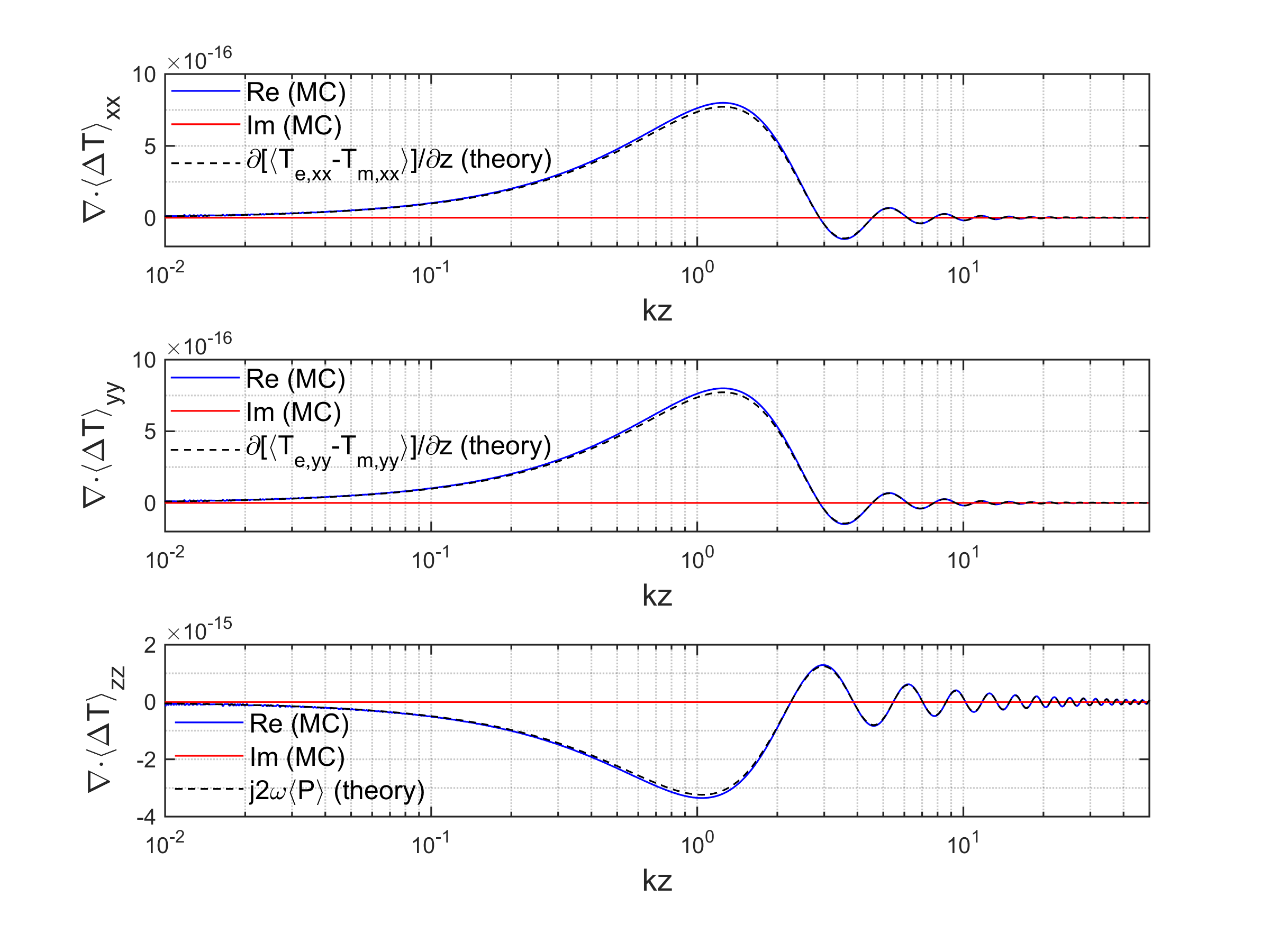
Eq. (88) also follows more directly by substituting (25) and (27) into (57), which yields Δ​Tz​z=j0​(2​k​z)\Delta{T}_{zz}=j_{0}(2kz), and applying (49). To illustrate and validate these results, Figs. 6 and 922 2 The transverse diagonal elements (α=x,y\alpha=x,y; cf. top two plots in Fig. 9) are only relevant in configurations for which ∇x{\nabla}_{x} and/or ∇y{\nabla}_{y} are also nonzero, e.g., when one or more additional adjacent boundaries are perpendicular to 1¯x\underline{1}_{x} or 1¯y\underline{1}_{y}. show ⟨Δ​Tα​α​(k​z)⟩=Δ⟨Te,α​α​(k​z)⟩−⟨Tm,α​α​(k​z)⟩\langle\Delta T_{\alpha\alpha}(kz)\rangle\stackrel{{\scriptstyle\Delta}}{{=}}\langle{T}_{e,\alpha\alpha}(kz)\rangle-\langle{T}_{m,\alpha\alpha}(kz)\rangle and their divergence, respectively. The latter Figure confirms (88) for α=z\alpha=z and (85) for arbitrary α\alpha.

Refer to caption
Fig. 9: Spatial gradients of average differential EM stress components ∇¯⋅⟨Δ​T¯¯⟩\underline{\nabla}\cdot\langle\Delta\underline{\underline{T}}\rangle [in units J/m4 or N/m3] as a function of height k​zkz above a PEC boundary and ⟨ℰ0′2⟩=⟨ℰ0′′2⟩=10−4\langle{{\cal E}^{\prime}_{0}}^{2}\rangle=\langle{{\cal E}^{\prime\prime}_{0}}^{2}\rangle=10^{-4} (V/m)2 at f=100f=100 MHz. Blue solid: MC real part, red solid: MC imaginary part, black dashed: theoretical ∂⟨Te,α​α−Tm,α​α⟩/∂z\partial\langle{T}_{e,\alpha\alpha}{-}{T}_{m,\alpha\alpha}\rangle/\partial z for α=x,y,z\alpha=x,y,z [eq. (85)].

IV-C Relation Between EM Stress and Energy

For deterministic fields, substitution of (58) into (44) enables the second-order spatial derivatives (curvatures) of the radiation stress components to be related to the EM energy imbalance Um−UeU_{m}-U_{e} (or the second-order time derivative of the total energy, for general time-dependent fields) without recourse to the LM or power, viz.,

j​ω​∇¯⋅P¯=k2​(Um−Ue)=∇¯⋅(∇¯⋅T¯¯)\displaystyle{\rm j}\omega\underline{\nabla}\cdot\underline{P}=k^{2}(U_{m}-U_{e})=\underline{\nabla}\cdot(\underline{\nabla}\cdot\underline{\underline{T}}) (90)

where ∇¯⋅(∇¯⋅T¯¯)=∂2Tz​z/∂z2\underline{\nabla}\cdot(\underline{\nabla}\cdot\underline{\underline{T}})=\partial^{2}T_{zz}/\partial z^{2} in the present configuration. For an averaged random field, the corresponding identity follows from (50) and (65) as

∇¯⋅⟨∇¯⋅T¯¯⟩−k2​(⟨Um⟩−⟨Ue⟩)=0.\displaystyle\underline{\nabla}\cdot\langle\underline{\nabla}\cdot\underline{\underline{T}}\rangle-k^{2}(\langle U_{m}\rangle-\langle U_{e}\rangle)=0. (91)

Hence ⟨∇¯⋅∇¯⋅T¯¯⟩=∇¯⋅⟨∇¯⋅T¯¯⟩\langle\underline{\nabla}\cdot\underline{\nabla}\cdot\underline{\underline{T}}\rangle=\underline{\nabla}\cdot\langle\underline{\nabla}\cdot\underline{\underline{T}}\rangle but ∇¯⋅⟨∇¯⋅T¯¯⟩≠∇¯⋅∇¯⋅⟨T¯¯⟩=0\underline{\nabla}\cdot\langle\underline{\nabla}\cdot\underline{\underline{T}}\rangle\not=\underline{\nabla}\cdot\underline{\nabla}\cdot\langle\underline{\underline{T}}\rangle=0 in view of the foregoing analysis, except asymptotically for k​z→+∞kz\rightarrow+\infty or at discrete locations and frequencies k​zskz_{s} at which the dispersion vanishes. In terms of the individual electric and magnetic average stresses and energies, (91) with (88) degenerates into separate equations, viz.,

∇¯⋅∇¯⋅⟨T¯¯(e)​(m)⟩±k2​⟨U(e)​(m)⟩=0\displaystyle\underline{\nabla}\cdot\underline{\nabla}\cdot\langle\underline{\underline{T}}_{(e)(m)}\rangle\pm k^{2}\langle U_{(e)(m)}\rangle=0 (92)

where the upper and lower signs refer to (⟨T¯¯e⟩,⟨Ue⟩)(\langle\underline{\underline{T}}_{e}\rangle,\langle U_{e}\rangle) and (⟨T¯¯m⟩,⟨Um⟩)(\langle\underline{\underline{T}}_{m}\rangle,\langle U_{m}\rangle), respectively.

V Conclusion

The average LM (20) and AM (21) (and the corresponding linear and angular power flux densities) of a random field near a PEC boundary exhibit a dependence on the electric distance k​zkz that contains similarities as well as differences compared to the dependence of the average electric or magnetic energy densities (24)–(27). Similar to the energy, the strength of the average momentum and power decays with increasing distance in a damped oscillatory manner and vanishes far away from the boundary. By contrast, the average momentum and power flux vanish on the boundary itself, their rate of decay with k​zkz is different, and their asymptotic deep values are attained at values of k​zkz in (23) that are interleaved with (i.e., spaced by approximately π/4\pi/4 from) those for the total energy density (28). As an application to reverberation chambers, it was shown that by specifying a maximum tolerable deviation (nonuniformity) of the average boundary power or energy from its asymptotic free-space value, a performance based metric for the size of the working volume of a chamber can be defined and calculated via (43).

The Poynting theorem for conservation between energy imbalance and power flux in the absence of ohmic losses was found to remain satisfied for their (arithmetic) statistical averages in the case of random fields near a PEC plane, extending its validity beyond deterministic fields to (50). Conservation of the average LM and AM can be expressed either for the average flux of the full EM stresses (65) and its moment (66), or in terms of the flux of electric or magnetic stress (86) or their difference (88), and their moments (87) and (89), respectively. The average EM energy imbalance and stress are directly related as (91) or individually as (92).

As a final comment, LM and AM of random fields were found to exhibit a partial and statistical behaviour, rather than being an all-or-nothing property in the case of deterministic fields. This is similar to other wave characteristics of inhomogeneous random fields, in particular for the degree of polarization [18], [19]. This is not surprising in view of the fact that polarization content is already comprised as SAM within AM (8).

References

  • [1] J. H. Poynting, “The wave motion of a revolving shaft, and a suggestion as to the angular momentum in a beam of circularly polarised light,” Proc. R. Soc. Lond., Ser. A, vol. 82, pp. 560–567, 1909.
  • [2] R. Beth, “Mechanical detection and measurement of the angular momentum of light,” Phys. Rev., vol. 50, pp. 115–125, 1936.
  • [3] L. Allen, M. W. Beijersbergen, R. J. C. Spreeuw, and J. P. Woerdman, “Orbital angular-momentum of light and the transformation of Laguerre–Gaussian laser modes,” Phys. Rev. A, vol. 45, pp. 8185–8189, 1992.
  • [4] B. Thidé, F. Tamburini, H. Then, C. G. Someda, and R. A. Ravanelli, “The physics of angular momentum radio,” arXiv:1410.4268v3, 2015.
  • [5] G. Ya. Slepyan, A. Boag, V. Mordachev, E. Sinkevich, S. Maksimenko, P. Kuzhir, G. Miano, M. E. Portnoi, and A. Maffucci, “Nanoscale electromagnetic compatibility: quantum coupling and matching in nanocircuits,” IEEE Trans. Electromagn. Compat., vol. 57, no. 6, pp. 1645–1654, Dec. 2015.
  • [6] M. Migliaccio, G. Gradoni, and L. R. Arnaut, “Electromagnetic reverberation: the legacy of Paolo Corona,” IEEE Trans. Electromagn. Compat., vol. 58, no. 3, pp. 643–652, Jun. 2016.
  • [7] J. M. Dunn, “Local, high-frequency analysis of the field in a mode-stirred chamber,” IEEE Trans. Electromagn. Compat., vol. 32, no. 1, pp. 53–58, Feb. 1990.
  • [8] L. R. Arnaut and P. D. West, “Electromagnetic reverberation near a perfectly conducting boundary,” IEEE Trans. Electromagn. Compat., vol. 48, no. 2, pp. 359–371, May 2006.
  • [9] L. R. Arnaut, “Spatial correlation functions of inhomogeneous random electromagnetic fields,” Phys. Rev. E, vol. 73, no. 3, 036604, Mar. 2006.
  • [10] J. D. Jackson, Classical Electrodynamics. 2nd ed. Wiley: New York, NY, 1975.
  • [11] J. A. Kong, Electromagnetic Wave Theory. 2nd ed. Wiley: New York, NY, 1990.
  • [12] M. V. Berry, “Optical currents,” J. Opt. A., vol. 11, 094001, 2009.
  • [13] D. A. Hill, Electromagnetic Theory of Reverberation Chambers. NIST Techn. Note 1506, U.S. Dept. of Commerce, Boulder, CO, Dec. 1998.
  • [14] M. Schröder, “Eigenfrequenzstatistik und Anregungsstatistik in Räumen: Modellversuche mit elektrischen Wellen,” Acustica, vol. 4, pp. 456–468, 1954.
  • [15] S. R. de Groot, The Maxwell Equations. North-Holland: Amsterdam, 1969.
  • [16] L. R. Arnaut, “Probability distribution of random electromagnetic fields in the presence of a semi-infinite isotropic medium,” Radio Sci., vol. 42, RS3001, 2007.
  • [17] G. B. Arfken, H. J. Weber, and F. E., Harris, Mathematical Methods for Physicists. 7th ed. Academic: Waltham, MA, 2013.
  • [18] L. R. Arnaut, “Compound exponential distributions for undermoded reverberation chambers,” IEEE Trans. Electromagn. Compat., vol. 44, no. 3, pp. 442–457, Aug. 2002.
  • [19] M. Migliaccio, J. J. Gil, A. Sorrentino, F. Nunziata, and G. Ferrara, “The polarization purity of the electromagnetic field in a reverberating chamber,” IEEE Trans. Electromagn. Compat., vol. 58, no. 3, pp. 694–700, Jun. 2016.
  • [20] I. V. Lindell, Methods for Electromagnetic Field Analysis. Clarendon: Oxford, U.K., 1992.

Appendix: Maxwell Stress Dyadic for Time-Harmonic Random Fields

The Maxwell stress dyadic is usually formulated in the time domain as (e.g., [10, Sec. 6.8])

T¯¯​(r¯,t)=Δϵ0​E¯​E¯+μ0​H¯​H¯−12​(ϵ0​E¯2+μ0​H¯2)​I¯¯.\displaystyle\underline{\underline{{\rm T}}}(\underline{r},t)\stackrel{{\scriptstyle\Delta}}{{=}}\epsilon_{0}\underline{{\rm E}}\,\underline{{\rm E}}+\mu_{0}\underline{{\rm H}}\,\underline{{\rm H}}-\frac{1}{2}\left(\epsilon_{0}\underline{{\rm E}}^{2}+\mu_{0}\underline{{\rm H}}^{2}\right)\underline{\underline{I}}. (93)

With an assumed exp⁡(j​ω​t)\exp({\rm j}\omega t) dependence, the corresponding expression for the complex T¯¯​(r¯,ω)\underline{\underline{T}}(\underline{r},\omega) for a time harmonic random field (OPENE¯,H¯,ω)\underline{E},\underline{H},\omega) can be derived as follows. First, consider excitation by a single plane wave (OPENℰ¯,ℋ¯,k¯)\underline{{\cal E}},\underline{{\cal H}},\underline{k}) from the angular spectrum of (OPENE¯,H¯)\underline{E},\underline{H}). Being a sum of products of complex field quantities, the complex Lorentz force can be written as

ℱ¯​(r¯,k¯)=12​(ϱ​ℰ¯∗+𝒥¯×ℬ¯∗).\displaystyle\underline{{\cal F}}(\underline{r},\underline{k})=\frac{1}{2}\left(\varrho\underline{{\cal E}}^{*}+\underline{{\cal J}}\times\underline{{\cal B}}^{*}\right). (94)

Applying Gauss’s and Ampère’s laws to express ϱ\varrho and 𝒥¯\underline{{\cal J}} in terms of their source fields gives

ℱ¯=12​[(∇¯⋅𝒟¯)​ℰ¯∗+(∇¯×ℋ¯)×ℬ¯∗−j​ω​𝒟¯×ℬ¯∗].\displaystyle\underline{{\cal F}}=\frac{1}{2}\left[(\underline{\nabla}\cdot\underline{{\cal D}})\underline{{\cal E}}^{*}+(\underline{\nabla}\times\underline{{\cal H}})\times\underline{{\cal B}}^{*}-{\rm j}\omega\underline{{\cal D}}\times\underline{{\cal B}}^{*}\right]. (95)

The last term in (95) equals −j​ω​𝒫¯-{\rm j}\omega\underline{{\cal P}}. Using dyadic algebra and the vector identity ℋ¯∗×(∇¯×ℋ¯)=∇¯​(ℋ¯∗⋅ℋ¯)−(∇¯⋅ℋ¯∗)​ℋ¯=∇¯​|ℋ¯|2−∇¯⋅(ℋ¯∗​ℋ¯)\underline{{\cal H}}^{*}\times(\underline{\nabla}\times\underline{{\cal H}})=\underline{\nabla}(\underline{{\cal H}}^{*}\cdot\underline{{\cal H}})-(\underline{\nabla}\cdot\underline{{\cal H}}^{*})\underline{{\cal H}}=\underline{\nabla}\,|\underline{{\cal H}}|^{2}-\underline{\nabla}\cdot(\underline{{\cal H}}^{*}\underline{{\cal H}}), this yields in vacuum

ℱ¯\displaystyle\underline{{\cal F}} =\displaystyle= 12[ϵ0∇¯⋅(ℰ¯ℰ¯∗)+μ0∇¯⋅(ℋ¯∗ℋ¯)\displaystyle\frac{1}{2}\left[\epsilon_{0}\underline{\nabla}\cdot(\underline{{\cal E}}\,\underline{{\cal E}}^{*})+\mu_{0}\underline{\nabla}\cdot(\underline{{\cal H}}^{*}\underline{{\cal H}})\right. (96)
−μ0∇¯⋅(|ℋ¯|2I¯¯)]−jω𝒫¯=0¯.\displaystyle\left.-\mu_{0}\underline{\nabla}\cdot(|\underline{{\cal H}}|^{2}\underline{\underline{I}})\right]-{\rm j}\omega\underline{{\cal P}}=\underline{0}.

Expressing j​ω​𝒫¯{\rm j}\omega\underline{{\cal P}} as ∇¯⋅𝒯¯¯\underline{\nabla}\cdot\underline{\underline{{\cal T}}} in view of (58) gives

𝒯¯¯​(r¯,k¯)=12​(ϵ0​ℰ¯​ℰ¯∗+μ0​ℋ¯∗​ℋ¯−μ0​|ℋ¯|2​I¯¯).\displaystyle\underline{\underline{{\cal T}}}(\underline{r},\underline{k})=\frac{1}{2}\left(\epsilon_{0}\underline{{\cal E}}\,\underline{{\cal E}}^{*}+\mu_{0}\underline{{\cal H}}^{*}\underline{{\cal H}}-\mu_{0}|\underline{{\cal H}}|^{2}\underline{\underline{I}}\right). (97)

This expression for 𝒯¯¯\underline{\underline{{\cal T}}} is dual-asymmetric because (94) is as such. Formally applying ℋ=ℰ/η0{\cal H}={\cal E}/\eta_{0} enables the last term in (97) to be dual-symmetrized [20, sec. 4.2] as μ0​|ℋ¯|2​I¯¯=(ϵ0​|ℰ¯|2+μ0​|ℋ¯|2)​I¯¯/2\mu_{0}|\underline{{\cal H}}|^{2}\underline{\underline{I}}=\left(\epsilon_{0}|\underline{{\cal E}}|^{2}+\mu_{0}|\underline{{\cal H}}|^{2}\right)\underline{\underline{I}}/2. Spherical integration of each dyad ℰα​ℰβ∗{\cal E}_{\alpha}{\cal E}^{*}_{\beta} and ℋα∗​ℋβ{\cal H}^{*}_{\alpha}{\cal H}_{\beta} according to (III-A) finally results in the stress dyadic for the time-harmonic random field as

T¯¯​(r¯,ω)\displaystyle\underline{\underline{T}}(\underline{r},\omega) =\displaystyle= 12[ϵ0E¯E¯∗+μ0H¯∗H¯\displaystyle\frac{1}{2}\left[\epsilon_{0}\underline{E}\,\underline{E}^{*}+\mu_{0}\underline{H}^{*}\underline{H}\right. (98)
−12(ϵ0|E¯|2+μ0|H¯|2)I¯¯].\displaystyle\left.-\frac{1}{2}\left(\epsilon_{0}|\underline{E}|^{2}+\mu_{0}|\underline{H}|^{2}\right)\underline{\underline{I}}\right].