跳到论文正文
W Papers独立论文阅读器 arXiv:1907.09153 论文正文 计算阅读时间 · 0%
引用这篇论文根据当前论文元数据生成,正式投稿前建议核对。


License: arXiv.org perpetual non-exclusive license
arXiv:1907.09153v3 [cond-mat.str-el] 16 Oct 2019

Ground-state atlas of a three-dimensional semimetal in the quantum limitPreprint: APS/123-QED

Zhiming Pan Affiliation: International Center for Quantum Materials, School of Physics, Peking University, Beijing 100871, China Affiliation: Collaborative Innovation Center of Quantum Matter, Beijing 100871, China    Ryuichi Shindou Email: rshindou@pku.edu.cn Affiliation: International Center for Quantum Materials, School of Physics, Peking University, Beijing 100871, China Affiliation: Collaborative Innovation Center of Quantum Matter, Beijing 100871, China
August 11, 2026
Abstract

An interplay between electron correlation and reduced dimensionality due to the Landau quantization gives rise to exotic electronic phases in three-dimensional semimetals under high magnetic field. Using an unbiased theoretical method, we clarify for the first time comprehensive ground-state phase diagrams of a three-dimensional semimetal with a pair of electron and hole pockets in the quantum limit. For the electron interaction, we consider either screened Coulomb repulsive interaction or an attractive electron-electron interaction mediated by a screened electron-phonon coupling, where a screening length is generally given by a dimensionless constant times magnetic length ll. By solving the parquet RG equation numerically and employing a mean-field argument, we construct comprehensive ground-state phase diagrams of the semimetal in the quantum limit for these two cases, as a function of the Fermi wave length and the screening length (both normalized by ll). In the repulsive interaction case, the ground state is either excitonic insulator (EI) in strong screening regime or Ising-type spin density wave in weak screening regime. In the attractive interaction case, the ground state is either EI that breaks the translational symmetries (strong screening regime), topological EI, charge Wigner crystal (intermediate screening regime), plain charge density wave or possible non-Fermi liquid (weak screening regime). We show that the topological EI supports a single copy of massless Dirac fermion at its side surface, and thereby exhibit a H⟂\sqrt{H_{\perp}}-type surface Shubnikov-de Haas (SdH) oscillation in in-plane surface transports as a function of a canted magnetic field H⟂H_{\perp}. Armed with these theoretical knowledge, we discuss implications of recent transport experiments on graphite under the high field.

I introduction

One of the fundamental challenge in condensed matter physics is a realization of three-dimensional unconventional electronic phases in the quantum limit halperin87. Recent experimental discoveries of Dirac, Weyl and nodal Dirac semimetal materials weyl-dirac18 lead to growing research interests on novel quantum transports and quantum phase transitions under high magnetic field in these new compounds tang19; zhang19; fujioka19; zhang17; ramshaw18 as well as celebrated semimetal compounds such as bismuth zhu12; zhu17a and graphite fauque13; zhu19; arnold17; leboeuf17. In fact, these semimetallic compounds under the high field often exhibit low-temperature metal-insulator transitions within wide ranges of the field tang19; fujioka19; yaguchi09; fauque13; akiba15; arnold17; leboeuf17; zhu17b; taen18; zhu19.

The quantizing effect of the strong magnetic field confines electrons into cyclotron motions in the Landau levels, while the electron’s kinetic energy along the field direction remains unaffected. This leaves the system with pristine one-dimensional momentum-energy dispersions along the field, making the system extremely sensitive to various instabilities gruner00. Previous theories proposed a number of spontaneous symmetry broken (SSB) phases as well as non-Fermi liquid phaseyakovenko93. The SSB phases proposed include charge-density wave halperin87; macdonald87; celli65; lee69; fukuyama78; yoshioka81; tesanovic87; zhang17, three-dimensional quantum Hall halperin87; balents96; bernevig07; zhang17, charge-Wigner crystal kleppmann75; fukuyama78; biagini01; tsai02a; tsai02b; alicea09, spin-density wavetakahashi94; takada98; yaguchi09; pan18, excitonic insulator fenton68; jerome67; pan18; song17; pan18, valley-density wave, and three-dimensional topological excitonic insulator pan18. Recent theoretical efforts on Dirac and Weyl semimetal models can be found in Ref. song17; trescher17. In spite of these efforts during last decades, indentities of the low-temperature insulating phases in the experiments are still veiled in mystery due to a lack of comprehensive microscopic theory based on an unbiased theoretical method.

An electronic state of the prototypical semimetal materials can be captured by a pair of electron and hole band. Under the magnetic field (∥\parallel zz), the electron/hole’s motions in the x​yxy plane are confined into clockwise/anticlockwise cyclotron orbits around the field respectively. The counter-propagating cyclotron motion in the x​yxy plane inspires an ‘electron-hole’ analogy of the two-dimensional quantum spin Hall physics qi11; hasan10. The one-dimensional dispersions along zz of the electron and hole bands go across the Fermi level at several Fermi points in the Brillouin zone. The experimental Hall conductivity measurements conclude that the relevant semimetal material within the relevant field regime yaguchi09; fauque13; akiba15; arnold17; leboeuf17; zhu17b; taen18; zhu19 are in the charge neutrality region, where electron and hole densities compensate with each other completely uji98; kopelevich09; kumar10; akiba15; pan18; zhu19. Thereby, to uncover the identities of the low-temperature insulator phases in the experiments yaguchi09; fauque13; akiba15; arnold17; leboeuf17; zhu17b; taen18; zhu19; liang19, it is vital to understand a ground-state phase diagram of a microscopic Hamiltonian for the semimetal material in the quantum limit at their charge neutrality point.

Figure 1: Electronic phase diagram of a semimetal model in the quantum limit at the charge neutrality point in the presence of the repulsive Coulomb interaction. The phase diagram is obtained from numerical solutions of the parquet RG equations. The vertical axis is B≡2​log10⁡(2​kF​l)B\equiv 2\log_{10}(2k_{F}l) [2​kF2k_{F} is a distance between the right and left Fermi points along the field, and ll is the magnetic length]. The horizontal axis is log10⁡A\log_{10}A, where A\sqrt{A} is the screening length divided by the magnetic length. We set A=A′A=A^{\prime}; see the main text. Within the RPA, AA and A′A^{\prime} are evaluated as in Eqs. (53,54) respectively.
Figure 2: Electronic phase diagram of a semimetal model in the quantum limit at the charge neutrality point in the presence of the electron-phonon interaction (A=A′A=A^{\prime}). The phase diagram is obtained from numerical solutions of the parquet RG equations for the semimetal model with an effective attractive electron-electron interaction, Eq. (3). The vertical axis is B≡2​log10⁡(2​kF​l)B\equiv 2\log_{10}(2k_{F}l). The horizontal axis is log10⁡A\log_{10}A.

In this paper, using an unbiased theoretical method, we clarify the comprehensive ground-state phase diagrams of a prototype model for a three-dimensional semimetal under the magnetic field HH (∥z\parallel\!\ z). The semimetal model has a pair of electron pocket with ↑\uparrow spin and hole pocket with ↓\downarrow spin. We study two limiting cases at the charge neutrality point, (i) the model with screened Coulomb interaction and (ii) the model with an effective attractive interaction mediated by the screened electron-phonon interaction. We rederive parquet renormalization group (RG) equations, that was originally given by Brazovskii  abrikosov70; brazovskii72; yakovenko93, solve numerically the parquet RG equations, and complete the ground-state electronic phase diagrams for these two cases. The ground-state phase diagrams thus obtained exhibit rich phase diagram structures as a function of three important length scales in the system, (α\alpha) magnetic length l≡ℏ/e​Hl\equiv\sqrt{\hbar/eH} , (β\beta) Fermi wave length (along the field) 2​π/(2​kF)2\pi/(2k_{F}), and (γ\gamma) screening length of the long-range Coulomb interaction, A​l\sqrt{A}l [see Eq. (1) for the definition of a dimensionless parameter AA, see Eq. (53) for its RPA evaluation]. In the repulsive interaction case, we found that the ground state is either Ising-type spin density wave phase or excitonic insulator (EI) phase (Fig. 1). In the attractive interaction case, we found that the ground state is either charge Wigner crystal phase, charge density wave phase, possible non-Fermi liquid yakovenko93 phase, EI phase that breaks the translational symmetry within the x​yxy plane or three-dimensional topological EI phase with a topological surface massless Dirac state pan18 (Fig. 2). We show in the paper that a canted magnetic field H⟂H_{\perp} splits the surface Dirac state into surface Landau levels (sLL). The result suggests that when in-plane transport in the topological EI phase is dominated by surface transport, the in-plane resistivity must show a H⟂\sqrt{H_{\perp}}-type surface Shubnikov-de Haas (SdH) oscillation under the canted magnetic field.

I.1 highlight of the paper

In the next section, we introduce a model Hamiltonian for the semimetal material in the quantum limit, where a pair of the electron pocket with ↑\uparrow spin and hole pocket with ↓\downarrow spin go across the Fermi level at pz=±kFp_{z}=\pm k_{F} at the charge neutrality point [pzp_{z} is momentum along the field direction]. By using the RPA approximation, we discuss in Sec. III how the long-range Coulomb interaction V⁡(𝒓)≡e2/ε​rV({\bm{r}})\equiv e^{2}/{\varepsilon r} is screened by a density fluctuation at pz=0p_{z}=0 and a fast mode of the density fluctuation at pz=2​kFp_{z}=2k_{F}. The screened Coulomb interactions thus obtained take the following forms in the momentum space tsvelik18,

V⁡(q⟂,pz≃0)\displaystyle V(q_{\perp},p_{z}\simeq 0) =4​π​e2​l2ε​1q⟂2​l2+1A​e−12​q⟂2​l2,\displaystyle=\frac{4\pi e^{2}l^{2}}{\varepsilon}\frac{1}{q^{2}_{\perp}l^{2}+\frac{1}{A}e^{-\frac{1}{2}q^{2}_{\perp}l^{2}}}, (1)
V⁡(q⟂,pz≃2​kF)\displaystyle V(q_{\perp},p_{z}\simeq 2k_{F}) =4​π​e2​l2ε​1(q⟂2+4​kF2)​l2+1A′​e−12​q⟂2​l2,\displaystyle=\frac{4\pi e^{2}l^{2}}{\varepsilon}\frac{1}{(q^{2}_{\perp}+4k^{2}_{F})l^{2}+\frac{1}{A^{\prime}}e^{-\frac{1}{2}q^{2}_{\perp}l^{2}}}, (2)

where q⟂q_{\perp} is momentum within the x​yxy plane. Here two dimensionless parameters 1/A1/A and 1/A′1/A^{\prime} are nothing but bare polarization functions associated with the density fluctuation at pz=0p_{z}=0 and the fast mode of the density fluctuation at pz=2​kFp_{z}=2k_{F} respectively. Eq. (1) especially indicates that the screening length of the long-range Coulomb interaction is given by the magnetic length times the dimensionless parameter A\sqrt{A}; larger/smaller AA stands for the weak/strong screening respectively.

The polarization function associated with the slow density fluctuation at pz=2​kFp_{z}=2k_{F} as well as the polarization function for an excitonic fluctuation have logarithmic singularities abrikosov70; brazovskii72. These singularities indicate several competing instabilities in the semimetal model at lower temperature. To identify the most dominant instability in the model within a controlled theoretical framework, we rederive in Sec. IV the one-loop parquet renormalization group (RG) equations, where the slow 2​kF2k_{F} density fluctuation as well as other fluctuations with the logarithmic singularity are taken into account on the same footing brazovskii72; zheleznyak97. Using the screened Coulomb interaction [Eqs. (1,2)] as an ‘initial’ interaction form for the RG equations, we solve the parquet RG equations numerically and identify the most relevant fluctuations (instabilities) at lower temperature for different values of AA, A′A^{\prime} and 2​kF​l2k_{F}l [an overall factor of V⁡(q⟂,pz)V(q_{\perp},p_{z}), (4​π​e2​l2)/ε(4\pi e^{2}l^{2})/\varepsilon, can be absorbed into a RG scale change at the one-loop RG equation; it does not change the phase diagram]. By combining mean-field arguments with the numerical RG solutions, we construct in Sec. V a comprehensive ground-state phase diagram in the presence of the repulsive Coulomb interaction (Fig. 1).

As the complimentary aspect for the semimetal in the quantum limit, we also study in Sec. VI an effect of electron-phonon interaction in the semimetal model under high magnetic field. Thereby, we employ a correspondence between an electron-phonon coupled system and a system with an electron-electron interaction, and adopt an effective attractive electron-electron interaction fetter03; mahan00. The effective interaction is mediated by the screened Coulomb interaction between electron and (acoustic) phonon, and thereby it takes the following form in the momentum space,

Veff​(q⟂,pz)=−ρ0M​c2​(4​π​Z​e2​l2ε​1(q⟂2+pz2)​l2+1A​e−12​q⟂2​l2)2\displaystyle V_{\rm eff}(q_{\perp},p_{z})=-\frac{\rho_{0}}{Mc^{2}}\bigg(\frac{4\pi Ze^{2}l^{2}}{\varepsilon}\frac{1}{(q^{2}_{\perp}+p^{2}_{z})l^{2}+\frac{1}{A}e^{-\frac{1}{2}q^{2}_{\perp}l^{2}}}\bigg)^{2} (3)

Here ZZ and cc are an electron valence of positively charged nucleus ion and a sound velocity of the acoustic phonon respectively, ρ0\rho_{0} and MM are the density of the charged nucleus ions and a mass of the ion respectively. To clarify possible instabilities in the semimetal model in the presence of the electron-phonon interaction, we use this effective attractive interaction [Eq. (3)] as an initial interaction form for the parquet RG equations, and solve the RG equations numerically for different values of AA, A′A^{\prime} and 2​kF​l2k_{F}l. The numerical solutions in combination with mean-field arguments gives out a comprehensive ground-state phase diagram in the presence of the effective attractive interaction (Fig. 2).

The two ground-state phase diagrams thus obtained accommodate a rich variety of electronic phases as a function of 2​kF​l2k_{F}l and AA. In the repulsive Coulomb interaction case (Sec. V), the ground state (GS) for strong screening regime [A≤3A\leq 3 for 2​kF​l≃12k_{F}l\simeq 1] is an EI phase with a spatially even-parity excitonic pairing between electron and hole at the same momentum pzp_{z}. Since the pairing is between the electron with ↑\uparrow spin and the hole with ↓\downarrow spin and it is between the electron and hole at the same spatial location within the x​yxy plane, the excitonic pairing field leads to a long-ranged ferro-type order of a X​YXY component of the spin-1 moment. For the weak screening regime [A≥3A\geq 3 for 2​kF​l≃12k_{F}l\simeq 1], the GS is a plain superposition of a density wave (DW) of the electron band with ↑\uparrow spin and a DW of the hole band with ↓\downarrow spin, that have the 2​π/(2​kF)2\pi/(2k_{F}) spatial pitch along the field. Due to the Coulomb interaction between the two DWs, a relative phase between the two DWs is locked to π\pi. Such superposition leads to an Ising-type spin density wave without any charge density modulation; the spatial pitch of the Ising-type antiferromagnetic order is 2​π/(2​kF)2\pi/(2k_{F}).

In the attractive interaction case (Sec. VI), the GS for a strong screening regime [A≤0.3A\leq 0.3 for 2​kF​l≃12k_{F}l\simeq 1] is either one of two distinct EI phases or the charge Wigner crystal. In one of the EI phases, the excitonic pairing is the spatially even-parity excitonic pairing between electron and hole at the same momentum pzp_{z}, but it is between the electron and hole at the different spatial location within the x​yxy plane [the field ∥z\parallel\!\ z]. As a result, the EI phase forms a two-dimensional texture of the X​YXY component of the spin-1 moment, breaking the translational symmetries within the x​yxy plane. The charge Wigner crystal phase breaks both the translational symmetries along the field and within the x​yxy plane by a three-dimensional texture of the charge density. The GS for the weak screening regime [A≥0.3A\geq 0.3 for 2​kF​l≃12k_{F}l\simeq 1] is either a plain charge density wave phase with the 2​π/(2​kF)2\pi/(2k_{F}) spatial pitch along the field [2​kF​l<12k_{F}l<1 for A≃1A\simeq 1] or a possible non-Fermi liquid phase [2​kF​l>12k_{F}l>1 for A≃1A\simeq 1].

The other EI phase found in the strong screening regime is a three-dimensional topological band insulator pan18; the EI phase supports a single copy of massless surface Dirac fermion state at its side surface [side surface is parallel to the field; z​xzx and y​zyz planes with the field along zz]. The EI phase in the bulk is characterized by a spatially odd-parity pairing between electron and hole at the same momentum pzp_{z} and at the same spatial location within the x​yxy plane. As a result, the EI phase does not break any translational symmetries. Besides, it has no local X​YXY component of the spin-1 moment, since the odd parity leads to a cancellation between pzp_{z} and −pz-p_{z}. Meanwhile, the odd-parity excitonic pairing in the bulk reconstructs a surface chiral Fermi arc state of the electron band with ↑\uparrow spin and that of the hole band with ↓\downarrow spin into the massless surface Dirac state with a helical spin texture. According to the so-called ‘periodic table’ of non-interacting topological insulator and topological crystalline insulator schnyder08; kitaev09; shiozaki14; kruthoff17, the EI phase can be classified as topological ‘magnetic crystalline’ insulator shiozaki14; sato19, where the massless nature of the surface Dirac fermion is protected by a magnetic point group symmetry C2,⟂​TC_{2,\perp}T [C2,⟂C_{2,\perp} denotes a π\pi rotation that changes zz to −z-z, and TT is the time reversal]. To give a physical characterization to the topological EI phase, we show in Sec. VII that a canted magnetic field H⟂H_{\perp} splits the massless surface Dirac state into surface Landau levels (sLL), whose energy spacing is proportional to H⟂​Δ0\sqrt{H_{\perp}\Delta_{0}} [Δ0\Delta_{0} is a strength of the excitonic pairing]. The result suggests that the longitudinal electric surface transport in the x​yxy direction can show a H⟂\sqrt{H_{\perp}}-type surface Shubnikov-de Haas (SdH) oscillation under the canted magnetic field. Based on these finding, we give a brief summary and discussion on the semimetal experiments in Sec. VIII.

II model Hamiltonian

An interacting electron model with a pair of electron pocket and hole pocket under high magnetic field HH (∥z\parallel z) is considered;

H^T=∫d3​𝒓​h^0​(𝒓)+12​∫d3​𝒓​d3​𝒓′​ρ^​(𝒓)​ρ^​(𝒓′)​V​(𝒓−𝒓′)\displaystyle\hat{H}_{T}=\int d^{3}{\bm{r}}\hat{h}_{0}({\bm{r}})+\frac{1}{2}\int d^{3}{\bm{r}}d^{3}{\bm{r}}^{\prime}\hat{\rho}({\bm{r}})\hat{\rho}({\bm{r}}^{\prime})V({\bm{r}}-{\bm{r}}^{\prime}) (4)
h^0(𝒓)≡∑τ=+(↑),−(↓)\displaystyle\hat{h}_{0}({\bm{r}})\equiv\sum_{\tau=+(\uparrow),-(\downarrow)}
[Ψe,τ†(𝒓){−Eg+(−ℏ2​∇z2+𝝅2)2​me−Hzτ}Ψe,τ(𝒓)\displaystyle\hskip 2.84544pt\bigg[\Psi^{\dagger}_{e,\tau}({\bm{r}})\Big\{-E_{g}+\frac{(-\hbar^{2}\nabla^{2}_{z}+{\bm{\pi}}^{2})}{2m_{e}}-H_{\rm z}\tau\Big\}\Psi_{e,\tau}({\bm{r}})
+Ψh,τ†(𝒓){Eg−(−ℏ2​∇z2+𝝅2)2​mh−Hzτ}Ψh,τ(𝒓)]\displaystyle\hskip 8.5359pt+\Psi^{\dagger}_{h,\tau}({\bm{r}})\Big\{E_{g}-\frac{(-\hbar^{2}\nabla^{2}_{z}+{\bm{\pi}}^{2})}{2m_{h}}-H_{\rm z}\tau\Big\}\Psi_{h,\tau}({\bm{r}})\bigg] (5)
(πx,πy)={(−iℏ∂x,−iℏ∂y+eHx)(−iℏ∂x−eHy,−iℏ∂y)\displaystyle(\pi_{x},\pi_{y})=\left\{\begin{array}[]{c}(-i\hbar\partial_{x},-i\hbar\partial_{y}+eHx)\\ (-i\hbar\partial_{x}-eHy,-i\hbar\partial_{y})\\ \end{array}\right.

with 𝝅≡(πx,πy){\bm{\pi}}\equiv(\pi_{x},\pi_{y}). −Eg-E_{g} and EgE_{g} are charge state energies of an electron-type and hole-type bands at the Γ\Gamma point. mem_{e} and mhm_{h} are effective masses of the electron and hole band respectively, me>0m_{e}>0 and mh>0m_{h}>0. τ=±\tau=\pm refers to the spin 1/21/2 degree of freedom (+≡↑+\equiv\!\ \uparrow, −≡↓-\equiv\!\ \downarrow). HzH_{z} denotes the Zeeman field and we assume that the gg factor is isotropic in spin and same for electron and hole band.

An electron density ρ^​(𝒓)\hat{\rho}({\bm{r}}) is a sum of the density of the electron band and that of the hole band, ρ⁡(𝒓)≡∑a=e,h∑τΨa,τ†​(𝒓)​Ψa,τ​(𝒓)\rho({\bm{r}})\equiv\sum_{a=e,h}\sum_{\tau}\Psi^{\dagger}_{a,\tau}({\bm{r}})\Psi_{a,\tau}({\bm{r}}). In this paper, we consider as the electron correlation V⁡(𝒓)V({\bm{r}}) either repulsive Coulomb interaction (Secs. III,V) or an effective attractive electron-electron interaction mediated by the screened electron-phonon interaction (Sec. VI).

Figure 3: energy-momentum dispersion of the electron and hole pocket along the field direction.

Due to the Landau quantization, the kinetic energy within a plane perpendicular to the field is quenched, where the electron band and hole band form a sequence of the Landau levels respectively;

{En,τe​(kz)=−Eg+ℏ2​pz22​me−Hz​τ+(n+12)​ℏ​ωeEn,τh​(kz)=Eg−ℏ2​pz22​mh−Hz​τ−(n+12)​ℏ​ωh\displaystyle\left\{\begin{array}[]{c}E^{e}_{n,\tau}(k_{z})=-E_{g}+\frac{\hbar^{2}p^{2}_{z}}{2m_{e}}-H_{z}\tau+\big(n+\frac{1}{2}\big)\hbar\omega_{e}\\ E^{h}_{n,\tau}(k_{z})=E_{g}-\frac{\hbar^{2}p^{2}_{z}}{2m_{h}}-H_{z}\tau-\big(n+\frac{1}{2}\big)\hbar\omega_{h}\\ \end{array}\right.

with the cyclotron frequency ℏ​ωe,h≡e​H/me,h\hbar\omega_{e,h}\equiv eH/m_{e,h}. we consider the charge neutrality region in the quantum limit, where only the lowest Landau levels (n=0n=0) with ↑\uparrow-spin electron and ↓\downarrow-spin hole bands go across the Fermi level at the same Fermi points (pz=±kFp_{z}=\pm k_{F}) , while all the others Landau levels leave the Fermi level (Fig. 3). For simplicity, we assume that the electron mass and hole mass are same, me=mh≡mm_{e}=m_{h}\equiv m, ωe=ωh≡ω\omega_{e}=\omega_{h}\equiv\omega.

We linearize the kinetic energy along the field direction around the two Fermi points. This leads to the following low-energy Hamiltonian for h^0\hat{h}_{0},

∫d3𝒓h^0(𝒓)−μN^=2πl∑σ=±∫−Λ+Λd​p2​πσvFp\displaystyle\int d^{3}{\bm{r}}\hat{h}_{0}({\bm{r}})-\mu\hat{N}=2\pi l\sum_{\sigma=\pm}\int^{+\Lambda}_{-\Lambda}\frac{dp}{2\pi}\!\ \sigma v_{F}p
∫d⁡(l​Q)​{eσ†​(Q,p)​eσ​(Q,p)−hσ†​(Q,p)​hσ​(Q,p)}\displaystyle\hskip 5.69046pt\int d(lQ)\Big\{e^{\dagger}_{\sigma}(Q,p)e_{\sigma}(Q,p)-h^{\dagger}_{\sigma}(Q,p)h_{\sigma}(Q,p)\Big\} (10)

where the magnetic length l≡ℏ/e​Hl\equiv\sqrt{\hbar/eH} and vF=ℏ2​kFmv_{F}=\frac{\hbar^{2}k_{F}}{m}. σ=±\sigma=\pm distinguishes two Fermi points, kz=±kFk_{z}=\pm k_{F}. QQ in Eq. (10) denotes momentum within the x​yxy plane. For the ‘right-mover’ fermion with positive velocity along the field, e+​(Q,p)e_{+}(Q,p) and h−​(Q,p)h_{-}(Q,p), we use a Landau gauge with an eigenstate localized along xx-direction (xx-gauge); QQ is momentum along yy-direction, Q=kyQ=k_{y}. For the ‘left-mover’ fermion with the negative velocity, e−​(Q,p)e_{-}(Q,p) and h+​(Q,p)h_{+}(Q,p), we use the Landau gauge with an eigenstate localized along yy (yy-gauge); QQ is the momentum along xx, Q=qxQ=q_{x} yakovenko93. To be more specific, electron-band and hole-band creation operators in Eq. (5) are expanded as,

Ψe,↑​(𝒓)\displaystyle\Psi_{e,\uparrow}({\bm{r}}) =∫−Λ+Λd​p2​π​ei⁡(kF+p)​z​∫d⁡(l​ky)​ψky​(x,y)​e+​(ky,p)\displaystyle=\int^{+\Lambda}_{-\Lambda}\frac{dp}{2\pi}e^{i(k_{F}+p)z}\int d(lk_{y})\psi_{k_{y}}(x,y)e_{+}(k_{y},p)
+∫−Λ+Λd​p2​πei⁡(−kF+p)​z∫d(lqx)ϕqx(x,y)e−(qx,p),\displaystyle\hskip-19.91684pt+\int^{+\Lambda}_{-\Lambda}\frac{dp}{2\pi}e^{i(-k_{F}+p)z}\int d(lq_{x})\phi_{q_{x}}(x,y)e_{-}(q_{x},p), (11)
Ψh,↓​(𝒓)\displaystyle\Psi_{h,\downarrow}({\bm{r}}) =∫−Λ+Λd​p2​π​ei⁡(kF+p)​z​∫d⁡(l​qx)​ϕqx​(x,y)​h+​(qx,p)\displaystyle=\int^{+\Lambda}_{-\Lambda}\frac{dp}{2\pi}e^{i(k_{F}+p)z}\int d(lq_{x})\phi_{q_{x}}(x,y)h_{+}(q_{x},p)
+∫−Λ+Λd​p2​πei⁡(−kF+p)​z∫d(lky)ψky(x,y)h−(ky,p),\displaystyle\hskip-22.76228pt+\int^{+\Lambda}_{-\Lambda}\frac{dp}{2\pi}e^{i(-k_{F}+p)z}\int d(lk_{y})\psi_{k_{y}}(x,y)h_{-}(k_{y},p), (12)

with the eigenstates in the LLL,

ψky​(x,y)\displaystyle\psi_{k_{y}}(x,y) ≡1π​l​e−12​l2​(x−ky​l2)2​e−i​ky​y,\displaystyle\equiv\frac{1}{\sqrt{\sqrt{\pi}l}}e^{-\frac{1}{2l^{2}}(x-k_{y}l^{2})^{2}}e^{-ik_{y}y}, (13)
ϕqx​(x,y)\displaystyle\phi_{q_{x}}(x,y) ≡1π​l​e−12​l2​(y−qx​l2)2​ei⁡(qx−yl2)​x.\displaystyle\equiv\frac{1}{\sqrt{\sqrt{\pi}l}}e^{-\frac{1}{2l^{2}}(y-q_{x}l^{2})^{2}}e^{i(q_{x}-\frac{y}{l^{2}})x}. (14)

For later convenience, note that the xx-gauge eigenstates and yy-gauge eigenstates are transformed to each other by a Fourier transformation;

∫−∞∞d⁡(l​ky)2​π​ei​qx​ky​l2​ψky​(x,y)=ϕqx​(x,y),\displaystyle\int^{\infty}_{-\infty}\frac{d(lk_{y})}{\sqrt{2\pi}}\!\ e^{iq_{x}k_{y}l^{2}}\!\ \psi_{k_{y}}(x,y)=\phi_{q_{x}}(x,y), (15)
∫−∞∞d⁡(l​qx)2​π​e−i​qx​ky​l2​ϕqx​(x,y)=ψky​(x,y).\displaystyle\int^{\infty}_{-\infty}\frac{d(lq_{x})}{\sqrt{2\pi}}\!\ e^{-iq_{x}k_{y}l^{2}}\!\ \phi_{q_{x}}(x,y)=\psi_{k_{y}}(x,y). (16)

By substituting Eqs. (11,12) into the electron-electron interaction in Eq. (4), we obtain,

12​∫d3​𝒓​d3​𝒓′​ρ^​(𝒓)​ρ^​(𝒓′)​V​(𝒓−𝒓′)≡H1+H2,\displaystyle\frac{1}{2}\int d^{3}{\bm{r}}d^{3}{\bm{r}}^{\prime}\hat{\rho}({\bm{r}})\hat{\rho}({\bm{r}}^{\prime})V({\bm{r}}-{\bm{r}}^{\prime})\equiv H_{1}+H_{2}, (17)
H1≡12​∑μ,ν=e+,e−,h+,h−∫d​p2​π​∫d⁡(l​Q1)​∫d⁡(l​Q1′)​∫d⁡(l​Q2′)​∫d⁡(l​Q2)\displaystyle H_{1}\equiv\frac{1}{2}\sum_{\mu,\nu=e_{+},e_{-},h_{+},h_{-}}\int\frac{dp}{2\pi}\int d(lQ_{1})\int d(lQ^{\prime}_{1})\int d(lQ^{\prime}_{2})\int d(lQ_{2})
Γμ​ν​(Q1,Q1′,Q2′,Q2,I0)​∫d​p22​π​aμ†​(Q1′,p2+p)​aμ​(Q2′,p2)​∫d​p12​π​aν†​(Q1,p1−p)​aν​(Q2,p1),\displaystyle\hskip 76.82234pt\Gamma_{\mu\nu}(Q_{1},Q^{\prime}_{1},Q^{\prime}_{2},Q_{2};I_{0})\int\frac{dp_{2}}{2\pi}a^{\dagger}_{\mu}(Q^{\prime}_{1},p_{2}+p)a_{\mu}(Q^{\prime}_{2},p_{2})\!\ \int\frac{dp_{1}}{2\pi}a^{\dagger}_{\nu}(Q_{1},p_{1}-p)a_{\nu}(Q_{2},p_{1}), (18)
H2≡∑μ,ν=e,h∫d​p2​π​∫d⁡(l​Q1)​∫d⁡(l​Q1′)​∫d⁡(l​Q2′)​∫d⁡(l​Q2)\displaystyle H_{2}\equiv\sum_{\mu,\nu=e,h}\int\frac{dp}{2\pi}\int d(lQ_{1})\int d(lQ^{\prime}_{1})\int d(lQ^{\prime}_{2})\int d(lQ_{2})
Φμ​ν+⁣−​(Q1,Q1′,Q2′,Q2,I2​kF)​∫d​p22​π​aμ+†​(Q1′,p2+p)​aμ−​(Q2′,p2)​∫d​p12​π​aν−†​(Q1,p1−p)​aν+​(Q2,p1),\displaystyle\hskip 39.83368pt\Phi^{+-}_{\mu\nu}(Q_{1},Q^{\prime}_{1},Q^{\prime}_{2},Q_{2};I_{2k_{F}})\int\frac{dp_{2}}{2\pi}a^{\dagger}_{\mu_{+}}(Q^{\prime}_{1},p_{2}+p)a_{\mu_{-}}(Q^{\prime}_{2},p_{2})\!\ \int\frac{dp_{1}}{2\pi}a^{\dagger}_{\nu_{-}}(Q_{1},p_{1}-p)a_{\nu_{+}}(Q_{2},p_{1}), (19)

with a notation of

{ae+​(Q,p)≡e+​(ky,p),ae−​(Q,p)≡e−​(qx,p),ah+​(Q,p)≡h+​(qx,p),ah−​(Q,p)≡h−​(ky,p).\displaystyle\left\{\begin{array}[]{c}a_{e_{+}}(Q,p)\equiv e_{+}(k_{y},p),\\ a_{e_{-}}(Q,p)\equiv e_{-}(q_{x},p),\\ a_{h_{+}}(Q,p)\equiv h_{+}(q_{x},p),\\ a_{h_{-}}(Q,p)\equiv h_{-}(k_{y},p).\\ \end{array}\right.

H1H_{1} is a sum of all the interactions that carry the zero momentum along the field (Fig. 4(a)), while H2H_{2} is a sum of all the interactions that carry the 2​kF2k_{F} momentum along the field (Fig. 4(c)). The respective interaction potentials are given by functionals of following two ‘bare’ functions of the in-plane momentum (qx,ky)(q_{x},k_{y}),

I0​(qx,ky)\displaystyle I_{0}(q_{x},k_{y}) ≡V⁡(qx,ky,pz=0)​e−12​(qx2+ky2)​l2,\displaystyle\equiv V(q_{x},k_{y},p_{z}=0)e^{-\frac{1}{2}(q^{2}_{x}+k^{2}_{y})l^{2}}, (24)
I2​kF​(qx,ky)\displaystyle I_{2k_{F}}(q_{x},k_{y}) ≡V⁡(qx,ky,pz=2​kF)​e−12​(qx2+ky2)​l2,\displaystyle\equiv V(q_{x},k_{y},p_{z}=2k_{F})e^{-\frac{1}{2}(q^{2}_{x}+k^{2}_{y})l^{2}}, (25)

with V⁡(qx,ky,pz)≡4​π​e2ε⁡(qx2+ky2+pz2)V(q_{x},k_{y},p_{z})\equiv\frac{4\pi e^{2}}{\varepsilon(q^{2}_{x}+k^{2}_{y}+p^{2}_{z})}. Specifically, Γμ​ν\Gamma_{\mu\nu} for (μ,ν)=(e+,e+)(\mu,\nu)=(e_{+},e_{+}), (h−,h−)(h_{-},h_{-}), (e+,h−)(e_{+},h_{-}), (h−,e+)(h_{-},e_{+}), Γμ​ν\Gamma_{\mu\nu} for (μ,ν)=(e−,e−)(\mu,\nu)=(e_{-},e_{-}), (h+,h+)(h_{+},h_{+}), (e−,h+)(e_{-},h_{+}), (h+,e−)(h_{+},e_{-}), Γμ​ν\Gamma_{\mu\nu} for (μ,ν)=(e+,e−)(\mu,\nu)=(e_{+},e_{-}), (h−,h+)(h_{-},h_{+}), (e+,h+)(e_{+},h_{+}), (h−,e−)(h_{-},e_{-}), and Γμ​ν\Gamma_{\mu\nu} for (μ,ν)=(e−,e+)(\mu,\nu)=(e_{-},e_{+}), (h+,h−)(h_{+},h_{-}), (h+,e+)(h_{+},e_{+}), (e−,h−)(e_{-},h_{-}) are given by the same functionals of I0​(qx,ky)I_{0}(q_{x},k_{y}) respectively;

Γe+​e+​(k1,k1′,k2′,k2,I0)=⋯=Γh−​e+​(k1,k1′,k2′,k2,I0)\displaystyle\Gamma_{e_{+}e_{+}}(k_{1},k^{\prime}_{1},k^{\prime}_{2},k_{2};I_{0})=\cdots=\Gamma_{h_{-}e_{+}}(k_{1},k^{\prime}_{1},k^{\prime}_{2},k_{2};I_{0})
=δ⁡(k1+k1′−k2−k2′)​∫d​qx\displaystyle\hskip 17.07182pt=\delta(k_{1}+k^{\prime}_{1}-k_{2}-k^{\prime}_{2})\int dq_{x}
I0​(qx,−k1+k2)​e−i​12​qx​(k1+k2−k1′−k2′)​l2,\displaystyle\hskip 51.21504ptI_{0}(q_{x},-k_{1}+k_{2})e^{-i\frac{1}{2}q_{x}(k_{1}+k_{2}-k^{\prime}_{1}-k^{\prime}_{2})l^{2}}, (26)
Γe−​e−​(q1,q1′,q2′,q2,I0)=⋯=Γh+​e−​(q1,q1′,q2′,q2,I0)\displaystyle\Gamma_{e_{-}e_{-}}(q_{1},q^{\prime}_{1},q^{\prime}_{2},q_{2};I_{0})=\cdots=\Gamma_{h_{+}e_{-}}(q_{1},q^{\prime}_{1},q^{\prime}_{2},q_{2};I_{0})
=δ⁡(q1+q1′−q2−q2′)​∫d​ky\displaystyle\hskip 17.07182pt=\delta(q_{1}+q^{\prime}_{1}-q_{2}-q^{\prime}_{2})\int dk_{y}
I0​(q1−q2,ky)​ei​12​ky​(q1+q2−q1′−q2′)​l2,\displaystyle\hskip 51.21504ptI_{0}(q_{1}-q_{2},k_{y})e^{i\frac{1}{2}k_{y}(q_{1}+q_{2}-q^{\prime}_{1}-q^{\prime}_{2})l^{2}}, (27)
Γe+​e−​(q1,k1,k2,q2,I0)=⋯=Γh−​e−​(q1,k1,k2,q2,I0)\displaystyle\Gamma_{e_{+}e_{-}}(q_{1},k_{1},k_{2},q_{2};I_{0})=\cdots=\Gamma_{h_{-}e_{-}}(q_{1},k_{1},k_{2},q_{2};I_{0})
=ei​𝒌1∧𝒌2​l2​I0​(q1−q2,−k1+k2),\displaystyle\hskip 17.07182pt=e^{i{\bm{k}}_{1}\wedge{\bm{k}}_{2}l^{2}}I_{0}(q_{1}-q_{2},-k_{1}+k_{2}), (28)
Γe−​e+​(k1,q1,q2,k2,I0)=⋯=Γe−​h−​(k1,q1,q2,k2,I0)\displaystyle\Gamma_{e_{-}e_{+}}(k_{1},q_{1},q_{2},k_{2};I_{0})=\cdots=\Gamma_{e_{-}h_{-}}(k_{1},q_{1},q_{2},k_{2};I_{0})
=ei​𝒌1∧𝒌2​l2​I0​(q1−q2,−k1+k2),\displaystyle\hskip 17.07182pt=e^{i{\bm{k}}_{1}\wedge{\bm{k}}_{2}l^{2}}I_{0}(q_{1}-q_{2},-k_{1}+k_{2}), (29)

with

𝒌1∧𝒌2≡(k1q1)∧(k2q2)=k1​q2−q1​k2.\displaystyle{\bm{k}}_{1}\wedge{\bm{k}}_{2}\equiv\left(\begin{array}[]{c}k_{1}\\ q_{1}\\ \end{array}\right)\wedge\left(\begin{array}[]{c}k_{2}\\ q_{2}\\ \end{array}\right)=k_{1}q_{2}-q_{1}k_{2}.

Φμ​ν+⁣−\Phi^{+-}_{\mu\nu} for (μ,ν)=(e,e),(h,h)(\mu,\nu)=(e,e),(h,h), Φμ​ν+⁣−\Phi^{+-}_{\mu\nu} for (μ,ν)=(e,h)(\mu,\nu)=(e,h), and Φμ​ν+⁣−\Phi^{+-}_{\mu\nu} for (μ,ν)=(h,e)(\mu,\nu)=(h,e) are given by the following functionals of I2​kF​(qx,ky)I_{2k_{F}}(q_{x},k_{y}),

Φe​e+⁣−​(q1,k1,q2,k2,I2​kF)=Φh​h+⁣−​(k1,q1,k2,q2,I2​kF)\displaystyle\Phi^{+-}_{ee}(q_{1},k_{1},q_{2},k_{2};I_{2k_{F}})=\Phi^{+-}_{hh}(k_{1},q_{1},k_{2},q_{2};I_{2k_{F}})
=l2​ei​𝒌1∧𝒌2​l2​∫d​qx​d​ky2​π​I2​kF​(qx,ky)​ei⁡(k1−k2)​qx​l2−i⁡(q1−q2)​ky​l2,\displaystyle=l^{2}e^{i{\bm{k}}_{1}\wedge{\bm{k}}_{2}l^{2}}\int\frac{dq_{x}dk_{y}}{2\pi}I_{2k_{F}}(q_{x},k_{y})e^{i(k_{1}-k_{2})q_{x}l^{2}-i(q_{1}-q_{2})k_{y}l^{2}}, (34)
Φe​h+⁣−​(k2,k1,q1,q2,I2​kF)=l2​ei⁡(k1​q1+k2​q2)​l2​∫d​qx​d​ky2​π\displaystyle\Phi^{+-}_{eh}(k_{2},k_{1},q_{1},q_{2};I_{2k_{F}})=l^{2}e^{i(k_{1}q_{1}+k_{2}q_{2})l^{2}}\int\frac{dq_{x}dk_{y}}{2\pi}
I2​kF​(qx,ky)​ei​qx​ky​l2+i​qx​(k1−k2)​l2+i​ky​(q1−q2)​l2,\displaystyle\hskip 25.6073ptI_{2k_{F}}(q_{x},k_{y})e^{iq_{x}k_{y}l^{2}+iq_{x}(k_{1}-k_{2})l^{2}+ik_{y}(q_{1}-q_{2})l^{2}}, (35)
Φh​e+⁣−​(q1,q2,k2,k1,I2​kF)=l2​e−i⁡(k1​q1+k2​q2)​l2​∫d​qx​d​ky2​π\displaystyle\Phi^{+-}_{he}(q_{1},q_{2},k_{2},k_{1};I_{2k_{F}})=l^{2}e^{-i(k_{1}q_{1}+k_{2}q_{2})l^{2}}\int\frac{dq_{x}dk_{y}}{2\pi}
I2​kF​(qx,ky)​e−i​qx​ky​l2+i​qx​(k1−k2)​l2+i​ky​(q1−q2)​l2.\displaystyle\hskip 25.6073ptI_{2k_{F}}(q_{x},k_{y})e^{-iq_{x}k_{y}l^{2}+iq_{x}(k_{1}-k_{2})l^{2}+ik_{y}(q_{1}-q_{2})l^{2}}. (36)

For later convenience, note that these functionals can be regarded homomorphic mappings of the functions. Namely, a product between two functionals of functions ff and gg is a functional of f​gfg,

∫d⁡(l​Q)​d​(l​Q′)​Γμ​ν​(Q,Q2,Q1,Q′,f)​Γν​λ​(Q2′,Q′,Q,Q1′,g)\displaystyle\int d(lQ)d(lQ^{\prime})\Gamma_{\mu\nu}(Q,Q_{2},Q_{1},Q^{\prime};f)\Gamma_{\nu\lambda}(Q^{\prime}_{2},Q^{\prime},Q,Q^{\prime}_{1};g)
=2​π​Γμ​λ​(Q2′,Q2,Q1,Q1′,f​g),\displaystyle\hskip 19.91684pt=2\pi\Gamma_{\mu\lambda}(Q^{\prime}_{2},Q_{2},Q_{1},Q^{\prime}_{1};fg), (37)

for any μ,ν,λ=e+,e−,h+,h−\mu,\nu,\lambda=e_{+},e_{-},h_{+},h_{-}. Here a summation over ν\nu is not taken in their left-hand sides. Similarly,

∫d⁡(l​Q)​d​(l​Q′)​Φμ​ν+⁣−​(Q,Q2,Q1,Q′,f)​Φν​λ+⁣−​(Q2′,Q′,Q,Q1′,g)\displaystyle\int d(lQ)d(lQ^{\prime})\Phi^{+-}_{\mu\nu}(Q,Q_{2},Q_{1},Q^{\prime};f)\Phi^{+-}_{\nu\lambda}(Q^{\prime}_{2},Q^{\prime},Q,Q^{\prime}_{1};g)
=2​π​Φμ​λ+⁣−​(Q2′,Q2,Q1,Q1′,f​g),\displaystyle\hskip 19.91684pt=2\pi\Phi^{+-}_{\mu\lambda}(Q^{\prime}_{2},Q_{2},Q_{1},Q^{\prime}_{1};fg), (38)

for any μ,ν,λ=e,h\mu,\nu,\lambda=e,h. These homomorphic natures of the functionals are useful in the next section.

In the following, we consider Eqs. (10,17,18,19) as the prototype model Hamiltonian for a semimetal in the quantum limit at the charge neutrality point.

III screened Coulomb interaction

The interaction potentials in H1H_{1} are screened by low-energy density fluctuations at pz=0p_{z}=0, while the interaction potentials in H2H_{2} are screened by the 2​kF2k_{F} density fluctuations. The respective screened interaction comprises of a sum of the bare interaction part and an effective interaction mediated by the density fluctuations. Using the random phase approximation (Fig. 4(b,d)) with a help of the homomorphic nature of the interaction potentials, Eqs. (37,38), we can show that the screened forms for the interaction potentials Γμ​ν\Gamma_{\mu\nu} and Φμ​ν+⁣−\Phi^{+-}_{\mu\nu} take exactly the same forms as their respectively bare forms in Eqs. (18,19), except that their arguments, I0​(qx,ky)I_{0}(q_{x},k_{y}) and I2​kF​(qx,ky)I_{2k_{F}}(q_{x},k_{y}), are replaced by their screened counterparts, I¯0​(qx,ky)\overline{I}_{0}(q_{x},k_{y}) and I¯2​kF​(qx,ky)\overline{I}_{2k_{F}}(q_{x},k_{y}), respectively,

I¯0​(qx,ky)=I0​(qx,ky)1−1ℏ​∑λΠ0,λ​(ω=0)​I0​(qx,ky),\displaystyle\overline{I}_{0}(q_{x},k_{y})=\frac{I_{0}(q_{x},k_{y})}{1-\frac{1}{\hbar}\sum_{\lambda}\Pi_{0,\lambda}(\omega=0)I_{0}(q_{x},k_{y})}, (39)
I¯2​kF​(qx,ky)=I2​kF​(qx,ky)1−1ℏ​∑λΠ0,λ−⁣+​(ω=0)​I2​kF​(qx,ky).\displaystyle\overline{I}_{2k_{F}}(q_{x},k_{y})=\frac{I_{2k_{F}}(q_{x},k_{y})}{1-\frac{1}{\hbar}\sum_{\lambda}\Pi^{-+}_{0,\lambda}(\omega=0)I_{2k_{F}}(q_{x},k_{y})}. (40)

Here Π0,λ​(ω)\Pi_{0,\lambda}(\omega) denotes a bare polarization function for the pz=0p_{z}=0 density fluctuation in the right/left-mover electron band (λ=e+/−\lambda=e_{+/-}) or left/right-mover hole band (λ=h+/−\lambda=h_{+/-}). It is given by

Π0,λ​(ω=0)\displaystyle\Pi_{0,\lambda}(\omega=0) =\displaystyle=
12​π​l2∫d​p12​π{θ⁡(εF−ελ,p1)​θ​(ελ,p1+p−εF)ελ,p1−ελ,p1+p\displaystyle\hskip-22.76228pt\frac{1}{2\pi l^{2}}\int\frac{dp_{1}}{2\pi}\bigg\{\frac{\theta(\varepsilon_{F}-\varepsilon_{\lambda,p_{1}})\theta(\varepsilon_{\lambda,p_{1}+p}-\varepsilon_{F})}{\varepsilon_{\lambda,p_{1}}-\varepsilon_{\lambda,p_{1}+p}}
−θ⁡(ελ,p1−εF)​θ​(εF−ελ,p1+p)ελ,p1−ελ,p1+p},\displaystyle\hskip 14.22636pt-\frac{\theta(\varepsilon_{\lambda,p_{1}}-\varepsilon_{F})\theta(\varepsilon_{F}-\varepsilon_{\lambda,p_{1}+p})}{\varepsilon_{\lambda,p_{1}}-\varepsilon_{\lambda,p_{1}+p}}\bigg\}, (41)

with the Heaviside step function θ⁡(x)\theta(x). From Eq. (10), ελ,p−εF≡vF​p\varepsilon_{\lambda,p}-\varepsilon_{F}\equiv v_{F}p for λ=e+,h−\lambda=e_{+},h_{-} and ελ,p−εF≡−vF​p\varepsilon_{\lambda,p}-\varepsilon_{F}\equiv-v_{F}p for λ=e−,h+\lambda=e_{-},h_{+}. Noting that pp is much smaller than kFk_{F}, one obtains the bare polarization function as

Π0,λ​(ω=0)=−1(2​π​l)2​1vF,\displaystyle\Pi_{0,\lambda}(\omega=0)=-\frac{1}{(2\pi l)^{2}}\frac{1}{v_{F}}, (42)

for λ=e+,e−,h+,h−\lambda=e_{+},e_{-},h_{+},h_{-}. Π0,λ−⁣+​(ω)\Pi^{-+}_{0,\lambda}(\omega) is the bare polarization function for the 2​kF2k_{F} density fluctuation within the electron band (λ=e\lambda=e) or hole band (λ=h\lambda=h),

Π0,λ−⁣+​(ω=0)\displaystyle\Pi^{-+}_{0,\lambda}(\omega=0) =\displaystyle=
12​π​l2∫d​p12​π{θ⁡(εF−ελ−,p1)​θ​(ελ+,p1+p−εF)ελ−,p1−ελ+,p1+p\displaystyle\hskip-22.76228pt\frac{1}{2\pi l^{2}}\int\frac{dp_{1}}{2\pi}\bigg\{\frac{\theta(\varepsilon_{F}-\varepsilon_{\lambda_{-},p_{1}})\theta(\varepsilon_{\lambda_{+},p_{1}+p}-\varepsilon_{F})}{\varepsilon_{\lambda_{-},p_{1}}-\varepsilon_{\lambda_{+},p_{1}+p}}
−θ⁡(ελ−,p1−εF)​θ​(εF−ελ+,p1+p)ελ−,p1−ελ+,p1+p}.\displaystyle\hskip-8.5359pt-\frac{\theta(\varepsilon_{\lambda_{-},p_{1}}-\varepsilon_{F})\theta(\varepsilon_{F}-\varepsilon_{\lambda_{+},p_{1}+p})}{\varepsilon_{\lambda_{-},p_{1}}-\varepsilon_{\lambda_{+},p_{1}+p}}\bigg\}. (43)

From Eq. (10), ελ±,p−εF=±vF​p\varepsilon_{\lambda_{\pm},p}-\varepsilon_{F}=\pm v_{F}p for λ=e\lambda=e and ελ±,p−εF=∓vF​p\varepsilon_{\lambda_{\pm},p}-\varepsilon_{F}=\mp v_{F}p for λ=h\lambda=h.

Figure 4: (a) interaction potentials in H1H_{1}; Γμ​ν\Gamma_{\mu\nu} in Eq. (18) (μ,ν=e+,e−,h+,h−\mu,\nu=e_{+},e_{-},h_{+},h_{-}). (b) screened form of Γμ​ν\Gamma_{\mu\nu} in Eq. (18). (c) interaction potentials in H2H_{2}; Φμ​ν+⁣−\Phi^{+-}_{\mu\nu} in Eq. (19) (μ,ν=e,h\mu,\nu=e,h). (d) screened form of Φμ​ν+⁣−\Phi^{+-}_{\mu\nu} in Eq. (19), where we only include the fast mode of the 2​kF2k_{F} density fluctuation. The slow 2​kF2k_{F} density fluctuation shall be included in the parquet RG equations; see Fig. 6, e.g. the last two Feynman diagrams in the right-hand side of the first and second lines as well as the first two Feynman diagrams in the right-hand side of the fourth line.

The polarization function for 2​kF2k_{F} density fluctuation can be divided into low-energy (slow) 2​kF2k_{F} density fluctuation part and high-energy (fast) 2​kF2k_{F} density fluctuation part,

Π0,λ−⁣+(ω=0)=Π0,λ−+,s(ω=0)+Π0,λ−+,f(ω=0),\displaystyle\Pi^{-+}_{0,\lambda}(\omega=0)=\Pi^{-+,{\rm s}}_{0,\lambda}(\omega=0)+\Pi^{-+,{\rm f}}_{0,\lambda}(\omega=0), (44)
Π0,λ−+,s(ω=0)≡12​π​l2∫|p1|<Λd​p12​π{⋯},\displaystyle\Pi^{-+,{\rm s}}_{0,\lambda}(\omega=0)\equiv\frac{1}{2\pi l^{2}}\int_{|p_{1}|<\Lambda}\frac{dp_{1}}{2\pi}\bigg\{\cdots\bigg\}, (45)
Π0,λ−+,f(ω=0)≡12​π​l2∫Λ<|p1|<ΛUVd​p12​π{⋯}.\displaystyle\Pi^{-+,{\rm f}}_{0,\lambda}(\omega=0)\equiv\frac{1}{2\pi l^{2}}\int_{\Lambda<|p_{1}|<\Lambda_{\rm UV}}\frac{dp_{1}}{2\pi}\bigg\{\cdots\bigg\}. (46)

Here ΛUV\Lambda_{\rm UV} is a momentum cut off associated with the Brillouin zone boundary, while Λ\Lambda separates the slow mode from the fast mode, Λ<ΛUV\Lambda<\Lambda_{\rm UV}. The slow 2​kF2k_{F} density fluctuation part (|p1|<Λ|p_{1}|<\Lambda) leads to the logarithmic singularity at p=0p=0 zheleznyak97,

Π0,λ−+,s(ω=0)≃−1(2​π​l)21vFln(2​Λ|p|),\displaystyle\Pi^{-+,{\rm s}}_{0,\lambda}(\omega=0)\simeq-\frac{1}{(2\pi l)^{2}}\frac{1}{v_{F}}\ln\bigg(\frac{2\Lambda}{|p|}\bigg), (47)

for any λ=e,h\lambda=e,h. The singularity is a seed of the 2​kF2k_{F} DW instability in each pocket gruner00; abrikosov70; brazovskii72; yakovenko93. More generally, ‘bubble’ Feynman diagrams composed of two single-particle Green functions with opposite sign of the Fermi velocities have the same logarithmic singularity both in particle-hole and in particle-particle channels abrikosov70; brazovskii72. These logarithmic singularities suggest that the ground state of the electron-hole model at the charge neutrality point has several competing instabilities at lower temperature. To clarify the most dominant instability precisely, we thus take into account the slow 2​kF2k_{F} density fluctuation in the framework of parquet RG equations and include it as well as the other low-energy fluctuations with the logarithmic singularity on the equal footing (see the next section). Therefore, to avoid the double counting of the slow 2​kF2k_{F} density fluctuation part, we include in Eq. (40) only the high-energy (fast) 2​kF2k_{F} density fluctuation part first. This determines a form of the screened interaction. The screened interaction thus obtained is then used for an ‘initial’ interaction potential for the RG equations (Fig. 5). Finally, the low-energy (slow) 2​kF2k_{F} density fluctuation as well as other dominant low-energy fluctuations shall be included sequentially in the framework of the RG procedure (Fig. 6). For example, in Fig. 6, the last two Feynman diagrams in the right-hand side of the first and second lines as well as the first two Feynman diagrams in the right-hand side of the fourth line represents the inclusions of the slow 2​kF2k_{F} density fluctuations. The fast 2​kF2k_{F} density fluctuation part, Eq. (46), takes a constant finite value at p=0p=0,

Π0,λ−+,f(ω=0)\displaystyle\Pi^{-+,{\rm f}}_{0,\lambda}(\omega=0) ≃−1(2​π​l)2​1vF​ln⁡(ΛUVΛ),\displaystyle\simeq-\frac{1}{(2\pi l)^{2}}\frac{1}{v_{F}}\ln\bigg(\frac{\Lambda_{\rm UV}}{\Lambda}\bigg), (48)

for λ=e,h\lambda=e,h.

To summarize, we will use the following form of the screened interaction potentials as the initial interaction forms for the later parquet RG studies;

Hint\displaystyle H_{\rm int} ≡H¯1+H¯2,\displaystyle\equiv\overline{H}_{1}+\overline{H}_{2},
H¯1\displaystyle\overline{H}_{1} =12​∑μ,ν=e+,e−,h+,h−∫d​p​d​p1​d​p2(2​π)3\displaystyle=\frac{1}{2}\sum_{\mu,\nu=e_{+},e_{-},h_{+},h_{-}}\int\frac{dp\!\ dp_{1}\!\ dp_{2}}{(2\pi)^{3}}
∫d⁡(l​Q1)​d​(l​Q1′)​d​(l​Q2′)​d​(d​Q2)​Γμ​ν​(Q1,Q1′,Q2′,Q2,I¯0)\displaystyle\hskip-19.91684pt\int d(lQ_{1})d(lQ^{\prime}_{1})d(lQ^{\prime}_{2})d(dQ_{2})\!\ \Gamma_{\mu\nu}(Q_{1},Q^{\prime}_{1},Q^{\prime}_{2},Q_{2};\overline{I}_{0})
aμ†​(Q1′,p2+p)​aμ​(Q2′,p2)​aν†​(Q1,p1−p)​aν​(Q2,p1),\displaystyle\hskip-11.38092pta^{\dagger}_{\mu}(Q^{\prime}_{1},p_{2}+p)a_{\mu}(Q^{\prime}_{2},p_{2})a^{\dagger}_{\nu}(Q_{1},p_{1}-p)a_{\nu}(Q_{2},p_{1}), (49)
H¯2\displaystyle\overline{H}_{2} =∑μ,ν=e,h∫d​p​d​p1​d​p2(2​π)3\displaystyle=\sum_{\mu,\nu=e,h}\int\frac{dp\!\ dp_{1}\!\ dp_{2}}{(2\pi)^{3}}
∫d⁡(l​Q1)​d​(l​Q1′)​d​(l​Q2′)​d​(l​Q2)​Φμ​ν+⁣−​(Q1,Q1′,Q2′,Q2,I¯2​kF)\displaystyle\hskip-19.91684pt\int d(lQ_{1})d(lQ^{\prime}_{1})d(lQ^{\prime}_{2})d(lQ_{2})\Phi^{+-}_{\mu\nu}(Q_{1},Q^{\prime}_{1},Q^{\prime}_{2},Q_{2};\overline{I}_{2k_{F}})
aμ+†​(Q1′,p2+p)​aμ−​(Q2′,p2)​aν−†​(Q1,p1−p)​aν+​(Q2,p1),\displaystyle\hskip-14.22636pta^{\dagger}_{\mu_{+}}(Q^{\prime}_{1},p_{2}+p)a_{\mu_{-}}(Q^{\prime}_{2},p_{2})a^{\dagger}_{\nu_{-}}(Q_{1},p_{1}-p)a_{\nu_{+}}(Q_{2},p_{1}), (50)
I¯0​(qx,ky)=4​π​e2​l2ε​e−12​(qx2+ky2)​l2(qx2+ky2)​l2+1A​e−12​(qx2+ky2)​l2,\displaystyle\overline{I}_{0}(q_{x},k_{y})=\frac{4\pi e^{2}l^{2}}{\varepsilon}\frac{e^{-\frac{1}{2}(q^{2}_{x}+k^{2}_{y})l^{2}}}{(q^{2}_{x}+k^{2}_{y})l^{2}+\frac{1}{A}e^{-\frac{1}{2}(q^{2}_{x}+k^{2}_{y})l^{2}}}, (51)
I¯2​kF​(qx,ky)=4​π​e2​l2ε​e−12​(qx2+ky2)​l2(qx2+ky2)​l2+B+1A′​e−12​(qx2+ky2)​l2\displaystyle\overline{I}_{2k_{F}}(q_{x},k_{y})=\frac{4\pi e^{2}l^{2}}{\varepsilon}\frac{e^{-\frac{1}{2}(q^{2}_{x}+k^{2}_{y})l^{2}}}{(q^{2}_{x}+k^{2}_{y})l^{2}+B+\frac{1}{A^{\prime}}e^{-\frac{1}{2}(q^{2}_{x}+k^{2}_{y})l^{2}}} (52)

with B≡4​kF2​l2B\equiv 4k^{2}_{F}l^{2} and

1A\displaystyle\frac{1}{A} ≡−4​π​e2​l2ℏ​ε∑λ=e±,h±Π0,λ(ω=0)=4​e2ℏ​π​vF​ε,\displaystyle\equiv-\frac{4\pi e^{2}l^{2}}{\hbar\varepsilon}\sum_{\lambda=e_{\pm},h_{\pm}}\Pi_{0,\lambda}(\omega=0)=\frac{4e^{2}}{\hbar\pi v_{F}\varepsilon}, (53)
1A′\displaystyle\frac{1}{A^{\prime}} ≡−4​π​e2​l2ℏ​ε∑λ=e,hΠ0,λ−+,f(ω=0)=2​e2​ln⁡[ΛUVΛ]ℏ​π​vF​ε.\displaystyle\equiv-\frac{4\pi e^{2}l^{2}}{\hbar\varepsilon}\sum_{\lambda=e,h}\Pi^{-+,{\rm f}}_{0,\lambda}(\omega=0)=\frac{2e^{2}\ln\big[\frac{\Lambda_{\rm UV}}{\Lambda}\big]}{\hbar\pi v_{F}\varepsilon}. (54)

For simplicity, we take ln⁡(ΛUV/Λ)=2\ln(\Lambda_{\rm UV}/\Lambda)=2 henceforth and identify A′A^{\prime} with AA. For reminder, the functionals Γμ​ν\Gamma_{\mu\nu} (μ,ν=e+,e−,h+,h−\mu,\nu=e_{+},e_{-},h_{+},h_{-}) and Φμ​ν+⁣−\Phi^{+-}_{\mu\nu} (μ,ν=e,h\mu,\nu=e,h) in Eqs. (49,50) are defined in Eqs. (26,27,28,29,34, 35,36) respectively.

IV parquet renormalization group equation

The polarization function for the slow 2​kF2k_{F} density fluctuation has the logarithmic singularity [Eq. (47)]. More generally, all the ‘bubble’ diagrams composed of the two Green functions with opposite sign of the Fermi velocities have the same logarithmic singularity in both particle-hole and particle-particle channels. The presence of the logarithmic singularities in several distinct channels means competing ground-state instabilities in the semimetal model. To reveal the ground-state phase diagram of the model precisely, we thus include all the relevant fluctuations with the logarithmic singularity on the equal footing.

To this end, we derive in this section the parquet renormalization group (RG) equations abrikosov70; brazovskii72; yakovenko93, where consecutive integration of the higher-energy fermionic degree of freedom renormalizes the interaction potentials among the lower-energy fermions. The renormalization gives rise to either enhancement, suppression or convergence of the interaction potentials. By identifying the most divergent potentials among the others, we shall tell the dominant ground-state instability in the model.

Figure 5: A set of initial forms of the interaction potentials for the parquet RG equations are given by the RPA screened Coulomb interactions, Eqs. (49,50,51,52). (a) Wb​(𝒌,ξ)W_{b}({\bm{k}},\xi) at the initial RG scale (ξ=0\xi=0) that corresponds to Eq. (57), (b) Wd​(𝒌)W_{d}({\bm{k}}) at ξ=0\xi=0, corresponding to Eq. (57) (c) We​(𝒌)W_{e}({\bm{k}}) at ξ=0\xi=0, corresponding to Eq. (58) (d) Wg​(𝒌)W_{g}({\bm{k}}) at ξ=0\xi=0, corresponding to Eq. (59).

The one-loop parquet RG equations can be derived by a standard momentum shell renormalization. Thereby, we begin with a partition function of the interacting fermion model;

Z\displaystyle Z =∫𝒟​e±†​𝒟​e±​𝒟​h±†​𝒟​h±​e−S0−S1\displaystyle=\int{\cal D}e^{\dagger}_{\pm}{\cal D}e_{\pm}{\cal D}h^{\dagger}_{\pm}{\cal D}h_{\pm}e^{-S_{0}-S_{1}}
S0=\displaystyle S_{0}= ∑σ=±∫d⁡(l​ω)2​π∫|p|<Λdp∫dQ{(−iω+σvFp)\displaystyle\sum_{\sigma=\pm}\int\frac{d(l\omega)}{2\pi}\int_{|p|<\Lambda}dp\int dQ\!\ \Big\{\big(-i\omega+\sigma v_{F}p\big)
×eσ†​(Q,p,ω)​eσ​(Q,p,ω)+(−i​ω−σ​vF​p)\displaystyle\times e^{\dagger}_{\sigma}(Q,p,\omega)e_{\sigma}(Q,p,\omega)+\big(-i\omega-\sigma v_{F}p\big)
×hσ†(Q,p,ω)hσ(Q,p,ω)},\displaystyle\times h^{\dagger}_{\sigma}(Q,p,\omega)h_{\sigma}(Q,p,\omega)\Big\}, (55)
S1\displaystyle S_{1} =∫1,2,3∫d​k1​d​q1​d​k2​d​q2​ei​𝒌1∧𝒌2​Wb​(𝒌1−𝒌2)\displaystyle=\int_{1,2,3}\int dk_{1}dq_{1}dk_{2}dq_{2}\!\ \!\ e^{i{\bm{k}}_{1}\wedge{\bm{k}}_{2}}W_{b}({\bm{k}}_{1}-{\bm{k}}_{2})
e+†​(k1,1)​e−†​(q1,2)​e−​(q2,3)​e+​(k2,1+2−3)\displaystyle\hskip 8.5359pte^{\dagger}_{+}(k_{1},1)e^{\dagger}_{-}(q_{1},2)e_{-}(q_{2},3)e_{+}(k_{2},1+2-3)
+∫1,2,3∫dk1dq1dk2dq2ei​𝒌1∧𝒌2Wd(𝒌1−𝒌2)\displaystyle+\int_{1,2,3}\int dk_{1}dq_{1}dk_{2}dq_{2}\!\ \!\ e^{i{\bm{k}}_{1}\wedge{\bm{k}}_{2}}W_{d}({\bm{k}}_{1}-{\bm{k}}_{2})
h−†​(k1,1)​h+†​(q1,2)​h+​(q2,3)​h−​(k2,1+2−3)\displaystyle\hskip 8.5359pth^{\dagger}_{-}(k_{1},1)h^{\dagger}_{+}(q_{1},2)h_{+}(q_{2},3)h_{-}(k_{2},1+2-3)
+∫1,2,3∫dk1dq1dk2dq2ei​𝒌1∧𝒌2We(𝒌1−𝒌2)\displaystyle+\int_{1,2,3}\int dk_{1}dq_{1}dk_{2}dq_{2}\!\ \!\ e^{i{\bm{k}}_{1}\wedge{\bm{k}}_{2}}W_{e}({\bm{k}}_{1}-{\bm{k}}_{2})
e+†​(k1,1)​h+†​(q1,2)​h+​(q2,3)​e+​(k2,1+2−3)\displaystyle\hskip 8.5359pte^{\dagger}_{+}(k_{1},1)h^{\dagger}_{+}(q_{1},2)h_{+}(q_{2},3)e_{+}(k_{2},1+2-3)
+∫1,2,3∫dk1dq1dk2dq2ei​𝒌1∧𝒌2We(𝒌1−𝒌2)\displaystyle+\int_{1,2,3}\int dk_{1}dq_{1}dk_{2}dq_{2}\!\ \!\ e^{i{\bm{k}}_{1}\wedge{\bm{k}}_{2}}W_{e}({\bm{k}}_{1}-{\bm{k}}_{2})
h−†​(k1,1)​e−†​(q1,2)​e−​(q2,3)​h−​(k2,1+2−3)\displaystyle\hskip 8.5359pth^{\dagger}_{-}(k_{1},1)e^{\dagger}_{-}(q_{1},2)e_{-}(q_{2},3)h_{-}(k_{2},1+2-3)
+∫1,2,3∫dk1dq1dk2dq2ei⁡(k1​q1+k2​q2)Wg(𝒌1−𝒌2)\displaystyle+\int_{1,2,3}\int dk_{1}dq_{1}dk_{2}dq_{2}\!\ \!\ e^{i(k_{1}q_{1}+k_{2}q_{2})}W_{g}({\bm{k}}_{1}-{\bm{k}}_{2})
e+†​(k1,1)​h−†​(k2,2)​h+​(q2,3)​e−​(q1,1+2−3)\displaystyle\hskip 8.5359pte^{\dagger}_{+}(k_{1},1)h^{\dagger}_{-}(k_{2},2)h_{+}(q_{2},3)e_{-}(q_{1},1+2-3)
+∫1,2,3∫dk1dq1dk2dq2e−i⁡(k1​q1+k2​q2)Wg∗(𝒌1−𝒌2)\displaystyle+\int_{1,2,3}\int dk_{1}dq_{1}dk_{2}dq_{2}\!\ \!\ e^{-i(k_{1}q_{1}+k_{2}q_{2})}W^{*}_{g}({\bm{k}}_{1}-{\bm{k}}_{2})
h+†​(q1,1)​e−†​(q2,2)​e+​(k2,3)​h−​(k1,1+2−3)+⋯.\displaystyle\hskip-8.5359pth^{\dagger}_{+}(q_{1},1)e^{\dagger}_{-}(q_{2},2)e_{+}(k_{2},3)h_{-}(k_{1},1+2-3)+\cdots. (56)

Here Q=kyQ=k_{y} or qxq_{x} is rescaled by the magnetic length ll; Qnew≡Qold​lQ_{\rm new}\equiv Q_{\rm old}l. Besides, we used the following notations,

1≡(p1,ω1), 2≡(p2,ω2), 3≡(p3,ω3)\displaystyle 1\equiv(p_{1},\omega_{1}),\ \ 2\equiv(p_{2},\omega_{2}),\ \ 3\equiv(p_{3},\omega_{3})
∫1,2,3≡∫d​ω1​d​ω2​d​ω3(2​π)3∫d​p1​d​p2​d​p3(2​π)3\displaystyle\int_{1,2,3}\equiv\int\frac{d\omega_{1}\!\ d\omega_{2}\!\ d\omega_{3}}{(2\pi)^{3}}\int\frac{dp_{1}\!\ dp_{2}\!\ dp_{3}}{(2\pi)^{3}}
𝒌1≡(k1,q1),𝒌2≡(k2,q2),\displaystyle{\bm{k}}_{1}\equiv(k_{1},q_{1}),\ \ {\bm{k}}_{2}\equiv(k_{2},q_{2}),
𝒌1∧𝒌2≡k1​q2−k2​q1.\displaystyle{\bm{k}}_{1}\wedge{\bm{k}}_{2}\equiv k_{1}q_{2}-k_{2}q_{1}.

For the repulsive Coulomb interaction case, the interaction potentials in S1S_{1} are given by either some of H¯1\overline{H}_{1} or H¯2\overline{H}_{2} or their combination from Eqs. (49,50,51,52) (see Fig. 5). Namely, Wb​(𝒌)W_{b}({\bm{k}}) and Wd​(𝒌)W_{d}({\bm{k}}) are given by a sum of Eq. (28) and Eq. (34) with I0I_{0} and I2​kFI_{2k_{F}} replaced by I¯0\overline{I}_{0} and I¯2​kF\overline{I}_{2k_{F}}. We​(𝒌)W_{e}({\bm{k}}) and Wg​(𝒌)W_{g}({\bm{k}}) are given by Eq. (28) and by Eq. (36) respectively with I¯0\overline{I}_{0} and I¯2​kF\overline{I}_{2k_{F}}. To be more specific, we consider the following set of the screened interaction as the initial interaction forms of the RG equations,

Wb​(𝒌)\displaystyle W_{b}({\bm{k}}) =Wd​(𝒌)\displaystyle=W_{d}({\bm{k}})
=I¯0​(qx,ky)−∫d​qx′​d​ky′2​π​ei​ky​qx′−i​qx​ky′​I¯2​kF​(qx′,ky′),\displaystyle\hskip-34.14322pt=\overline{I}_{0}(q_{x},k_{y})-\int\frac{dq^{\prime}_{x}\!\ dk^{\prime}_{y}}{2\pi}e^{ik_{y}q^{\prime}_{x}-iq_{x}k^{\prime}_{y}}\overline{I}_{2k_{F}}(q^{\prime}_{x},k^{\prime}_{y}), (57)
We​(𝒌)\displaystyle W_{e}({\bm{k}}) =I¯0​(qx,ky),\displaystyle=\overline{I}_{0}(q_{x},k_{y}), (58)
Wg​(𝒌)\displaystyle W_{g}({\bm{k}}) =∫d​qx′​d​ky′2​π​ei​qx′​ky′+i​qx′​ky+i​ky′​qx​I¯2​kF​(qx′,ky′),\displaystyle=\int\frac{dq^{\prime}_{x}\!\ dk^{\prime}_{y}}{2\pi}e^{iq^{\prime}_{x}k^{\prime}_{y}+iq^{\prime}_{x}k_{y}+ik^{\prime}_{y}q_{x}}\overline{I}_{2k_{F}}(q^{\prime}_{x},k^{\prime}_{y}), (59)

with 𝒌≡(ky,qx){\bm{k}}\equiv(k_{y},q_{x}) and Eqs. (51,52). ``⋯"``\cdots" in Eq. (56) denotes those interaction parts that are not renormalized by others and do not renormalize others at the level of the one-loop RG equations. Such interaction parts are irrelevant in the framework of the one-loop RG analyses; we thus omit them henceforth.

Figure 6: parquet RG equations in terms of Feynman diagrams. From the top to the bottom, each line of equations correspond to Eqs. (60,61,62,63) respectively

Following the standard momentum shell renormalization process (Appendix B), we first decompose the fermionic field into fast mode (Λ−d​Λ<|p|<Λ\Lambda-d\Lambda<|p|<\Lambda) and slow mode (|p|<Λ−d​Λ|p|<\Lambda-d\Lambda) in the momentum along the field. The integration of the fast mode in the partition function leads to the renormalizations of the interaction potentials among the slow modes. This gives out a set of coupled RG equations for the interaction potentials,

d​Wb​(𝒌)d​ξ\displaystyle\frac{dW_{b}({\bm{k}})}{d\xi} =∫d​𝒌′​Wb​(𝒌′)​Wb​(𝒌−𝒌′)​(1−e−i​𝒌∧𝒌′)\displaystyle=\int d{\bm{k}}^{\prime}\!\ W_{b}({\bm{k}}^{\prime})W_{b}({\bm{k}}-{\bm{k}}^{\prime})\big(1-e^{-i{\bm{k}}\wedge{\bm{k}}^{\prime}}\big)
+∫d𝒌′Wg(𝒌′)Wg∗(𝒌−𝒌′)\displaystyle\hskip 34.14322pt+\int d{\bm{k}}^{\prime}\!\ W_{g}({\bm{k}}^{\prime})W^{*}_{g}({\bm{k}}-{\bm{k}}^{\prime}) (60)
d​Wd​(𝒌)d​ξ\displaystyle\frac{dW_{d}({\bm{k}})}{d\xi} =∫d​𝒌′​Wd​(𝒌′)​Wd​(𝒌−𝒌′)​(1−e−i​𝒌∧𝒌′)\displaystyle=\int d{\bm{k}}^{\prime}\!\ W_{d}({\bm{k}}^{\prime})W_{d}({\bm{k}}-{\bm{k}}^{\prime})\big(1-e^{-i{\bm{k}}\wedge{\bm{k}}^{\prime}}\big)
+∫d𝒌′Wg(𝒌′)Wg∗(𝒌−𝒌′)\displaystyle\hskip 34.14322pt+\int d{\bm{k}}^{\prime}\!\ W_{g}({\bm{k}}^{\prime})W^{*}_{g}({\bm{k}}-{\bm{k}}^{\prime}) (61)
d​We​(𝒌)d​ξ\displaystyle\frac{dW_{e}({\bm{k}})}{d\xi} =∫d​𝒌′​We​(𝒌′)​We​(𝒌−𝒌′)​(1−e−i​𝒌∧𝒌′)\displaystyle=\int d{\bm{k}}^{\prime}\!\ W_{e}({\bm{k}}^{\prime})W_{e}({\bm{k}}-{\bm{k}}^{\prime})\big(1-e^{-i{\bm{k}}\wedge{\bm{k}}^{\prime}}\big)
+∫d𝒌′e−i​k​q+i​k′​q+i​k​q′Wg(𝒌′)Wg∗(𝒌−𝒌′)\displaystyle\hskip-11.38092pt+\int d{\bm{k}}^{\prime}\!\ e^{-ikq+ik^{\prime}q+ikq^{\prime}}W_{g}({\bm{k}}^{\prime})W^{*}_{g}({\bm{k}}-{\bm{k}}^{\prime}) (62)
d​Wg​(𝒌)d​ξ\displaystyle\frac{dW_{g}({\bm{k}})}{d\xi} =∫d𝒌′Wg(𝒌−𝒌′){Wb(𝒌′)+Wd(𝒌′)\displaystyle=\int d{\bm{k}}^{\prime}\!\ W_{g}({\bm{k}}-{\bm{k}}^{\prime})\Big\{W_{b}({\bm{k}}^{\prime})+W_{d}({\bm{k}}^{\prime})
+e−i​k​q′−i​k′​q+i​k′​q′We(𝒌′)}\displaystyle\hskip 56.9055pt+2\!\ e^{-ikq^{\prime}-ik^{\prime}q+ik^{\prime}q^{\prime}}W_{e}({\bm{k}}^{\prime})\Big\} (63)

with 𝒌≡(k,q){\bm{k}}\equiv(k,q), 𝒌′≡(k′,q′){\bm{k}}^{\prime}\equiv(k^{\prime},q^{\prime}), and d​𝒌′≡d​k′​d​q′d{\bm{k}}^{\prime}\equiv dk^{\prime}dq^{\prime}. d​ξd\xi denotes a RG scale,

d​ξ≡1(2​π)3​l2​d​ΛvF​Λ.\displaystyle d\xi\equiv\frac{1}{(2\pi)^{3}l^{2}}\frac{d\Lambda}{v_{F}\Lambda}. (64)

In order to solve the coupled RG equations numerically, we put them in the dual-space representation by the Fourier transform of Wμ​(𝒌)W_{\mu}({\bm{k}}),

Fμ​(𝒓)≡∫d​𝒌​e−i​𝒌​𝒓​Wμ​(𝒌),\displaystyle F_{\mu}({\bm{r}})\equiv\int d{\bm{k}}e^{-i{\bm{k}}{\bm{r}}}W_{\mu}({\bm{k}}), (65)
Wμ​(𝒌)≡∫d​𝒓(2​π)2​ei​𝒌​𝒓​Fμ​(𝒓),\displaystyle W_{\mu}({\bm{k}})\equiv\int\frac{d{\bm{r}}}{(2\pi)^{2}}e^{i{\bm{k}}{\bm{r}}}F_{\mu}({\bm{r}}), (66)

for μ=b,d,e,g\mu=b,d,e,g with

F~g​(𝒓)≡e−i​rx​ry​Fg​(𝒓),\displaystyle\tilde{F}_{g}({\bm{r}})\equiv e^{-ir_{x}r_{y}}F_{g}({\bm{r}}), (67)

𝒓≡(rx,ry){\bm{r}}\equiv(r_{x},r_{y}) and 𝒌≡(k,q){\bm{k}}\equiv(k,q). It turns out that parquet RG equations for Fμ​(𝒓)F_{\mu}({\bm{r}}) (μ=b,d,e\mu=b,d,e) and F~g​(𝒓)\tilde{F}_{g}({\bm{r}}) as well as their initial forms respect the following O(2) symmetry and real-valued-ness;

Fμ​(R^θ​𝒓)=Fμ​(𝒓)=Fμ∗​(𝒓)≡Γμ​(r),\displaystyle F_{\mu}(\hat{R}_{\theta}{\bm{r}})=F_{\mu}({\bm{r}})=F^{*}_{\mu}({\bm{r}})\equiv\Gamma_{\mu}(r), (68)
F~g​(R^θ​𝒓)=F~g​(𝒓)=F~g∗​(𝒓)≡Γg​(r),\displaystyle\tilde{F}_{g}(\hat{R}_{\theta}{\bm{r}})=\tilde{F}_{g}({\bm{r}})=\tilde{F}^{*}_{g}({\bm{r}})\equiv\Gamma_{g}(r), (69)
R^θ≡(cos⁡θsin⁡θ−sin⁡θcos⁡θ),\displaystyle\hat{R}_{\theta}\equiv\left(\begin{array}[]{cc}\cos\theta&\sin\theta\\ -\sin\theta&\cos\theta\\ \end{array}\right),

with r≡|𝒓|r\equiv|{\bm{r}}| for arbitrary θ∈(0,2​π]\theta\in(0,2\pi]. Using this symmetry, we can finally reach O(2)-symmetric parquet RG equations for Γμ​(r)\Gamma_{\mu}(r) (μ=b,d,e\mu=b,d,e) and Γg​(r)\Gamma_{g}(r) as follows brazovskii72,

d​Γb/d​(r)d​ξ=\displaystyle\frac{d\Gamma_{b/d}(r)}{d\xi}= Γb/d2​(r)+Γg2​(r)\displaystyle\Gamma^{2}_{b/d}(r)+\Gamma^{2}_{g}(r)
−∫0∞dr′∫0∞dr′′Γb/d(r′)Γb/d(r′′)K(r,r′,r′′),\displaystyle\hskip-42.67912pt-\int^{\infty}_{0}dr^{\prime}\int^{\infty}_{0}dr^{\prime\prime}\Gamma_{b/d}(r^{\prime})\Gamma_{b/d}(r^{\prime\prime})K(r,r^{\prime},r^{\prime\prime}), (72)
d​Γe​(r)d​ξ=\displaystyle\frac{d\Gamma_{e}(r)}{d\xi}= Γe2​(r)+Γ¯g2​(r)\displaystyle\Gamma^{2}_{e}(r)+\overline{\Gamma}^{2}_{g}(r)
−∫0∞dr′∫0∞dr′′Γe(r′)Γe(r′′)K(r,r′,r′′),\displaystyle\hskip-28.45274pt-\int^{\infty}_{0}dr^{\prime}\int^{\infty}_{0}dr^{\prime\prime}\Gamma_{e}(r^{\prime})\Gamma_{e}(r^{\prime\prime})K(r,r^{\prime},r^{\prime\prime}), (73)
d​Γg​(r)d​ξ=\displaystyle\frac{d\Gamma_{g}(r)}{d\xi}= Γg​(r)​(Γb​(r)+Γd​(r))\displaystyle\Gamma_{g}(r)\big(\Gamma_{b}(r)+\Gamma_{d}(r)\big)
+2∫0∞r′dr′Γe(r′)Γ¯g(r′)J0(rr′),\displaystyle+2\int^{\infty}_{0}r^{\prime}dr^{\prime}\Gamma_{e}(r^{\prime})\overline{\Gamma}_{g}(r^{\prime})J_{0}(rr^{\prime}), (74)
d​Γ¯g​(r)d​ξ=\displaystyle\frac{d\overline{\Gamma}_{g}(r)}{d\xi}= 2​Γe​(r)​Γ¯g​(r)\displaystyle 2\Gamma_{e}(r)\overline{\Gamma}_{g}(r)
+∫0∞r′dr′Γg(r′)(Γb(r′)+Γd(r′))J0(r′r),\displaystyle\hskip-17.07182pt+\int^{\infty}_{0}r^{\prime}dr^{\prime}\Gamma_{g}(r^{\prime})\big(\Gamma_{b}(r^{\prime})+\Gamma_{d}(r^{\prime})\big)J_{0}(r^{\prime}r), (75)

with

K⁡(r,r′,r′′)≡r′​r′′​∑m=−∞∞J2​m​(r​r′)​J2​m​(r​r′′)​J2​m​(r′​r′′),\displaystyle K(r,r^{\prime},r^{\prime\prime})\equiv r^{\prime}r^{\prime\prime}\sum^{\infty}_{m=-\infty}J_{2m}(rr^{\prime})J_{2m}(rr^{\prime\prime})J_{2m}(r^{\prime}r^{\prime\prime}), (76)

and Bessel function J2​m​(r)J_{2m}(r) (integer mm). Γ¯g​(r)\overline{\Gamma}_{g}(r) is a Hankel transform of Γg​(r)\Gamma_{g}(r);

Γ¯g​(r)=∫0∞r′​d​r′​Γg​(r′)​J0​(r​r′),\displaystyle\overline{\Gamma}_{g}(r)=\int^{\infty}_{0}r^{\prime}dr^{\prime}\Gamma_{g}(r^{\prime})J_{0}(rr^{\prime}), (77)
Γg​(r)=∫0∞r′​d​r′​Γ¯g​(r′)​J0​(r​r′).\displaystyle\Gamma_{g}(r)=\int^{\infty}_{0}r^{\prime}dr^{\prime}\overline{\Gamma}_{g}(r^{\prime})J_{0}(rr^{\prime}). (78)

The initial forms of Γμ​(r)\Gamma_{\mu}(r) (μ=b,d,e,g\mu=b,d,e,g) and Γ¯g​(r)\overline{\Gamma}_{g}(r) are obtained from Eqs. (57,58,59) as follows,

Γb/d​(r)≡2​π​{∫0∞r′​d​r′​J0​(r​r′)​I¯0​(r′)−I¯2​kF​(r)},\displaystyle\Gamma_{b/d}(r)\equiv 2\pi\Big\{\int^{\infty}_{0}r^{\prime}dr^{\prime}J_{0}(rr^{\prime})\overline{I}_{0}(r^{\prime})-\overline{I}_{2k_{F}}(r)\Big\}, (79)
Γe​(r)≡2​π​∫0∞r′​d​r′​J0​(r​r′)​I¯0​(r′),\displaystyle\Gamma_{e}(r)\equiv 2\pi\int^{\infty}_{0}r^{\prime}dr^{\prime}J_{0}(rr^{\prime})\overline{I}_{0}(r^{\prime}), (80)
Γg​(r)≡2​π​I¯2​kF​(r),\displaystyle\Gamma_{g}(r)\equiv 2\pi\overline{I}_{2k_{F}}(r), (81)
Γ¯g​(r)≡2​π​∫0∞r′​d​r′​J0​(r​r′)​I¯2​kF​(r′),\displaystyle\overline{\Gamma}_{g}(r)\equiv 2\pi\int^{\infty}_{0}r^{\prime}dr^{\prime}J_{0}(rr^{\prime})\overline{I}_{2k_{F}}(r^{\prime}), (82)

with

I¯0​(r)\displaystyle\overline{I}_{0}(r) ≡4​π​e2​l2ε​1r2​e12​r2+A−1,\displaystyle\equiv\frac{4\pi e^{2}l^{2}}{\varepsilon}\frac{1}{r^{2}e^{\frac{1}{2}r^{2}}+A^{-1}}, (83)
I¯2​kF​(r)\displaystyle\overline{I}_{2k_{F}}(r) ≡4​π​e2​l2ε​1(r2+B)​e12​r2+A−1.\displaystyle\equiv\frac{4\pi e^{2}l^{2}}{\varepsilon}\frac{1}{(r^{2}+B)e^{\frac{1}{2}r^{2}}+A^{-1}}. (84)

Note that the overall factor of I¯0​(r)\overline{I}_{0}(r) and I¯2​kF​(r)\overline{I}_{2k_{F}}(r), 4​π​e2​l2/ε4\pi e^{2}l^{2}/\varepsilon, can be absorbed into a redefinition of the RG scale change ξ\xi; it does not alter the ground-state phase diagram. Only two dimensionless parameters, AA and B≡4​kF2​l2B\equiv 4k^{2}_{F}l^{2} in Eqs. (83,84), play vital role in a determination of the ground-state phase diagram.

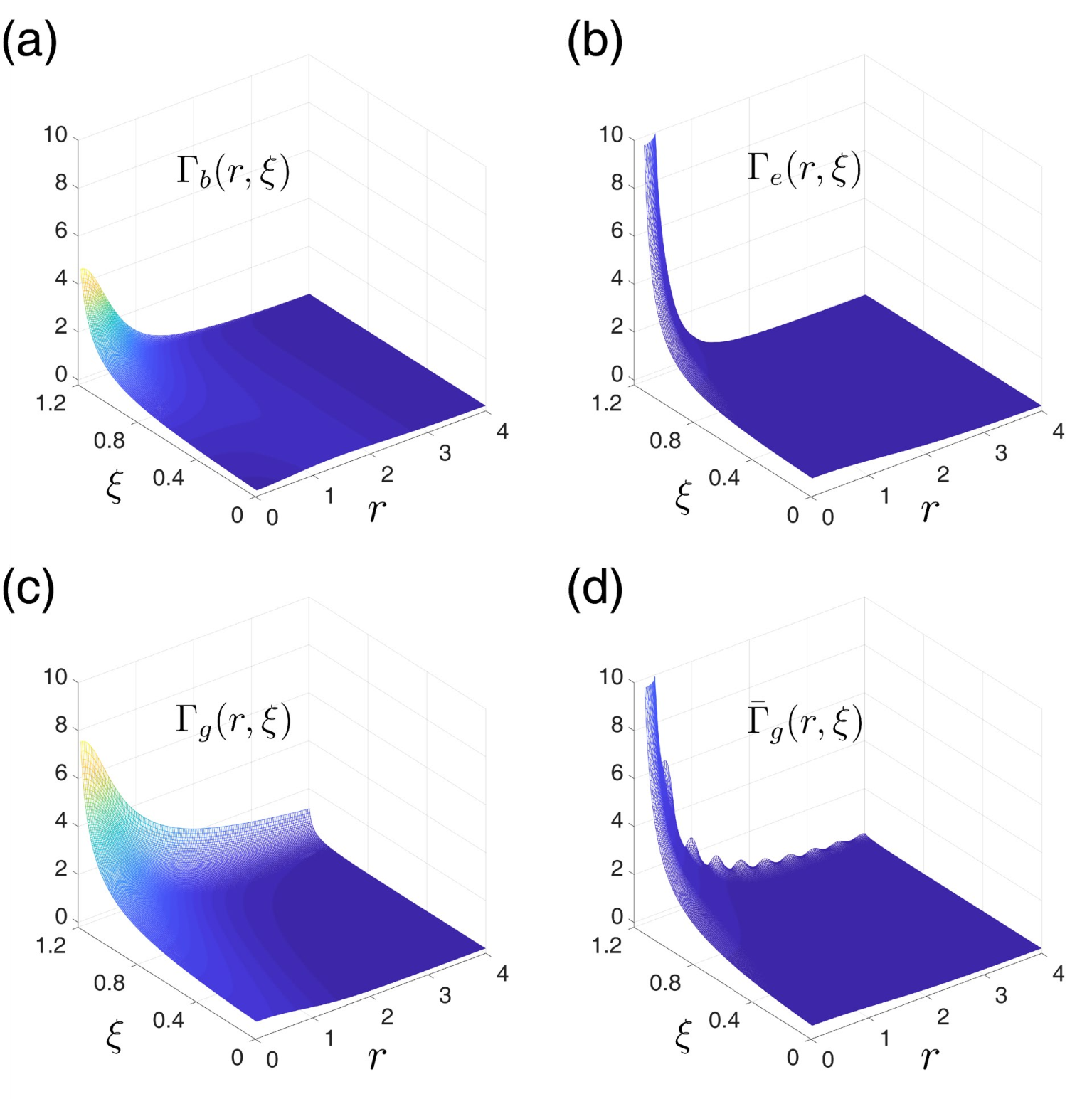
We solved Eqs. (72,73,74,75) numerically, with Γμ​(r)\Gamma_{\mu}(r) (μ=b,d,e,g\mu=b,d,e,g) and Γ¯g​(r)\overline{\Gamma}_{g}(r) at the initial RG scale (ξ=0)(\xi=0) being given by Eqs. (79,80,81, 82,83,84). By doing so, we numerically observed that in the two-dimensional AA-BB space, either a set of Γb​(r,ξ)=Γd​(r,ξ)\Gamma_{b}(r,\xi)=\Gamma_{d}(r,\xi) and Γg​(r,ξ)\Gamma_{g}(r,\xi) or a set of Γe​(r,ξ)\Gamma_{e}(r,\xi) and Γ¯g​(r,ξ)\overline{\Gamma}_{g}(r,\xi) show divergences at certain values of rr and ξ\xi (see the next section). The divergence indicates a certain type of pairing instabilities in the ground state. To identify the favored pairings and natures of resulting symmetry-broken phases, we rewrite the interaction potentials in Eq. (56) in the same basis of the Landau gauge. For example, we put e−e_{-} and h+h_{+} as well as e+e_{+} and h−h_{-} in the basis of the xx-gauge eigenstates by using Eqs. (15,16). This leads to

S1=\displaystyle S_{1}= ∫1,2,3∫dk1dk¯1dk¯2Φb(k¯2−k¯1,k1−k¯2){e+†(k1,1)e−†(k¯1,2)e−(k¯2,3)e+(k1+k¯1−k¯2,1+2−3)\displaystyle\int_{1,2,3}\int dk_{1}d\overline{k}_{1}d\overline{k}_{2}\!\ \Phi_{b}(\overline{k}_{2}-\overline{k}_{1},k_{1}-\overline{k}_{2})\!\ \!\ \Big\{\!\ e^{\dagger}_{+}(k_{1},1)e^{\dagger}_{-}(\overline{k}_{1},2)e_{-}(\overline{k}_{2},3)e_{+}(k_{1}+\overline{k}_{1}-\overline{k}_{2},1+2-3)
+h−†(k1,1)h+†(k¯1,2)h+(k¯2,3)h−(k1+k¯1−k¯2,1+2−3)}\displaystyle\hskip 93.89418pt+\!\ h^{\dagger}_{-}(k_{1},1)h^{\dagger}_{+}(\overline{k}_{1},2)h_{+}(\overline{k}_{2},3)h_{-}(k_{1}+\overline{k}_{1}-\overline{k}_{2},1+2-3)\Big\}
+∫1,2,3∫dk1dk¯1dk¯2Φe(k¯2−k¯1,k1−k¯2){e+†(k1,1)h+†(k¯1,2)h+(k¯2,3)e+(k1+k¯1−k¯2,1+2−3)\displaystyle\!\ +\int_{1,2,3}\int dk_{1}d\overline{k}_{1}d\overline{k}_{2}\!\ \Phi_{e}(\overline{k}_{2}-\overline{k}_{1},k_{1}-\overline{k}_{2})\!\ \Big\{\!\ e^{\dagger}_{+}(k_{1},1)h^{\dagger}_{+}(\overline{k}_{1},2)h_{+}(\overline{k}_{2},3)e_{+}(k_{1}+\overline{k}_{1}-\overline{k}_{2},1+2-3)
+h−†(k1,1)e−†(k¯1,2)e−(k¯2,3)h−(k1+k¯1−k¯2,1+2−3)}\displaystyle\hskip 93.89418pt+\!\ h^{\dagger}_{-}(k_{1},1)e^{\dagger}_{-}(\overline{k}_{1},2)e_{-}(\overline{k}_{2},3)h_{-}(k_{1}+\overline{k}_{1}-\overline{k}_{2},1+2-3)\Big\}
+∫1,2,3∫dk1dk2dk¯2Φg(k1−k¯2,k2−k¯2)e+†(k1,1)h−†(k2,2)h+(k¯2,3)e−(k1+k2−k¯2,1+2−3)+h.c.,\displaystyle+\int_{1,2,3}\int dk_{1}dk_{2}d\overline{k}_{2}\!\ \Phi_{g}(k_{1}-\overline{k}_{2},k_{2}-\overline{k}_{2})\!\ e^{\dagger}_{+}(k_{1},1)h^{\dagger}_{-}(k_{2},2)h_{+}(\overline{k}_{2},3)e_{-}(k_{1}+k_{2}-\overline{k}_{2},1+2-3)+{\rm h.c.}, (85)

where k1k_{1}, k¯1\overline{k}_{1}, k2k_{2} and k¯2\overline{k}_{2} are the momentum along the yy-direction. Note that due to the translational symmetry along the yy direction in the xx-gauge, all the interaction potentials preserve a center of mass in the momentum. From Eqs. (66,68,69), one can readily see that Φb​(k,k′)\Phi_{b}(k,k^{\prime}), Φe​(k,k′)\Phi_{e}(k,k^{\prime}) and Φg​(k,k′)\Phi_{g}(k,k^{\prime}) in Eq. (85) are given by Γb​(r)=Γd​(r)\Gamma_{b}(r)=\Gamma_{d}(r), Γe​(r)\Gamma_{e}(r), Γg​(r)\Gamma_{g}(r) and Γ¯g​(r)\overline{\Gamma}_{g}(r) as follows,

Φb​(k,k′)\displaystyle\Phi_{b}(k,k^{\prime}) ≡∫d​rx2​π​ei​k​rx​Γb​(rx2+k′2),\displaystyle\equiv\int\frac{dr_{x}}{2\pi}e^{ikr_{x}}\Gamma_{b}\Big(\sqrt{r^{2}_{x}+{k^{\prime}}^{2}}\Big), (86)
Φe​(k,k′)\displaystyle\Phi_{e}(k,k^{\prime}) ≡∫d​rx2​π​ei​k​rx​Γe​(rx2+k′2),\displaystyle\equiv\int\frac{dr_{x}}{2\pi}e^{ikr_{x}}\Gamma_{e}\Big(\sqrt{r^{2}_{x}+{k^{\prime}}^{2}}\Big), (87)
Φg​(k,k′)\displaystyle\Phi_{g}(k,k^{\prime}) ≡∫d​rx2​π​ei​k​rx​Γg​(rx2+k′2),\displaystyle\equiv\int\frac{dr_{x}}{2\pi}e^{ikr_{x}}\Gamma_{g}\Big(\sqrt{r^{2}_{x}+{k^{\prime}}^{2}}\Big), (88)
≡∫d​ry2​π​ei​k′​ry​Γ¯g​(k2+ry2).\displaystyle\equiv\int\frac{dr_{y}}{2\pi}e^{ik^{\prime}r_{y}}\overline{\Gamma}_{g}\Big(\sqrt{k^{2}+r^{2}_{y}}\Big). (89)

One could also rewrite e+e_{+} and h−h_{-} as well as e−e_{-} and h+h_{+} in the basis of the yy-gauge eigenstates. Of course, this leads to the same conclusions as we will reach in the xx-gauge eigenstates (see the following two sections).

V Ground-state phase diagram in the presence of repulsive Coulomb interaction

The parquet RG equations have a dual structure; Γb​(r)=Γd​(r)\Gamma_{b}(r)=\Gamma_{d}(r) and Γg​(r)\Gamma_{g}(r) couple with each other exactly in the same way as Γe​(r)\Gamma_{e}(r) and Γ¯g​(r)\overline{\Gamma}_{g}(r) do, and Γg​(r)\Gamma_{g}(r) and Γ¯g​(r)\overline{\Gamma}_{g}(r) are Fourier transforms of the other [Eqs. (77,78)]. In the case of the repulsive interaction, this dual structure in the RG equations leads to a ground-state competition between the excitonic insulator phase brazovskii72 and Ising-type spin density wave phase (Fig. 1). The numerical solution of the RG equations shows that in the two-dimensional AA-BB parameter space, either a set of Γe​(r)\Gamma_{e}(r) and Γ¯g​(r)\overline{\Gamma}_{g}(r) or a set of Γb​(r)\Gamma_{b}(r) and Γg​(r)\Gamma_{g}(r) diverge at a certain critical RG scale, ξ=ξc\xi=\xi_{c}.

Refer to caption
Figure 7: Numerical solution of the parquet RG equations, Eqs. (72,73,74,75), with the initial interaction forms given by Eqs. (79,80,81,82) in the strong screening regime (log10⁡A=0\log_{10}A=0 and log10⁡B=0\log_{10}B=0). The solution tells how the interaction potentials of rr, Γb​(r,ξ)=Γd​(r,ξ)\Gamma_{b}(r,\xi)=\Gamma_{d}(r,\xi), Γe​(r,ξ)\Gamma_{e}(r,\xi), Γg​(r,ξ)\Gamma_{g}(r,\xi) and Γ¯g​(r,ξ)\overline{\Gamma}_{g}(r,\xi), grow as a function of the RG scale ξ\xi. Γe​(r,ξ)\Gamma_{e}(r,\xi) and Γ¯g​(r,ξ)\overline{\Gamma}_{g}(r,\xi) help each other and show the diverge at r=0r=0 around ξ=1.2\xi=1.2.

V.1 strong screening region

To understand the phase diagram qualitatively, let us keep only those terms in the parquet RG equations that couple the functions locally in the radial coordinate rr; brazovskii72; yakovenko93; tsai02a; alicea09

d​Γb/d​(r,ξ)d​ξ\displaystyle\frac{d\Gamma_{b/d}(r,\xi)}{d\xi} =Γb/d2​(r,ξ)+Γg2​(r,ξ),\displaystyle=\Gamma^{2}_{b/d}(r,\xi)+\Gamma^{2}_{g}(r,\xi), (90)
d​Γg​(r,ξ)d​ξ\displaystyle\frac{d\Gamma_{g}(r,\xi)}{d\xi} =Γg2​(r,ξ)​(Γb​(r,ξ)+Γd​(r,ξ)),\displaystyle=\Gamma^{2}_{g}(r,\xi)\big(\Gamma_{b}(r,\xi)+\Gamma_{d}(r,\xi)\big), (91)

and

d​Γe​(r,ξ)d​ξ\displaystyle\frac{d\Gamma_{e}(r,\xi)}{d\xi} =Γe2​(r,ξ)+Γ¯e2​(r,ξ),\displaystyle=\Gamma^{2}_{e}(r,\xi)+\overline{\Gamma}^{2}_{e}(r,\xi), (92)
d​Γ¯g​(r,ξ)d​ξ\displaystyle\frac{d\overline{\Gamma}_{g}(r,\xi)}{d\xi} =2​Γ¯g2​(r,ξ)​Γe​(r,ξ).\displaystyle=2\overline{\Gamma}^{2}_{g}(r,\xi)\Gamma_{e}(r,\xi). (93)

When the RG scale is near (but below) the critical RG scale, ξ≲ξc\xi\lesssim\xi_{c}, the local terms become leading order than those terms neglected, and the approximation and solutions below are justified. Without the constraint between Γg​(r)\Gamma_{g}(r) and Γ¯g​(r)\overline{\Gamma}_{g}(r) (Eqs. (77),(78)), the approximate RG equations can be solved and the solutions are determined only by the initial forms of the interaction potentials,

Γb/d​(r,ξ)\displaystyle\Gamma_{b/d}(r,\xi) =12​{11Γb/d​(r,0)+Γg​(r,0)−ξ+11Γb/d​(r,0)−Γg​(r,0)−ξ},\displaystyle=\frac{1}{2}\bigg\{\frac{1}{\frac{1}{\Gamma_{b/d}(r,0)+\Gamma_{g}(r,0)}-\xi}+\frac{1}{\frac{1}{\Gamma_{b/d}(r,0)-\Gamma_{g}(r,0)}-\xi}\bigg\}, (94)
Γg​(r,ξ)\displaystyle\Gamma_{g}(r,\xi) =12​{11Γb/d​(r,0)+Γg​(r,0)−ξ−11Γb/d​(r,0)−Γg​(r,0)−ξ},\displaystyle=\frac{1}{2}\bigg\{\frac{1}{\frac{1}{\Gamma_{b/d}(r,0)+\Gamma_{g}(r,0)}-\xi}-\frac{1}{\frac{1}{\Gamma_{b/d}(r,0)-\Gamma_{g}(r,0)}-\xi}\bigg\}, (95)

and

Γe​(r,ξ)\displaystyle\Gamma_{e}(r,\xi) =12​{11Γe​(r,0)+Γ¯g​(r,0)−ξ+11Γe​(r,0)−Γ¯g​(r,0)−ξ},\displaystyle=\frac{1}{2}\bigg\{\frac{1}{\frac{1}{\Gamma_{e}(r,0)+\overline{\Gamma}_{g}(r,0)}-\xi}+\frac{1}{\frac{1}{\Gamma_{e}(r,0)-\overline{\Gamma}_{g}(r,0)}-\xi}\bigg\}, (96)
Γ¯g​(r,ξ)\displaystyle\overline{\Gamma}_{g}(r,\xi) =12​{11Γe​(r,0)+Γ¯g​(r,0)−ξ−11Γe​(r,0)−Γ¯g​(r,0)−ξ}.\displaystyle=\frac{1}{2}\bigg\{\frac{1}{\frac{1}{\Gamma_{e}(r,0)+\overline{\Gamma}_{g}(r,0)}-\xi}-\frac{1}{\frac{1}{\Gamma_{e}(r,0)-\overline{\Gamma}_{g}(r,0)}-\xi}\bigg\}. (97)

With Eqs. (79,80,81,82,83,84) at the initial RG scale (ξ=0\xi=0), Γe​(r,0)+Γ¯g​(r,0)\Gamma_{e}(r,0)+\overline{\Gamma}_{g}(r,0) takes the largest positive value at r=0r=0 among the other three at any rr,

Γe​(r=0,0)+Γ¯g​(r=0,0)\displaystyle\Gamma_{e}(r=0,0)+\overline{\Gamma}_{g}(r=0,0)
≥Γe​(r,0)±Γ¯g​(r,0),Γb​(r,0)±Γg​(r,0).\displaystyle\geq\Gamma_{e}(r,0)\pm\overline{\Gamma}_{g}(r,0),\Gamma_{b}(r,0)\pm\Gamma_{g}(r,0).

Thus, the approximate solution dictates that positive Γe​(r,ξ)\Gamma_{e}(r,\xi) and positive Γ¯g​(r,ξ)\overline{\Gamma}_{g}(r,\xi) diverge at r=0r=0 simultaneously on the renormalization as brazovskii72,

Γe(r,ξc)=Γ¯g(r,ξc)=A′r2+⋯(A′>0).\displaystyle\Gamma_{e}(r,\xi_{c})=\overline{\Gamma}_{g}(r,\xi_{c})=\frac{A^{\prime}}{r^{2}}+\cdots\!\ (A^{\prime}>0). (98)

Fig. 7 demonstrates how the four interaction potentials, Γb​(r,ξ)=Γd​(r,ξ)\Gamma_{b}(r,\xi)=\Gamma_{d}(r,\xi), Γe​(r,ξ)\Gamma_{e}(r,\xi), Γg​(r,ξ)\Gamma_{g}(r,\xi) and Γ¯g​(r,ξ)\overline{\Gamma}_{g}(r,\xi), change their forms under the parquet RG equations, Eqs.(72,73,74,75), in the strong screening regime.

When Γe​(r=0)\Gamma_{e}(r=0) and Γ¯g​(r=0)\overline{\Gamma}_{g}(r=0) dominate over the others, an excitonic pairing is formed between electron and hole bands at the same Fermi point and at the same spatial coordinate within the x​yxy plane,

⟨e+†​(ky)​h+​(ky)⟩=⟨e−†​(ky)​h−​(ky)⟩≠0,\displaystyle\langle e^{\dagger}_{+}(k_{y})h_{+}(k_{y})\rangle=\langle e^{\dagger}_{-}(k_{y})h_{-}(k_{y})\rangle\neq 0, (99)
⟨e+†​(qx)​h+​(qx)⟩=⟨e−†​(qx)​h−​(qx)⟩≠0.\displaystyle\langle e^{\dagger}_{+}(q_{x})h_{+}(q_{x})\rangle=\langle e^{\dagger}_{-}(q_{x})h_{-}(q_{x})\rangle\neq 0. (100)

Namely, the asymptotic forms of Γe​(r,ξc)\Gamma_{e}(r,\xi_{c}) and Γ¯g​(r,ξc)\overline{\Gamma}_{g}(r,\xi_{c}) make the following scattering channels in Eq. (85) to be dominant among the others,

Φe(k¯2−k¯1,k1−k¯2=0)→+∞,\displaystyle\Phi_{e}(\overline{k}_{2}-\overline{k}_{1},k_{1}-\overline{k}_{2}=0)\rightarrow+\infty, (101)
Φg(k1−k¯2=0,k2−k¯2)→+∞,\displaystyle\Phi_{g}(k_{1}-\overline{k}_{2}=0,k_{2}-\overline{k}_{2})\rightarrow+\infty, (102)

for arbitrary k¯2−k¯1\overline{k}_{2}-\overline{k}_{1} (Eq. (101)) and arbitrary k2−k¯2k_{2}-\overline{k}_{2} (Eq. (102)) respectively. These scatterings favor electron-hole pairings at the same Fermi points and at the same two-dimensional space coordinates within the x​yxy plane;

S1=−\displaystyle S_{1}=- ∫1,2,3∫k1−k¯2=0d​k1​d​k¯1​d​k¯2​Φe​(k¯2−k¯1,k1−k¯2)\displaystyle\int_{1,2,3}\int_{k_{1}-\overline{k}_{2}=0}dk_{1}d\overline{k}_{1}d\overline{k}_{2}\!\ \Phi_{e}(\overline{k}_{2}-\overline{k}_{1},k_{1}-\overline{k}_{2})
{⟨e+†(k¯2,1)h+(k¯2,3)⟩⟨h+†(k¯1,2)e+(k¯1,1+2−3)⟩\displaystyle\hskip-34.14322pt\Big\{\!\ \big\langle e^{\dagger}_{+}(\overline{k}_{2},1)h_{+}(\overline{k}_{2},3)\big\rangle\big\langle h^{\dagger}_{+}(\overline{k}_{1},2)e_{+}(\overline{k}_{1},1+2-3)\big\rangle
+⟨h−†(k¯2,1)e−(k¯2,3)⟩⟨e−†(k¯1,2)h−(k¯1,1+2−3)⟩}\displaystyle\hskip-28.45274pt+\big\langle h^{\dagger}_{-}(\overline{k}_{2},1)e_{-}(\overline{k}_{2},3)\big\rangle\big\langle e^{\dagger}_{-}(\overline{k}_{1},2)h_{-}(\overline{k}_{1},1+2-3)\big\rangle\Big\}
−∫1,2,3∫k1−k¯2=0dk1dk¯1dk¯2Φg(k¯1−k¯2,k2−k¯2)\displaystyle-\int_{1,2,3}\int_{k_{1}-\overline{k}_{2}=0}dk_{1}d\overline{k}_{1}d\overline{k}_{2}\!\ \Phi_{g}(\overline{k}_{1}-\overline{k}_{2},k_{2}-\overline{k}_{2})
{⟨e+†(k¯2,1)h+(k¯2,3)⟩⟨h−†(k2,2)e−(k2,1+2−3)⟩\displaystyle\hskip-34.14322pt\Big\{\!\ \big\langle e^{\dagger}_{+}(\overline{k}_{2},1)h_{+}(\overline{k}_{2},3)\big\rangle\big\langle h^{\dagger}_{-}(k_{2},2)e_{-}(k_{2},1+2-3)\big\rangle
+c.c.}+⋯.\displaystyle\hskip 113.81102pt+{\rm c.c.}\Big\}+\cdots. (103)

Note that the relative U(1) phase between the excitonic pairing field at the right Fermi point and that at the left Fermi point is locked to be zero by the positively large Φg(k1−k¯2=0,k2−k¯2)\Phi_{g}(k_{1}-\overline{k}_{2}=0,k_{2}-\overline{k}_{2}).

The excitonic pairing between the electron band with ↑\uparrow spin and the hole band with ↓\downarrow spin results in a ferro-type order of an X​YXY component of the spin-1 moment;

⟨Ψe,↑†​(𝒓)​Ψh,↓​(𝒓)⟩≡X⁡(𝒓)+i​Y​(𝒓)∝ei​θ.\displaystyle\langle\Psi^{\dagger}_{e,\uparrow}({\bm{r}})\Psi_{h,\downarrow}({\bm{r}})\rangle\equiv X({\bm{r}})+iY({\bm{r}})\propto e^{i\theta}. (104)

The ferro-type order breaks the U(1) spin rotational symmetry around the magnetic field. However, detailed microscopic magnetism of the excitonic phase depends on atomic orbitals (localized Wannier orbitals) that form the electron band and the hole band.

Figure 8: Schematic picture of Ising-type spin density wave. The ↑\uparrow and ↓\downarrow arrows are spins along the field. The horizontal axis is along the field direction.

V.2 weak screening region

When the screening length is longer than the magnetic length [A≥3A\geq 3 for 2​kF​l≃12k_{F}l\simeq 1], the numerical solution shows that Γb​(r)\Gamma_{b}(r) and Γg​(r)\Gamma_{g}(r) diverges at r=0r=0 as;

Γb(r,ξc)=Γg(r,ξc)=A′r2+⋯(A′>0).\displaystyle\Gamma_{b}(r,\xi_{c})=\Gamma_{g}(r,\xi_{c})=\frac{A^{\prime}}{r^{2}}+\cdots\!\ \!\ (A^{\prime}>0).

The divergence identifies the relevant scattering channels in Eq. (85) as,

Φb(k¯2−k¯1,k1−k¯2=0)→+∞,\displaystyle\Phi_{b}(\overline{k}_{2}-\overline{k}_{1},k_{1}-\overline{k}_{2}=0)\rightarrow+\infty,

for any k¯2−k¯1\overline{k}_{2}-\overline{k}_{1}, and

Φg(k1−k¯2,k2−k¯2=0)→+∞,\displaystyle\Phi_{g}(k_{1}-\overline{k}_{2},k_{2}-\overline{k}_{2}=0)\rightarrow+\infty,

for any k1−k¯2k_{1}-\overline{k}_{2}. These scattering channels cause an instability to a charge density wave of the electron band and that of the hole band,

⟨e+†​(k)​e−​(k)⟩=ei​π​⟨h+†​(k)​h−​(k)⟩.\displaystyle\langle e^{\dagger}_{+}(k)e_{-}(k)\rangle=e^{i\pi}\langle h^{\dagger}_{+}(k)h_{-}(k)\rangle. (105)

Both density waves share the same spatial pitch (2​π/2​kF2\pi/2k_{F}) along the field direction. The relative U(1) phase between the electron-band density wave and hole-hand density wave is locked to be π\pi by the positively large Φg(k1−k¯2,k2−k¯2=0)\Phi_{g}(k_{1}-\overline{k}_{2},k_{2}-\overline{k}_{2}=0). Due to the π\pi phase shift, the ground state in the weak screening region is accompanied by Ising-type spin density wave that preserves the U(1) spin rotational symmetry around the magnetic field (Fig. 8).

VI Ground-state phase diagram in the presence of effective attractive interaction

In the previous section, we have studied how the repulsive Coulomb interaction leads to the low-temperature instability in the semimetal under high magnetic field. As the complimentary aspect, we consider in this section an effect of another relevant many-body interaction; electron-(acoustic) phonon interaction. We employ an argument based on an equivalence between an electron-phonon coupled system and a system with an electron-electron interaction, and adopt the following effective attractive electron-electron interaction;

Heff\displaystyle H_{\rm eff} =12​∫d3​𝒓​d3​𝒓′​ρ​(𝒓)​ρ​(𝒓′)​Veff​(𝒓−𝒓′),\displaystyle=\frac{1}{2}\int d^{3}{\bm{r}}d^{3}{\bm{r}}^{\prime}\rho({\bm{r}})\rho({\bm{r}}^{\prime})V_{\rm eff}({\bm{r}}-{\bm{r}}^{\prime}), (106)
Veff​(𝒓)\displaystyle V_{\rm eff}({\bm{r}}) =∫d3​𝒒(2​π)3​Veff​(𝒒)​ei​𝒒​𝒓,\displaystyle=\int\frac{d^{3}{\bm{q}}}{(2\pi)^{3}}V_{\rm eff}({\bm{q}})\!\ e^{i{\bm{q}}{\bm{r}}}, (107)
Veff​(𝒒)\displaystyle V_{\rm eff}({\bm{q}}) ≡−Ueff2​(𝒒),\displaystyle\equiv-U^{2}_{\rm eff}({\bm{q}}), (108)
Ueff​(𝒒)\displaystyle U_{\rm eff}({\bm{q}}) ≡(ρ0M)12​4​π​Z​e2​l2ε​c​1(qz2+q⟂2)​l2+A−1​e−12​q⟂2​l2.\displaystyle\equiv\Big(\frac{\rho_{0}}{M}\Big)^{\frac{1}{2}}\frac{4\pi Ze^{2}l^{2}}{\varepsilon c}\frac{1}{(q^{2}_{z}+q^{2}_{\perp})l^{2}+A^{-1}e^{-\frac{1}{2}q^{2}_{\perp}l^{2}}}. (109)

Here Ueff​(𝒒)U_{\rm eff}({\bm{q}}) is the Fourier transform of a screened Coulomb potential between electron and (longitudinal acoustic) phonon. ZZ and cc are an electron valence of positively charged nucleus ion and a sound velocity of the acoustic phonon respectively, ρ0\rho_{0} and MM is the density of the charged nuclei, and a mass of the charged nucleus ion. Within the random phase approximation, (the square of) the screening length ‘AA’ in Ueff​(𝒒)U_{\rm eff}({\bm{q}}) was calculated in the previous section [Eq. (53,54)]. Here we consider the case with A=A′A=A^{\prime} for simplicity.

Using Eqs. (106,107,108,109) as the effective electron-electron interaction, we study low-temperature instabilities in semimetal under high magnetic field in the presence of the electron-phonon coupling. To this end, we solve numerically the same parquet RG equations as in the previous section, while we use the following set as the interaction forms at the initial RG scale (ξ=0\xi=0);

Γb/d​(r)≡−2​π​{∫0∞r′​d​r′​J0​(r​r′)​I¯0′​(r′)−I¯2​kF′​(r)},\displaystyle\Gamma_{b/d}(r)\equiv-2\pi\Big\{\int^{\infty}_{0}r^{\prime}dr^{\prime}J_{0}(rr^{\prime})\overline{I}^{\prime}_{0}(r^{\prime})-\overline{I}^{\prime}_{2k_{F}}(r)\Big\}, (110)
Γe(r)≡−2π∫0∞r′dr′J0(rr′)I¯0′(r′),\displaystyle\Gamma_{e}(r)\equiv-2\pi\int^{\infty}_{0}r^{\prime}dr^{\prime}J_{0}(rr^{\prime})\overline{I}^{\prime}_{0}(r^{\prime}), (111)
Γg​(r)≡−2​π​I¯2​kF′​(r),\displaystyle\Gamma_{g}(r)\equiv-2\pi\overline{I}^{\prime}_{2k_{F}}(r), (112)
Γ¯g(r)≡−2π∫0∞r′dr′J0(rr′)I¯2​kF′(r′),\displaystyle\overline{\Gamma}_{g}(r)\equiv-2\pi\int^{\infty}_{0}r^{\prime}dr^{\prime}J_{0}(rr^{\prime})\overline{I}^{\prime}_{2k_{F}}(r^{\prime}), (113)

with

I¯0′​(r)\displaystyle\overline{I}^{\prime}_{0}(r) ≡(4​π​Z​e2​l2ε​c)2​ρ0M​e12​r2(r2​e12​r2+A−1)2,\displaystyle\equiv\Big(\frac{4\pi Ze^{2}l^{2}}{\varepsilon c}\Big)^{2}\frac{\rho_{0}}{M}\frac{e^{\frac{1}{2}r^{2}}}{(r^{2}e^{\frac{1}{2}r^{2}}+A^{-1})^{2}}, (114)
I¯2​kF′​(r)\displaystyle\overline{I}^{\prime}_{2k_{F}}(r) ≡(4​π​Z​e2​l2ε​c)2​ρ0M​e12​r2((r2+B)​e12​r2+A−1)2.\displaystyle\equiv\Big(\frac{4\pi Ze^{2}l^{2}}{\varepsilon c}\Big)^{2}\frac{\rho_{0}}{M}\frac{e^{\frac{1}{2}r^{2}}}{\big((r^{2}+B)e^{\frac{1}{2}r^{2}}+A^{-1}\big)^{2}}. (115)

Again, the overall factor of I¯0′​(r)\overline{I}^{\prime}_{0}(r) and I¯2​kF′​(r)\overline{I}^{\prime}_{2k_{F}}(r) does not play any role in a determination of the phase diagram within the one-loop RG analyses. Only the two dimensionless parameters AA and BB play the crucial role.

VI.1 intermediate screening region

Fig. 2 is a phase diagram obtained by the numerical solutions. In an intermediate screening region (A≃10−1A\simeq 10^{-1}), the ground state shows an instability toward a charge Wigner crystal phase, where Γb​(r)\Gamma_{b}(r) and Γg​(r)\Gamma_{g}(r) diverges at nonzero rr (r=rc≠0r=r_{c}\neq 0) at a certain critical RG scale (ξ=ξc\xi=\xi_{c}) as,

Γb(r,ξc)=−Γg(r,ξc)=A′′|r−rc|2+⋯(A′′>0).\displaystyle\Gamma_{b}(r,\xi_{c})=-\Gamma_{g}(r,\xi_{c})=\frac{A^{\prime\prime}}{|r-r_{c}|^{2}}+\cdots\!\ \!\ (A^{\prime\prime}>0). (116)

Substituting this into Eqs. (86,88), one can see that dominant scattering channels in Eq. (85) take the following asymptotic forms,

Φb(k¯2−k¯1,k1−k¯2=rccosθ)\displaystyle\Phi_{b}(\overline{k}_{2}-\overline{k}_{1},k_{1}-\overline{k}_{2}=r_{c}\cos\theta)
→cos⁡((k¯2−k¯1)​rc​sin⁡θ)×(+∞),\displaystyle\hskip 56.9055pt\rightarrow\cos\big((\overline{k}_{2}-\overline{k}_{1})r_{c}\sin\theta\big)\times(+\infty), (117)
Φg(k1−k¯2,k¯2−k2=rccosθ)\displaystyle\Phi_{g}(k_{1}-\overline{k}_{2},\overline{k}_{2}-k_{2}=r_{c}\cos\theta)
→cos⁡((k1−k¯2)​rc​sin⁡θ)×(−∞),\displaystyle\hskip 56.9055pt\rightarrow\cos\big((k_{1}-\overline{k}_{2})r_{c}\sin\theta\big)\times(-\infty), (118)

for any θ∈[0,π)\theta\in[0,\pi), and for any k¯2−k¯1\overline{k}_{2}-\overline{k}_{1} (Eq. (117)) and any k1−k¯2k_{1}-\overline{k}_{2} (Eq. (118)), respectively. The scattering channels induce 2​kF2k_{F} density-wave pairings within the electron band and hole hand. The induced density-wave pairings generally connect different two-dimensional coordinates within the x​yxy plane,

S1≡\displaystyle S_{1}\equiv ∫0πd​θ​rc​sin⁡θ​S1​(θ)+⋯,\displaystyle\int^{\pi}_{0}d\theta\!\ r_{c}\sin\theta\!\ S_{1}(\theta)+\cdots,
S1(θ)=−\displaystyle S_{1}(\theta)=- ∫1,2,3∫dk¯1dk¯2Φb(k¯2−k¯1,rccosθ){⟨e+†(k¯2+rccosθ,1)e−(k¯2,3)⟩⟨e−†(k¯1,2)e+(k¯1+rccosθ,⋯)⟩\displaystyle\int_{1,2,3}\int d\overline{k}_{1}d\overline{k}_{2}\!\ \Phi_{b}(\overline{k}_{2}-\overline{k}_{1},r_{c}\cos\theta)\Big\{\!\ \big\langle e^{\dagger}_{+}(\overline{k}_{2}+r_{c}\cos\theta,1)e_{-}(\overline{k}_{2},3)\big\rangle\big\langle e^{\dagger}_{-}(\overline{k}_{1},2)e_{+}(\overline{k}_{1}+r_{c}\cos\theta,\cdots)\big\rangle
+⟨h−†(k¯2−rccosθ,1)h+(k¯2,3)⟩⟨h+†(k¯1,2)h−(k¯1−rccosθ,⋯)⟩}\displaystyle\hskip 14.22636pt+\big\langle h^{\dagger}_{-}(\overline{k}_{2}-r_{c}\cos\theta,1)h_{+}(\overline{k}_{2},3)\big\rangle\big\langle h^{\dagger}_{+}(\overline{k}_{1},2)h_{-}(\overline{k}_{1}-r_{c}\cos\theta,\cdots)\big\rangle\Big\}
+∫1,2,3∫dk1dk¯2Φg(k1−k¯2,rccosθ)⟨e+†(k1,1)e−(k1−rccosθ,⋯)⟩⟨h−†(k¯2−rccosθ,2)h+(k¯2,3)⟩+c.c..\displaystyle\hskip-42.67912pt+\int_{1,2,3}\int dk_{1}d\overline{k}_{2}\!\ \Phi_{g}(k_{1}-\overline{k}_{2},r_{c}\cos\theta)\!\ \big\langle e^{\dagger}_{+}(k_{1},1)e_{-}(k_{1}-r_{c}\cos\theta,\cdots)\big\rangle\big\langle h^{\dagger}_{-}(\overline{k}_{2}-r_{c}\cos\theta,2)h_{+}(\overline{k}_{2},3)\big\rangle+{\rm c.c.}. (119)

Due to the coordinate-dependent (kk-dependent) cosine functions in Eqs. (117,118), the action S1​(θ)S_{1}(\theta) is fully minimized by the pairing fields that have coordinate-dependent phases,

⟨e+†​(k)​e−​(k−rc​cos⁡θ)⟩\displaystyle\langle e^{\dagger}_{+}(k)e_{-}(k-r_{c}\cos\theta)\rangle =⟨h+†​(k)​h−​(k−rc​cos⁡θ)⟩\displaystyle=\langle h^{\dagger}_{+}(k)h_{-}(k-r_{c}\cos\theta)\rangle
=B​e−i​λ∓i​k​rc​sin⁡θ.\displaystyle=Be^{-i\lambda\mp ikr_{c}\sin\theta}. (120)

Such pairings lead to the density waves in the electron and hole bands, that break the translational symmetries within the x​yxy plane,

⟨Ψe,↑†​(𝒓)​Ψe,↑​(𝒓)⟩=⟨Ψh,↓†​(𝒓)​Ψh,↓​(𝒓)⟩\displaystyle\langle\Psi^{\dagger}_{e,\uparrow}({\bm{r}})\Psi_{e,\uparrow}({\bm{r}})\rangle=\langle\Psi^{\dagger}_{h,\downarrow}({\bm{r}})\Psi_{h,\downarrow}({\bm{r}})\rangle
=B′​cos⁡(2​kF​z+rc​(y​cos⁡θ±x​sin⁡θ)+λ′).\displaystyle=B^{\prime}\cos\big(2k_{F}z+r_{c}(y\!\ \cos\theta\pm x\!\ \sin\theta)+\lambda^{\prime}\big).

The density wave of the electron band with ↑\uparrow spin and the density wave of the hole band with the ↓\downarrow spin have the same phase; the superpose of these two is nothing but the charge density wave without any spin texture. The spatial pitches within the x​yxy plane and along the field direction is 2​π​l/rc2\pi l/r_{c} and 2​π/(2​kF)2\pi/(2k_{F}) respectively.

The ‘propagation’ direction of the density wave within the x​yxy plane is specified by θ\theta, that can take any value in [0,π)[0,\pi) according to Eqs. (117,118,119). The ground state is generally a superposition of the density waves with different propagation directions within the x​yxy plane. One of the most plausible superposition is a symmetric superposition,

⟨Ψe,↑†​(𝒓)​Ψe,↑​(𝒓)⟩=⟨Ψh,↓†​(𝒓)​Ψh,↓​(𝒓)⟩\displaystyle\langle\Psi^{\dagger}_{e,\uparrow}({\bm{r}})\Psi_{e,\uparrow}({\bm{r}})\rangle=\langle\Psi^{\dagger}_{h,\downarrow}({\bm{r}})\Psi_{h,\downarrow}({\bm{r}})\rangle
∝∑j=1,2,3cos⁡(2​kF​z+rc​𝒏j⋅𝒓⟂+θ)+const,\displaystyle\ \ \ \propto\sum_{j=1,2,3}\cos\big(2k_{F}z+r_{c}{\bm{n}}_{j}\cdot{\bm{r}}_{\perp}+\theta\big)+{\rm const}, (121)

with 𝒓⟂=(x,y){\bm{r}}_{\perp}=(x,y), 𝒏1=(1,0){\bm{n}}_{1}=(1,0), 𝒏2=(−12,32){\bm{n}}_{2}=(-\frac{1}{2},\frac{\sqrt{3}}{2}), and 𝒏3=(−12,−32){\bm{n}}_{3}=(-\frac{1}{2},-\frac{\sqrt{3}}{2}) [or its O(2) rotation within the x​yxy plane]. This leads to a triangle lattice of the charge density within the x​yxy plane (charge Wigner crystal; Fig. 9(a)).

VI.2 strong screening region

In a strong screening region (A<10−2A<10^{-2}), the ground state exhibits an instability to an excitonic phase, where Γe​(r)\Gamma_{e}(r) and Γ¯g​(r)\overline{\Gamma}_{g}(r) diverge at nonzero rr (r=rc≠0r=r_{c}\neq 0) at the critical RG scale (ξ=ξc\xi=\xi_{c}) as;

Γe​(r,ξc)=Γ¯g​(r,ξc)=A′′|r−rc|2+⋯,(A′′>0).\displaystyle\Gamma_{e}(r,\xi_{c})=\overline{\Gamma}_{g}(r,\xi_{c})=\frac{A^{\prime\prime}}{|r-r_{c}|^{2}}+\cdots,\!\ \!\ (A^{\prime\prime}>0). (122)

The divergence gives rise to the following forms of the dominant scattering channels in Eq. (85),

Φe(k¯2−k¯1,k1−k¯2=rccosθ)\displaystyle\Phi_{e}(\overline{k}_{2}-\overline{k}_{1},k_{1}-\overline{k}_{2}=r_{c}\cos\theta)
→cos⁡((k¯2−k¯1)​rc​sin⁡θ)×(+∞),\displaystyle\hskip 56.9055pt\rightarrow\cos\big((\overline{k}_{2}-\overline{k}_{1})r_{c}\sin\theta\big)\times(+\infty), (123)
Φg(k1−k¯2=rccosθ,k2−k¯2)\displaystyle\Phi_{g}(k_{1}-\overline{k}_{2}=r_{c}\cos\theta,k_{2}-\overline{k}_{2})
→cos⁡((k2−k¯2)​rc​sin⁡θ)×(+∞),\displaystyle\hskip 56.9055pt\rightarrow\cos\big((k_{2}-\overline{k}_{2})r_{c}\sin\theta\big)\times(+\infty), (124)

for any θ\theta, and for any k¯2−k¯1\overline{k}_{2}-\overline{k}_{1} (Eq. (123)) and any k2−k¯2k_{2}-\overline{k}_{2} (Eq. (124)) respectively. These scattering channels mediate the excitonic pairings between different spatial coordinate within the x​yxy plane;

S1≡\displaystyle S_{1}\equiv ∫0πd​θ​rc​sin⁡θ​S1​(θ)+⋯\displaystyle\int^{\pi}_{0}d\theta\!\ r_{c}\sin\theta\!\ S_{1}(\theta)+\cdots
S1(θ)=−\displaystyle S_{1}(\theta)=- ∫1,2,3∫dk¯1dk¯2Φe(k¯2−k¯1,rccosθ){⟨e+†(k¯2+rccosθ,1)h+(k¯2,3)⟩⟨h+†(k¯1,2)e+(k¯1+rccosθ,⋯)⟩\displaystyle\int_{1,2,3}\int d\overline{k}_{1}d\overline{k}_{2}\!\ \Phi_{e}(\overline{k}_{2}-\overline{k}_{1},r_{c}\cos\theta)\Big\{\!\ \big\langle e^{\dagger}_{+}(\overline{k}_{2}+r_{c}\cos\theta,1)h_{+}(\overline{k}_{2},3)\big\rangle\big\langle h^{\dagger}_{+}(\overline{k}_{1},2)e_{+}(\overline{k}_{1}+r_{c}\cos\theta,\cdots)\big\rangle
+⟨h−†(k¯2−rccosθ,1)e−(k¯2,3)⟩⟨e−†(k¯1,2)h−(k¯1−rccosθ,⋯)⟩}\displaystyle\hskip 28.45274pt+\big\langle h^{\dagger}_{-}(\overline{k}_{2}-r_{c}\cos\theta,1)e_{-}(\overline{k}_{2},3)\big\rangle\big\langle e^{\dagger}_{-}(\overline{k}_{1},2)h_{-}(\overline{k}_{1}-r_{c}\cos\theta,\cdots)\big\rangle\Big\}
−∫1,2,3∫dk2dk¯2Φg(rccosθ,k2−k¯2)⟨e+†(k¯2+rccosθ,1)h+(k¯2,3)⟩⟨h−†(k2,2)e−(k2+rccosθ,⋯)⟩+c.c..\displaystyle\hskip-45.52458pt-\int_{1,2,3}\int dk_{2}d\overline{k}_{2}\!\ \Phi_{g}(r_{c}\cos\theta,k_{2}-\overline{k}_{2})\big\langle e^{\dagger}_{+}(\overline{k}_{2}+r_{c}\cos\theta,1)h_{+}(\overline{k}_{2},3)\big\rangle\big\langle h^{\dagger}_{-}(k_{2},2)e_{-}(k_{2}+r_{c}\cos\theta,\cdots)\big\rangle+{\rm c.c.}. (125)

Namely, the action with Eqs. (123,124) is minimized by the excitonic pairing within the same Fermi points but between different spatial coordinates within the x​yxy plane. The pairing fields thus determined have the coordinate-dependent phase factors,

⟨e+†​(k¯2+rc​cos⁡θ)​h+​(k¯2)⟩\displaystyle\langle e^{\dagger}_{+}(\overline{k}_{2}+r_{c}\cos\theta)h_{+}(\overline{k}_{2})\rangle =⟨e−†​(k¯2+rc​cos⁡θ)​h−​(k¯2)⟩\displaystyle=\langle e^{\dagger}_{-}(\overline{k}_{2}+r_{c}\cos\theta)h_{-}(\overline{k}_{2})\rangle
=C​ei​ψ±i​k¯2​rc​sin⁡θ.\displaystyle=Ce^{i\psi\pm i\overline{k}_{2}r_{c}\sin\theta}. (126)

Such excitonic pairings leads to a density wave of the X​YXY component of the spin-1 moment, that breaks the translational symmetry within the x​yxy plane;

⟨Ψe,↑†​(𝒓)​Ψh,↓​(𝒓)⟩≡X⁡(𝒓)+i​Y​(𝒓)=ei​ψ+i​rc​(y​cos⁡θ±x​sin⁡θ).\displaystyle\langle\Psi^{\dagger}_{e,\uparrow}({\bm{r}})\Psi_{h,\downarrow}({\bm{r}})\rangle\equiv X({\bm{r}})+iY({\bm{r}})=e^{i\psi+ir_{c}(y\cos\theta\pm x\sin\theta)}. (127)
Refer to caption
Figure 9: Schematic picture of charge Wigner crystal (a), and a vortex lattice of the X​YXY ‘spin’ moment (b,c). The X​YXY spin moment forms vortices with ±\pm chirality. The vortices with +/−+/- chirality enters A/BA/B sublattice of the two-dimensional honeycomb lattice. Note that the lattice constant of these two-dimensional textures is given by l/rcl/r_{c}, where ll is the magnetic length.

The propagation direction of the X​YXY spin density wave is characterized by the arbitrary phase θ\theta; the ground state takes a form of the superposition of the density waves over different propagation directions within the x​yxy plane. From an analogy of the charge Wigner crystal phase, one of the possible spatial structures of the X​YXY spin moment is the symmetric superposition,

X⁡(𝒓)+i​Y​(𝒓)\displaystyle X({\bm{r}})+iY({\bm{r}}) ∝∑j=1,2,3ei​θj+i​rc​𝒏j⋅𝒓⟂\displaystyle\propto\sum_{j=1,2,3}e^{i\theta_{j}+ir_{c}{\bm{n}}_{j}\cdot{\bm{r}}_{\perp}}
=ei​θT​∑j=1,2,3ei​rc​𝒏j⋅(𝒓⟂−𝒓⟂,0)\displaystyle=e^{i\theta_{T}}\sum_{j=1,2,3}e^{ir_{c}{\bm{n}}_{j}\cdot({\bm{r}}_{\perp}-{\bm{r}}_{\perp,0})} (128)

with 𝒏1=(1,0){\bm{n}}_{1}=(1,0), 𝒏2=(−12,32){\bm{n}}_{2}=(-\frac{1}{2},\frac{\sqrt{3}}{2}), and 𝒏3=(−12,−32){\bm{n}}_{3}=(-\frac{1}{2},-\frac{\sqrt{3}}{2}). This results in a two-dimensional vortex lattice, where vortices of the X​YXY spin with ±1\pm 1 charges form a two-dimensional honeycomb structure (Fig. 9(b,c)).

In actual semimetal compounds, the emergent two-dimensional lattice structure of the X​YXY spin moment as well as the charge density wave must be extremely sensitive to actual crystal symmetry of underlying lattice structure in each compound. Especially, kk-pp expansion around a high symmetric momentum line (parallel to the magnetic field ∥z\parallel z) often gives rise to an anisotropy in the effective mass or effective velocity within a plane perpendicular to the field (x​yxy plane). The anisotropy reduces the in-plane O(2) symmetry in the model dictated by Eqs. (4,5,II) down to a discrete rotational symmetry around the field. For example, in the case of the graphite, the relevant electron and hole pockets around the zone boundary lines (HH-KK-HH and H′H^{\prime}-K′K^{\prime}-H′H^{\prime}) respect a Z3 discrete rotational symmetry, reflecting the graphite crystal structure. Speaking symmetry, the triangle lattice structure of the charge density (Fig. 9(a)) as well as the two-dimensional vortex lattice structure of the X​YXY spin moment (Fig. 9c) is compatible with this Z3 discrete rotational symmetry.

VI.3 weak screening region

In the weak screening region (A≥1A\geq 1), the phase diagram is covered by either charge density wave (smaller kF​lk_{F}l region) or possible non-Fermi liquid (larger kF​lk_{F}l region). In the charge density wave phase, Γb​(r)\Gamma_{b}(r) and Γg​(r)\Gamma_{g}(r) diverges at r=0r=0 at a certain critical RG scale as,

Γb(r,ξc)=−Γg(r,ξc)=A′′r2+⋯(A′′>0).\displaystyle\Gamma_{b}(r,\xi_{c})=-\Gamma_{g}(r,\xi_{c})=\frac{A^{\prime\prime}}{r^{2}}+\cdots\!\ (A^{\prime\prime}>0).

Equivalently, the effective pontentials in Eq. (85) will be dominated by the following scattering channels,

Φb(k¯2−k¯1,k1−k¯2=0)→+∞,\displaystyle\Phi_{b}(\overline{k}_{2}-\overline{k}_{1},k_{1}-\overline{k}_{2}=0)\rightarrow+\infty,
Φg(k1−k¯2,k2−k¯2=0)→−∞,\displaystyle\Phi_{g}(k_{1}-\overline{k}_{2},k_{2}-\overline{k}_{2}=0)\rightarrow-\infty,

for any k¯2−k¯1\overline{k}_{2}-\overline{k}_{1} and any k1−k¯2k_{1}-\overline{k}_{2} respectively. As in the previous section, the scatterings give rise to the 2​kF2k_{F} density wave of the electron band and that of the hole band. The relative U(1) phase between the two density waves is locked to be zero by the negatively large Φg(k1−k¯2,k2−k¯2=0)\Phi_{g}(k_{1}-\overline{k}_{2},k_{2}-\overline{k}_{2}=0),

⟨e+†​(k)​e−​(k)⟩=⟨h+†​(k)​h−​(k)⟩≠0.\displaystyle\langle e^{\dagger}_{+}(k)e_{-}(k)\rangle=\langle h^{\dagger}_{+}(k)h_{-}(k)\rangle\neq 0. (129)

The resulting ground state has a simple charge density modulation along the field direction (without any spin texture), whose spatial pitch is 2​π/(2​kF)2\pi/(2k_{F}).

When the spatial pitch of the charge density modulation becomes shorter than the magnetic length (1/(2​kF​l)≲11/(2k_{F}l)\lesssim 1), the density wave undergoes a phase transition, and the ground state becomes a critical phase. In the critical phase, Γg​(r)\Gamma_{g}(r) as well as Γ¯g​(r)\overline{\Gamma}_{g}(r) get renormalized to the zero at any rr. Since Γg​(r)≡Γ¯g​(r)≡0\Gamma_{g}(r)\equiv\overline{\Gamma}_{g}(r)\equiv 0, the coupled parquet RG equations are decoupled into two RG equations,

d​Γμ​(r)d​ξ=Γμ2​(r)−∫d​r′​d​r′′​Γμ​(r′)​Γμ​(r′′)​K​(r,r′,r′′),\displaystyle\frac{d\Gamma_{\mu}(r)}{d\xi}=\Gamma^{2}_{\mu}(r)-\int dr^{\prime}dr^{\prime\prime}\Gamma_{\mu}(r^{\prime})\Gamma_{\mu}(r^{\prime\prime})K(r,r^{\prime},r^{\prime\prime}), (130)

for μ=e,b\mu=e,b. Being attractive, both Γb​(r)\Gamma_{b}(r) and Γe​(r)\Gamma_{e}(r) converge to universal functions of rr. The universal functions are solutions of the decoupled RG equation at larger RG scale, ξ≫ξ1\xi\gg\xi_{1} where ξ1\xi_{1} is a certain short-range cutoff of the RG scale. The functions have a ‘self-similar’ structure (Fig. 10) yakovenko93,

Γb​(r,ξ≫ξ1)=Wb,∗​((ξ−ξ1)16​r),\displaystyle\Gamma_{b}(r,\xi\gg\xi_{1})=W_{b,*}((\xi-\xi_{1})^{\frac{1}{6}}r), (131)
Γe​(r,ξ≫ξ1′)=We,∗​((ξ−ξ1′)16​r).\displaystyle\Gamma_{e}(r,\xi\gg\xi^{\prime}_{1})=W_{e,*}((\xi-\xi^{\prime}_{1})^{\frac{1}{6}}r). (132)

Yakovenko previously discovered this critical phase in single band model under the magnetic field and characterized this critical phase as marginal Fermi liquid phase, where the renormalization factor of the electron Green function vanishes in the large ξ\xi limit yakovenko93.

VI.4 topological excitonic insulator

The numerical solutions also found a three-dimensional topological excitonic insulator phase between the charge Wigner crystal phase and the excitonic insulator phase with the X​YXY-spin vortex lattice. Thereby, Γe​(r)\Gamma_{e}(r) and Γ¯g​(r)\overline{\Gamma}_{g}(r) diverge at r=0r=0 as

Γe(r)=−Γ¯g(r)=A′′r2+⋯(A′′>0).\displaystyle\Gamma_{e}(r)=-\overline{\Gamma}_{g}(r)=\frac{A^{\prime\prime}}{r^{2}}+\cdots\!\ (A^{\prime\prime}>0). (133)

The divergence chooses Eqs. (101,102) as the dominant scattering channels in Eq. (85), while the sign of Φg(k1−k¯2=0,k2−k¯2)\Phi_{g}(k_{1}-\overline{k}_{2}=0,k_{2}-\overline{k}_{2}) is negative. Such scattering channels lead to a formation of a ‘(spatially) odd-parity’ excitonic pairing that connects the same spatial coordinate within the x​yxy plane;

⟨e+†​(ky)​h+​(ky)⟩=−⟨e−†​(ky)​h−​(ky)⟩=|Δ|​ei​θ.\displaystyle\langle e^{\dagger}_{+}(k_{y})h_{+}(k_{y})\rangle=-\langle e^{\dagger}_{-}(k_{y})h_{-}(k_{y})\rangle=|\Delta|e^{i\theta}. (134)

Due to the opposite sign between the two pairings at the right and left Fermi points, the X​YXY components that come from these two Fermi points cancel each other. The phase has no local X​YXY component of the spin-1 moment.

As shown by the author previously, the excitonic insulator phase can be regarded as a topological band insulator that has a single copy of (2+1)(2+1)D massless Dirac surface fermion at its side surface [side surface is along the field direction; z​xzx plane or y​zyz plane] pan18. The emergence of the surface state results from the odd-parity excitonic pairing in the bulk and is a direct consequence of a 𝒁2{\bm{Z}_{2}} topological integer defined in a bulk mean-field electronic Hamiltonian.

To explain this, note first that the bulk mean-field Hamiltonian takes a form of a sum of ‘one-dimensional’ Hamiltonian, as the excitonic pairing connects the same two-dimensional spatial coordinate within the x​yxy plane, Hmf≡∫d​ky​H1​D​(ky)H_{\rm mf}\equiv\int dk_{y}H_{\rm 1D}(k_{y}) with;

H1​D​(ky)\displaystyle H_{\rm 1D}(k_{y}) ≡∫d​kz​(e†​(kz,ky)h†​(kz,ky))​(M⁡(kz,ky)Δ⁡(kz)​e−i​θΔ⁡(kz)​ei​θ−M⁡(kz,ky))​(e⁡(kz,ky)h⁡(kz,ky)),\displaystyle\equiv\int dk_{z}\left(\begin{array}[]{cc}e^{\dagger}(k_{z},k_{y})&h^{\dagger}(k_{z},k_{y})\\ \end{array}\right)\left(\begin{array}[]{cc}M(k_{z},k_{y})&\Delta(k_{z})e^{-i\theta}\\ \Delta(k_{z})e^{i\theta}&-M(k_{z},k_{y})\\ \end{array}\right)\left(\begin{array}[]{c}e(k_{z},k_{y})\\ h(k_{z},k_{y})\\ \end{array}\right),
M⁡(kz,ky)≡ℏ2​kz22​m−μ0+Vc​(ky​l2),\displaystyle M(k_{z},k_{y})\equiv\frac{\hbar^{2}k^{2}_{z}}{2m}-\mu_{0}+V_{c}(k_{y}l^{2}), (140)

and μ0≡Eg+Hz−12​ℏ​ω\mu_{0}\equiv E_{g}+H_{z}-\frac{1}{2}\hbar\omega. Here we went back to Eq. (II) and wrote down explicitly the whole kzk_{z}-dependence of the kinetic energy along the field. Besides, we put a confining potential Vc​(x)V_{c}(x) in the xx gauge (Landau gauge) with x=ky​l2x=k_{y}l^{2}. Vc​(x)V_{c}(x) is zero in the bulk region (|x|<L/2|x|<L/2) and it becomes positively large in the vacuum region (|x|>L/2|x|>L/2). Δ⁡(kz)\Delta(k_{z}) is the excitonic pairing potential. From Eq. (103) and Eq. (134), the potential is an odd function of the momentum along the field,

Δ(kz=±kF)=∓|Δ|∫dk(Φe(k,0)−Φg(0,k)).\displaystyle\Delta(k_{z}=\pm k_{F})=\mp|\Delta|\int dk\big(\Phi_{e}(k,0)-\Phi_{g}(0,k)\big). (141)
Figure 10: Numerical solution of Γb​(r,ξ)\Gamma_{b}(r,\xi) as a function of OPENρ≡(ξ−ξ1)16​r)\rho\equiv(\xi-\xi_{1})^{\frac{1}{6}}r) near for larger ξ=0, 5, 25, 50, 100\xi=0,\!\ 5,\!\ 25,\!\ 50,\!\ 100 (from bottom to top) in the possible non-Fermi liquid phase with ξ1=−40.2\xi_{1}=-40.2.

When the U(1) phase in Eq. (134) is spatially uniform, one can absorb the phase into a relative gauge between the electron and hole bands. For a fixed θ\theta, one defines a winding number for the one-dimensional mean-field Hamiltonian heeger88; wen89,

Z≡∫d​kz2​π​(N3​∂kzN1−N1​∂kzN3),\displaystyle Z\equiv\int\frac{dk_{z}}{2\pi}\big(N_{3}\partial_{k_{z}}N_{1}-N_{1}\partial_{k_{z}}N_{3}\big), (142)

with

h1​D​(kz,ky)\displaystyle h_{\rm 1D}(k_{z},k_{y}) ≡(M⁡(kz,ky)Δ⁡(kz)Δ⁡(kz)−M⁡(kz,ky)),\displaystyle\equiv\left(\begin{array}[]{cc}M(k_{z},k_{y})&\Delta(k_{z})\\ \Delta(k_{z})&-M(k_{z},k_{y})\\ \end{array}\right),
≡X3​(kz,ky)​σ3+X1​(kz,ky)​σ1,\displaystyle\equiv X_{3}(k_{z},k_{y})\sigma_{3}+X_{1}(k_{z},k_{y})\sigma_{1},
(X3,X1)\displaystyle(X_{3},X_{1}) ≡X32+X12​(N3,N1).\displaystyle\equiv\sqrt{X^{2}_{3}+X^{2}_{1}}(N_{3},N_{1}). (145)

Note that in the bulk region (Vc​(ky​l2)=0V_{c}(k_{y}l^{2})=0), N3​(kz,ky)N_{3}(k_{z},k_{y}) is negative for |kz|<kF|k_{z}|<k_{F} and positive otherwise. Thus, the winding number must be an odd integer (±1\pm 1), since N1​(kz,ky)N_{1}(k_{z},k_{y}) is an odd function in kzk_{z}. Meanwhile, in the vacuum region (Vc​(ky​l2)=+∞V_{c}(k_{y}l^{2})=+\infty), the confining potential becomes positively large, so that the winding number is always zero; the electron band and the hole band are ‘re-inverted’ and N3N_{3} is always positive for all kzk_{z}.

The odd-even difference in the winding number in the one-dimensional mean-field Hamiltonians causes the emergence of the surface state in a boundary region between bulk and vacuum. Namely, by regarding ky​l2k_{y}l^{2} as a ‘parameter’ of one-dimensional electronic system, one can expect that the one-dimensional topological band insulator ‘phase’ with the odd integer winding (|ky​l2|<L/2|k_{y}l^{2}|<L/2) and one-dimensional trivial band insulator ‘phase’ with the zero winding (|ky​l2|>L/2|k_{y}l^{2}|>L/2) must be intervened by a one-dimensional topological ‘critical point’, that comes at the boundaries (|ky​l2|≃L/2|k_{y}l^{2}|\simeq L/2). In fact, since the excitonic pairing is spatially odd, the critical point is generally described by the (1+1)D massless Dirac fermion with a linear dispersion along the momentum kzk_{z} at kz=0k_{z}=0. Besides, M⁡(kz=0,ky)M(k_{z}=0,k_{y}) changes its sign at |ky​l2|≃L/2|k_{y}l^{2}|\simeq L/2. Thus, the mean-field Hamiltonian forms the (2+1)(2+1)D massless Dirac Hamiltonian in the kzk_{z}-kyk_{y} plane around kz=0k_{z}=0 and |ky​l2|≃L/2|k_{y}l^{2}|\simeq L/2;

h1​D​(kz,ky)=C​kz​σ1±D⁡(ky​l2∓L2)​σ3+𝒪⁡(kz2,(δ​ky)2).\displaystyle h_{\rm 1D}(k_{z},k_{y})=Ck_{z}\sigma_{1}\pm D\Big(k_{y}l^{2}\mp\frac{L}{2}\Big)\sigma_{3}+{\cal O}\big(k^{2}_{z},(\delta k_{y})^{2}\big).

Note that the massless surface Dirac fermion has helical velocities in any directions within the side surface (y​zyz plane in the xx-gauge). It has a helical velocity not only along the field direction (∥z\parallel z) but also along the perpendicular direction (∥y\parallel y). From these observations, the excitonic insulator phase with the odd-parity excitonic pairing can be regarded as a three-dimensional topological band insulator in the quantum limit.

In the next section, we will describe the effect of the tilted magnetic field on the topological surface state on the side surface.

VII effect of titled magnetic field on topological surface states

When the magnetic field is tilted from the zz-axis to ZZ-axis with Z≡−x​sin⁡θ+z​cos⁡θZ\equiv-x\sin\theta+z\cos\theta (0≥θ<π0\geq\theta<\pi), the excitonic pairing in the bulk remains intact; the three-dimensional semimetal model has a spatially isotropic effective mass [Eqs. (4,5)]. Meanwhile, the (2+1)(2+1)D massless surface Dirac fermion on the side surface (y​zyz plane) forms Landau levels due to a finite out-of-surface component of the magnetic field. Equivalently, we can consider the same situation by tilting the ‘side’ surface from the y​zyz plane to the y​ZyZ plane, and keep the field along the zz axis (Fig. 11).

Specifically, we add in Eqs. (5,II) a confining potential Vc​(X)V_{c}(X) that depends only on X≡x​cos⁡θ+z​sin⁡θX\equiv x\cos\theta+z\sin\theta. For simplicity, we take the system is translationally symmetric along the yy-direction, so that −iℏ∂y-i\hbar\partial_{y} in Eqs. (5,II) is replaced by ℏ​ky\hbar k_{y}. This gives out

H1​D​(ky)=∫d​x​∫𝑑z\displaystyle H_{1D}(k_{y})=\int dx\int dz (e†​(x,z,ky)h†​(x,z,ky))​h^1​D​(ky,x,z,∇x,∇z)​(e⁡(x,z,ky)h⁡(x,z,ky)),\displaystyle\left(\begin{array}[]{cc}e^{\dagger}(x,z,k_{y})&h^{\dagger}(x,z,k_{y})\\ \end{array}\right)\!\ \hat{h}_{\rm 1D}(k_{y},x,z,\nabla_{x},\nabla_{z})\!\ \left(\begin{array}[]{c}e(x,z,k_{y})\\ h(x,z,k_{y})\\ \end{array}\right),
h^1​D​(ky,x,z,∇x,∇z)\displaystyle\hat{h}_{\rm 1D}(k_{y},x,z,\nabla_{x},\nabla_{z}) ≡(M⁡(ky,x,z,∇x,∇z)i​Δ0​∇zi​Δ0​∇z−M⁡(ky,x,z,∇x,∇z)),\displaystyle\equiv\left(\begin{array}[]{cc}M(k_{y},x,z,\nabla_{x},\nabla_{z})&i\Delta_{0}\nabla_{z}\\ i\Delta_{0}\nabla_{z}&-M(k_{y},x,z,\nabla_{x},\nabla_{z})\\ \end{array}\right),
M⁡(ky,x,z,∇x,∇z)\displaystyle M(k_{y},x,z,\nabla_{x},\nabla_{z}) ≡−ℏ2​∇z22​m−ℏ2​∇x22​m+12​m​ω2​(ky​l2+x)2+Vc​(X).\displaystyle\equiv-\frac{\hbar^{2}\nabla^{2}_{z}}{2m}-\frac{\hbar^{2}\nabla^{2}_{x}}{2m}+\frac{1}{2}m\omega^{2}(k_{y}l^{2}+x)^{2}+V_{c}(X). (151)

Here we assume that the odd-parity excitonic pairing is linear in kzk_{z}, Δ⁡(kz)≡Δ0​kz\Delta(k_{z})\equiv\Delta_{0}k_{z}. The confining potential Vc​(X)V_{c}(X) takes a constant value, Vc​(X)=−Eg−HzV_{c}(X)=-E_{g}-H_{z}, for those XX in the bulk region. Vc​(X)V_{c}(X) becomes increasingly large for those XX in the vacuum region. In the following, we obtain the eigenstates and eigenvalues of this mean-field Hamiltonian, that are localized at the boundary region. To this end, we Taylor-expand Vc​(X)V_{c}(X) around the boundary and keep only up to the linear term in the spatial coordinate,

Vc​(X)\displaystyle V_{c}(X) =Vc(X=L2)+(X−L2)∂XVc(X)|X=L2+⋯\displaystyle=V_{c}\big(X=\frac{L}{2}\big)+\big(X-\frac{L}{2}\big)\partial_{X}V_{c}(X)_{|X=\frac{L}{2}}+\cdots
=V0+V1​X+𝒪⁡((X−L2)2)\displaystyle=V_{0}+V_{1}X+{\cal O}\Big(\big(X-\frac{L}{2}\big)^{2}\Big) (152)

with positive V1V_{1}. We define the boundary, LL, such that for θ=0\theta=0, M⁡(ky,kz=0)M(k_{y},k_{z}=0) changes its sign at X=x=−ky​l2−V1m​ω2=L2X=x=-k_{y}l^{2}-\frac{V_{1}}{m\omega^{2}}=\frac{L}{2}. This definition of LL gives out,

ℏ​ω2+V0+12​V1​L+V122​m​ω2=0.\displaystyle\frac{\hbar\omega}{2}+V_{0}+\frac{1}{2}V_{1}L+\frac{V^{2}_{1}}{2m\omega^{2}}=0. (153)

The Taylor expansion will be a priori justified, provided that the potential varies in space much slower than the magnetic length; l​∂XVc≪ℏ​ωl\partial_{X}V_{c}\ll\hbar\omega (see below).

Under a proper basis change of the 2 by 2 Pauli matrices, h^1​D​(ky)\hat{h}_{\rm 1D}(k_{y}) thus given can be expressed in terms of raising and lower operators,

h^1​D​(ky)≡(0β​a†+ℏ​ω​b†​bβ​a+ℏ​ω​b†​b0),\displaystyle\hat{h}_{\rm 1D}(k_{y})\equiv\left(\begin{array}[]{cc}0&\beta a^{\dagger}+\hbar\omega\!\ b^{\dagger}b\\ \beta a+\hbar\!\ \omega b^{\dagger}b&0\\ \end{array}\right),

with β≡2​Δ0​V1​sin⁡θ\beta\equiv\sqrt{2\Delta_{0}V_{1}\sin\theta}. The raising and lower operators, [a,a†]=[b,b†]=1[a,a^{\dagger}]=[b,b^{\dagger}]=1, are defined in the following way,

a†\displaystyle a^{\dagger} =−ℏ2​∇z~22​m​β+12​(1l⟂​z~−l⟂​∇z~),\displaystyle=-\frac{\hbar^{2}\nabla^{2}_{\tilde{z}}}{2m\beta}+\frac{1}{\sqrt{2}}\Big(\frac{1}{l_{\perp}}\tilde{z}-l_{\perp}\nabla_{\tilde{z}}\Big), (156)
a\displaystyle a =−ℏ2​∇z~22​m​β+12​(1l⟂​z~+l⟂​∇z~),\displaystyle=-\frac{\hbar^{2}\nabla^{2}_{\tilde{z}}}{2m\beta}+\frac{1}{\sqrt{2}}\Big(\frac{1}{l_{\perp}}\tilde{z}+l_{\perp}\nabla_{\tilde{z}}\Big), (157)
b†\displaystyle b^{\dagger} =12​(1l​x~−l​∇x~),b=12​(1l​x~+l​∇x~).\displaystyle=\frac{1}{\sqrt{2}}\Big(\frac{1}{l}\tilde{x}-l\nabla_{\tilde{x}}\Big),\ \ \ b=\frac{1}{\sqrt{2}}\Big(\frac{1}{l}\tilde{x}+l\nabla_{\tilde{x}}\Big). (158)

with l⟂≡Δ0V1​sin⁡θl_{\perp}\equiv\sqrt{\frac{\Delta_{0}}{V_{1}\sin\theta}}, x~≡x−x0\tilde{x}\equiv x-x_{0}, z~≡z−z0\tilde{z}\equiv z-z_{0} and

x0\displaystyle x_{0} ≡−(ky​l2+V1​cos⁡θm​ω2),\displaystyle\equiv-\Big(k_{y}l^{2}+\frac{V_{1}\cos\theta}{m\omega^{2}}\Big),
z0\displaystyle z_{0} ≡cos⁡θsin⁡θ​(ky​l2+V1​cos⁡θ2​m​ω2)−1V1​sin⁡θ​(ℏ​ω2+V0).\displaystyle\equiv\frac{\cos\theta}{\sin\theta}\Big(k_{y}l^{2}+\frac{V_{1}\cos\theta}{2m\omega^{2}}\Big)-\frac{1}{V_{1}\sin\theta}\Big(\frac{\hbar\omega}{2}+V_{0}\Big).

The raising (lowering) operators, a†a^{\dagger} (aa) and b†b^{\dagger} (bb), have ladders of number states, |n⟩a|n\rangle_{a}, |n⟩b|n\rangle_{b},

a​|0⟩a=0,a†​|n−1⟩a=n​|n⟩a,\displaystyle a|0\rangle_{a}=0,\!\ \!\ \!\ a^{\dagger}|n-1\rangle_{a}=\sqrt{n}|n\rangle_{a},
b​|0⟩b=0,b†​|n−1⟩b=n​|n⟩b.\displaystyle b|0\rangle_{b}=0,\!\ \!\!\ b^{\dagger}|n-1\rangle_{b}=\sqrt{n}|n\rangle_{b}.

These number states are functions only of zz and xx. They are localized around z=z0z=z_{0} and x=x0x=x_{0} with localization length l⟂l_{\perp} and ll respectively. Especially, |0⟩a|0\rangle_{a} is given by the Airy function.

h^1​D​(ky)\hat{h}_{\rm 1D}(k_{y}) thus given has following set of eigenstates and eigenvalues;

ϕ0​(x,z)≡\displaystyle\phi_{0}(x,z)\equiv (|0⟩a​|0⟩b0)(E=0),\displaystyle\left(\begin{array}[]{c}|0\rangle_{a}|0\rangle_{b}\\ 0\\ \end{array}\right)\hskip 42.67912pt\big(E=0\big),
ϕ±|n|​(x,z)≡\displaystyle\phi_{\pm|n|}(x,z)\equiv 12​(|n⟩a​|0⟩b±|n−1⟩a​|0⟩b)​(E=±|En|),\displaystyle\frac{1}{\sqrt{2}}\left(\begin{array}[]{c}|n\rangle_{a}|0\rangle_{b}\\ \pm|n-1\rangle_{a}|0\rangle_{b}\\ \end{array}\right)\hskip 0.0pt\!\ \big(E=\pm|E_{n}|\big),

with n≥1n\geq 1 and En≡2​Δ0​sin⁡θ​H​|n|E_{n}\equiv\sqrt{2\Delta_{0}\sin\theta H|n|}. The kyk_{y} dependence is encoded into x0x_{0} and z0z_{0} in the number states. Irrespective of kyk_{y}, the eigenstates are localized around X=L2X=\frac{L}{2} along the XX-direction;

X0\displaystyle X_{0} ≡x0​cos⁡θ+z0​sin⁡θ\displaystyle\equiv x_{0}\cos\theta+z_{0}\sin\theta
=−1V1​(ℏ​ω2+V0)−12​V1​cos2⁡θm​ω2=L2+𝒪⁡(l2λ).\displaystyle=-\frac{1}{V_{1}}\Big(\frac{\hbar\omega}{2}+V_{0}\Big)-\frac{1}{2}\frac{V_{1}\cos^{2}\theta}{m\omega^{2}}=\frac{L}{2}+{\cal O}\Big(\frac{l^{2}}{\lambda}\Big). (163)

Here λ\lambda is a characteristic length scale with which the confining potential varies in space around the boundary, λ​V1≡ℏ​ω\lambda V_{1}\equiv\hbar\omega. Provided that λ≫l\lambda\gg l, the eigenstates with different kyk_{y} are all localized at X=L/2X=L/2. The localized feature of the eigenstates a priori justifies the Taylor expansion of Vc​(X)V_{c}(X) around X=L/2X=L/2 in h^1​D​(ky)\hat{h}_{\rm 1D}(k_{y}).

The eigenstates with different kyk_{y} are energetically degenerate in each sLL and they are localized at different locations along the ZZ-axis,

Z0\displaystyle Z_{0} ≡−x0​sin⁡θ+z0​cos⁡θ\displaystyle\equiv-x_{0}\sin\theta+z_{0}\cos\theta
=cos⁡θsin⁡θ​L2+ky​l2sin⁡θ+𝒪⁡(l2λ).\displaystyle=\frac{\cos\theta}{\sin\theta}\frac{L}{2}+\frac{k_{y}l^{2}}{\sin\theta}+{\cal O}\Big(\frac{l^{2}}{\lambda}\Big). (164)

Accordingly, the degeneracy at each surface Landau level is proportional to an area of the side surface and the out-of-surface component of the magnetic field,

ky=2​π​mLy(m=1,2,⋯,Ly​LZ​sin⁡θ2​π​l2).\displaystyle k_{y}=\frac{2\pi m}{L_{y}}\!\ \!\ \!\ \!\ \!\ \bigg(m=1,2,\cdots,\frac{L_{y}L_{Z}\sin\theta}{2\pi l^{2}}\bigg). (165)
Figure 11: Geometry of the system (i) under tilted magnetic field along Z≡−x​cos⁡θ+z​sin⁡θZ\equiv-x\cos\theta+z\sin\theta with a side surface (y​zyz plane) and (ii) under the magnetic field along zz with a tilted ‘side’ surface (y​ZyZ plane). The system has the translational symmetry along the yy direction.

In conclusion, the (2+1)(2+1)D massless surface Dirac state in the topological excitonic insulator under the tilted magnetic field forms a sequence of the surface Landau levels, En=sgn⁡(n)​2​Δ0​H⟂​|n|E_{n}={\rm sgn}(n)\sqrt{2\Delta_{0}H_{\perp}|n|} (n=⋯,−1,0,1,⋯n=\cdots,-1,0,1,\cdots). Each surface Landau level has an degeneracy of Ly​LZ​sin⁡θ/(2​π​l2)L_{y}L_{Z}\sin\theta/(2\pi l^{2}), where H⟂H_{\perp} is the out-of-surface component of the magnetic field, H⟂≡H​sin⁡θH_{\perp}\equiv H\sin\theta.

VIII summary and discussion on experiment

In this paper, we clarify comprehensive ground-state phase diagrams of a three-dimensional semimetal model in the quantum limit. The semimetal model has a pair of electron and hole pocket. We study two limiting cases at the charge neutrality point, (i) the model with screened Coulomb interaction and (ii) the model with an effective attractive interaction mediated by the screened electron-phonon interaction. The results show rich phase diagram structures as a function of the Fermi wavelength and the screening length (normalized by the magnetic length). In the repulsive interaction case, we found that an Ising-type spin density wave phase / excitonic insulator phase with ferro-type order of X​YXY spin moment is stabilized in the weak / strong screening regime respectively. In the attractive interaction case, we found that the plain charge density phase or a possible non-Fermi liquid phase is stabilized for weak screening regime, while from the intermediate to strong screening regimes, the ground state is dominated by charge Wigner crystal phase, topological excitonic insulator phase, and excitonic insulator with a two-dimensional vortex lattice of the X​YXY component of the spin-11 moment.

The topological excitonic insulator phase in the attractive interaction case is an three-dimensional interaction-driven topological band insulator in the quantum limit. Thereby, the odd-parity excitonic pairing in the bulk gives rise to a single copy of the (2+1)(2+1)D massless surface Dirac fermion state at those surfaces parallel to the magnetic field. We show that when an in-plane transport is dominated by the surface transport through the (2+1)(2+1)D massless Dirac state, the in-plane resistivity must show a H⟂\sqrt{H_{\perp}}-type surface SdH oscillation under canted magnetic field H⟂H_{\perp}.

Recently, a comprehensive resistivity measurement in graphite under high magnetic field has been carried out up to 90 T zhu19. The graphite under the high magnetic field (the field ⟂\perp the graphene plane) exhibits consecutive metal-insulator transitions as well as insulator-metal re-entrant transition at low temperature in an electric resistivity along the out-of-plane (field) direction yaguchi09; yaguchi98a; fauque13; akiba15; arnold17; zhu19. Experimentally, there exists two insulating phases, one insulating phase in the range of 30 T <H<<\!\ H\!\ < 53 T and the other in the range of 53 T <H<<\!\ H\!\ < 75 T. The recent experiment shows that the resistivity within the in-plane direction shows unusual ‘metallic’ behaviour in the second ‘insulating’ phase at 53 T <H<<\!\ H\!\ < 75 T yaguchi09; fauque13; akiba15; zhu19.

The semimetal model studied in this paper can be applicable to the latter field regime (53 T <H<<\!\ H\!\ < 75 T), where an electron pocket locates around the KK point and a hole pocket locates around the HH point in the first Brillouin zone of the graphite under HH. Previously, the authors argued that the low-TT insulator phase in the range of 53 T <H<<\!\ H\!\ < 75 T could be the topological EI phase, where the unusual metallic in-plane resistivity was attributed to the surface transport through the (2+1)(2+1)D massless Dirac states pan18.

A relevant electronic energy band in graphite under the high magnetic field has a band width of 4040 meV, the lattice constant along the out-of-plane direction c0c_{0} is 6.7 Å\AA, and the relative permittivity ε\varepsilon in graphite is from 9 to 16. We assume that kF=π/(6​c0)k_{F}=\pi/(6c_{0}) for H=64H=64 T. For H=64H=64 T, this gives out ℏvF=−∂tcos(kc0)/∂k|k=kF=tc0/2=10\hbar v_{F}=-\partial t\cos(kc_{0})/\partial k|_{k=k_{F}}=tc_{0}/2=10 meV ×6.7​Å\times 6.7\AA with t=20t=20 meV, log10⁡B=2​log10⁡(2​kF​l)≃1.4\log_{10}B=2\log_{10}(2k_{F}l)\simeq 1.4. From Eq. (53), 1/A=(4​e2)/(ℏ​π​vF​ε)≃221/A=(4e^{2})/(\hbar\pi v_{F}\varepsilon)\simeq 22 and log10⁡A≃−1.34\log_{10}A\simeq-1.34. The sound velocity in graphite along the c0c_{0} axis is around 500 m/s. Carbon is 12 amu heavy (M=12M=12 amu), and the density of carbon atom in graphite is ρ0=0.12​…​Å−3\rho_{0}=0.12...\AA^{-3}. From low-carrier density feature in graphite in the zero field (at most n=1018n=10^{18} cm-3), we take Z=10−5Z=10^{-5}. For H=64H=64 T with 1/A=221/A=22, this set of parameters give a ratio between the overall factor of the effective attractive interaction mediated by the screened electron-phonon interaction and that of the screened repulsive Coulomb interaction. It turns out that the effective attractive interaction is much smaller than the screened repulsive Coulomb interaction,

4​π​e2​A​l2ε:ρ0M​c2​(4​π​e2​A​l2​Zε)2=1:2.5×10⁻⁷.\displaystyle\frac{4\pi e^{2}Al^{2}}{\varepsilon}:\frac{\rho_{0}}{Mc^{2}}\bigg(\frac{4\pi e^{2}Al^{2}Z}{\varepsilon}\bigg)^{2}=1:2.5\times 10^{-7}. (166)

The small value of the effective attractive interaction is mainly because of tiny electron valence of charged nucleus ion (carbon atom), ZZ. The tiny ZZ even overcomes very large screening length, e.g. lscr≡A​l=6.8​Ål_{\rm scr}\equiv\sqrt{A}l=6.8\AA for H=64H=64 T. Thereby, if we simply add these two interactions with the opposite signs at the initial RG scale, the repulsive interaction clearly dominates over the attractive interaction. This would be the case even if we used 100 times larger value of ZZ than the value given above. From this observation, we consider in the following the case with only the repulsive Coulomb interaction.

In Fig. 1, the parameter point with (log10⁡A,log10⁡B)≃(−1.34,1.4)(\log_{10}A,\log_{10}B)\simeq(-1.34,1.4) corresponds to the EI phase with the broken U(1) spin rotational symmetry around the field direction. Please note that the excitonic pairing in the EI phase in Fig. 1 has the spatially even parity [see Eqs. (99,100)], and thereby it is non-topological EI instead of the topological EI. In fact, the non-topological EI phase seems to be consistent with the second ‘insulating’ phase in a recent graphite experiment. The recent in-plane resistivity experiment under the canted magnetic field does not show any SdH oscillation as a function of the canted component of the magnetic field zhu19, unlike the expectation from the surface transport in the topological EI phase.

Depending on other factors, the excitonic pairing in the non-topological EI phase in the repulsive interaction case could be formed between electron band and hole band at different spatial coordinates within the x​yxy plane, as was the case in Sec. VIB and Fig. 9(c). For example, a ratio between AA and A′A^{\prime} may not be 11. AA itself could be smaller by several factors than the value given above, due to additional screening from the higher LLs and from the other valley in graphite.

The excitonic pairings between different spatial coordinates within the x​yxy plane could induce coherent carrier transports within the plane. Since the excitonic pairing is between ↑\uparrow spin electron-type band and ↓\downarrow spin hole-type band, the transport must be free from pinning effect due to charged impurities shayegan97. Thereby, we can expect that such EI phase with broken translational symmetries within the x​yxy plane may give a simple theory explanation for the in-plane metallic bulk-transport behaviour in the second ‘insulating’ phase of 53 T <H<<H< 75 T in the graphite experiment yaguchi09; fauque13; akiba15; zhu19. In fact, the recent transport experiment up to 90 T shows that the in-plane resistivity in the second ‘insulating’ phase is nearly constant in the field zhu19. This observation is consistent with the two-dimensional X​YXY-spin vortex lattice shown in Fig. 9(c) whose lattice constant is proportional to the magnetic length ll. Since the lattice constant within the x​yxy plane is scaled by ll, an Aharonov-Bohm (AB) flux that penetrates through a unit cell of the two-dimensional spin vortex lattice is independent of the field. This results in an absence of any SdH-like oscillation in the in-plane transport inside the second ‘insulating’ phase. Nonetheless, for further understandings of the unusual transport in graphite as well as the re-entrant insulator-metal transition, we need further theoretical studies and relevant results will be discussed elsewhere.

ACKNOWLEDGMENTS

RS acknowledge helpful and enlighting discussions with Zengwei Zhu, Miguel A. Cazalilla, Tomi Ohtsuki, Alexei Tsvelik, and Masatoshi Sato. The work was supported by NBRP of China (Grant No. 2014CB920901, Grant No. 2015CB921104 and Grant No. 2017A040215).

Appendix A RPA screening

The interaction potentials that carry the zero momentum along the field, i.e. Γμ​ν\Gamma_{\mu\nu} in Eq. (18), are screened by low-energy density fluctuations within each branch (‘right-mover’ or ‘left-mover’ branch) of the electron-type band or hole-type band. The screened interaction comprises of a sum of the bare interaction part and an effective interaction mediated by the density fluctuations fetter03. According to the linear response theory, the effective interaction part is given by a retarded correlation functions between the density fluctuations;

H¯1\displaystyle\overline{H}_{1} ≡12​∫d​p2​π​∫d⁡(l​Q1)​d​(l​Q1′)​d​(l​Q2′)​d​(l​Q2)\displaystyle\equiv\frac{1}{2}\int\frac{dp}{2\pi}\int d(lQ_{1})d(lQ^{\prime}_{1})d(lQ^{\prime}_{2})d(lQ_{2})
Γμ​ν​(Q1,Q1′,Q2′,Q2,I0)​∫d​p22​π​aμ†​(Q1′,p2+p)​aμ​(Q2′,p2)​∫d​p12​π​aν†​(Q1,p1−p)​aν​(Q2,p1)\displaystyle\hskip 11.38092pt\Gamma_{\mu\nu}(Q_{1},Q^{\prime}_{1},Q^{\prime}_{2},Q_{2};I_{0})\int\frac{dp_{2}}{2\pi}a^{\dagger}_{\mu}(Q^{\prime}_{1},p_{2}+p)a_{\mu}(Q^{\prime}_{2},p_{2})\!\ \int\frac{dp_{1}}{2\pi}a^{\dagger}_{\nu}(Q_{1},p_{1}-p)a_{\nu}(Q_{2},p_{1})
+12​ℏ∑μ,ν,λ,ψ∫d​p′2​πd​p2​π∫d(lQ1)d(lQ1′)d(lQ2′)d(lQ2)∫d​p22​πaμ†(Q1′,p2+p′)aμ(Q2′,p2)∫d​p12​πaν†(Q1,p1−p)aν(Q2,p1)\displaystyle\hskip-5.69046pt+\frac{1}{2\hbar}\sum_{\mu,\nu,\lambda,\psi}\int\frac{dp^{\prime}}{2\pi}\frac{dp}{2\pi}\int d(lQ_{1})d(lQ^{\prime}_{1})d(lQ^{\prime}_{2})d(lQ_{2})\int\frac{dp_{2}}{2\pi}a^{\dagger}_{\mu}(Q^{\prime}_{1},p_{2}+p^{\prime})a_{\mu}(Q^{\prime}_{2},p_{2})\!\ \int\frac{dp_{1}}{2\pi}a^{\dagger}_{\nu}(Q_{1},p_{1}-p)a_{\nu}(Q_{2},p_{1})
∫d⁡(l​Q1′′)​d​(l​Q1′′′)​d​(l​Q2′′′)​d​(l​Q2′′)​Γμ​λ​(Q1′′,Q1′,Q2′,Q2′′,I0)​Dλ​ψR​(−p′,p,ω=0)​Γψ​ν​(Q1,Q1′′′,Q2′′′,Q2,I0).\displaystyle\hskip 5.69046pt\int d(lQ^{\prime\prime}_{1})d(lQ^{\prime\prime\prime}_{1})d(lQ^{\prime\prime\prime}_{2})d(lQ^{\prime\prime}_{2})\!\ \!\ \Gamma_{\mu\lambda}(Q^{\prime\prime}_{1},Q^{\prime}_{1},Q^{\prime}_{2},Q^{\prime\prime}_{2};I_{0})\!\ D^{R}_{\lambda\psi}(-p^{\prime},p,\omega=0)\!\ \Gamma_{\psi\nu}(Q_{1},Q^{\prime\prime\prime}_{1},Q^{\prime\prime\prime}_{2},Q_{2};I_{0}). (167)

with μ,ν,λ,ψ=e+,e−,h+,h−\mu,\nu,\lambda,\psi=e_{+},e_{-},h_{+},h_{-} and Eq. (II). The first term in the right-hand side is the bare interaction part and second term is the effective interaction part. The retarded correlation function Dλ​ψR​(−p′,p,ω)D^{R}_{\lambda\psi}(-p^{\prime},p,\omega) is obtained from a time-ordered correlation function in the static limit, Dλ​ψR​(−p′,p,ω=0)=Dλ​ψT​(−p′,p,ω=0)D^{R}_{\lambda\psi}(-p^{\prime},p,\omega=0)=D^{T}_{\lambda\psi}(-p^{\prime},p,\omega=0) with;

i​Dλ​ψT​(−p′,p,t−t′)≡\displaystyle iD^{T}_{\lambda\psi}(-p^{\prime},p,t-t^{\prime})\equiv
⟨Ψ0|T⁡{δ​T^λ,H​(Q1′′,Q2′′,−p′,t)​δ​T^ψ,H​(Q1′′′,Q2′′′,p,t′)}|Ψ0⟩⟨Ψ0|Ψ0⟩,\displaystyle\hskip 2.84544pt\frac{\langle\Psi_{0}|T\big\{\delta\hat{T}_{\lambda,H}(Q^{\prime\prime}_{1},Q^{\prime\prime}_{2},-p^{\prime},t)\delta\hat{T}_{\psi,H}(Q^{\prime\prime\prime}_{1},Q^{\prime\prime\prime}_{2},p,t^{\prime})\big\}|\Psi_{0}\rangle}{\langle\Psi_{0}|\Psi_{0}\rangle},
Dλ​ψT​(−p′,p,ω)≡∫−∞∞d​t​ei​ω​t​Dλ​ψT​(−p′,p,t).\displaystyle D^{T}_{\lambda\psi}(-p^{\prime},p,\omega)\equiv\int^{\infty}_{-\infty}dte^{i\omega t}D^{T}_{\lambda\psi}(-p^{\prime},p,t).

Here |Ψ0⟩|\Psi_{0}\rangle is a many-body ground-state wavefunction and (real-)time dependence of the operator is in the Heisenberg picture. δ​T^μ​(Q1,Q2,q)\delta\hat{T}_{\mu}(Q_{1},Q_{2},q) is the density fluctuation operator within every branch μ=e+,e−,h+,h−\mu=e_{+},e_{-},h_{+},h_{-},

T^μ​(Q1,Q2,p)≡∫d​p12​π​aμ†​(Q1,p1+p)​aμ​(Q2,p1),\displaystyle\hat{T}_{\mu}(Q_{1},Q_{2},p)\equiv\int\frac{dp_{1}}{2\pi}a^{\dagger}_{\mu}(Q_{1},p_{1}+p)a_{\mu}(Q_{2},p_{1}),
δ​T^μ​(Q1,Q2,p)≡T^μ​(Q1,Q2,p)−⟨Ψ0|T^μ​(Q1,Q2,p)|Ψ0⟩⟨Ψ0|Ψ0⟩.\displaystyle\delta\hat{T}_{\mu}(Q_{1},Q_{2},p)\equiv\hat{T}_{\mu}(Q_{1},Q_{2},p)-\frac{\langle\Psi_{0}|\hat{T}_{\mu}(Q_{1},Q_{2},p)|\Psi_{0}\rangle}{\langle\Psi_{0}|\Psi_{0}\rangle}.

According to the Feynman-Dyson perturbation theory fetter03; mahan00, the time-ordered correlation function is given by a proper part of the polarization function. The RPA approximates the proper part by its lowest order in the electron correlation. This gives out

Dλ​ψT,RPA​(−p′,p,ω)=\displaystyle D^{T,{\rm RPA}}_{\lambda\psi}(-p^{\prime},p,\omega)=
δ(p′−p){δ(l(Q2′′−Q1′′′))δ(l(Q2′′′−Q1′′))Π0,λ(ω)δλ​ψ\displaystyle\hskip 5.69046pt\delta(p^{\prime}-p)\Big\{\delta\big(l(Q^{\prime\prime}_{2}-Q^{\prime\prime\prime}_{1})\big)\delta\big(l(Q^{\prime\prime\prime}_{2}-Q^{\prime\prime}_{1})\big)\Pi_{0,\lambda}(\omega)\delta_{\lambda\psi}
+12​π​ℏ​Γλ​ψ​(Q2′′′,Q2′′,Q1′′,Q1′′′,I0)​Π0,λ​(ω)​Π0,ψ​(ω)\displaystyle\hskip 17.07182pt+\frac{1}{2\pi\hbar}\Gamma_{\lambda\psi}(Q^{\prime\prime\prime}_{2},Q^{\prime\prime}_{2},Q^{\prime\prime}_{1},Q^{\prime\prime\prime}_{1};I_{0})\!\ \Pi_{0,\lambda}(\omega)\!\ \Pi_{0,\psi}(\omega)
+1(2​π​ℏ)2∫d(lQ~1)d(lQ~2)Π0,λ(ω)Γλ​ρ(Q~2,Q2′′,Q1′′,Q~1;I0)\displaystyle\hskip-5.69046pt+\frac{1}{(2\pi\hbar)^{2}}\int d(l\tilde{Q}_{1})d(l\tilde{Q}_{2})\!\ \Pi_{0,\lambda}(\omega)\!\ \Gamma_{\lambda\rho}(\tilde{Q}_{2},Q^{\prime\prime}_{2},Q^{\prime\prime}_{1},\tilde{Q}_{1};I_{0})
Π0,ρ(ω)Γρ​ψ(Q2′′′,Q~1,Q~2,Q1′′′;I0)Π0,ψ(ω)+⋯},\displaystyle\hskip 11.38092pt\Pi_{0,\rho}(\omega)\!\ \Gamma_{\rho\psi}(Q^{\prime\prime\prime}_{2},\tilde{Q}_{1},\tilde{Q}_{2},Q^{\prime\prime\prime}_{1};I_{0})\!\ \Pi_{0,\psi}(\omega)+\cdots\Big\}, (168)

where the summation over ρ=e+,e−,h+,h−\rho=e_{+},e_{-},h_{+},h_{-} is omitted in the right hand side. In the static limit, the bare polarization function Π0,λ​(ω)\Pi_{0,\lambda}(\omega) for λ=e+,e−,h+,h−\lambda=e_{+},e_{-},h_{+},h_{-} is given by Eqs. (41,42). In terms of the homomorphic nature of the interaction potential functional, Eq. (37), Eq. (167) with the RPA correlation function Eq. (168) reduces to

H¯1\displaystyle\overline{H}_{1} =12∑μ,ν∫d​p​d​p1​d​p2(2​π)3∫d(lQ1)⋯d(dQ2)\displaystyle=\frac{1}{2}\sum_{\mu,\nu}\int\frac{dp\!\ dp_{1}\!\ dp_{2}}{(2\pi)^{3}}\int d(lQ_{1})\cdots d(dQ_{2})
aμ†​(Q1′,p2+p)​aμ​(Q2′,p2)​aν†​(Q1,p1−p)​aν​(Q2,p1)\displaystyle\hskip 14.22636pta^{\dagger}_{\mu}(Q^{\prime}_{1},p_{2}+p)a_{\mu}(Q^{\prime}_{2},p_{2})\!\ a^{\dagger}_{\nu}(Q_{1},p_{1}-p)a_{\nu}(Q_{2},p_{1})
×Γμ​ν​(Q1,Q1′,Q2′,Q2,I¯0),\displaystyle\hskip 71.13188pt\times\Gamma_{\mu\nu}(Q_{1},Q^{\prime}_{1},Q^{\prime}_{2},Q_{2};\overline{I}_{0}), (169)

where I¯0​(qx,ky)\overline{I}_{0}(q_{x},k_{y}) is given by Eq. (39).

The interaction potentials that carry 2​kF2k_{F} momentum along the field, Φμ​ν+⁣−\Phi^{+-}_{\mu\nu} in Eq. (19), are also screened by 2​kF2k_{F} density fluctuations. As above, the screened interaction is characterized by the retarded density correlation function between the 2​kF2k_{F} density fluctuation operators;

H¯2\displaystyle\overline{H}_{2} =∑μ,ν=e,h∫d​p2​π​∫d⁡(l​Q1)​∫d⁡(l​Q1′)​∫d⁡(l​Q2′)​∫d⁡(l​Q2)\displaystyle=\sum_{\mu,\nu=e,h}\int\frac{dp}{2\pi}\int d(lQ_{1})\int d(lQ^{\prime}_{1})\int d(lQ^{\prime}_{2})\int d(lQ_{2})
Φμ​ν+⁣−​(Q1,Q1′,Q2′,Q2,I2​kF)​∫d​p22​π​aμ+†​(Q1′,p2+p)​aμ−​(Q2′,p2)​∫d​p12​π​aν−†​(Q1,p1−p)​aν+​(Q2,p1)\displaystyle\hskip 11.38092pt\Phi^{+-}_{\mu\nu}(Q_{1},Q^{\prime}_{1},Q^{\prime}_{2},Q_{2};I_{2k_{F}})\int\frac{dp_{2}}{2\pi}a^{\dagger}_{\mu_{+}}(Q^{\prime}_{1},p_{2}+p)a_{\mu_{-}}(Q^{\prime}_{2},p_{2})\!\ \int\frac{dp_{1}}{2\pi}a^{\dagger}_{\nu_{-}}(Q_{1},p_{1}-p)a_{\nu_{+}}(Q_{2},p_{1})
+1ℏ∑μ,ν,λ,ψ∫d​p′2​πd​p2​π∫d(lQ1)d(lQ1′)d(lQ2′)d(lQ2)∫d​p22​πaμ+†(Q1′,p2+p′)aμ−(Q2′,p2)∫d​p12​πaν−†(Q1,p1−p)aν+(Q2,p1)\displaystyle\hskip-11.38092pt+\frac{1}{\hbar}\sum_{\mu,\nu,\lambda,\psi}\int\frac{dp^{\prime}}{2\pi}\frac{dp}{2\pi}\int d(lQ_{1})d(lQ^{\prime}_{1})d(lQ^{\prime}_{2})d(lQ_{2})\int\frac{dp_{2}}{2\pi}a^{\dagger}_{\mu_{+}}(Q^{\prime}_{1},p_{2}+p^{\prime})a_{\mu_{-}}(Q^{\prime}_{2},p_{2})\!\ \int\frac{dp_{1}}{2\pi}a^{\dagger}_{\nu_{-}}(Q_{1},p_{1}-p)a_{\nu_{+}}(Q_{2},p_{1})
∫d(lQ1′′)d(lQ1′′′)d(lQ2′′′)d(lQ2′′)Φμ​λ+⁣−(Q1′′,Q1′,Q2′,Q2′′;I2​kF)Dλ​ψR,−+(−p′,p,ω=0)Φψ​ν+⁣−(Q1,Q1′′′,Q2′′′,Q2;I2​kF).\displaystyle\hskip-8.5359pt\int d(lQ^{\prime\prime}_{1})d(lQ^{\prime\prime\prime}_{1})d(lQ^{\prime\prime\prime}_{2})d(lQ^{\prime\prime}_{2})\!\ \!\ \Phi^{+-}_{\mu\lambda}(Q^{\prime\prime}_{1},Q^{\prime}_{1},Q^{\prime}_{2},Q^{\prime\prime}_{2};I_{2k_{F}})\!\ D^{R,-+}_{\lambda\psi}(-p^{\prime},p,\omega=0)\!\ \Phi^{+-}_{\psi\nu}(Q_{1},Q^{\prime\prime\prime}_{1},Q^{\prime\prime\prime}_{2},Q_{2};I_{2k_{F}}). (170)

In the static limit (ω=0\omega=0), the retarded correlation function Dλ​ψR,−+(−p′,p,ω)D^{R,-+}_{\lambda\psi}(-p^{\prime},p,\omega) is identical to the corresponding time-ordered correlation function;

iDλ​ψT,−+(−p′,p,t−t′)≡\displaystyle iD^{T,-+}_{\lambda\psi}(-p^{\prime},p,t-t^{\prime})\equiv
⟨Ψ0|T⁡{δ​S^λ,H−​(Q1′′,Q2′′,t)​δ​S^ψ,H+​(Q1′′′,Q2′′′,t′)}|Ψ0⟩⟨Ψ0|Ψ0⟩,\displaystyle\ \frac{\langle\Psi_{0}|T\{\delta\hat{S}^{-}_{\lambda,H}(Q^{\prime\prime}_{1},Q^{\prime\prime}_{2},t)\delta\hat{S}^{+}_{\psi,H}(Q^{\prime\prime\prime}_{1},Q^{\prime\prime\prime}_{2},t^{\prime})\}|\Psi_{0}\rangle}{\langle\Psi_{0}|\Psi_{0}\rangle},
Dλ​ψT,−+(−p′,p,ω)=∫−∞∞dtei​ω​tDλ​ψT,−+(−p′,p,t).\displaystyle D^{T,-+}_{\lambda\psi}(-p^{\prime},p,\omega)=\int^{\infty}_{-\infty}dte^{i\omega t}D^{T,-+}_{\lambda\psi}(-p^{\prime},p,t).

δ​S^μ±\delta\hat{S}^{\pm}_{\mu} is the ±2​kF\pm 2k_{F} density fluctuation operator within electron pocket (μ=e\mu=e) or hole pocket (μ=h\mu=h),

S^μ±​(Q1,Q2,p)≡∫d​p12​π​a챆​(Q1,p1+p)​aμ∓​(Q2,p1),\displaystyle\hat{S}^{\pm}_{\mu}(Q_{1},Q_{2},p)\equiv\int\frac{dp_{1}}{2\pi}a^{\dagger}_{\mu_{\pm}}(Q_{1},p_{1}+p)a_{\mu_{\mp}}(Q_{2},p_{1}),
δ​S^μ±​(Q1,Q2,p)≡S^μ±​(Q1,Q2,p)−⟨Ψ0|S^μ±​(Q1,Q2,p)|Ψ0⟩⟨Ψ0|Ψ0⟩.\displaystyle\delta\hat{S}^{\pm}_{\mu}(Q_{1},Q_{2},p)\equiv\hat{S}^{\pm}_{\mu}(Q_{1},Q_{2},p)-\frac{\langle\Psi_{0}|\hat{S}^{\pm}_{\mu}(Q_{1},Q_{2},p)|\Psi_{0}\rangle}{\langle\Psi_{0}|\Psi_{0}\rangle}.

Within the RPA, the time-ordered correlation function is given by a bare polarization function that carries 2​kF2k_{F} momentum;

Dλ​ψT,−+(−p′,p,ω)=\displaystyle D^{T,-+}_{\lambda\psi}(-p^{\prime},p,\omega)=
δ(p′−p){δ(l(Q2′′−Q1′′′))δ(l(Q2′′′−Q1′′))Π0,λ−⁣+(ω)δλ​ψ\displaystyle\hskip 5.69046pt\delta(p^{\prime}-p)\Big\{\delta\big(l(Q^{\prime\prime}_{2}-Q^{\prime\prime\prime}_{1})\big)\delta\big(l(Q^{\prime\prime\prime}_{2}-Q^{\prime\prime}_{1})\big)\Pi^{-+}_{0,\lambda}(\omega)\delta_{\lambda\psi}
+12​π​ℏ​Ψλ​ψ+⁣−​(Q2′′′,Q2′′,Q1′′,Q1′′′,I2​kF)​Π0,λ−⁣+​(ω)​Π0,ψ−⁣+​(ω)\displaystyle\hskip 17.07182pt+\frac{1}{2\pi\hbar}\Psi^{+-}_{\lambda\psi}(Q^{\prime\prime\prime}_{2},Q^{\prime\prime}_{2},Q^{\prime\prime}_{1},Q^{\prime\prime\prime}_{1};I_{2k_{F}})\!\ \Pi^{-+}_{0,\lambda}(\omega)\!\ \Pi^{-+}_{0,\psi}(\omega)
+1(2​π​ℏ)2∫d(lQ~1)d(lQ~2)Π0,λ−⁣+(ω)Ψλ​ρ+⁣−(Q~2,Q2′′,Q1′′,Q~1;I2​kF)\displaystyle\hskip-5.69046pt+\frac{1}{(2\pi\hbar)^{2}}\int d(l\tilde{Q}_{1})d(l\tilde{Q}_{2})\!\ \Pi^{-+}_{0,\lambda}(\omega)\!\ \Psi^{+-}_{\lambda\rho}(\tilde{Q}_{2},Q^{\prime\prime}_{2},Q^{\prime\prime}_{1},\tilde{Q}_{1};I_{2k_{F}})
Π0,ρ−⁣+(ω)Ψρ​ψ+⁣−(Q2′′′,Q~1,Q~2,Q1′′′;I2​kF)Π0,ψ−⁣+(ω)+⋯},\displaystyle\hskip 11.38092pt\Pi^{-+}_{0,\rho}(\omega)\!\ \Psi^{+-}_{\rho\psi}(Q^{\prime\prime\prime}_{2},\tilde{Q}_{1},\tilde{Q}_{2},Q^{\prime\prime\prime}_{1};I_{2k_{F}})\!\ \Pi^{-+}_{0,\psi}(\omega)+\cdots\Big\}, (171)

where the polarization function at pz=2​kFp_{z}=2k_{F}, Π0,λ−⁣+​(ω=0)\Pi^{-+}_{0,\lambda}(\omega=0), is given by Eq. (43). In terms of the homomorphic relation, Eq. (38), Eq. (170) with Eq. (171) reduces to

H¯2\displaystyle\overline{H}_{2} =∑μ,ν∫d​p​d​p1​d​p2(2​π)3∫d(lQ1)⋯d(lQ2)\displaystyle=\sum_{\mu,\nu}\int\frac{dp\!\ dp_{1}\!\ dp_{2}}{(2\pi)^{3}}\int d(lQ_{1})\cdots d(lQ_{2})
aμ+†​(Q1′,p2+p)​aμ−​(Q2′,p2)​aν−†​(Q1,p1−p)​aν+​(Q2,p1)\displaystyle\hskip-42.67912pta^{\dagger}_{\mu_{+}}(Q^{\prime}_{1},p_{2}+p)a_{\mu_{-}}(Q^{\prime}_{2},p_{2})a^{\dagger}_{\nu_{-}}(Q_{1},p_{1}-p)a_{\nu_{+}}(Q_{2},p_{1})
×Φμ​ν+⁣−​(Q1,Q1′,Q2′,Q2,I¯2​kF),\displaystyle\hskip 5.69046pt\times\Phi^{+-}_{\mu\nu}(Q_{1},Q^{\prime}_{1},Q^{\prime}_{2},Q_{2};\overline{I}_{2k_{F}}), (172)

where I¯2​kF​(qx,ky)\overline{I}_{2k_{F}}(q_{x},k_{y}) is given by Eq. (40).

Appendix B derivation of parquet RG equation

A derivation of the one-loop parquet RG equation can be implemented by a standard momentum shell renormalization. Thereby, we begin with a partition function of the interacting fermion model, Eqs. (55,56), and decompose the fermionic field into fast mode (e±,>e_{\pm,>}, h±,>h_{\pm,>}) and slow mode (e±,<e_{\pm,<}, h±,<h_{\pm,<}) in the momentum space

e±​(Q,p,ω)\displaystyle e_{\pm}(Q,p,\omega) ={e±,<​(Q,p,ω)(|p|<Λ′)e±,>​(Q,p,ω)(Λ′<|p|<Λ)\displaystyle=\left\{\begin{array}[]{cc}e_{\pm,<}(Q,p,\omega)&(|p|<\Lambda^{\prime})\\ e_{\pm,>}(Q,p,\omega)&(\Lambda^{\prime}<|p|<\Lambda)\\ \end{array}\right.
h±​(Q,p,ω)\displaystyle h_{\pm}(Q,p,\omega) ={h±,<​(Q,p,ω)(|p|<Λ′)h±,>​(Q,p,ω)(Λ′<|p|<Λ)\displaystyle=\left\{\begin{array}[]{cc}h_{\pm,<}(Q,p,\omega)&(|p|<\Lambda^{\prime})\\ h_{\pm,>}(Q,p,\omega)&(\Lambda^{\prime}<|p|<\Lambda)\\ \end{array}\right.

with Λ′≡Λ​e−ln⁡b\Lambda^{\prime}\equiv\Lambda e^{-\ln b}. The integration of the fast mode in the partition function leads to a renormalization of the effective action for the slow mode,

Z\displaystyle Z =∫𝒟​e<​𝒟​h<​e−S0,<−S1,<​∫𝒟​e>​𝒟​h>​e−S0,>−S1,>\displaystyle=\int{\cal D}e_{<}{\cal D}h_{<}e^{-S_{0,<}-S_{1,<}}\int{\cal D}e_{>}{\cal D}h_{>}e^{-S_{0,>}-S_{1,>}}
=Z0,>​∫𝒟​e<​𝒟​h<​e−S0,<−S1,<\displaystyle=Z_{0,>}\int{\cal D}e_{<}{\cal D}h_{<}\!\ e^{-S_{0,<}-S_{1,<}}
e−⟨S1,>⟩0,>+12​(⟨S1,>2⟩0,>−⟨S1,>⟩0,>2)+⋯,\displaystyle\hskip 42.67912pte^{-\langle S_{1,>}\rangle_{0,>}+\frac{1}{2}\big(\langle S^{2}_{1,>}\rangle_{0,>}-\langle S_{1,>}\rangle^{2}_{0,>}\big)+\cdots}, (177)

where

⟨⋯⟩0,>=1Z0,>∫𝒟e>𝒟h>e−S0,>⋯,\displaystyle\langle\cdots\rangle_{0,>}=\frac{1}{Z_{0,>}}\int{\cal D}e_{>}{\cal D}h_{>}e^{-S_{0,>}}\cdots,
Z0,>≡∫𝒟​e>​𝒟​h>​e−S0,>,\displaystyle Z_{0,>}\equiv\int{\cal D}e_{>}{\cal D}h_{>}e^{-S_{0,>}},

and

S0,<(>)=\displaystyle S_{0,<(>)}= ∑σ∫d​l​ω2​π​∫|p|<Λ′​(Λ′<|p|<Λ)d​p​∫𝑑Q\displaystyle\sum_{\sigma}\int\frac{dl\omega}{2\pi}\int_{|p|<\Lambda^{\prime}(\Lambda^{\prime}<|p|<\Lambda)}dp\int dQ
{(−iω+σvFp)eσ,<(>)†eσ,<(>)\displaystyle\ \ \big\{(-i\omega+\sigma v_{F}p)e^{\dagger}_{\sigma,<(>)}e_{\sigma,<(>)}
+(−iω−σvFp)hσ,<(>)†hσ,<(>)}.\displaystyle\ \ +(-i\omega-\sigma v_{F}p)h^{\dagger}_{\sigma,<(>)}h_{\sigma,<(>)}\big\}.

S1,<S_{1,<} is the interaction part that is comprised only of the slow modes. S1,>S_{1,>} is the other part of the interaction term that contains the fast modes. ⟨S1,>⟩0,>\langle S_{1,>}\rangle_{0,>} in Eq. (177) renormalizes the Fermi velocity of the electron and hole pocket. Due to a particle-hole symmetry that exchanges the electron ahd hole bands (me=mhm_{e}=m_{h}), the renormalization of the Fermi velocity of the electron band and that of the hole band are identical to each other at the charge neutrality point. At the one-loop level of the renormalization group (RG), the Fermi velocity renormalization can be always absorbed into a scale change of the RG (see Eq. (188)). Thereby, we do not keep track of the Fermi velocity renormalization from ⟨S1,>⟩0,>\langle S_{1,>}\rangle_{0,>} in Eq. (177).

⟨S1,>2⟩0,>−⟨S1,>⟩0,>2\langle S^{2}_{1,>}\rangle_{0,>}-\langle S_{1,>}\rangle^{2}_{0,>} gives rise to a renormalization of the interaction potentials. To calculate the renormalization, we have only to consider the following part of S1,>S_{1,>},

S1,>\displaystyle S_{1,>} =∫1,2,3∫d​k1​d​q1​d​k2​d​q2​ei​𝒌1∧𝒌2​Wb​(𝒌1−𝒌2)\displaystyle=\int_{1,2,3}\int dk_{1}dq_{1}dk_{2}dq_{2}\!\ e^{i{\bm{k}}_{1}\wedge{\bm{k}}_{2}}W_{b}({\bm{k}}_{1}-{\bm{k}}_{2})
{e+,>†e−,>†e−,<e+,<+e+,<†e−,<†e−,>e+,>\displaystyle\big\{\!\ e^{\dagger}_{+,>}e^{\dagger}_{-,>}e_{-,<}e_{+,<}+e^{\dagger}_{+,<}e^{\dagger}_{-,<}e_{-,>}e_{+,>}
+e+,>†e−,<†e−,>e+,<+e+,<†e−,>†e−,<e+,>}\displaystyle\ \ +e^{\dagger}_{+,>}e^{\dagger}_{-,<}e_{-,>}e_{+,<}+e^{\dagger}_{+,<}e^{\dagger}_{-,>}e_{-,<}e_{+,>}\big\}
+∫1,2,3∫dk1dq1dk2dq2ei​𝒌1∧𝒌2Wd(𝒌1−𝒌2)\displaystyle\!\ +\int_{1,2,3}\int dk_{1}dq_{1}dk_{2}dq_{2}\!\ e^{i{\bm{k}}_{1}\wedge{\bm{k}}_{2}}W_{d}({\bm{k}}_{1}-{\bm{k}}_{2})
{h−,>†h+,>†h+,<h−,<+h−,<†h+,<†h+,>h−,>\displaystyle\big\{\!\ h^{\dagger}_{-,>}h^{\dagger}_{+,>}h_{+,<}h_{-,<}+h^{\dagger}_{-,<}h^{\dagger}_{+,<}h_{+,>}h_{-,>}
+h−,>†h+,<†h+,>h−,<+h−,<†h+,>†h+,<h−,>}\displaystyle\ \ +h^{\dagger}_{-,>}h^{\dagger}_{+,<}h_{+,>}h_{-,<}+h^{\dagger}_{-,<}h^{\dagger}_{+,>}h_{+,<}h_{-,>}\big\}
+∫1,2,3∫dk1dq1dk2dq2ei​𝒌1∧𝒌2We(𝒌1−𝒌2)\displaystyle\!\ +\int_{1,2,3}\int dk_{1}dq_{1}dk_{2}dq_{2}\!\ e^{i{\bm{k}}_{1}\wedge{\bm{k}}_{2}}W_{e}({\bm{k}}_{1}-{\bm{k}}_{2})
{e+,>†h+,>†h+,<e+,<+e+,<†h+,<†h+,>e+,>\displaystyle\big\{\!\ e^{\dagger}_{+,>}h^{\dagger}_{+,>}h_{+,<}e_{+,<}+e^{\dagger}_{+,<}h^{\dagger}_{+,<}h_{+,>}e_{+,>}
+e+,>†h+,<†h+,>e+,<+e+,<†h+,>†h+,<e+,>}\displaystyle\ \ +e^{\dagger}_{+,>}h^{\dagger}_{+,<}h_{+,>}e_{+,<}+e^{\dagger}_{+,<}h^{\dagger}_{+,>}h_{+,<}e_{+,>}\big\}
+∫1,2,3∫dk1dq1dk2dq2ei​𝒌1∧𝒌2We(𝒌1−𝒌2)\displaystyle\!\ +\int_{1,2,3}\int dk_{1}dq_{1}dk_{2}dq_{2}\!\ e^{i{\bm{k}}_{1}\wedge{\bm{k}}_{2}}W_{e}({\bm{k}}_{1}-{\bm{k}}_{2})
{h−,>†e−,>†e−,<h−,<+h−,<†e−,<†e−,>h−,>\displaystyle\big\{\!\ h^{\dagger}_{-,>}e^{\dagger}_{-,>}e_{-,<}h_{-,<}+h^{\dagger}_{-,<}e^{\dagger}_{-,<}e_{-,>}h_{-,>}
+h−,>†e−,<†e−,>h−,<+h−,<†e−,>†e−,<h−,>}\displaystyle\ \ +h^{\dagger}_{-,>}e^{\dagger}_{-,<}e_{-,>}h_{-,<}+h^{\dagger}_{-,<}e^{\dagger}_{-,>}e_{-,<}h_{-,>}\big\}
+∫1,2,3∫dk1dq1dk2dq2ei⁡(k1​q1+k2​q2)Wg(𝒌1−𝒌2)\displaystyle\!\ +\int_{1,2,3}\int dk_{1}dq_{1}dk_{2}dq_{2}\!\ e^{i(k_{1}q_{1}+k_{2}q_{2})}W_{g}({\bm{k}}_{1}-{\bm{k}}_{2})
{e+,<†h−,>†h+,>e−,<+e+,<†h−,>†h+,<e−,>\displaystyle\big\{\!\ e^{\dagger}_{+,<}h^{\dagger}_{-,>}h_{+,>}e_{-,<}+e^{\dagger}_{+,<}h^{\dagger}_{-,>}h_{+,<}e_{-,>}
+e+,>†h−,<†h+,>e−,<+e+,>†h−,<†h+,<e−,>}\displaystyle\ \ +e^{\dagger}_{+,>}h^{\dagger}_{-,<}h_{+,>}e_{-,<}+e^{\dagger}_{+,>}h^{\dagger}_{-,<}h_{+,<}e_{-,>}\big\}
+∫1,2,3∫dk1dq1dk2dq2e−i⁡(k1​q1+k2​q2)Wg∗(𝒌1−𝒌2)\displaystyle\!\ +\int_{1,2,3}\int dk_{1}dq_{1}dk_{2}dq_{2}\!\ e^{-i(k_{1}q_{1}+k_{2}q_{2})}W^{*}_{g}({\bm{k}}_{1}-{\bm{k}}_{2})
{h+,<†e−,>†e+,>h−,<+h+,<†e−,>†e+,<h−,>\displaystyle\big\{\!\ h^{\dagger}_{+,<}e^{\dagger}_{-,>}e_{+,>}h_{-,<}+h^{\dagger}_{+,<}e^{\dagger}_{-,>}e_{+,<}h_{-,>}
+h+,>†e−,<†e+,>h−,<+h+,>†e−,<†e+,<h−,>},\displaystyle\hskip-2.84544pt+h^{\dagger}_{+,>}e^{\dagger}_{-,<}e_{+,>}h_{-,<}+h^{\dagger}_{+,>}e^{\dagger}_{-,<}e_{+,<}h_{-,>}\big\}, (178)

(the others do not contribute to the renormalization of the interaction potentials at the one-loop level RG).

⟨S1,>2⟩0,>−⟨S1,>⟩0,>2\langle S^{2}_{1,>}\rangle_{0,>}-\langle S_{1,>}\rangle^{2}_{0,>} in Eq. (177) gives out the following one-loop renormalization to the interaction potentials in Eqs. (56);

d​Wb​(𝒌)=1(2​π)3​l2​d​ΛvF​Λ​∫d​𝒌′\displaystyle dW_{b}({\bm{k}})=\frac{1}{(2\pi)^{3}l^{2}}\frac{d\Lambda}{v_{F}\Lambda}\int d{\bm{k}}^{\prime}\!\
{Wb(𝒌′)Wb(𝒌−𝒌′)(1−e−i​𝒌∧𝒌′)\displaystyle\hskip 48.36958pt\Big\{\!\ W_{b}({\bm{k}}^{\prime})W_{b}({\bm{k}}-{\bm{k}}^{\prime})\big(1-e^{-i{\bm{k}}\wedge{\bm{k}}^{\prime}}\big)
+Wg(k′,−q′)Wg∗(k−k′,−q+q′)},\displaystyle\hskip 45.52458pt+\!\ W_{g}(k^{\prime},-q^{\prime})W^{*}_{g}(k-k^{\prime},-q+q^{\prime})\Big\}, (179)
d​Wd​(𝒌)=1(2​π)3​l2​d​ΛvF​Λ​∫d​𝒌′\displaystyle dW_{d}({\bm{k}})=\frac{1}{(2\pi)^{3}l^{2}}\frac{d\Lambda}{v_{F}\Lambda}\int d{\bm{k}}^{\prime}\!\
{Wd(𝒌′)Wd(𝒌−𝒌′)(1−e−i​𝒌∧𝒌′)\displaystyle\hskip 48.36958pt\Big\{W_{d}({\bm{k}}^{\prime})W_{d}({\bm{k}}-{\bm{k}}^{\prime})\Big(1-e^{-i{\bm{k}}\wedge{\bm{k}}^{\prime}}\Big)
+Wg(k′,−q′)Wg∗(−k+k′,q−q′)},\displaystyle\hskip 45.52458pt+\!\ W_{g}(k^{\prime},-q^{\prime})W^{*}_{g}(-k+k^{\prime},q-q^{\prime})\Big\}, (180)
d​We​(𝒌)=1(2​π)3​l2​d​ΛvF​Λ​∫d​𝒌′\displaystyle dW_{e}({\bm{k}})=\frac{1}{(2\pi)^{3}l^{2}}\frac{d\Lambda}{v_{F}\Lambda}\int d{\bm{k}}^{\prime}\!\
{We(𝒌′)We(𝒌−𝒌′)(1−e−i​𝒌∧𝒌′)\displaystyle\hskip 48.36958pt\Big\{W_{e}({\bm{k}}^{\prime})W_{e}({\bm{k}}-{\bm{k}}^{\prime})\Big(1-e^{-i{\bm{k}}\wedge{\bm{k}}^{\prime}}\Big)
+e−i​k​q+i​k​q′+i​k′​qWg(𝒌′)Wg∗(𝒌−𝒌′)},\displaystyle\hskip 42.67912pt+\!\ e^{-ikq+ikq^{\prime}+ik^{\prime}q}W_{g}({\bm{k}}^{\prime})W^{*}_{g}({\bm{k}}-{\bm{k}}^{\prime})\Big\}, (181)
d​Wg​(𝒌)=1(2​π)3​l2​d​ΛvF​Λ​∫d​𝒌′​Wg​(𝒌−𝒌′)\displaystyle dW_{g}({\bm{k}})=\frac{1}{(2\pi)^{3}l^{2}}\frac{d\Lambda}{v_{F}\Lambda}\int d{\bm{k}}^{\prime}\!\ W_{g}({\bm{k}}-{\bm{k}}^{\prime})
{Wb(k′,−q′)+Wd(−k′,q′)\displaystyle\hskip 34.14322pt\Big\{W_{b}(k^{\prime},-q^{\prime})+W_{d}(-k^{\prime},q^{\prime})
+e−i​k​q′−i​k′​q+i​k′​q′(We(𝒌′)+We(−𝒌′))},\displaystyle\hskip 34.14322pt+e^{-ikq^{\prime}-ik^{\prime}q+ik^{\prime}q^{\prime}}\big(W_{e}({\bm{k}}^{\prime})+W_{e}(-{\bm{k}}^{\prime})\big)\Big\}, (182)

with d​Λ≡Λ​ln⁡bd\Lambda\equiv\Lambda\ln b 𝒌≡(k,q){\bm{k}}\equiv(k,q), 𝒌′≡(k′,q′){\bm{k}}^{\prime}\equiv(k^{\prime},q^{\prime}) and d​𝒌′≡d​k′​d​q′d{\bm{k}}^{\prime}\equiv dk^{\prime}dq^{\prime}. After the integration of the fast modes, we scale the momentum along the field (pp), single-particle frequency (ω\omega) and the field operators (eσe_{\sigma} and hσh_{\sigma}) as

p=p′/b,ω=ω′/b,\displaystyle p=p^{\prime}/b,\ \omega=\omega^{\prime}/b,
eσ​(Q,p,ω)=e32​ln⁡b​eσ′​(Q,p′,ω′),\displaystyle e_{\sigma}(Q,p,\omega)=e^{\frac{3}{2}\ln b}e^{\prime}_{\sigma}(Q,p^{\prime},\omega^{\prime}),
hσ​(Q,p,ω)=e32​ln⁡b​hσ′​(Q,p′,ω′).\displaystyle h_{\sigma}(Q,p,\omega)=e^{\frac{3}{2}\ln b}h^{\prime}_{\sigma}(Q,p^{\prime},\omega^{\prime}). (183)

This (tree-level) scale change keeps S0,<S_{0,<} as well as S1,<S_{1,<} to be invariant, while putting Λ′\Lambda^{\prime} in S0,<S_{0,<} and S1,<S_{1,<} back to Λ\Lambda. Accordingly, Eqs. (179,180,181,182) lead to the following one-loop renormalization group equations for the interaction potentials,

d​Wb​(𝒌)d​ξ\displaystyle\frac{dW_{b}({\bm{k}})}{d\xi} =∫d​𝒌′​Wb​(𝒌′)​Wb​(𝒌−𝒌′)​(1−e−i​𝒌∧𝒌′)\displaystyle=\int d{\bm{k}}^{\prime}\!\ W_{b}({\bm{k}}^{\prime})W_{b}({\bm{k}}-{\bm{k}}^{\prime})\big(1-e^{-i{\bm{k}}\wedge{\bm{k}}^{\prime}}\big)
+∫d𝒌′Wg(k′,−q′)Wg∗(k−k′,−q+q′)\displaystyle\hskip-5.69046pt+\int d{\bm{k}}^{\prime}\!\ W_{g}(k^{\prime},-q^{\prime})W^{*}_{g}(k-k^{\prime},-q+q^{\prime}) (184)
d​Wd​(𝒌)d​ξ\displaystyle\frac{dW_{d}({\bm{k}})}{d\xi} =∫d​𝒌′​Wd​(𝒌′)​Wd​(𝒌−𝒌′)​(1−e−i​𝒌∧𝒌′)\displaystyle=\int d{\bm{k}}^{\prime}\!\ W_{d}({\bm{k}}^{\prime})W_{d}({\bm{k}}-{\bm{k}}^{\prime})\big(1-e^{-i{\bm{k}}\wedge{\bm{k}}^{\prime}}\big)
+∫d𝒌′Wg(k′,−q′)Wg∗(−k+k′,q−q′)\displaystyle\hskip-5.69046pt+\int d{\bm{k}}^{\prime}\!\ W_{g}(k^{\prime},-q^{\prime})W^{*}_{g}(-k+k^{\prime},q-q^{\prime}) (185)
d​We​(𝒌)d​ξ\displaystyle\frac{dW_{e}({\bm{k}})}{d\xi} =∫d​𝒌′​We​(𝒌′)​We​(𝒌−𝒌′)​(1−e−i​𝒌∧𝒌′)\displaystyle=\int d{\bm{k}}^{\prime}\!\ W_{e}({\bm{k}}^{\prime})W_{e}({\bm{k}}-{\bm{k}}^{\prime})\big(1-e^{-i{\bm{k}}\wedge{\bm{k}}^{\prime}}\big)
+∫d𝒌′e−i​k​q+i​k′​q+i​k​q′Wg(𝒌′)Wg∗(𝒌−𝒌′)\displaystyle\hskip-11.38092pt+\int d{\bm{k}}^{\prime}\!\ e^{-ikq+ik^{\prime}q+ikq^{\prime}}W_{g}({\bm{k}}^{\prime})W^{*}_{g}({\bm{k}}-{\bm{k}}^{\prime}) (186)
d​Wg​(𝒌)d​ξ\displaystyle\frac{dW_{g}({\bm{k}})}{d\xi} =∫d𝒌′{Wb(k′,−q′)+Wd(−k′,q′)\displaystyle=\int d{\bm{k}}^{\prime}\Big\{W_{b}(k^{\prime},-q^{\prime})+W_{d}(-k^{\prime},q^{\prime})
+e−i​k​q′−i​k′​q+i​k′​q′(We(𝒌′)+We(−𝒌′))}Wg(𝒌−𝒌′)\displaystyle\hskip-25.6073pt+e^{-ikq^{\prime}-ik^{\prime}q+ik^{\prime}q^{\prime}}\big(W_{e}({\bm{k}}^{\prime})+W_{e}(-{\bm{k}}^{\prime})\big)\Big\}W_{g}({\bm{k}}-{\bm{k}}^{\prime}) (187)

with

d​ξ≡1(2​π)3​l2​d​ΛvF​Λ.\displaystyle d\xi\equiv\frac{1}{(2\pi)^{3}l^{2}}\frac{d\Lambda}{v_{F}\Lambda}. (188)

Note that the above one-loop RG equations as well as the initial forms of the interaction potentials, Eqs. (57,58,59), respect the following symmetries,

Wb∗​(k,q)=Wb​(k,q)=Wb​(k,−q)=Wb​(−k,q),\displaystyle W^{*}_{b}(k,q)=W_{b}(k,q)=W_{b}(k,-q)=W_{b}(-k,q),
Wd∗​(k,q)=Wd​(k,q)=Wd​(k,−q)=Wd​(−k,q),\displaystyle W^{*}_{d}(k,q)=W_{d}(k,q)=W_{d}(k,-q)=W_{d}(-k,q),
We∗​(k,q)=We​(k,−q)=We​(−k,q),\displaystyle W^{*}_{e}(k,q)=W_{e}(k,-q)=W_{e}(-k,q),
Wg∗​(k,q)=Wg​(k,−q)=Wg​(−k,q).\displaystyle W^{*}_{g}(k,q)=W_{g}(k,-q)=W_{g}(-k,q).

Using these symmetries, the RG equations can be also written in Eqs. (60,61,62,63).

Consider the Fourier transform of Wμ​(𝒌)W_{\mu}({\bm{k}}),

Fμ​(𝒓)≡∫d​𝒌​e−i​𝒌​𝒓​Wμ​(𝒌),\displaystyle F_{\mu}({\bm{r}})\equiv\int d{\bm{k}}e^{-i{\bm{k}}{\bm{r}}}W_{\mu}({\bm{k}}), (189)
Wμ​(𝒌)≡∫d​𝒓(2​π)2​ei​𝒌​𝒓​Fμ​(𝒓),\displaystyle W_{\mu}({\bm{k}})\equiv\int\frac{d{\bm{r}}}{(2\pi)^{2}}e^{i{\bm{k}}{\bm{r}}}F_{\mu}({\bm{r}}), (190)

for μ=b,d,e,g\mu=b,d,e,g with

F~g​(𝒓)≡e−i​rx​ry​Fg​(𝒓),\displaystyle\tilde{F}_{g}({\bm{r}})\equiv e^{-ir_{x}r_{y}}F_{g}({\bm{r}}), (191)

and 𝒓≡(rx,ry){\bm{r}}\equiv(r_{x},r_{y}), 𝒌≡(k,q){\bm{k}}\equiv(k,q). In terms of this dual representation, Eqs. (60,61,62,63) reduce to

d​Fb/d​(𝒓)d​ξ\displaystyle\frac{dF_{b/d}({\bm{r}})}{d\xi} =Fb/d2​(𝒓)+F~g​(𝒓)​F~g​(−𝒓)\displaystyle=F^{2}_{b/d}({\bm{r}})+\tilde{F}_{g}({\bm{r}})\tilde{F}_{g}(-{\bm{r}})
−∫d​𝒓′​d​𝒓′′(2​π)2Fb/d(𝒓′)Fb/d(𝒓′′)e−i​𝒓∧𝒓′−i​𝒓′∧𝒓′′−i​𝒓′′∧𝒓,\displaystyle\hskip-45.52458pt-\int\frac{d{\bm{r}}^{\prime}d{\bm{r}}^{\prime\prime}}{(2\pi)^{2}}F_{b/d}({\bm{r}}^{\prime})F_{b/d}({\bm{r}}^{\prime\prime})e^{-i{\bm{r}}\wedge{\bm{r}}^{\prime}-i{\bm{r}}^{\prime}\wedge{\bm{r}}^{\prime\prime}-i{\bm{r}}^{\prime\prime}\wedge{\bm{r}}}, (192)
d​Fe​(𝒓)d​ξ\displaystyle\frac{dF_{e}({\bm{r}})}{d\xi} =Fe2​(𝒓)+\displaystyle=F^{2}_{e}({\bm{r}})+
+∫d​𝒓′​d​𝒓′′(2​π)2F~g(𝒓′)F~g(−𝒓′′)ei⁡(rx​ry′+rx′​ry)−i⁡(rx​ry′′+rx′′​ry)\displaystyle\hskip-39.83368pt+\int\frac{d{\bm{r}}^{\prime}d{\bm{r}}^{\prime\prime}}{(2\pi)^{2}}\tilde{F}_{g}({\bm{r}}^{\prime})\tilde{F}_{g}(-{\bm{r}}^{\prime\prime})e^{i(r_{x}r^{\prime}_{y}+r^{\prime}_{x}r_{y})-i(r_{x}r^{\prime\prime}_{y}+r^{\prime\prime}_{x}r_{y})}
−∫d​𝒓′​d​𝒓′′(2​π)2Fe(𝒓′)Fe(𝒓′′)e−i​𝒓∧𝒓′−i​𝒓′∧𝒓′′−i​𝒓′′∧𝒓,\displaystyle\hskip-45.52458pt-\int\frac{d{\bm{r}}^{\prime}d{\bm{r}}^{\prime\prime}}{(2\pi)^{2}}F_{e}({\bm{r}}^{\prime})F_{e}({\bm{r}}^{\prime\prime})e^{-i{\bm{r}}\wedge{\bm{r}}^{\prime}-i{\bm{r}}^{\prime}\wedge{\bm{r}}^{\prime\prime}-i{\bm{r}}^{\prime\prime}\wedge{\bm{r}}}, (193)
d​F~g​(𝒓)d​ξ\displaystyle\frac{d\tilde{F}_{g}({\bm{r}})}{d\xi} =F~g​(𝒓)​(Fb​(𝒓)+Fd​(𝒓))+\displaystyle=\tilde{F}_{g}({\bm{r}})\big(F_{b}({\bm{r}})+F_{d}({\bm{r}})\big)+
+∫d​𝒓′​d​𝒓′′(2​π)2Fe(𝒓′)F~g(𝒓′′)e−i⁡(rx′​ry+rx​ry′)+i⁡(rx′′​ry′+rx′​ry′′).\displaystyle\hskip-39.83368pt+2\!\ \int\frac{d{\bm{r}}^{\prime}d{\bm{r}}^{\prime\prime}}{(2\pi)^{2}}F_{e}({\bm{r}}^{\prime})\tilde{F}_{g}({\bm{r}}^{\prime\prime})e^{-i(r^{\prime}_{x}r_{y}+r_{x}r^{\prime}_{y})+i(r^{\prime\prime}_{x}r^{\prime}_{y}+r^{\prime}_{x}r^{\prime\prime}_{y})}. (194)

From Eqs. (57,58,59), the initial function forms for Fμ​(𝒓)F_{\mu}({\bm{r}}) (μ=b,d,e\mu=b,d,e) and F~g​(𝒓)\tilde{F}_{g}({\bm{r}}) are as follows,

Fb​(𝒓)=Fd​(𝒓)\displaystyle F_{b}({\bm{r}})=F_{d}({\bm{r}})
=∫d​𝒌​e−i​𝒌​𝒓​I¯0​(q,k)−2​π​I¯2​kF​(rx,−ry),\displaystyle\ \ =\int d{\bm{k}}e^{-i{\bm{k}}{\bm{r}}}\overline{I}_{0}(q,k)-2\pi\overline{I}_{2k_{F}}(r_{x},-r_{y}), (195)
Fe​(𝒓)=∫d​𝒌​e−i​𝒌​𝒓​I¯0​(q,k),\displaystyle F_{e}({\bm{r}})=\int d{\bm{k}}e^{-i{\bm{k}}{\bm{r}}}\overline{I}_{0}(q,k), (196)
F~g​(𝒓)=2​π​I¯2​kF​(rx,ry),\displaystyle\tilde{F}_{g}({\bm{r}})=2\pi\overline{I}_{2k_{F}}(r_{x},r_{y}), (197)

with 𝒌≡(k,q){\bm{k}}\equiv(k,q). These initial forms as well as the RG equations in the dual space respect the following symmetries,

Fμ​(rx,ry)=Fμ∗​(rx,ry)=Fμ​(−rx,ry)=Fμ​(rx,−ry),\displaystyle F_{\mu}(r_{x},r_{y})=F^{*}_{\mu}(r_{x},r_{y})=F_{\mu}(-r_{x},r_{y})=F_{\mu}(r_{x},-r_{y}), (198)
F~g​(rx,ry)=F~g∗​(rx,ry)=F~g​(−rx,ry)=F~g​(rx,−ry).\displaystyle\tilde{F}_{g}(r_{x},r_{y})=\tilde{F}^{*}_{g}(r_{x},r_{y})=\tilde{F}_{g}(-r_{x},r_{y})=\tilde{F}_{g}(r_{x},-r_{y}). (199)

Accordingly, Eqs. (192,193,194) can be rewritten into more symmetric forms,

d​Fb/d​(𝒓)d​ξ\displaystyle\frac{dF_{b/d}({\bm{r}})}{d\xi} =Fb/d2​(𝒓)+F~g​(𝒓)​F~g​(𝒓)\displaystyle=F^{2}_{b/d}({\bm{r}})+\tilde{F}_{g}({\bm{r}})\tilde{F}_{g}({\bm{r}})
−∫d​𝒓′​d​𝒓′′(2​π)2Fb/d(𝒓′)Fb/d(𝒓′′)e−i​𝒓∧𝒓′−i​𝒓′∧𝒓′′−i​𝒓′′∧𝒓,\displaystyle\hskip-45.52458pt-\int\frac{d{\bm{r}}^{\prime}d{\bm{r}}^{\prime\prime}}{(2\pi)^{2}}F_{b/d}({\bm{r}}^{\prime})F_{b/d}({\bm{r}}^{\prime\prime})e^{-i{\bm{r}}\wedge{\bm{r}}^{\prime}-i{\bm{r}}^{\prime}\wedge{\bm{r}}^{\prime\prime}-i{\bm{r}}^{\prime\prime}\wedge{\bm{r}}}, (200)
d​Fe​(𝒓)d​ξ\displaystyle\frac{dF_{e}({\bm{r}})}{d\xi} =Fe2​(𝒓)+∫d​𝒓′​d​𝒓′′(2​π)2​F~g​(𝒓′)​F~g​(𝒓′′)​ei⁡(𝒓∧𝒓′−𝒓′′∧𝒓)\displaystyle=F^{2}_{e}({\bm{r}})+\int\frac{d{\bm{r}}^{\prime}d{\bm{r}}^{\prime\prime}}{(2\pi)^{2}}\tilde{F}_{g}({\bm{r}}^{\prime})\tilde{F}_{g}({\bm{r}}^{\prime\prime})e^{i({\bm{r}}\wedge{\bm{r}}^{\prime}-{\bm{r}}^{\prime\prime}\wedge{\bm{r}})}
−∫d​𝒓′​d​𝒓′′(2​π)2Fe(𝒓′)Fe(𝒓′′)e−i​𝒓∧𝒓′−i​𝒓′∧𝒓′′−i​𝒓′′∧𝒓,\displaystyle\hskip-28.45274pt-\int\frac{d{\bm{r}}^{\prime}d{\bm{r}}^{\prime\prime}}{(2\pi)^{2}}F_{e}({\bm{r}}^{\prime})F_{e}({\bm{r}}^{\prime\prime})e^{-i{\bm{r}}\wedge{\bm{r}}^{\prime}-i{\bm{r}}^{\prime}\wedge{\bm{r}}^{\prime\prime}-i{\bm{r}}^{\prime\prime}\wedge{\bm{r}}}, (201)
d​F~g​(𝒓)d​ξ\displaystyle\frac{d\tilde{F}_{g}({\bm{r}})}{d\xi} =F~g​(𝒓)​(Fb​(𝒓)+Fd​(𝒓))+\displaystyle=\tilde{F}_{g}({\bm{r}})\big(F_{b}({\bm{r}})+F_{d}({\bm{r}})\big)+
+∫d​𝒓′​d​𝒓′′(2​π)2Fe(𝒓′)F~g(𝒓′′)ei⁡(𝒓∧𝒓′+𝒓′∧𝒓′′).\displaystyle\hskip-14.22636pt+2\!\ \int\frac{d{\bm{r}}^{\prime}d{\bm{r}}^{\prime\prime}}{(2\pi)^{2}}F_{e}({\bm{r}}^{\prime})\tilde{F}_{g}({\bm{r}}^{\prime\prime})e^{i({\bm{r}}\wedge{\bm{r}}^{\prime}+{\bm{r}}^{\prime}\wedge{\bm{r}}^{\prime\prime})}. (202)

The RG equations thus obtained as well as the initial forms have the following O(2) symmetry;

Fμ​(R^θ​𝒓)=Fμ​(𝒓)≡Γμ​(r),\displaystyle F_{\mu}(\hat{R}_{\theta}{\bm{r}})=F_{\mu}({\bm{r}})\equiv\Gamma_{\mu}(r), (203)
F~g​(R^θ​𝒓)=F~g​(𝒓)≡Γg​(r),\displaystyle\tilde{F}_{g}(\hat{R}_{\theta}{\bm{r}})=\tilde{F}_{g}({\bm{r}})\equiv\Gamma_{g}(r), (204)
R^θ≡(cos⁡θsin⁡θ−sin⁡θcos⁡θ).\displaystyle\hat{R}_{\theta}\equiv\left(\begin{array}[]{cc}\cos\theta&\sin\theta\\ -\sin\theta&\cos\theta\\ \end{array}\right).

with r≡|𝒓|r\equiv|{\bm{r}}| for μ=b,d,e\mu=b,d,e and arbitrary θ∈(0,2​π]\theta\in(0,2\pi]. Utilizing this symmetry, we can reduce Eqs. (200,201,202) into the RG equations for Γμ​(r)\Gamma_{\mu}(r) (μ=b,d,e\mu=b,d,e) and Γg​(r)\Gamma_{g}(r), Eqs. (72,73,74).

References

  • (1) B. I. Halperin, Jpn. J. Appl. Phys. 26, 1913 (1987) and reference therein.
  • (2) N. P. Armitage, E. J. Mele, A. Vishwanath, Rev. Mod. Phys. 90, 015001 (2018) and reference therein.
  • (3) F. Tang, Y. Ren, P. Wang, R. Zhong, J. Schneeloch, S. A. Yang, K. Yang, P. A. Lee, G. Gu, Z. Qiao, and L. Zhang, Nature 569, 537 (2019).
  • (4) C. Zhang, Y. Zhang, X. Yuan, S. Lu, J. Zhang, A. Narayan, Y. Liu, H. Zhang, Z. Ni, R. Liu, E. S. Choi, A. Sushlov, S. Sanvito, L. Pi, H. Z. Lu, A. C. Potter, and F. Xiu, Nature 565, 331 (2019).
  • (5) J. Fujioka, R. Yamada, M. Kawamura, S. Sakai, M. Hirayama, R. Arita, T. Ohawa, D. Hashizume, M. Hoshino, and Y. Tokura, Nature communications, 10, 362 (2019).
  • (6) C. L. Zhang, S. Y. Xu, C. M. Wang, Z. Lin, Z. Z. Du, C. Guo, C. C. Lee, H. Lu, Y. Feng, S. M. Huang, G. Chang, C. H. Hsu, H. Liu, H. Lin, L. Li, C. Zhang, J. Zhang, X. C. Xie, T. Neupert, M. Zahid Hasan, H. Z. Lu, J. Wang, and S. Jia, Nature Physics, 13 (10), 979 (2017).
  • (7) B. J. Ramshaw, K. A. Modic, A. Shekhter, Y. Zhang, E. A. Kim, P. J. W. Moll, M. D. Bachmann, M. K. Chan, J. B. Betts, F. Balakirev, A. Migliori, N. J. Ghimire, E. D. Bauer, F. Ronning, and R. D. McDonald, Nature communications, 9, 2217 (2018).
  • (8) Z. Zhu, A. Collaudin, B. Fauque, W. Kang, K. Behnia, Nature Physics, 8, 89 (2012).
  • (9) Z. Zhu, J. Wang, H. Zuo, B. Fauque, R. D. McDonald, Y. Fuseya, and K. Behnia, Nature Communications, 8, 15297 (2017).
  • (10) H. Yaguchi, J. Phys. Condens. Matter 21, 344207 (2009) and references therein.
  • (11) B. Fauque, D. LeBoeuf, B. Vignolle, M. Nardone, C. Proust, and K. Behnia, Phys. Rev. Lett. 110, 266601 (2013).
  • (12) Z. Zhu, P. Nie, B. Fauque, B. Vignolle, C. Proust, R. D. McDonald, N. Harrison, and K. Behnia, Phys. Rev. X 9, 011058 (2019).
  • (13) F. Arnold, A. Isidori, E. Kampert, B. Yager, M. Eschrig, and J. Saunders, Phys. Rev. Lett. 119, 136601 (2017).
  • (14) D. LeBoeuf, C. W. Rischau, G. Seyfarth, R. Kuchler, M. Berben, S. Wiedmann, W. Tabis, M. Frachet, K. Behnia, and B. Fauque, Nature communications, 8, 1337 (2017).
  • (15) K. Akiba, A. Miyake, H. Yaguchi, A. Matsuo, K. Kindo, and M. Tokunaga, J. Phys. Soc. Japan, 84, 054709 (2015).
  • (16) Z. Zhu, R. D. MacDonald, A. Shekhter, B. J. Ramshaw, K .A. Modic, F. F. Balakirev, and N. Harrison. Sci. Rep. 7, 1733 (2017).
  • (17) T. Taen, K. Uchida, and T. Osada, Phys. Rev. B 97, 115122 (2018).
  • (18) S. Liang, S. Kushwaha, T. Gao, M. Hirschberger, J. Li, Z. Wang, K. Stolze, B. Skinner, B. A. Bernevig, R. J. Cava, and N. P. Ong, Nature Materials, 18, 443 (2019).
  • (19) G. Gruner, ‘Density Waves in Solids’ (Perseus Publishing, Campbridge, MA 2000).
  • (20) A. H. MacDonald, and G. W. Bryant, Phys. Rev. Lett. 58, 515 (1987).
  • (21) H. Fukuyama, Solid State Commun. 26, 783 (1978).
  • (22) D. Yoshioka and H. Fukuyama, J. Phys. Soc. Jpn. 50, 725 (1981).
  • (23) K. Takahashi and Y. Takada, Physica B 201, 384 (1994).
  • (24) Y. Takada and H. Goto, J. Phys.: Condens. Matter 10, 11315 (1998).
  • (25) X. T. Zhang, and R. Shindou, Phys. Rev. B, 95, 205108 (2017).
  • (26) V. Celli, and N. D. Mermin, Phys. Rev. 140, A839 (1965).
  • (27) H. J. Lee, Phys. Rev. 177, 786 (1969).
  • (28) Z. Tesanovic, and B. I. Halperin, Phys. Rev. B 36, 4888 (1987).
  • (29) L. Balents and M. A. Fisher, Phys. Rev. Lett. 76, 2782 (1996).
  • (30) B. A. Bernevig, T. L. Hughes, S. Raghu, and D. P. Arovas, Phys. Rev. Lett. 99, 146804 (2007).
  • (31) W. G. Kleppmann and R. J. Elliott, J. Phys. C: Solid State Phys. 8, 2729 (1975).
  • (32) C. Biagini, D. L. Maslov, M. Y. Reizer, and L. I. Gazman, Europhys. Lett. 55 383 (2001).
  • (33) S. W. Tsai, D. L. Maslov, and L. I. Glazman, Phys. Rev. B 65, 241102 (R) (2002).
  • (34) S. W. Tsai, D. L. Maslov, and L. I. Glazman, Physica B 312-313, 586 (2002).
  • (35) J. Alicea and L. Balents, Phys. Rev. B 79 241101 (R) (2009).
  • (36) E. W. Fenton, Phys. Rev. 170, 816 (1968)
  • (37) D. Jerome, T. M. Rice, and W. Kohn, Phys. Rev. 158, 462 (1967).
  • (38) Zhiming Pan, Xiao-Tian Zhang, and Ryuichi Shindou, Phys. Rev. B 98, 205121 (2018).
  • (39) Z. Song, Z. Fang, X. Dai, Phys. Rev. B 96, 235104 (2017).
  • (40) M. Trescher, E. J. Bergholtz, M. Udagawa, and J. Knolle, Phys. Rev. B 96 201101 (R) (2017).
  • (41) X. L. Qi and S. C. Zhang, Rev. Mod. Phys. 83, 1057 (2011).
  • (42) M. Z. Hasan, and C. L. Kane, Rev. Mod. Phys. 82, 3045 (2010).
  • (43) S. Uji, and J. S. Brooks, and Y. Iye, Physica B 246-247, 299 (1998).
  • (44) Y. Kopelevich, B. Raquet, M. Goiran, W. Escoffier, R. R. daSilva, J. C. Medina Pantoja, I. A. Lukyanchuk, A. Sinchenko, and P. Morceau, Phys. Rev. Lett. 103, 116802 (2009).
  • (45) A. Kumar, J. Poumirol, W. Escoffier, M. Goiran, B. Raquet, and J. C. Pivin, J. Phys. Condens. Matter 22, 436004 (2010).
  • (46) Alexei Tsvelik, private communications.
  • (47) A. A. Abrikosov, J. Low. Temp. Phys. 2, 37 (1970); 10, 3 (1973).
  • (48) S. A. Brazovskii, Zh. Eksp. Teor. Fiz. 62, 820 (1972) [Sov. Phys.- JETP 35, 433 (1972)]; Zh. Eksp. Teor. Fiz. 61, 2401 (1971) [Sov. Phys.-JETP 34, 1286 (1972)].
  • (49) V. M. Yakovenko, Phys. Rev. B 47, 8851 (1993).
  • (50) A. T. Zheleznyak, V. M. Yakovenko, and I. E. Dzyaloshinskii, Phys. Rev. B 55, 3200 (1997).
  • (51) A. L. Fetter and J. D. Walecka, Quantum Theory of Many-Particle Systems (Dover Publications, Mineola, New York, 2003).
  • (52) G. Mahan, Many-Particle Physics Third Edition, (Kluwer Academic/Plenum Publishers, New York, 2000).
  • (53) H. Yaguchi and J. Singleton, Phys. Rev. Lett. 81, 5193 (1998).
  • (54) A. P. Schnyder, S. Ryu, A. Furusaki, and AWW Ludwig, Phys. Rev. B 78, 195125 (2008).
  • (55) A. Kitaev, AIP Conference Proceedings 1134 22, (2009).
  • (56) Ken Shiozaki and Masatoshi Sato, Phys. Rev. B 90, 165114 (2014).
  • (57) J. Kruthoff, J. de Boer, J. van Wezel, C. L. Kane, and Robert-Jan Slager, Phys. Rev. X 7, 041069 (2017).
  • (58) Masatoshi Sato, private communications.
  • (59) A. J. Heeger, S. A. Kivelson, J. R. Schrieffer, and W. P. Su, Rev. Mod. Phys. 60, 781 (1988).
  • (60) X. G. Wen and A. Zee, Nucl. Phys. B 316, 641 (1989).
  • (61) M. Shayegan, “Perspectives of Quantum Hall Effects,” (edited by S. Das Sarma and A. Pinczuk), Chapter 9, (Wiley, New York, 1997).