Second-order Time-Reassigned Synchrosqueezing Transform: Application to Draupner Wave Analysis
Abstract
This paper addresses the problem of efficiently jointly representing a non-stationary multicomponent signal in time and frequency. We introduce a novel enhancement of the time-reassigned synchrosqueezing method designed to compute sharpened and reversible representations of impulsive or strongly modulated signals. After establishing theoretical relations of the new proposed method with our previous results, we illustrate in numerical experiments the improvement brought by our proposal when applied on both synthetic and real-world signals. Our experiments deal with an analysis of the Draupner wave record for which we provide pioneered time-frequency analysis results.
1 Introduction
Time-frequency and time-scale analysis [1, 2, 3, 4] aim at developing efficient and innovative methods to deal with non-stationary multicomponent signals. Among the common approaches, the stft (stft) and the cwt (cwt) [5] are the simplest linear transforms which have been intensively applied in various applications such as audio [6], biomedical [7], seismic or radar.
Unfortunately, these tools are limited by the Heisenberg-Gabor uncertainty principle. As a consequence, the resulting representations are blurred with a poor energy concentration and require a trade-off between the accuracy of the time or frequency localization. Another approach, the reassignment method [8, 9] was introduced as a mathematically elegant and efficient solution to improve the readability of a tfr (tfr). The inconvenience is that reassignment provides non-invertible tfrs which limits its interest to analysis or modeling applications.
More recently, synchrosqueezing [10, 11] was introduced as a variant of the reassignment technique due to its capability to provide sharpen and reversible tfrs. This reconstruction capability make this method continuously gaining interest since it paves the way of an infinite number of synchrosqueezing-based applications such as noise removal [12], signal components extraction or separation [10, 13, 14, 4].
Nowadays, efforts are made to efficiently compute the synchrosqueezed version of several linear transforms such as stft, cwt or S-transform [15, 16] and to improve the localization of strongly modulated signals using enhanced instantaneous frequency estimators [17, 18, 19]. To deal with impulses and strongly modulated signals, a new variant of the synchrosqueezing was introduced and called time-reassigned synchrosqueezing method [20]. However, this method cannot efficiently deal with mixed-content signals containing both impulsive and periodic components.
In the present paper, we propose to introduce a novel transform called the second-order horizontal synchrosqueezing aiming to improve the energy localization and the readability of the time-reassigned synchrosqueezing while remaining reversible. To this end, we use an enhanced group-delay estimator which can be mathematically related to our previous results [18].
This paper is organized as follows. In Section 2, the proper definitions of the considered transforms with their properties are presented. In Section 3, we introduce our new second-order time-reassigned synchrosqueezing transform. Section 4 presents numerical experiments involving both synthetic and real-world signals. Finally, future work directions are given in Section 5.
2 Time-reassigned synchrosqueezing in a nutshell
2.1 Definitions and properties
We define the stft of a signal as a function of time and frequency computed using a differentiable analysis window as:
| (1) |
where is the imaginary unit and is the complex conjugate of . A tfr also called spectrogram is defined as . Thus, the marginalization over time of leads to:
| (2) | ||||
| (3) | ||||
| (4) | ||||
| (5) |
with the Fourier transform of signal . Now, from Eq. (5) one can compute the Fourier Transform of as:
| (6) |
and the following signal reconstruction formula can be deduced after applying the Fourier inversion formula:
| (7) |
2.2 Reassignment
To improve the readability of a tfr, reassignment moves the signal energy according to: , where is a group-delay estimator and is an instantaneous frequency estimator [9]. Both time-frequency reassignment operators and can be computed as follows in the stft case [21, 16]:
| (8) | ||||||
| (9) |
where and are modified versions of the analysis window .
Finally, a reassigned spectrogram can be computed as
| (10) |
The resulting reassigned spectrogram is a sharpened but non-reversible tfr due to the loss of the phase information.
2.3 Time-reassigned synchrosqueezed STFT
To overcome the problem of non reversibility, synchrosqueezing proposes to move the signal transform instead of its energy, to preserve the phase information of the original transform.
Hence, time-reassigned synchrosqueezed stft can be defined as [20]:
| (11) |
where corresponds to the time reassignment operator which is classically computed using Eq. (8).
The marginalization over time of the resulting transform leads to:
| (12) | ||||
| (13) |
Hence, an exact signal reconstruction from its synchrosqueezed STFT can be deduced from Eq. (13) as:
| (14) |


3 Second-order horizontal synchrosqueezing
3.1 Enhanced group-delay estimation
Let’s consider a linear chirp signal model expressed as [18]:
| (15) | ||||
| (16) | ||||
| (17) |
where and respectively stand for the log-amplitude and phase and with and . For such a signal, it can be shown [18] that , and therefore:
| (18) |
The proposed second-order horizontal synchrosqueezing consists in moving from the point to the point located on the instantaneous frequency curve, i.e. such that . This leads to:
| (19) |
which can be estimated by:
| (20) |
where is an unbiased estimator of . This expression can be compared to the second-order group delay estimator introduced by Oberlin et al. [17]
| (21) |
It can be shown using Eq.(19) that estimator is biased when .
3.2 Theoretical considerations and computation issue
In [18, 22] we introduced two families of unbiased estimators called and involving -order derivatives () with respect to time (resp. to frequency) which enable to compute Eqs. (20) and (21):
| (22) | ||||
| (23) |
with and . Our preliminary investigations [22] showed a slight improvement using the estimator in terms of accuracy in comparison to higher-order and estimators.
Our implementations use the discrete-time reformulations of our previously described expressions combined with the rectangle approximation method. Thus , where denotes the sampling frequency, is the time sample index and is the discrete frequency bin. The number of frequency bins is chosen as an even number such as . It results that our method has the same computational complexity of the previously introduced second-order vertical synchrosqueezing.
The proposed method is valid for any differentiable analysis window. In our implementation11 1 matlab code freely available at: http://www.fourer.fr/hsst, the stft uses a Gaussian window and is also called Gabor transform. The window function is expressed as where is the time-spread of the window which can be related to .
4 Numerical results
4.1 Analysis of a synthetic signal
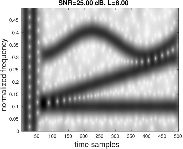
In this experiment, we consider a synthetic -sample-long multicomponent real-valued signal made of two impulses, one sinusoid, one chirp and one sinusoidally modulated sinusoid. Fig. 1 compares the following tfrs: spectrogram, reassigned spectrogram, classical (frequency-reassigned) synchrosqueezing, second-order vertical synchrosqueezing, time-reassigned synchrosqueezing and second-order time-reassigned horizontal synchrosqueezing. Our computations use , and a snr (snr) equal to 25 dB obtained by the addition of a Gaussian white noise. The local modulation estimator is used for computing both second-order synchrosqueezing methods. The tfrs provided by the previously proposed methods are computed using the matlab implementions provided by the ASTRES toolbox [16].
The results clearly illustrate the improvement of the new second-order time-reassigned synchrosqueezing over the time-reassigned synchrosqueezing for representing the whole signal. When compared with frequency-reassigned synchrosqueezing methods, our new method has the advantage to perfectly localize the two impulses while providing a sharpened representation of the chirp and of the sinusoidally modulated sinusoid. Unfortunately, as for the time-reassigned synchrosqueezing, our method cannot localize the non-modulated sinusoid.
To assess the signal reconstruction capability, we compare in Table 1 the rqf (rqf) of each tfr computed using [15]: . Thus, our results show again the advantage of the time-reassigned synchrosqueezing methods which obtain significantly higher rqf (if is chosen at least equal to the signal length) due to its theoretically exact reconstruction formula.
| Method | RQF (dB) |
|---|---|
| STFT | 269.27 |
| classical synchrosqueezing | 35.89 |
| second-order vertical synchrosqueezing | 23.80 |
| time-reassigned synchrosqueezing | 116.67 |
| second-order time-reassigned synchrosqueezing | 116.67 |




4.2 Draupner wave signal analysis
Now we consider a record of a possible freak wave event measured on the Draupner Platform in 1995 [23]. The signal displayed in Fig. 2(a) corresponds to the sea surface elevation deduced from the measures provided by a wave sensors consisting of a down-looking laser. The sampling frequency of this signal is Hz and its duration is 20 minutes.
4.2.1 Time-frequency representation
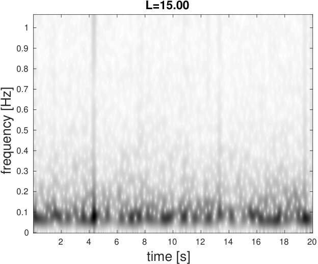
Fig. 2 compares the resulting tfrs provided by the stft and its different synchrosqueezed versions (i.e. all the combination of the first- and second-order of the frequency-reassigned and time-reassigned). For our numerical results, we empirically choose and which provide sufficiently readable results. In order to focus to the impulsive part of the signal, we have limited the analysis between 0.2 Hz and 1 Hz. As expected, the second-order time-reassigned synchrosqueezing provides the best representation to localize the 4 impulses visible in the signal. Interestingly, our results reveal the main impulse located at min (also visible in Fig. 2(a)) but also 3 supplementary impulses respectively located at min, min and min. These impulses were almost invisible in the waveform representation of the signal but have been revealed by our proposed time-frequency analysis methods.
4.2.2 Impulses detection and disentangling
Now we propose to use the synchrosqueezing signal reconstruction capability for recovering the 4 impulse signals. To this end, we compute a saliency function defined as the root mean square of the marginal over frequency band Hz of the signal energy contained in its synchrosqueezing transform:
| (24) |
A binary masked version of the transform can thus be computed using as:
| (25) |
where is a defined threshold. Finally the components are extracted by applying the reconstruction formula given by Eq.(14) on . Our numerical computation presented in Fig. 3 uses which corresponds to 5 times the mean value of . It allows us to recover the impulses locations through a peak picking and to reconstruct the corresponding waveform signal initially merged in the whole signal.
5 Conclusion and future work
A new extension of the time-reassigned synchrosqueezing called second-order horizontal synchrosqueezing was introduced for the stft. Our experiments show a significant improvement to compute invertible and sharpened time-frequency representations of impulsive signals which cannot be addressed by vertical synchrosqueezing. Moreover, we have shown the efficiency of this technique when applied on both synthetic and real-word signals. In fact, our method helped to discover new signal components in the Draupner wave signal which could probably help to better understand the phenomenon of freak waves. Future work consist in theoretically strengthening this method, and developing new applications.
Acknowledgment
The authors would like to thank Dr. Sverre Haver who kindly agreed to answer our questions and share with us the Draupner wave signal record.
References
- [1] L. Cohen, Time-Frequency Analysis: Theory and Applications. Prentice Hall, 1995.
- [2] P. Flandrin, Time-Frequency/Time-Scale analysis. Acad. Press, 1998.
- [3] F. Hlawatsch and F. Auger, Eds., Time-Frequency Analysis: Concepts and Methods. ISTE-Wiley, 2008.
- [4] P. Flandrin, Explorations in Time-Frequency Analysis. Cambridge University Press, 2018.
- [5] A. Grosssmann and J. Morlet, “Decomposition of Hardy functions into square integrable wavelets of constant shape,” IAM Journal of Mathematical Analysis, vol. 15, no. 4, pp. 723–736, 1984.
- [6] A. Klapuri and M. Davy, Eds., Signal Processing Methods for Music Transcription. Springer US, 2006.
- [7] K.-K. Poh and P. Marziliano, “Analysis of neonatal EEG signals using Stockwell transform,” in Engineering in Medicine and Biology Society, 2007. EMBS 2007. 29th Annual International Conference of the IEEE, Aug. 2007, pp. 594–597.
- [8] K. Kodera, R. Gendrin, and C. de Villedary, “Analysis of time-varying signals with small BT values,” IEEE Trans. Acoust., Speech, Signal Process., vol. 26, no. 1, pp. 64–76, Feb. 1978.
- [9] F. Auger and P. Flandrin, “Improving the readability of time-frequency and time-scale representations by the reassignment method,” IEEE Trans. Signal Process., vol. 43, no. 5, pp. 1068–1089, May 1995.
- [10] I. Daubechies, J. Lu, and H.-T. Wu, “Synchrosqueezed wavelet transforms: An empirical mode decomposition-like tool,” Applied and Computational Harmonic Analysis, vol. 30, no. 2, pp. 243–261, 2011.
- [11] F. Auger, P. Flandrin, Y. Lin, S. McLaughlin, S. Meignen, T. Oberlin, and H. Wu, “TF reassignment and synchrosqueezing: An overview,” IEEE Signal Process. Mag., vol. 30, no. 6, pp. 32–41, Nov. 2013.
- [12] D.-H. Pham and S. Meignen, “A novel thresholding technique for the denoising of multicomponent signals,” 2018.
- [13] P. Flandrin, “Time–frequency filtering based on spectrogram zeros,” IEEE Signal Process. Lett., vol. 22, no. 11, pp. 2137–2141, 2015.
- [14] D. Fourer and G. Peeters, “Fast and adaptive blind audio source separation using recursive levenberg-marquardt synchrosqueezing,” in Proc. IEEE ICASSP, Calgary, Canada, Apr. 2018.
- [15] D. Fourer, F. Auger, and P. Flandrin, “Recursive versions of the Levenberg-Marquardt reassigned spectrogram and of the synchrosqueezed STFT,” in Proc. IEEE ICASSP, Mar. 2016, pp. 4880–4884.
- [16] D. Fourer, J. Harmouche, J. Schmitt, T. Oberlin, S. Meignen, F. Auger, and P. Flandrin, “The ASTRES toolbox for mode extraction of non-stationary multicomponent signals,” in Proc. EUSIPCO 2017, Kos Island, Greece, Aug. 2017, pp. 1170–1174.
- [17] T. Oberlin, S. Meignen, and V. Perrier, “Second-order synchrosqueezing transform or invertible reassignment? Towards ideal time-frequency representations,” IEEE Trans. Signal Process., vol. 63, no. 5, pp. 1335–1344, Mar. 2015.
- [18] D. Fourer, F. Auger, K. Czarnecki, S. Meignen, and P. Flandrin, “Chirp rate and instantaneous frequency estimation: application to recursive vertical synchrosqueezing,” IEEE Signal Process. Lett., 2017.
- [19] D. H. Pham and S. Meignen, “High-order synchrosqueezing transform for multicomponent signals analysis-with an application to gravitational-wave signal.” IEEE Trans. Signal Processing, vol. 65, no. 12, pp. 3168–3178, 2017.
- [20] D. He, H. Cao, S. Wang, and X. Chen, “Time-reassigned synchrosqueezing transform: The algorithm and its applications in mechanical signal processing,” Mechanical Systems and Signal Processing, vol. 117, pp. 255–279, 2019.
- [21] R. Behera, S. Meignen, and T. Oberlin, “Theoretical analysis of the second-order synchrosqueezing transform,” Applied and Computational Harmonic Analysis, Nov. 2016.
- [22] D. Fourer, F. Auger, and G. Peeters, “Local AM/FM parameters estimation: application to sinusoidal modeling and blind audio source separation,” IEEE Signal Processing Letters, vol. 25, pp. 1600–1604, Oct. 2018.
- [23] S. Haver, “A possible freak wave event measured at the draupner jacket january 1 1995,” in Rogue waves, vol. 2004, 2004, pp. 1–8.