Spatial patterns emerging from a stochastic process near criticality
Abstract
There is mounting empirical evidence that many communities of living organisms display key features which closely resemble those of physical systems at criticality. We here introduce a minimal model framework for the dynamics of a community of individuals which undergoes local birth-death, immigration and local jumps on a regular lattice. We study its properties when the system is close to its critical point. Even if this model violates detailed balance, within a physically relevant regime dominated by fluctuations, it is possible to calculate analytically the probability density function of the number of individuals living in a given volume, which captures the close-to-critical behavior of the community across spatial scales. We find that the resulting distribution satisfies an equation where spatial effects are encoded in appropriate functions of space, which we calculate explicitly. The validity of the analytical formulæ is confirmed by simulations in the expected regimes. We finally discuss how this model in the critical-like regime is in agreement with several biodiversity patterns observed in tropical rain forests.
I Introduction
Several authors have showed that the parameters of models which describe biological systems are not located at random in their parameter space, but are preferably poised in the vicinity of a point or surface which separates regimes of qualitatively different behaviors mora2011biological. In this sense, stationary states of living systems are not only far from equilibrium, but bring the hallmark of criticality. Although the connection between underpinning dynamics and measurable quantities is sometimes tenuous and hence conclusions about criticality loose, empirical examples span a wide range of biological organization, from gene expression in macrophage dynamics nykter2008gene, to cell growth furusawa2012adaptation, relatively small networks of neurons schneidman2006weak, flocks of birds cavagna2010scale and, possibly, tree populations in tropical forests tovo2017upscaling.
In this article, we mainly focus on the spatial patterns emerging from a minimal model of population dynamics close to its critical point. This latter is identified as a singularity in the population size of the system, similarly to what happens in the theory of branching processes in the sub-critical regime athreya2004branching, when the fluctuations play a crucial role. Therefore, in our model the critical point does not mark a transition between ordered and disordered phases sensu equilibrium statistical mechanics cardy1996scaling, although connections in a broader context may certainly exist. The emergent patterns are not calculated by using classical size-expansion methods, but introducing a parameter expansion which appropriately identifies criticality in the parameter space of the model.
The calculation of the probability distribution of large scale configurations emerging from the microscopic dynamics is challenging, even at stationarity jahnke2007solving; mellor2016characterization. When stochastic processes violate detailed balance, they have a generator which is not self-adjoint pavliotis2014stochastic and different states are coupled by probability currents at microscopic level zia2007probability. These flows of probability among microstates break detailed balance, time symmetry and produce macroscopic non-equilibrium behavior. A common way to overcome these hurdles is to formulate some kind of effective Langevin equation which describes the dynamics of the mesoscopic variables of interest, loosing track, however, of the underlying microscopic dynamics henkel2008non; garcia2012noise; shem2017solution. Nonetheless, in this paper we study a model which, despite violating microscopic detailed balance krapivsky2010kinetic; grilli2012absence, allows one to study analytically (stationary) out-of-equilibrium properties of spatial patterns. These latter emerge mainly because of the large intrinsic fluctuations of the local population sizes. Also, the model’s mathematical amenability allows us to analyze in detail those spatial ecological patterns and to compare them with observation data for ecosystems with large species richness. The agreement between model predictions and empirical data highlights the usefulness of the approach and strengthens the connections between physics and theoretical ecology.
In this spatial metacommunity model, local communities (or, equivalently, sites or voxels) are located on a -dimensional regular graph (or lattice) where individuals are treated as well-mixed particles which undergo a birth and death process with local diffusion and constant colonization. We thoroughly investigate the spatial stochastic dynamics close to criticality and deduce the equation governing the evolution of the conditional distribution , the probability to find individuals in a volume at time (in dimension ). Within this regime we map the equation of of the out-of-equilibrium spatial model into an equation of a suitable stochastic process, which instead satisfies detailed balance. This model is described by functions of space, which we are able to calculate exactly. The exact stochastic simulations are always matched by our analytical formulæ in the expected regimes.
The rest of the paper is organized as follows: in section II we introduce the master equation of the model; in section III we calculate the mean and pairwise correlation; in section IV we study the generating function of the conditional probability density function of ; in section V and VI we calculate the population variance and the conditional pdf of , respectively, along with a comparison between simulations and analytical formulæ; in section VII we present an ecological application of the model; finally, section VIII includes some discussions and perspectives about the results.
II Master equation of the model

This is a metapopulation model in which individuals live in local communities (or sites) located on a -dimensional lattice, , whose linear side is . If , , indicates an individual living in site , the reactions defining the model’s dynamics can be cast into the form
where indicates a site which is a nearest neighbor of the site . In this model, individuals within local communities (or, equivalently, sites or voxels) are treated as diluted, well-mixed point-like particles which undergo a minimal stochastic demographic dynamics: each individual may die at a constant death rate and give birth to an offspring at a constant rate . The newborn individual remains in the same community with probability , whereas it may hop onto one of the 2 nearest neighbours with probability . Also, all communities are colonized by external individuals at a constant immigration rate , which prevents the system to end up into an absorbing state without individuals o2010field; o2018cross.
Notice that (for ) spatial movement is always coupled to birth, so that only newborn individuals can move. This is because we have in mind an application to spatial ecology, where this model mimics the population dynamics in species-rich communities of trees, in which only seeds can move. However, it can be easily modified to include random walk behaviour or different dispersals – like those for bacteria or humans – in which the local birth and the hopping probability are in general decoupled. We have indeed verified that the generality of our final results does not depend on that coupling (see Appendix F).
In the language of chemical reaction kinetics, the first reaction represents an autocatalytic production; this and the hopping move are responsible for the break of detailed balance as shown in Appendix A. Therefore, stationary states of this process are non-equilibrium steady states, albeit the model is defined by linear birth and death rates.
Indeed, it is worth emphasizing that each “patch” has not a maximum number of individuals which it can accommodate, but any population size is allowed, albeit large sizes have an exponentially small probability to occur. This is because the model has no intrinsic carrying capacity which leads the population to saturation. A carrying capacity has the advantage to bring in more realistic features, but it also makes the model mathematically more complicated because of non-linear terms. Here we show that linear rates of a stochastic model per se can produce a relevant phenomenology within a stationary out-of-equilibrium model. Thus, since we wanted to focus on the regime near criticality, we have preferred to delve into a relatively simpler system, in which non-linearities are neglected in a first approximation. More complicated dynamics are definitely important and will be studied in future works.
Finally, for the system to avert demographic explosion we have to assume that and , but it turns out that the most interesting features emerge when , i.e., close to its critical point. Indeed, as we will show in Section VII, for comparable birth and death rates the model is able to describe several spatial patterns of tree species in tropical forests azaele2016statistical.
Let us now indicate with the number of individuals in site . Assuming that within every site the spatial structure can be neglected and that we have perfect mixing, when the configuration of the system is , the linear birth and death rates in site , i.e., and , read respectively
| (1) |
Let be the probability to find the system in the configuration at time . Then the master equation for reads
| (2) | ||||
where the dots represent that all other occupation numbers remain as in and it is intended that whenever any of the entrances is negative. The spatial generating function of the process is defined as
| (3) |
where for every . Multiplying both sides of eq.(2) by and summing over all configurations of the system, we find that satisfies the equation
| (4) | ||||
This is the main equation of the model from which we will calculate the most important results. We were not able to find the full solution of this equation. However, one can gain a lot of information about the general properties of the process by looking into the probability distribution of the random variable , where is the set of sites in a -dim volume. Before studying such a distribution, it is useful to calculate the mean number of individuals and the spatial correlation between any pair of sites.
III Mean and Pair Correlation
The equation for the mean number of individuals in the site can be obtained by taking the partial derivative of both sides of eq.(4) with respect to and then setting :
where and is the discrete Laplace operator, which is defined as
This finite difference equation can be solved in full generality and at stationarity, i.e. for , we get simply , regardless of any spatial location.
The pairwise spatial correlation between sites and , i.e., , can also be obtained by taking the partial derivatives of both sides of eq.(4) with respect to and , and then setting (see Appendix B for details):
| (5) | ||||
where we have used the notation
We also introduce
which are dimensionless parameters and provide important information about how spatial diffusion intermingles with demographic dynamics.
In order to solve eq.(5), we introduce a -dim system of Cartesian coordinates where the coordinates of each site are given as a multiple of the lattice side . Thus, a vector k indicates the corresponding position of a site. In this way, we can calculate the stationary solution of eq.(5) by writing as a Fourier series expansion. Exploiting translation invariance the final expression of the solution reads (see Appendix B)
| (6) |
where is the -th Cartesian component of the -dim vector p and is the hypercubic primitive unit cell of size . Interestingly, pairs of sites de-correlate for or , when at stationarity we obtain , where is a constant depending only on the demographic parameters and is a Kronecker delta. However, , pointing out that local fluctuations are non-Poissonian.
Eq.(6) is amenable to a continuous spatial limit, obtained as , and provides a closed analytic form for the pair correlation. Indicating now with and the density of individuals on the sites located at and , respectively, in continuous space (and rescaling parameters accordingly), we find (see Appendix B)
| (7) | ||||
where is the distance between the sites located at and , is the modified Bessel function of the second kind of order lebedev2012special, and we have defined
where and for , and they are assumed to be finite in the limit. The first one is a standard scaling for spatial diffusivity, whereas the second scaling assumption comes from the requirement that spatial continuous constants are finite and non-trivial as for .
As the asymptotic behavior of as is , is the correlation length of the system; has the dimensions of a -dim volume and gives the local intensity of the correlations. Because eq.(7) is the continuum limit of eq.(6), this expression of the pair correlation function is a good approximation of the one in eq.(6) only when and .
IV Generating function close to the critical point
In this section we introduce the parameters which allow us to identify a region close to the critical point of the model. This suggests an expansion which will lead to simplified equations which, nonetheless, carry a lot of information about the model.
A simple way to make progress with the master equation in eq.(2) is the use of a formal Kramers-Moyal expansion gardiner2004handbook. It is well-known that there are limitations to this procedure and it has been criticized, because one cannot always pinpoint a small parameter for the correct expansion gardiner2004handbook; van1992stochastic. The system-size expansion solves these difficulties, but it has to be applied when the size of the system becomes large van1992stochastic. Here, however, it is not entirely evident what parameter should identify the size (population size or volume) of the system in the critical regime. Indeed, the model has no carrying capacity or maximum population size, and the total volume of the system could only provide us with the macroscopic equation, which has no interest in the present case.
In order to make analytical progress, we have introduced two dimensionless parameters, and , which identify a non-trivial region when , but . This choice comes from the observation that communities of living organisms often appear to have very large demographic fluctuations. Several studies (see Volkov2005; Volkov2007; tovo2017upscaling) have pointed out that per capita birth and death rates are close to each other in seemingly different systems, thus suggesting that a sensible theoretical limit to study is when approaches . For example, a fit of eq.(7) to the empirical two-point correlation function of the tropical forest inventory of Pasoh natural reserve in Malaysia leads to empirical values of of the order of (see Fig. (4) and section VII for more details). We hence define with the condition that as ; in this way we obtain a constant , which in real systems is large because usually . The parameter indicates how close the system is to the critical point, regardless of spatial diffusion. With the independent parameter , instead, we compare the importance of spatial diffusion with respect to demographic fluctuations. We will assume that as and hence , a new independent constant. This scaling assumption reflects that we want to explicitly analyze spatial effects in the critical limit. In fact, it can be easily proved that when , the model is equivalent to the mean field model without spatial diffusion, whereas for spatial diffusion dominates over the birth-death dynamics.
When and are close to each other, we expect that population sizes can be well approximated with continuous random variables in each site. In order to understand when this is possible in relation to the parameters and , we assumed that the generating function is analytic at for any and the most important contribution to the equation of comes from a negative neighborhood of the origin with thickness . This is tantamount to introducing the change of variable into eq.(4) and to expanding in powers of , assuming and . Up to linear order in and we obtain
| (8) |
or
| (9) |
where we have introduced the dimensionless time and now , with a slight abuse of notation, indicates the generating function corresponding to continuous (and dimensionless) random variables. Therefore, the evolution equation for the generating function of the population sizes becomes
| (10) |
where is the variable conjugated to the continuous random variable . The parameters also correspond to this continuum limit and now the population sizes have an exponential cut-off with a (large) characteristic scale given by . Eq.(10) leads to the following Fokker-Planck equation:
| (11) |
where now are continuous random variables and is the corresponding probability density function. It is interesting to note that this is not exactly equivalent to the naïve Kramers-Moyal expansion of eq.(2), which would entail additional terms in the diffusive part. Nevertheless it is a diffusive approximation of the process in the regime identified by the parameters and .
IV.1 Conditional generating function
Eq.(IV) cannot be solved in full generality, but we can better understand the underlying dynamics by studying the distribution of the population sizes in arbitrary volumes of space. Let us indicate with the set of sites belonging to a -dim volume , and let us introduce the random variable , i.e. the total number of individuals in at time . By indicating with the corresponding probability density function of , we define the conditional generating function
where . We obtain the corresponding equation for by specifying , i.e.
| (12) |
and substituting this into eq.(10). Thus,
| (13) | ||||
where and we have used the identity
| (14) |
This equation depends on which in general is unknown. An equation for can be derived by differentiating both sides of eq.(10) with respect to . Assuming as before that , we finally obtain the following equation for (abbreviated )
| (15) | ||||
where and where we have used the identity
| (16) |
In eq.(15) the function is still unknown, but it is possible to show that to leading order as (see Appendix C). This allows us to obtain a closed equation for . Indeed, we have
after using the identity (16).
The spatial continuous limit of eq.(13) as reads
| (17) | ||||
where in we have substituted with . This equation is of crucial importance in what follows. Similarly, eq.(15) becomes
| (18) | ||||
where with the continuous coordinates ( and ), we have also and . When there are no spatial effects, i.e., , eq.(17) reads
| (19) |
which has the following solution at stationarity
| (20) |
where and . This is the generating function of a gamma distribution van1992stochastic with mean and variance . Also, it is not difficult to verify that when , the solution of eq.(18) is given by
| (21) |
In the next section we calculate the stationary variance of the population sizes in a volume , i.e., of the random variable .


V Population Variance
In this section we calculate the stationary variance of the population size, i.e., , where is a finite volume. This quantity is of pivotal importance in the approximation that we are going to develop in the following sections and it is key when introducing spatial information in the equations. Thus we outline here the main calculations, leaving to Appendix D further details.
We start from the spatial continuous limit of eq.(5) as , which at stationarity reads
| (22) |
where is a Dirac delta and we have included only the leading terms as . By integrating both sides of eq.(22) with respect to , we obtain an equation for . We plan to find an explicit expression for this quantity, because it plays a key role in the following when we will calculate . Henceforth, we will take to be a -dim ball of radius and we will assume that the origin of the Cartesian coordinates is at its center. Thus we indicate with the distance from the origin of the site located at in this coordinate system. With this notation and using the symmetry of with respect to and , we obtain at stationarity
| (23) | ||||
This linear ODE has to be solved separately for and . The continuity of and its first derivative at the boundary provide the solution. The final results is (see Appendix D)
| (24) |
where the function takes the following form for
| (25) | ||||
where and are the modified Bessel functions of the first and second kind, respectively lebedev2012special. Integrating both sides of eq.(24) with respect to , we obtain the equation for the second moment of , i.e.
| (26) |
where takes the following explicit form in dimension (see Appendix D for its behavior):
| (27) |
These two functions, namely in eq.(24) and in eq.(26) will be used in the next sections to calculate a first order approximation of the spatially explicit probability density function of in the vicinity of the critical point.
Finally, these solutions allow us to write down the analytic form of the variance of in dimension , i.e.
| (28) |
where and . The function is the spatial Fano factor and quantifies the deviations of the fluctuations from a Poisson process. Since , when the system is close to the critical point – for fixed and – the system has large fluctuations on all scales larger than the correlation length . Also, in the regime we obtain , thus recovering the mean-field fluctuations as predicted by eq.(20).
V.1 The spatial Taylor’s law
Taylor’s law was first observed in ecological communities taylor1961aggregation; taylor1977aggregation, where natural populations show some degree of spatial aggregation. This was phenomenologically captured by assuming a scaling relationship between the variance and mean of population sizes in different areas. More generally, and recently, Taylor’s law denotes any power relation between the variance and the mean of random variables in complex systems eisler2008fluctuation; james2018zipf. The law postulates a relation of the following form
where is a positive constant and typically assumes values between one and two taylor1977aggregation; james2018zipf. The spatial model which we have introduced can predict the behavior of this relation across scales without making specific assumptions. If we focus on the two dimensional case and fix , we obtain for , while for . This latter situation corresponds to the mean field case in which . So for areas of radius much smaller than the correlation length the model is characterized by with logarithmic corrections, while in the case of radii much larger than we obtain . This is in agreement with previous studies taylor1961aggregation; taylor1977aggregation; eisler2008fluctuation. The model predicts at large scales regardless of the dimension of the system, whereas for small areas strongly depends on , e.g. (without logarithmic corrections) in the one dimensional case, and for . Therefore, from small to large spatial scales the model predicts a cross-over of exponents which is difficult to explain without a spatially-explicit framework. Recently, considerable attention has been devoted to the origin of curvatures in scaling relationships, such as those relating body size and the metabolic rates of living organisms (e.g species of mammals r01748 or freshwater phytoplankton Zaoli17323). Unlike what has been found in these latter works, in our model the cross-over in the scaling exponent is a result of the interplay between space and dispersal at different spatial scales. When considering small areas, local communities appear strongly correlated with each other, while at larger areas these communities are completely independent as they are located at distances much larger than the correlation length. When they are decoupled, the relation is simply , where is the volume of a -dimensional sphere.
It has been proved that Taylor’s law can emerge in a much more general class of stochastic processes, for example when the dynamical rates of the model are affected by environmental variability eisler2008fluctuation; james2018zipf. Here we do not consider this effect, but it would be certainly interesting to investigate environmental stochasticity within a spatially explicit framework.
VI Solution of the conditional pdf
The goal of this section is to derive the main result of the paper. With the spatial population variance obtained in the previous section along with an appropriate approximation, we are now able to close and solve eq.(17) for the conditional generating function . We will then invert this latter for the conditional probability density function , from which several characteristics of the spatial patterns can be deduced.
In order to calculate the explicit form of from eq.(17), we first need to calculate the solution of eq.(18), which in turn has to satisfy the identity in eq.(14). We will first make use of this latter in the form
| (29) |
It is not difficult to verify that can be expressed as
| (30) |
where the functions are such that
| (31) |
for any . One could calculate the explicit form of , which depends on the spatial position, by substituting the expression in eq.(30) into eq.(18). However, the meaning of these functions provides a more efficient way for the calculation. Because of the definition of , we readily obtain and
| (32) |
for , from which we can make explicit the expression of by using eq.(30). For instance, it is not difficult to show (see Appendix E) that at stationarity
where and have been defined in eqs.(25) and (27), respectively. Similar relations, though more complicated, hold for . Actually, can be calculated by integrating times over the volume the -th spatial correlation function. Nonetheless, note that this result depends on the symmetry of the -dim volume , and on its connectedness. This is important for exploiting the spherical symmetry of the system when introducing polar coordinates, and in selecting its center as the origin (see also the previous section and Appendix D) .
Since we are interested in relatively large population sizes when the correlation length is either large or small ( but finite), we retain only the first two terms in the bracket of eq.(30). Thus, at stationarity turns into
| (33) |
where is the one we have obtained before. It is remarkable that, when substituting eq.(33) into eq.(17), at stationarity one obtains (see Appendix E)
| (34) |
where is the spatial Fano factor defined in the previous section. The form of eq.(34) and that of eq.(19) at stationarity are the same, provided we replace with . Therefore the solution of eq.(34) is
| (35) |
which, when inverted for the probability density function, gives a gamma distribution of the form
| (36) |
Thus, while without spatial effects the characteristic scale of the population size is , in this regime space introduces a space-dependent scale for fluctuations which is quantified by , where is the function defined in eq.(27).
As a further insight, if one defines the new process for the random variable in the volume of fixed radius by the stochastic differential equation
| (37) |
where is a zero-mean Gaussian white noise and , then the stationary pdf of is exactly eq.(36). Notice that space is taken into account only implicitly through the functions and . Eq.(37) can also be obtained as an -limit of a spatially-implicit master equation along the lines we have showed in Section IV. This process – unlike the spatial one – satisfies the detailed balance condition at stationarity as the flux at is set to zero. This result suggests that there are some families of spatially-explicit processes which, when restricted to a finite volume, can be well approximated by spatially-implicit processes. Whilst the former brakes detailed balance, the latter turns out to be simpler and satisfies the detailed balance condition. In this model the region of this approximation is close to the critical point of the process.
It remains to understand when the in the form of eq.(33) solves eq.(18), i.e. the original equation for . In Appendix E we show that, for a fixed radius , at stationarity is a solution when is small and is either very large or very small (but finite) compared to , regardless of the spatial dimension . The limits and of eq.(36) lead to the mean-field expressions, respectively eq.(19) and at leading order. Thus, eq.(36) captures the leading behavior of the distribution of the random variable in the large population regime and in the vicinity of the critical point. The simulations indeed confirm this with very good accuracy as shown in Figs.(2) and (3).
Because we assumed that is at stationarity, eq.(33) does not give all the correct terms for a time evolution of the process . However, relatively close to stationarity, even the temporal dynamics is accurately described by eq.(37). We have checked this idea and compared the exact simulations of the process – as provided by the Doob-Gillespie algorithm (see also the following section) – with the corresponding analytic temporal evolution as obtained from solving eq.(37). Assuming that initially in the volume there are individuals, we find the following time-dependent solution (see azaele2006dynamical for the details of the derivation):
| (38) | ||||
where we used reflecting boundary conditions at at any . This pdf indeed tends to the stationary solution in eq.(36) as . The agreement between simulations and eq.(38) is showed in Fig.(7) and (8).
Simulations with an efficient algorithm
These families of spatial stochastic models are difficult to simulate with parameters in arbitrary regimes and even so, usually only on relatively small lattices in low dimensions. Indeed, it is difficult to assess whether or not simulations have reached stationarity (because of the effect of large fluctuations) and how many replicates are necessary to get reliable predictions for the spatial moments. In this light, it is even more important to know the analytical behavior of some quantities, which could not have been guessed from the simulations only. We have therefore compared our analytic predictions to simulations as obtained from a range of different parameter sets and from two different simulation schemes.
The first one is the Doob-Gillespie’s algorithm Gillespie1977exact for producing exact trajectories of Markovian processes. We have used periodic boundary conditions in 1- lattices of various sizes. Parameters were chosen so that the correlation length of the system was much smaller than the total size of the lattice. We have analyzed different sets of parameters and for each one we have run 50,000 independent realizations: error bars were calculated by grouping the results into 50 sets made of 1000 realizations each. In principle this simulation scheme allows us to obtain the exact trajectories of the system at any time, from an initial configuration up to stationarity. However, it is computationally very expensive, and therefore we have been forced to choose relatively small lattice sizes to investigate significant changes from the initial configuration. The results of this are shown in Figs.(7) and (8).
In order to analyze a wider set of parameters and larger lattices, we have simulated the process by using a new algorithm which generates the stationary random field obtained from the stochastic partial differential equation defined on the lattice. This was introduced in peruzzo2017phenomenological, and modifies a previous scheme that was used for simulating models of directed percolation Dornic2005integration. Here we briefly summarize the main steps of the pseudo-code. From the definition of the discrete Laplace operator, we split the term in eq.(IV) into one part depending only on () and another one depending on the densities in the nearest neighboring sites (). Conditional on the values of for , the second term is constant and thus can be obtained as a gamma distribution at stationarity peruzzo2017phenomenological. Starting from a random initial configuration, at each iteration , we randomly select a site and update the value of in the next step by sampling from , conditional on the values of (i.e. ). These steps are repeated until lattice configurations become independent of initial conditions. While standard stochastic integration schemes fail to preserve the positivity of at any step, this algorithm produces non-negative populations by construction. We have verified that the simulated distribution thus obtained for matches the exact simulations of the Doob-Gillespie’s algorithm in and for different lengths, when the comparison was feasible (see Fig.(9)). By means of this algorithm we were able to study much larger lattice sizes at stationarity, and compare simulations against the predictions of the analytic solutions. The agreement was excellent in all the expected regimes (see Figs.(2) and (3)).
VII An ecological application


A simple, but far from trivial, application of the mathematical model we have previously described is the modelling of spatial patterns in ecosystems with a large number of species. Examples include the species richness and abundance distribution of coral reefs, bees across landscapes or vascular plant species in tropical forest inventories. Starting with the crude approximation that species are independent (at least at some relatively large scale), this model can be used to predict the abundance distribution of species from measures of the two-point correlation function (PCF) and mean abundance per species. Because these latter descriptors are relatively easy to calculate, it turns out that we can obtain an estimate of how many rare (or abundant) species live in a region without surveying the entire system. Therefore, as well as being theoretically interesting, this approach has also an important practical advantage, because it ultimately allows one to infer the total number of species within a very large spatial region by utilizing only scattered and small-scale samples of the region itself. This is a long-lasting problem which has received a lot of attention recently tovo2017upscaling; shem2017solution; azaele2016statistical.
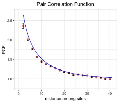
Our goal here is not to explain the upscaling method, but only show to what degree the spatial model is in agreement with ecological empirical data. The two-point correlation function (PCF) specifies how similar individuals are distributed as a function of the geographic distance. Since species are assumed to be independent, the spatial distribution of individuals belonging to the same species can be considered as an independent realization of the stochastic process. As a consequence, the term in eq.(7) can be easily calculated as the product of local abundances of individuals in sites that lay at the same distance, averaged across all species. Usually, it is more likely that close-by individuals belong to the same species than individuals that live farther apart. This translates into a PCF that is always positive, but decays with distance condit2002beta; chave2002spatially. A decline in similarity with increasing geographic distance indicates that the individuals of a community are spatially aggregated. Therefore, a simple random placement of individuals in space is not a good approximation of the configurations of the community as thought in the past coleman1981random. On the contrary, the stationarity PCF of this model decays with distance, is always positive (see eq.(7)) and has two free parameters ( and ). When we calculate these latter from a best fit of the empirical data, we obtain a good agreement as shown in Fig.(4d).
The mean abundance per species is readily available, because the total number of species and individuals are known in this forest plot. Since at stationarity the model is fully specified by these three parameters (, and ), we are henceforth able to predict all the stationary patterns that we like to compare with those of the empirical ecosystem. One of them is the probability that a species has a given number of individuals within a specific region. In the ecological literature it is often referred to as species abundance distribution (SAD) mcgill2007species. In our model it is given by eq.(36) and the histograms of this pattern are reported in Fig.(4a-c) for different radii. The SAD represents one of the most commonly used static measures for summarizing information on ecosystem’s diversity. Interestingly, the shape of the SAD in tropical forests has been observed to maintain similar features, regardless of the geographical location or the details of species interactions. Indeed, it often displays a unimodal shape at larger scales and a peak at small abundances at relatively small spatial scales. Numerous papers have focused on evaluating the processes that generate and maintain such observed characteristics black2012stochastic; azaele2016statistical, but only few of them considered spatial effects in an explicit framework pigolotti2018stochastic; o2018cross.
The panels in Fig.4 show a comparison between the empirical data from the forest inventory of Pasoh Natural reserve in Malaysia (year 2005) and the predicted abundance distribution of species obtained from the model we have described in the previous sections. It is remarkable that the predicted curves in the first three panels are genuine inferences obtained from the mean abundance per species (i.e., ) and the PCF (i.e., and ), and not best fitted curves to empirical SAD. As a comparison, we have included the best fit to data of a probability distribution commonly used as null model in the literature, the Fisher log-series (see Appendix G) azaele2016statistical. The two methods have comparable accuracies at smaller scales, while at larger scales our method outperforms the Fisher log-series and captures the empirical SAD with much higher accuracy.
Such an agreement confirms that abundances of species are indeed characterized by very large fluctuations and that local populations appear correlated over very large spatial scales. This entails that complex ecosystems may comprise a large number of rare species, whereas only a few have large abundances (hyperdominant species). Because this model does not explicitly include interactions nor environmental forcing, we cannot single out which ecological processes bring about this finding. Nevertheless, the model is able to explain this separation of population size scales by poising a system close to criticality.
In terms of new physical insight, the theoretical framework that we have presented here allows us to connect exactly the two-point correlation function to the Species Abundance Distribution (SAD) and the Species Area Relationship (SAR) of a system. This explains quantitatively why and how SAR (known as -diversity in the ecological literature) and species spatial turnover (known as -diversity in the ecological literature) are related. For instance, it is usually assumed that the SAR is a power law function of the area hubbell2001unified, i.e. , however our results show that this can only be an approximation which works on a given range of spatial scales.
The simplicity and generality of the model make it suitable for the description of patterns in other biological systems. Indeed, numerous recent studies have showed that spatial bio-geographical patterns emerge in marine ecosystems rinaldo2002cross; ser2018ubiquitous, microorganisms woodcock2007neutral, including bacteria giometto2014emerging; giometto2015sample, archæa, viruses, fungi hanson2012beyond and eukaryotes altermatt2015big; lynch2015ecology. Future work will include the application of the current framework to those biological communities.
VIII Conclusions
In this paper we have studied a spatial stochastic model which can be fruitfully used to describe the main large scale characteristics of species-rich ecosystems. We have shown how to calculate analytically some of the most important spatial patterns when the system is close to criticality, which is the regime where the most important features emerge.
The model encapsulates birth, death, immigration and local hopping of individuals. It describes the dynamics of point-like and well-mixed individuals living in a metacommunity defined on a -dimensional regular graph. The model is also minimal, meaning that, without one of its components (i.e., birth, death, nearest-neighbor hopping and external immigration), it yields either trivial or well-known results. Despite its simplicity, however, it violates detailed balance (see Appendix A) and generates a remarkable phenomenology of patterns, when the birth and death rates are comparable (criticality), leading to its properties being governed by large fluctuations, whose effect of course escape any classical mean-field analysis. These patterns and fluctuations entail strong correlations on large spatial and temporal scales.
The linearity of the rates is not sufficient to derive a full solution (in a weak sense) of the model. However, in applications one is usually interested in the analytical properties of processes that are much less general than the spatial random field. Thus we restricted our analysis to the conditional distribution, , that individuals are found in a volume . This quantity is sufficiently general to describe a wealth of patterns in several systems. We have found that in the close-to-critical regime, satisfies an aptly derived equation which has the form of the corresponding mean-field equation of the process (i.e., without space). This equation includes functions of , which we have exactly calculated. Such spatial redefinition of the parameters introduces strong deviations from the corresponding mean-field solutions, as confirmed by the exact stochastic simulations. Also, this shows that the process that governs the random variable satisfies detailed balance in a first approximation and close to the critical point, thus being considerably simpler than the distribution of the random field. This result suggests that not only it is possible to make considerable analytical progress in this model, but there may be other, more general, models close to criticality which can be studied with a similar approach.
Indeed, our results suggest the tantalizing hypothesis that the conditional distribution, , provided by some families of spatial stochastic processes, is described by much simpler processes within a specific region of the parameter space. In our model the region of this approximation is close to the critical point of the process and the distribution of the simpler process holds the same functional shape across all spatial scales. Of course, the hypothesis requires much more scrutiny, especially when spatial models include nonlinear terms which can jeopardize the methods developed here. On the other side, our approach allows for the analysis of several generalizations, including non-local dispersal kernels and different sources of noise (e.g., environmental noise).
On a more applied side, our framework explains how the most important patterns in macro-ecology (e.g., SAR, SAD and PCF) are intrinsically connected with each other (see eqs.(7) and (36) and their relation through in eq.(28)), and also accounts for a cross-over of power law behaviors in the spatial Taylor’s law (see eq.(28)). We have compared the predictions against those of the Fisher log-series, commonly used as “null model” in the ecological literature. Despite the free parameter of the Fisher log-series distribution was calculated directly from the empirical data of the species abundance distribution (best fit) at each spatial scale, our model performed much better (see Fig.4), even though we employed the parameters obtained from the PCF curve, which does not provide information about the distribution of abundances of species. Discrepancies between empirical data and theoretical predictions will potentially inform us on the importance of alternative physical effects which will be included in more realistic models.
We have finally shown that, when applying the model to large ecosystems, species are predicted to display a broad range of abundances as a consequence of the critical regime. Therefore, many of them are rare and only a few are very abundant. These large demographic fluctuations are correlated across large spatial scales as well as over long times, in agreement with several empirical datasets collected in well-known tropical forest inventories peruzzo2017phenomenological; tovo2017upscaling; azaele2015towards.
Of course, these findings do not prove that these biological systems are close to criticality, but suggest that it is worth pursuing that route further. In this article we have not investigated the reasons why those systems look nearly critical, nor how they can operate within such tiny regions of their parameter space. For this, one needs to look into how inter- and intra-interactions dynamically lead living systems towards the correct region, in which states are biologically meaningful – however, see mastromatteo2011criticality; goudarzi2012emergent; stieg2012emergent; hidalgo2014information. Nonetheless, our results could help understand what key factors drive such dynamics, and possibly shed light on the importance and effects of non-linearities among interacting agents.
IX Acknowledgments
FP thanks the NERC SPHERES DTP (NE/L002574/1) for funding his studentship. We thank Amos Maritan for insightful discussions.
Appendix A Broken Detailed Balance
We here recall the main general properties of detailed balance. Let us denote with c the configuration of a generic stochastic process and indicate with the probability that the configuration c is seen at time , given that the configuration at time was (abbreviated ). We introduce , which is the (time-independent) rate to transit from state c to . If we consider Markovian dynamics, the evolution of is given by the following master equation (ME) van1992stochastic; gardiner2004handbook
| (39) |
If it happens that for all configurations (this is the detailed balance (DB) condition), then the probability distribution is also a stationary solution of the ME, as we see from eq.(39). On the other hand, it is clear that not all stationary distributions satisfy the detailed balance condition.

It is possible to show zia2007probability that a condition for the validity of DB is that the probability of following a closed path in the space of configurations does not depend on the orientation of the path. More precisely, DB is satisfied if and only if for any choice of a closed path , with an arbitrary number, the following holds
| (40) | ||||
This equation corresponds to microscopic reversibility and, when it is violated, the system can be found in non-equilibrium steady states.
Violation of DB is key to living systems and is the subject of intense recent interest gnesotto2018broken; battle2016broken. In fig. (5) we show with a simple example that for this model the condition in eq.(40) is not satisfied, hence the detailed balance condition does not hold: Fig. (5) shows a path in the space of configurations for which the total rate does depend on the orientation of the closed path. Notice that such counterexample does not hold when spatial dispersal is switched off (i.e. or ), or when autocatalytic production and spatial dispersal rates are equal ().
Appendix B Spatial correlation of the birth-death Markov process
In the main text we have defined the spatial generating function of the model
From eq.(2), multiplying both sides through by and summing over all states, we find eq.(4) of the main text. If we differentiate by and impose , we find the equation for the mean number of individuals , reported in the main text. Taking another derivative with respect to and setting , we obtain the equation for the spatial two-point correlation function (PCF) among the sites and
where , , is a Kronecker delta, and is the discrete Laplace operator as defined in the main text.
Considering stationary patterns, because of homogeneity we have and, introducing , we obtain
We will now consider the Fourier series expansion of , which we will write as
where are the Cartesian coordinates of the locations of sites on the lattice (in units), p is a vector with components which belongs to , the hypercubic -dimensional primitive unit cell of size . Upon substituting in the stationary equation, we get an expression for , which is
where is the -th component of p. Therefore
We can obtain a good deal of simplification by taking a continuous spatial limit (). Renaming , and (now continuous variables in ), and appropriately rescaling the constants as explained in the main text, we arrive at the expression for the pairwise spatial correlation in dim , i.e.
where we have replaced with in and used the definitions of given in the main text. Actually, the -dim integral in the previous expression can be calculated
where is the modified Bessel function of the second kind and in the last step we used 9.6.24 from abramowitz1965handbook. Eventually, the PCF is
| (41) | ||||
Because decays exponentially for large regardless of , plays the role of a correlation length of the spatial system. Instead, has dimensions of a -dim volume and provides a characteristic volume of local demographic fluctuations.


Appendix C Approximating in the continuous spatial limit
Equation (15) shows that the evolution of is not closed, being coupled to the generating function and to the function . In this section we want to show that, at leading order in the limit , the value of approaches . This makes the equation for much simpler, basically decoupling it with the other quantities. For simplicity we will only consider the one dimensional case, but this claim holds true in higher dimensions as well. Thus will be an interval of length and the origin of the coordinate system will be located at its center. By changing slightly the notation, we will now indicate , thus making explicit that extends from site to . Since the system is spatially homogeneous, we can write
As and at leading order, we can neglect in the argument of , thus obtaining
Similarly . Thus, as at leading order we can write
This approximation makes it possible to obtain eq.(18) in the continuous limit.
Appendix D Multidimensional Variance
In the main text we have outlined how to calculate the second moment of the random variable . Here we provide some more details. We will take to be a -dimensional ball with the origin of the Cartesian coordinates in its center. By integrating over in eq.(22) and using the symmetry of in and , we obtain an equation for , which at stationarity reads
| (42) |
where is the Heaviside step function and is the -dim volume
with radius . Eq.(D) must be solved for and separately. Boundary conditions for and its first derivative will fix the values of the integrating constants. For we obtain
while for instead
The constants and will be fixed using the aforementioned continuity conditions. Upon explicit calculation, for we obtain
| (43) |
where was defined in eq.(25) of the main text and and are the modified Bessel functions of the first and second kind, respectively lebedev2012special. Integrating with respect to and using the properties of , we can readily obtain the explicit form of the second moment of , i.e.
| (44) |
where we can read off the explicit expression for , also reported in eq.(27). Finally, since we can explicitly write down the variance of , which takes the form
where . is the spatial Fano factor and quantifies the relative importance of fluctuations in the system. Finally, Fig.(6) shows the behavior of .
Appendix E Evaluation of the regimes of accuracy of the method
In this section we show that the truncation of as in eq.(33) yields an accurate approximation for the conditional probability distribution of the model. By retaining the first two terms in the square brackets of eq.(30), at stationarity we are left with the following
| (45) |
where is the conditional generating function at stationarity. By taking the derivative with respect to of both sides of eq.(45) and setting , we obtain
which gives
Because in Appendix D we have already calculated and (see eqs.(D) and (44)), is known explicitly. Substituting in eq.(45) with obtained before into eq.(17) at stationarity, we get
Now we can readily simplify the term by making use of eq.(D). Integrating this latter with respect to in , since and (see Appendix D), we are therefore left with the following equation
| (46) |
which therefore provides the equation for the generating function of up to terms .
Similarly to what we have done so far, we can get further insight into the evolution of . We substitute from eq.(45) into eq.(18) and use eq.(D) to obtain . Eventually, at stationarity this yields
| (47) | ||||
The first addend of eq.(47) is zero because of eq.(46), and the remaining terms are negligible when is small.
Fixing the values of , and , we can calculate explicitly the regimes of where approaches zero. From eqs.(25) and (27) in the main text it is easy to rewrite as
The asymptotic expansion of the modified Bessel functions is lebedev2012special
when . From this it is not difficult to verify that as we have
and so for indeed .
The case of is more elaborate. Let’s call . After some lengthy but otherwise straightforward calculations we can verify that as we can write
and at leading order is proportional to for .
For the case of let us write . We can verify that
and at leading order is proportional to for . Thus again . These findings follow from that goes into mean-field regimes as (but finite) and hence all spatial terms go to zero.
Appendix F Model with independent dispersal
In this section we show how the analysis that is undertaken in the main text can be extended also to a model where spatial dispersal is independent of birth.
As in the main text, the new model consists of a spatial meta-community where local communities are located on a -dimensional regular graph (or lattice), and within each community individuals are treated as diluted, well-mixed and point-like particles.
The model is defined by the following birth-death dynamics: each individual dies at a constant death rate and gives birth at a constant rate , and communities are also colonized from the outside at a constant immigration rate However, individuals can now jump from one site to any of its 2 nearest neighboring sites at any time (not just after birth), and this happens with rate .
Indicating with , , the individual living in site , the reactions defining the model’s dynamics are the following
where indicates a nearest neighbour of site . Comparison with the reactions reported in section II shows that, indeed, now spatial movement is decoupled from birth events.
Let us now indicate with the number of individuals in site and with the probability to find the system in the configuration at time . The master equation for then reads
| (48) | ||||
where the dots represent that all other occupation numbers remain as in and it is intended that whenever any of the entrances is negative.
Similarly to the procedure followed in the main text, as a first step we introduce the spatial generating function of the model, defined in eq.(3). Multiplying through eq.(48) by and averaging, we obtain the equation for , which reads
| (49) | ||||
The next steps follow exactly the same procedure undertaken in the main text.
Thus, we define the parameter and assume the following parameter scaling: as . We introduce the parameter and fix the scaling as . We further assume that the generating function is analytic at for any and that the most important contribution to the equation of comes from a negative real neighborhood of the origin with thickness . Taking the change of variables , we expand eq.(49) in powers of , assuming and . With the definition of the following constants
which are formally equivalent to those defined in section III, and retaining only the leading order in at eq.(49), we obtain
| (50) |
with the discrete Laplace operator. Dividing through by and rescaling time as we finally obtain
| (51) |
which is exactly equal to eq.(9). Since all the results of this paper stem from this equation (or, equivalently, eq.(10)), the conclusions drawn in the main text for the model with ’seed dispersal’ also hold true for the diffusion model presented in this section, provided the systems are close to the critical point (i.e., as ).
Appendix G A null model: the Fisher Log-series
The Log-series distribution was first proposed in 1943 by the statistician Ronald Fisher to describe the empirical abundance distribution of British moths and Malaysian butterflies fisher1943relation. From a set of assumptions involving the independence of species and the absence of spatial dispersal, Fisher derived the following formula, which provides the probability, , that a species has individuals within an ecosystem:
| (52) |
in which and is a free parameter that is usually determined via a best-fit to data. The Fisher Log-series is still largely used as a null-model in theoretical ecology hubbell2001unified; o2010field, because of the low number of free parameters (only one) and of its straightforward mathematical derivation. Nonetheless, many limitations have emerged azaele2016statistical; o2018cross in more recent years. Among these, the lack of a spatial structure has strongly limited its accuracy in describing spatial ecological patterns.
In Fig.4 we have compared the predictions of our model to the best-fits of eq.(52) (rescaled by the total number of species) for three areas of different sizes. The histograms are -scaled in the -axis, meaning that the -th bin counts the number of species that have abundances between and . In order to compare these empirical data to the analytical predictions, we first need to compute the probability that a species has abundances between and , which is straightforward from eq.(36) and from eq.(52).
Our model at stationarity has a total of three free parameters (namely, , and ). has been obtained directly from the empirical data, whereas and have been calculated from the best fit of the theoretical PCF, i.e. eq.(7), to the empirical PCF, which is unrelated to the species abundance distribution. Once obtained the three parameters, we have predicted the species abundance distribution by using eq.(36), which is the curve showed in Fig.(4) along with the histograms of the empirical data.
Looking at the plots in Fig.(4), we see that our model prediction is very accurate in all three cases, whereas the Fisher log-series fails at fitting the distribution in panels (b) and (c). This is confirmed by standard chi-square analysis: -value in the first panel, and -values of in the other two cases; while the Fisher Log-series yields a -value of and in panels (a) and (b), and of in panel (c). More importantly, our model can predict the SAD at all spatial scales without any further assumptions on the system, whereas a method relying on the fit of eq.(52) introduces new parameters at each spatial scale (which in general are incompatible with each other) and is inapplicable at scales where we do not have empirical data.
References
- [1] Thierry Mora and William Bialek. Are biological systems poised at criticality? Journal of Statistical Physics, 144(2):268–302, 2011.
- [2] Matti Nykter, Nathan D Price, Maximino Aldana, Stephen A Ramsey, Stuart A Kauffman, Leroy E Hood, Olli Yli-Harja, and Ilya Shmulevich. Gene expression dynamics in the macrophage exhibit criticality. Proceedings of the National Academy of Sciences, 105(6):1897–1900, 2008.
- [3] Chikara Furusawa and Kunihiko Kaneko. Adaptation to optimal cell growth through self-organized criticality. Physical review letters, 108(20):208103, 2012.
- [4] Elad Schneidman, Michael J Berry II, Ronen Segev, and William Bialek. Weak pairwise correlations imply strongly correlated network states in a neural population. Nature, 440(7087):1007, 2006.
- [5] Andrea Cavagna, Alessio Cimarelli, Irene Giardina, Giorgio Parisi, Raffaele Santagati, Fabio Stefanini, and Massimiliano Viale. Scale-free correlations in starling flocks. Proceedings of the National Academy of Sciences, 107(26):11865–11870, 2010.
- [6] Anna Tovo, Samir Suweis, Marco Formentin, Marco Favretti, Igor Volkov, Jayanth R Banavar, Sandro Azaele, and Amos Maritan. Upscaling species richness and abundances in tropical forests. Science Advances, 3(10):e1701438, 2017.
- [7] Krishna B Athreya, Peter E Ney, and PE Ney. Branching processes. Courier Corporation, 2004.
- [8] John Cardy. Scaling and renormalization in statistical physics, volume 5. Cambridge university press, 1996.
- [9] Tobias Jahnke and Wilhelm Huisinga. Solving the chemical master equation for monomolecular reaction systems analytically. Journal of mathematical biology, 54(1):1–26, 2007.
- [10] Andrew Mellor, Mauro Mobilia, and RKP Zia. Characterization of the nonequilibrium steady state of a heterogeneous nonlinear q-voter model with zealotry. EPL (Europhysics Letters), 113(4):48001, 2016.
- [11] Grigorios A Pavliotis. Stochastic processes and applications: diffusion processes, the Fokker-Planck and Langevin equations, volume 60. Springer, 2014.
- [12] RKP Zia and B Schmittmann. Probability currents as principal characteristics in the statistical mechanics of non-equilibrium steady states. Journal of Statistical Mechanics: Theory and Experiment, 2007(07):P07012, 2007.
- [13] Malte Henkel, Haye Hinrichsen, and Sven Lübeck. Non-Equilibrium Phase Transitions: Volume 1: Absorbing Phase Transitions. Springer Science & Business Media, 2008.
- [14] Jordi García-Ojalvo and José Sancho. Noise in spatially extended systems. Springer Science & Business Media, 2012.
- [15] Yahav Shem-Tov, Matan Danino, and Nadav M Shnerb. Solution of the spatial neutral model yields new bounds on the amazonian species richness. Scientific reports, 7:42415, 2017.
- [16] Pavel L Krapivsky, Sidney Redner, and Eli Ben-Naim. A kinetic view of statistical physics. Cambridge University Press, 2010.
- [17] Jacopo Grilli, Sandro Azaele, Jayanth R Banavar, and Amos Maritan. Absence of detailed balance in ecology. EPL (Europhysics Letters), 100(3):38002, 2012.
- [18] James P O’Dwyer and Jessica L Green. Field theory for biogeography: a spatially explicit model for predicting patterns of biodiversity. Ecology letters, 13(1):87–95, 2010.
- [19] James P O’Dwyer and Stephen J Cornell. Cross-scale neutral ecology and the maintenance of biodiversity. Scientific reports, 8(1):10200, 2018.
- [20] Sandro Azaele, Samir Suweis, Jacopo Grilli, Igor Volkov, Jayanth R Banavar, and Amos Maritan. Statistical mechanics of ecological systems: Neutral theory and beyond. Reviews of Modern Physics, 88(3):035003, 2016.
- [21] N.N. Lebedev and R.A. Silverman. Special Functions & Their Applications. Dover Books on Mathematics. Dover Publications, 2012.
- [22] C.W. Gardiner. Handbook of Stochastic Methods for Physics, Chemistry, and the Natural Sciences. Springer complexity. Springer, 2004.
- [23] N. G. Van Kampen. Stochastic processes in physics and chemistry, volume 1. Elsevier, 1992.
- [24] I Volkov, JR Banavar, F He, S Hubbell, and A Maritan. Density dependence explains tree species abundance and diversity in tropical forests. Nature, 438(7068):658–61, December 2005.
- [25] I Volkov, J R Banavar, S P Hubbell, and A Maritan. Patterns of relative species abundance in rainforests and coral reefs. Nature, 450(7166):45–49, 2007.
- [26] LR Taylor. Aggregation, variance and the mean. Nature, 189(4766):732, 1961.
- [27] LR Taylor and RAJ Taylor. Aggregation, migration and population mechanics. Nature, 265(5593):415, 1977.
- [28] Zoltán Eisler, Imre Bartos, and János Kertész. Fluctuation scaling in complex systems: Taylor’s law and beyond. Advances in Physics, 57(1):89–142, 2008.
- [29] Charlotte James, Sandro Azaele, Amos Maritan, and Filippo Simini. Zipf’s and taylor’s laws. Physical Review E, 98(3):032408, 2018.
- [30] T. Kolokotrones, V. Savage, E. J. Deeds, and W. Fontana. Curvature in metabolic scaling. Nature, 464:753–756, 2010. [News & Views feature by Craig R. White, ”There is no single p”, Nature, 464:691 (2010)].
- [31] Silvia Zaoli, Andrea Giometto, Emilio Marañón, Stéphane Escrig, Anders Meibom, Arti Ahluwalia, Roman Stocker, Amos Maritan, and Andrea Rinaldo. Generalized size scaling of metabolic rates based on single-cell measurements with freshwater phytoplankton. Proceedings of the National Academy of Sciences, 116(35):17323–17329, 2019.
- [32] Sandro Azaele, Simone Pigolotti, Jayanth R Banavar, and Amos Maritan. Dynamical evolution of ecosystems. Nature, 444(7121):926, 2006.
- [33] Daniel T Gillespie. Exact stochastic simulation of coupled chemical reactions. The journal of physical chemistry, 81(25):2340–2361, 1977.
- [34] Fabio Peruzzo and Sandro Azaele. A phenomenological spatial model for macro-ecological patterns in species-rich ecosystems. In Stochastic Processes, Multiscale Modeling, and Numerical Methods for Computational Cellular Biology, pages 349–368. Springer, 2017.
- [35] Ivan Dornic, Hugues Chaté, and Miguel A Munoz. Integration of langevin equations with multiplicative noise and the viability of field theories for absorbing phase transitions. Physical review letters, 94(10):100601, 2005.
- [36] Richard Condit, Nigel Pitman, Egbert G Leigh, Jérôme Chave, John Terborgh, Robin B Foster, Percy Núnez, Salomón Aguilar, Renato Valencia, Gorky Villa, et al. Beta-diversity in tropical forest trees. Science, 295(5555):666–669, 2002.
- [37] Jerôme Chave and Egbert G Leigh Jr. A spatially explicit neutral model of -diversity in tropical forests. Theoretical population biology, 62(2):153–168, 2002.
- [38] Bernard D Coleman. On random placement and species-area relations. Mathematical Biosciences, 54(3-4):191–215, 1981.
- [39] Brian J McGill, Rampal S Etienne, John S Gray, David Alonso, Marti J Anderson, Habtamu Kassa Benecha, Maria Dornelas, Brian J Enquist, Jessica L Green, Fangliang He, et al. Species abundance distributions: moving beyond single prediction theories to integration within an ecological framework. Ecology letters, 10(10):995–1015, 2007.
- [40] Andrew J Black and Alan J McKane. Stochastic formulation of ecological models and their applications. Trends in ecology & evolution, 27(6):337–345, 2012.
- [41] Simone Pigolotti, Massimo Cencini, Daniel Molina, and Miguel A Muñoz. Stochastic spatial models in ecology: a statistical physics approach. Journal of Statistical Physics, 172(1):44–73, 2018.
- [42] Stephen P Hubbell. The unified neutral theory of biodiversity and biogeography (MPB-32). Princeton University Press, 2001.
- [43] Andrea Rinaldo, Amos Maritan, Kent K Cavender-Bares, and Sallie W Chisholm. Cross–scale ecological dynamics and microbial size spectra in marine ecosystems. Proceedings of the Royal Society of London. Series B: Biological Sciences, 269(1504):2051–2059, 2002.
- [44] Enrico Ser-Giacomi, Lucie Zinger, Shruti Malviya, Colomban De Vargas, Eric Karsenti, Chris Bowler, and Silvia De Monte. Ubiquitous abundance distribution of non-dominant plankton across the global ocean. Nature ecology & evolution, 2(8):1243, 2018.
- [45] Stephen Woodcock, Christopher J Van Der Gast, Thomas Bell, Mary Lunn, Thomas P Curtis, Ian M Head, and William T Sloan. Neutral assembly of bacterial communities. FEMS microbiology ecology, 62(2):171–180, 2007.
- [46] Andrea Giometto, Andrea Rinaldo, Francesco Carrara, and Florian Altermatt. Emerging predictable features of replicated biological invasion fronts. Proceedings of the National Academy of Sciences, 111(1):297–301, 2014.
- [47] Andrea Giometto, Marco Formentin, Andrea Rinaldo, Joel E Cohen, and Amos Maritan. Sample and population exponents of generalized taylor’s law. Proceedings of the National Academy of Sciences, 112(25):7755–7760, 2015.
- [48] China A Hanson, Jed A Fuhrman, M Claire Horner-Devine, and Jennifer BH Martiny. Beyond biogeographic patterns: processes shaping the microbial landscape. Nature Reviews Microbiology, 10(7):497, 2012.
- [49] Florian Altermatt, Emanuel A Fronhofer, Aurelie Garnier, Andrea Giometto, Frederik Hammes, Jan Klecka, Delphine Legrand, Elvira Mächler, Thomas M Massie, Frank Pennekamp, et al. Big answers from small worlds: a user’s guide for protist microcosms as a model system in ecology and evolution. Methods in Ecology and Evolution, 6(2):218–231, 2015.
- [50] Michael DJ Lynch and Josh D Neufeld. Ecology and exploration of the rare biosphere. Nature Reviews Microbiology, 13(4):217, 2015.
- [51] Sandro Azaele, Amos Maritan, Stephen J Cornell, Samir Suweis, Jayanth R Banavar, Doreen Gabriel, and William E Kunin. Towards a unified descriptive theory for spatial ecology: predicting biodiversity patterns across spatial scales. Methods in Ecology and Evolution, 6(3):324–332, 2015.
- [52] Iacopo Mastromatteo and Matteo Marsili. On the criticality of inferred models. Journal of Statistical Mechanics: Theory and Experiment, 2011(10):P10012, 2011.
- [53] Alireza Goudarzi, Christof Teuscher, Natali Gulbahce, and Thimo Rohlf. Emergent criticality through adaptive information processing in boolean networks. Physical review letters, 108(12):128702, 2012.
- [54] Adam Z Stieg, Audrius V Avizienis, Henry O Sillin, Cristina Martin-Olmos, Masakazu Aono, and James K Gimzewski. Emergent criticality in complex turing b-type atomic switch networks. Advanced Materials, 24(2):286–293, 2012.
- [55] Jorge Hidalgo, Jacopo Grilli, Samir Suweis, Miguel A Muñoz, Jayanth R Banavar, and Amos Maritan. Information-based fitness and the emergence of criticality in living systems. Proceedings of the National Academy of Sciences, 111(28):10095–10100, 2014.
- [56] FS Gnesotto, Federica Mura, Jannes Gladrow, and CP Broedersz. Broken detailed balance and non-equilibrium dynamics in living systems: a review. Reports on Progress in Physics, 81(6):066601, 2018.
- [57] Christopher Battle, Chase P Broedersz, Nikta Fakhri, Veikko F Geyer, Jonathon Howard, Christoph F Schmidt, and Fred C MacKintosh. Broken detailed balance at mesoscopic scales in active biological systems. Science, 352(6285):604–607, 2016.
- [58] Milton Abramowitz and Irene A Stegun. Handbook of mathematical functions: with formulas, graphs, and mathematical tables, volume 55. Courier Corporation, 1965.
- [59] Ronald A Fisher, A Steven Corbet, and Carrington B Williams. The relation between the number of species and the number of individuals in a random sample of an animal population. The Journal of Animal Ecology, pages 42–58, 1943.