Multiway $k$-Cut in Static and Dynamic Graphs: A Maximum
Entropy Principle Approach

The Multiway $k$-Cut Problem [1] is a generalization of minimum s-t cut problem and has applications in parallel and distributed computing [2], as well as in chip design. Multiway cut also finds applications in several other problems of related interest such as extending a partial $k$-coloring of a graph [3]. Given a graph $G=(V,E)$ with vertex set $V,|V|=N\in\mathbb{N}$, set $E$ of edges, edge weights $w:E\to\mathbb{R}^{+}$, and a set of terminals $S=\{s_{1},s_{2},\dots,s_{k}\}\subseteq V$, a multiway $k$-cut is a set of edges whose removal disconnects the terminals from each other. The goal of the minimum multiway $k$-cut problem is to find a minimum weight set $E^{\prime}\subseteq E$ of edges such that removing $E^{\prime}$ from $G$ separates all terminals. Fig. 1a shows a schematic of a minimum multiway $3$-cut problem with set of terminals denoted by $S=\{s_{1},s_{2},s_{3}\}$. The objective is to obtain a partition of the vertex set $V$ into disconnected components $\{A_{j}:A_{j}\subset V,1\leq j\leq 3\}$, such that $s_{j}\in A_{j}$ for all $j$, and the total cut size, $\frac{1}{2}\sum_{j=1}^{3}w(A_{j},\bar{A_{j}})$ is minimized.

While the problem of computing a minimum s-t cut (i.e., $k=2$) in static graphs is solvable in polynomial time, it is shown in [4] that the minimum multiway $k$-cut problem is not just NP-hard, but also APX-hard, i.e., there is a constant $\delta>1$ such that it is NP-hard to even approximate the solution to within a ratio of less than $\delta$ to the optimal cost even when restricted to instances with three terminals $(k=3)$ and unit edge costs. The special case of the problem on planar graphs is also NP-hard if $k$ is arbitrarily large, but can be solved in polynomial time for every fixed $k$ [5]. The complexity of multiway $k$-cut problem arises from the combinatorial number of ways in which the vertex set $V$ can be partitioned into $k$ feasible sets.

In many application areas such as social networks, communication networks and epidemic spread networks, the corresponding graph models are time-varying in nature [6, 7]. For instance, a company wants to maintain its prominence over a certain user base represented by a graph $G(V,E)$. The set of vertices $V$ includes all the existing and potential costumers and the set $E$ of edges denotes the influence of one customer over the other. Such a graph is temporal in nature since the influence of two nodes over one another changes with time depending on several factors such as the number of text messages exchanged in a day. The company identifies $k$ agents $\{s_{1},\ldots,s_{k}\}$ in the set $V$ of vertices and partitions the graph into $k$ subsets such that there is exactly one agent in each subset and the total cut value is minimized. The agents help the company provide services to the customers, as well as, influence them in company’s favor by providing customized schemes for each subset. Owing to the dynamic nature of this setting it becomes imperative to find the time-varying minimum multiway $k$-cuts and also, if possible, influence consumer interactions such that cut value remains small (or decreases) with time. In this context the objective is to design control input that externally influence the edge-weight dynamics and determine the minimum multiway $k$-cut at each time instant.

In this paper, we first present an innovative relaxation heuristic for the minimum multiway $k$-cut problem on static digraphs (weighted and directed graphs). The heuristic is based on maximum-entropy-principle (MEP), which in turn, has close analogy to minimum free-energy principle in statistical physics [8]. Using this heuristic we introduce probability distributions on the space of associations between vertices and the terminal points; this constitutes the soft-partitioning of the graph. We then seek the fairest distribution (that is with maximum entropy) that guarantees the expected cut values to lie below a prescribed upper bound. A sequence of such problems are solved as the values of the upper bound are successively decreased. At the end of these iterations, the resulting distributions are concentrated about the mean values, and these mean values approximate the solutions to the original unrelaxed problem. In the context of data clustering this MEP based heuristic has resulted in the deterministic annealing (DA) algorithm [9]. DA has been successfully applied to a large class of optimization problems such as, pattern classification [10], image segmentation [11], graph aggregation [12], robust speech recognition [13], multiple travelling salesman [14] and coverage control [15]. However, DA is primarily a resource allocation algorithm and requires the precise knowledge of coordinates of data points that need to be clustered. An advantage of our proposed methodology is that it does not require the knowledge of coordinates of data points provided that a similarity measure (such as edge-weight matrix in the context of a graph) between the data points is known.

In this work, we propose an MEP based algorithm that does away with this limitation of the DA algorithm and is applicable to optimization problems on graphs. In particular, we develop an iterative algorithm for the minimum multiway $k$-cut problem on weighted and directed graphs and present its convergence analysis by exploiting the algebraic structure of the relaxed cost function and non-negativity of the Kullback-Leibler divergence. An important feature of our algorithm is that it is independent of the initialization and is designed to avoid poor local minima. In fact, the algorithm always starts with uniform distribution for the target probability distributions which evolve into appropriate concentrated distributions. For a graph with $N$ vertices, the run-time complexity of the proposed algorithm is $\sim O(kIN^{3})$, where $N$ and $I$ denote the number of vertices and iterations respectively. Empirical evaluations on planar and non-planar graphs suggest that our algorithm outperforms the approximation algorithms described in [4, 16, 17]. In fact, these approximation algorithms are known to result in highly suboptimal solutions on specific graph instances. We show that our approach returns optimal solutions on such otherwise challenging instances. We further demonstrate that our algorithm is also capable of handling very large graph instances (comprising of image pixels as nodes) for interactive foreground-background segmentation.

In the context of determining the minimum multiway $k$-cut on a dynamic graph there could be several simple approaches; one of the straightforward method is the frame-by-frame approach where we solve for the minimum cut at each time instant. However such a methodology is computationally expensive and non-viable for very large graphs. In our proposed methodology we first choose an energy function that captures the multiway $k$-cut value as well the external control effort. We then treat this function as a control Lyapunov function to design the control input, which determines the manipulable edge-weight dynamics and the time-varying minimum multiway $k$-cuts. We show that this approach is not conservative, that is, under the assumption of feasibility, it always results in a control law that ensures the non-positiveness of the time derivative of the energy function. Our simulations demonstrate reduction in computational times by over $25$ times in comparison to the frame-by-frame approach.

For a given weighted directed graph $G=(V,E,W)$ with vertex set $V,|V|=N\in\mathbb{N}$, set $E\subseteq V\times V$ of edges, edge weight matrix $W=[w_{lm}]\in\mathbb{R}_{\geq 0}^{N\times N}$ with $w_{lm}$ as the weight of the edge from vertex $l$ to $m$ and $w_{lm}=0$ $\forall$ $(l,m)\notin E$, and a set of terminals $S=\{s_{1},s_{2},\dots,s_{k}\}\subseteq V$, the minimum multiway $k$-cut problem is defined as

Note that, a partition $\{A_{1},\dots,A_{k}\}$ of $V$ results in $k$ disconnected components (subgraphs) of graph $G$ (see Fig. 1a). A component $A_{j}$ contains all the vertices $i$ in $V$ that are in the same subgraph as the terminal $s_{j}$. Here a multiway $k$ cut represents the set of edges whose vertices belong to distinct components (i.e. distinct $A_{j}$’s). For instance the set $\{e_{1},e_{2},e_{3}\}$ is a multiway $k$ cut for the graph in Fig. 1(a) where set of terminals is $\{s_{1},s_{2},s_{3}\}$. The above optimization problem seeks a partition that minimizes the total cut weight, i.e. the cumulative weight of all the edges in the multiway $k$ cut.

We reformulate the optimization problem in (II) by introducing $N\times k$ soft decision variables $\{p(j|i)\}$. These variables describe soft partitions of the graph. Here $p(j|i)\in[0,1]$ denotes a probabilistic association of the vertex $i$ with terminal $s_{j}$. We also require that for each vertex $i$, $\sum_{j}p(j|i)=1$, i.e., $\{p(j|i)\}$ ascribes a probability distribution over all feasible associations over vertex set $V$. In the case of hard partitions in (II) all the decision variables $\{p(j|i)\}$ will be taking values either $0$ or $1$. In this case a component $A_{j}$ corresponds to a set $\{i\in V:p(j|i)=1\}$. A relaxation of the optimization problem (II) is given by

where we set $W\leftarrow W+\lambda\mathbb{I}_{N}$. The inclusion of a constant parameter $\lambda$ or equivalently the regularizer term in $D$ is explained as follows. Note that in formulation (II), self-loop edges with node weights $w(l,l)$ can not be in a multiway $k$-cut, and therefore the solution to this problem is independent of these weights, that is, independent of the diagonal entries of the matrix $W$. However in the proposed relaxation, since each vertex has partial membership with respect to different terminals $s_{j}$, the self-loop edges can become a part of the multiway $k$-cut; so we replace the edge-weight matrix $W$ by $W+\lambda I_{N}$, i.e.

where $I_{N}$ is a $N\times N$ identity matrix and $\lambda>0$ is large enough to make sure that self-loop edges are not included in the multiway $k$-cut; the choice of $\lambda$ is discussed in Section IV.

In the proposed approach instead of directly solving (II) we use the Maximum Entropy Principle (MEP) [8] to determine the distributions $\{p(j|i)\}$ that ensure the relaxed cost function $D$ in (II) is less than or equal to a constant $d_{0}>0$. More specifically, this principle states that of all the probability distributions that satisfy a given set of constraints on expected values of functions of a random variable, choose the one that maximizes the Shannon entropy $H\left(\{p(j|i)\}\right)$. Accordingly in our case, the MEP would solve $\max~H\left(\{p(j|i)\}\right)$ under the constraint that $D\leq d_{0}$, where $D$ is given in (II) and the Shannon entropy term is given by

The equivalent Lagrangian is thus defined as

where Lagrange multiplier $\beta$ controls the trade-off between minimizing cost function $D$ and maximizing entropy $H$.

In the expression of the Lagrangian (5) we refer to the Lagrange multiplier $1/\beta$ as temperature and L as free energy because of their close analogies to statistical physics (where free energy is enthalpy ($D$) minus the temperature times entropy ($TH$)). Note that the free energy $L$ can also be viewed as a relaxation of the cost function (II). In fact, as $\beta~\to~\infty$, we note that $L\rightarrow D$. Using the fact that $\sum_{j_{2}\neq j_{1}}^{k}p(j_{2}|i)=1-p(j_{1}|i)$ and $d_{0}$ is a constant, the effective Lagrangian in (5) is given by

The above reformulation is critical to the convergence analysis described in Section IV. By setting $\frac{\partial L}{\partial p(j|i)}=0$ toward minimizing (local) $L$ with respect to $p(j|i)$ yields

where the normalizing constant $Z_{i}$ is given as

We then substitute the expression (7) of $p(j|i)$ in the free-energy $L$ (III) to obtain

The essence of the MEP-based approach lies in successive evaluations of Gibbs distribution in (7). Note that from (III) minimizing $L$ at small values of $\beta$ is equivalent to maximizing entropy $H$, which in turn corresponds to uniform distribution. As $\beta$ is gradually increased, minimization of Lagrangian in (5) puts more weight on minimization of the cost function (II) and as evident from (7) results in hard (0-1) associations $\{p(j|i)\}$ as $\beta\rightarrow\infty$. This process of gradual cooling is referred to as annealing in the statistical physics literature. Also observe that increasing the Lagrange parameter $\beta$ is equivalent to solving the same MEP problem with a decreased value of $d_{0}$ [8]. Thus as $\beta\to\infty$, the algorithm seeks the minimum value for the cost $D$ in (II). In the proposed algorithm (see Algorithm 1) we minimize the free-energy $L$ through fixed-point iterations in (7) at successively increasing values of the annealing parameter $\beta$. Note that at each value of the annealing parameter $\beta$, the algorithm executes the following two steps to solve the equation (7)

Time-complexity of the proposed algorithm: The main complexity of this algorithm stems from the matrix multiplication in the fixed point iteration scheme. For a graph $G=(V,E)$ with $|V|=N$, there is a total $Nk$ association probability parameters $\{p(j|i)\}$, that need to be estimated at each $\beta$ iteration. Note that the batch update equation in (7) requires multiplying the two matrices $W$ and $[p(j|i)]_{N\times k}$. This multiplication operation runs in $O(N|E|k)$ time (total of $N|E|$ operations for each partition associated with multiplying non-zero elements of edge-weight matrix). Thus the run-time complexity of the proposed algorithm is $\approx O(kIN^{3})$ where $I$ accounts for the number of $\beta$ iterations and the fixed-point iterations.

Remark : Usually the MEP-based heuristics developed for solving the combinatorial optimization problems undergo several phase transitions [9] as the parameter $\beta$ increases from zero to a large number. In the case of the Algorithm 1, these phase transitions that occur at certain critical $\beta_{cr}$’s, correspond to an abrupt change in the weight of the partitions ${A_{j}}$ defined as $p(A_{j}):=\sum_{i}p(j|i)/N$. Empirical evaluations suggest that ${p(A_{j})}$ does not change much between two consecutive phase transitions. Hence in our simulations we anneal the parameter $\beta$ geometrically, i.e. $\beta_{t}=\gamma^{t}\beta_{0}$ where $\gamma>1$ and the effective number of $\beta$ iterations is $\log\frac{\beta_{\max}}{\beta_{\min}}$ which is small. In fact in all our simulations $\log\frac{\beta_{\max}}{\beta_{\min}}\lessapprox 10$. Fig. (2) demonstrates the phase transition phenomenon observed in our simulation when Algorithm 1 is applied to the problem stated in Fig. 1(b) with unit edge-weights. In our ongoing work we are solving for analytical conditions that determine the critical $\beta_{cr}$ at which the phase transition phenomenon occurs.

In this section we provide a proof that the Lagrangian $L$ in (III) converges to a local minimum under the two-step iterations specified by (III). More specifically we show that for a fixed value of the Lagrange parameter $\beta$, every successive iteration of (III) decreases the effective Lagrangian $L$ and since $L$ is lower bounded it converges to a local minimum. We use $P\in\mathbb{R}^{N\times k}$ to denote the matrix of associations $[p(j|i)]$.

Claim : The Lagrangian $L(P)$ in (III) converges to a local minimum under the fixed point iterations (7) (equivalently the two step iterations in III) in Algorithm 1.

Proof. We first show that $L(P)$ is decreasing under the two-step iterations (III); that is we show that $\Delta(P,P^{+}):=L(P)-L(P^{+})>0$ where $P^{+}$ is obtained after successive executions of steps 1 and 2 in (III). Towards this end, we first construct a function $\Gamma(\zeta,\eta):\mathbb{R}^{N\times k}\times\mathbb{R}^{N\times k}\rightarrow\mathbb{R}$ as

here observe that $\Gamma(P,P)=L(P)$. Therefore

using the fact that $\Gamma(P,P)=L(P)$. To show that $\Delta(P,P^{+})\geq 0$ we re-write it as

and then show that both $\Delta_{1}$ and $\Delta_{2}$ are non-negative, i.e. $\Delta_{1}\geq 0\text{ and }\Delta_{2}\geq 0$. We show that $\Delta_{1}\geq 0$ by showing that $\Gamma(P^{+},\sigma)$ (a quadratic function of $\sigma$ with fixed $P^{+}$) achieves its minimum when $\sigma=P^{+}$. The stationary point is obtained by setting $\frac{\partial\Gamma}{\partial\sigma_{ij}}\big|_{(P^{+},\sigma)}=0$ in (11), which yields

This solution $\sigma=P^{+}$ is a minimum if the Hessian $\frac{\partial^{2}\Gamma(P^{+},\sigma)}{\partial\sigma^{2}}\big|_{\sigma=P^{+}}=W$ is positive-definite. Choosing $\lambda$ in (3) such that $\lambda=\sum_{i}\sum_{j\neq i}w_{ij}$, ensures positive-definiteness of the $W$ matrix by the Gershgorin circle theorem [18]. Since $P^{+}$ is a minimizer, setting $\sigma=P\neq P^{+}$ results in $\Delta_{1}\geq 0$.

To show that $\Delta_{2}\geq 0$, note that from (11) we have

Here we consider a dynamic digraph $G(t)=(V,E,W_{0},\Sigma)$ where $V$, $|V|=N\in\mathbb{N}$ denotes the set of vertices, $E\subseteq V\times V$ denotes the set of edges, $W_{0}=[w_{0_{lm}}]\in\mathbb{R}^{N\times N}$ denotes the edge-weight matrix with $w_{0_{lm}}=0$ $\forall$ $(l,m)\notin E$, and $\Sigma$ denotes the dynamics of the time-varying edge-weight matrix $W(t)=[w_{lm}(t)]$ given by $\dot{W}=\mathcal{F}(W,U)$ where $W(t_{0})=W_{0}$ and $\dot{w}_{lm}(t)=0$ $\forall$ $(l,m)\notin E$. We assume that the matrix function $\mathcal{F}:=[f_{ij}]$ is known a priori and defined as $\small{f_{ij}:\mathbb{R}^{N\times N}\times\mathbb{R}^{N\times N}\to\mathbb{R}}$ where $f_{ij}$ belong to the class of continuously differentiable $\small{C^{1}(\mathbb{R}^{N\times N})}$ functions. Here $U(t)=[u_{ij}(t)]\in\mathbb{R}^{N\times N}$ denotes the external control input and is defined as $u_{ij}:\mathbb{R}\rightarrow\mathbb{R}$. The function $u_{ij}$ belongs to the class of continuously differentiable $C^{1}(\mathbb{R})$ functions.

The objective here is two-fold (a) design a control $U(t)$ such that a modified multiway $k$-cut value in (V) is minimized at every time instant $t$, and (b) determine the time-varying multiway $k$-cut for the dynamically evolving graph $G(t)$ given the set of terminal $S=\{s_{1},\ldots,s_{k}\}\subseteq V$. The corresponding dynamic optimization problem is given by

where $\mu\in\mathbb{R}$ is a user-defined parameter, and $\|\cdot\|_{F}$ is the Frobenius norm. The first part of this objective function corresponds to the multiway $k$-cut cost, where each edge-weight is replaced by its square, and the second part represents a penalty on the control effort. The user-defined parameter $\mu$ regulates the relative weight given to the control effort $\mu\|U(t)\|_{\mathrm{F}}^{2}$. Observe that the edge-weight dynamics described by $\dot{W}(t)=\mathcal{F}(W,U)$ also allows for edge-weights to possibly become negative. This issue is addressed by modifying the cost function to have squared weight terms $\{w_{lm}^{2}\}$ instead of $\{w_{lm}\}$. In this way, the cost function penalizes only the magnitude (square) of the edge weights regardless of their signs and the resulting cuts include only those edges whose weights have small magnitude; a feature required in most applications. We discuss the case with the original (not modified) cost function in remark 4. The dynamic optimization problem in (V) inherits the computational complexity of the static-problem; which is further worsened by the dynamical aspect of the problem. Solving for $U(t)$ at each time-instant while ensuring that the function $U(t)$ is smooth is one of the main contributors to the additional complexity.

One straightforward method is the frame-by-frame approach which disregards this constraint. Here we set $U(t)=0$ for all $t$ and solve the minimum multiway $k$-cut problem using the Algorithm 1 (for the cost function in (V)) at every time instant $t$. A disadvantage of this approach is that, if the time interval $\Delta t_{p}$ between two successive runs of the Algorithm 1 is short, then the overall approach is computationally expensive. Also the frame-by-frame analysis does not exploit the information available from the previous time instances to determine the minimum multiway $k$-cut at the current time instant. On the other hand, if the time interval $\Delta t_{p}$ between two successive instances is large, then the algorithm cannot account for dynamics in this time interval and the resulting cut may be correspondingly large.

The time-derivative $\dot{F}(W,U)$ is given by

where $\dot{U}(t)=\mathcal{V}(W,U)$ represents a dynamic control law, $e_{N}\in\mathbb{R}^{N}$ is a column of all $1$’s, $\Phi=(\phi_{lm})\in\mathbb{R}^{N\times N}$ such that $\phi_{lm}=1-\sum_{j=1}^{k}p(j|l)p(j|m)$ and $\circ$ denotes the Hadamard product. We exploit the affine dependence of $\dot{F}$ on $\mathcal{V}$ in (22) to make $\dot{F}$ non-positive analogous to control based on control Lyapunov functions [19, 20, 21]. Specifically we choose

where $\alpha=2e_{N}^{T}\Phi\circ W\circ\mathcal{F}(W,U)e_{N}$ and $C_{0}>0$. The following theorem summarizes the consequences of this design:

Please refer to Appendix in Section APPENDIX for the proof of the above theorem.

We demonstrate our algorithm for the example shown in Fig. 1b. The Algorithm 1 determines the partitioning $\{A_{j}\}_{j=1}^{3}$ as $A_{1}=\{1,2,3\}$, $A_{2}=\{8,9,10\}$, $A_{3}=\{4,5,6,7\}$ and the resulting set of cut-edges as $\{(2,9),(3,4),(7,8)\}$. It is easy to verify that the above solution is optimal. Fig. 3 shows a typical run of our algorithm at increasing $\beta$ values.

As seen in Fig. 3, at very low values of $\beta$, the association probability $p(j|i)\equiv 1/3$ for every $i\notin S$, which in turn corresponds to maximizing randomness (Shannon entropy) of the solution. However as the randomness is gradually decreased by increasing $\beta$, the probabilities start becoming non-uniform and exhibit preferential association to a specific terminal $s_{j}$. In the limiting case, i.e., at large values of $\beta$, the algorithm results in hardened probabilities ($0-1$ associations). Thus an optimal cut is obtained. Note that in this example, $\beta$ is increased geometrically from $0.01$ to $40$, i.e., the algorithm provides for very fast $\beta$ scheduling.

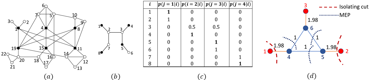
Minimum multiway $k$ cut for a non-planar graph: We now consider an instance of a $22$-node non planar graph, shown in Fig. 4a with unit edge-weights. In this example we consider a $6$-cut problem, whose set of terminals is specified as $S=\{1,4,8,11,15,19\}$. Our MEP algorithm results in a partition of the underlying graph, given by $\{1,2,3\}$, $\{4,5,6,7\}$, $\{8,9,10\}$, $\{11,12,13,14\}$, $\{15,16,17,18\}$ and $\{19,20,21,22\}$ with a cut value of 15; which is indeed optimal and can be easily verified. On the other hand, the isolating cut heuristic [4] for this randomly generated instance results in a cut solution with a value of 16. A similar observation is made on other randomly generated instances, where our algorithm results in optimal cut values (whenever verifiable). Moreover, the total run-time for the example in Fig. 4a for a naive implementation of the proposed approach in MATLAB is $<1$s on an Intel i7-4790 CPU @ 3.60 GHz.

Non-unique optimal cuts: In both the examples described above, the resulting optimal cuts are indeed unique. We now therefore consider a scenario with more than one permissible optimal cuts. Our algorithm identifies the multiplicity of optimal cuts, which is reflected in the final association matrix $\{p(j|i)\}$. Fig. 4b shows an example of a $8$-node graph with unit edge-weights and multiple permissible optimal $4$-cuts . Executing the proposed MEP-based algorithm results in the following association matrix. As shown in Fig. 4(c), node $3$ can be included in either $A_{2}$ or $A_{3}$ without affecting the value of the optimal cut, and therefore the association probabilities $p(j=2|i=3)=p(j=3|i=3)=0.5$. Assigning node $3$ to any of the two partitions still results in a feasible, yet optimal cut.

Comparison on challenging examples: Fig. 4d shows the performance of our MEP based approach on a toy-example (which can be generalized to any number of nodes. Here heuristic such as isolating cut [4], fails to identify an optimal cut for the simplest such scenario. In fact, it has been analytically shown that the isolating cut heuristic results can not give a solution within $2(1-1/k)$ of the optimal solution [4]. However, our algorithm finds the optimal multiway $k$-cut; thus achieving a cut which is impossible to obtain using the isolating cut method.

On Large Graphs: We also test our approach on large graphs with the number of nodes as large as $\sim 25000$ (corresponding to the size of the bounding box 150$\times$160 pixels). Figure 4 shows the results of our implementation of the interactive foreground-background segmentation (GrabCut [22]) using the proposed MEP approach. In GrabCut, an image is represented as a graph of pixels (nodes), where edge-weights capture differences in intensities between neighboring pixels. Users are required to demarcate the approximate foreground region using a bounding box as shown in Fig. 5. The proposed approach is then employed to segment and refine the foreground through successive minimization of s-t cuts of the resulting graphs. The implementation results in effective segmentation of foreground and background

Dynamic Graphs: Fig. 6 summarizes the steps of our algorithm. Fig. 7 illustrates the time-varying minimum multiway $2$-cut obtained on a weighted undirected dynamic graph using our proposed methodology. As stated in Section V the objective here is to find the time varying cuts $A_{1}$ and $A_{2}$ where the nodes $s_{1}$ and $s_{2}$ are the nodes $2$ and $4$ respectively. The edge-weight dynamics is given by $\dot{W}(t)=AW+BU$, which can be succinctly re-written as

Note that in the above system dynamics (VI), the edge $(1,2)$ is incapable of being influenced by any external control input. We simulate the dynamical system (24) for a total of $0.075$ seconds. Fig. 7(a) illustrates the minimum multiway $2$-cut given by the Algorithm 1 at the initial time $t_{0}$ where $A_{1}=\{1,2,3\}$, $A_{2}=\{4\}$. As time progresses the partitioning changes to $A_{1}=\{1,2\}$,$A_{2}=\{3,4\}$ in Fig. 7(b), $A_{1}=\{2\}$, $A_{2}=\{1,3,4\}$ in Fig. 7(c) and $A_{1}=\{1,2\}$, $A_{2}=\{3,4\}$ in Fig. 7(d).

In the frame-by-frame approach we first discretize the entire time interval of $0.075$ seconds with $\Delta t=0.01$ seconds and set $U(t)=0$ $\forall$ $t$, then Algorithm 1 is used to obtain the minimum multiway $2$-cut at each time instant. However this latter takes approximately $29$ times more computational time than required by our proposed method thereby making the frame-by-frame approach unscalable even for a very short duration of time.

In this paper, we formulate a statistical physics based algorithm for the minimum multiway $k$-cut problem on static as well as dynamic digraphs and present a convergence proof for the algorithm. The algorithm described in this paper is computationally efficient and has ability to avoid poor local minima through controlled randomness. We believe that a combination of good theoretical properties and experimental success of the proposed MEP-based algorithm makes it a suitable technique of choice for a wide variety of combinatorial optimization problems on graphs, such as, vertex coloring and finding independent sets.

References

- [1] S. Lowen, “Multiway cut,” 2011.
- [2] H. S. Stone, “Multiprocessor scheduling with the aid of network flow algorithms,” IEEE transactions on Software Engineering, no. 1, pp. 85–93, 1977.
- [3] P. L. Erdős and L. A. Székely, “On weighted multiway cuts in trees,” Mathematical programming, vol. 65, no. 1, pp. 93–105, 1994.
- [4] E. Dahlhaus, D. S. Johnson, C. H. Papadimitriou, P. D. Seymour, and M. Yannakakis, “The complexity of multiterminal cuts,” SIAM Journal on Computing, vol. 23, no. 4, pp. 864–894, 1994.
- [5] D. Marx, “A tight lower bound for planar multiway cut with fixed number of terminals,” in International Colloquium on Automata, Languages, and Programming. Springer, 2012, pp. 677–688.
- [6] A. Casteigts, P. Flocchini, W. Quattrociocchi, and N. Santoro, “Time-varying graphs and dynamic networks,” International Journal of Parallel, Emergent and Distributed Systems, vol. 27, no. 5, pp. 387–408, 2012.
- [7] J. Thomas, D. Seo, and L. Sael, “Review on graph clustering and subgraph similarity based analysis of neurological disorders,” International journal of molecular sciences, vol. 17, no. 6, p. 862, 2016.
- [8] E. T. Jaynes, “Information theory and statistical mechanics,” Physical review, vol. 106, no. 4, p. 620, 1957.
- [9] K. Rose, “Deterministic annealing for clustering, compression, classification, regression, and related optimization problems,” Proceedings of the IEEE, vol. 86, no. 11, pp. 2210–2239, 1998.
- [10] P. V. Gehler and O. Chapelle, “Deterministic annealing for multiple-instance learning.” in AIStats, 2007, pp. 123–130.
- [11] S. Mitra, R. Castellanos, and S. Joshi, “An adaptive deterministic annealing approach for medical image segmentation,” in Fuzzy Information Processing Society, 2000. NAFIPS. 19th International Conference of the North American. IEEE, 2000, pp. 82–84.
- [12] Y. Xu, S. M. Salapaka, and C. L. Beck, “Aggregation of graph models and markov chains by deterministic annealing,” Automatic Control, IEEE Transactions on, vol. 59, no. 10, pp. 2807–2812, 2014.
- [13] A. Rao, K. Rose, and A. Gersho, “Design of robust hmm speech recognizers using deterministic annealing,” in Automatic Speech Recognition and Understanding, 1997. Proceedings., 1997 IEEE Workshop on. IEEE, 1997, pp. 466–473.
- [14] M. Baranwal, B. Roehl, and S. M. Salapaka, “Multiple traveling salesmen and related problems: A maximum-entropy principle based approach,” in 2017 American Control Conference (ACC). IEEE, 2017, pp. 3944–3949.
- [15] Y. Xu, S. M. Salapaka, and C. L. Beck, “Clustering and coverage control for systems with acceleration-driven dynamics,” Automatic Control, IEEE Transactions on, vol. 59, no. 5, pp. 1342–1347, 2014.
- [16] G. Călinescu, H. Karloff, and Y. Rabani, “An improved approximation algorithm for multiway cut,” in Proceedings of the thirtieth annual ACM symposium on Theory of computing. ACM, 1998, pp. 48–52.
- [17] J. Naor and L. Zosin, “A 2-approximation algorithm for the directed multiway cut problem,” SIAM Journal on Computing, vol. 31, no. 2, pp. 477–482, 2001.
- [18] S. A. Gershgorin, “Uber die abgrenzung der eigenwerte einer matrix,” Proceedings of the Russian Academy of Sciences. Mathematical series, no. 6, pp. 749–754, 1931.
- [19] R. Sepulchre, M. Jankovic, and P. V. Kokotovic, Constructive nonlinear control. Springer Science & Business Media, 2012.
- [20] E. D. Sontag, “A lyapunov-like characterization of asymptotic controllability,” SIAM Journal on Control and Optimization, vol. 21, no. 3, pp. 462–471, 1983.
- [21] ——, “A universal construction of artstein’s theorem on nonlinear stabilization,” Systems & control letters, vol. 13, no. 2, pp. 117–123, 1989.
- [22] C. Rother, V. Kolmogorov, and A. Blake, “Grabcut: Interactive foreground extraction using iterated graph cuts,” in ACM transactions on graphics (TOG), vol. 23, no. 3. ACM, 2004, pp. 309–314.
- [23] T. H. Gronwall, “Note on the derivatives with respect to a parameter of the solutions of a system of differential equations,” Annals of Mathematics, pp. 292–296, 1919.