Time-Optimal Control of Collisional Gates in Ultracold Atomic Systems
Abstract
We use quantum optimal control to identify fast collision-based two-qubit gates in ultracold atoms. We show that a significant speed up can be achieved by optimizing the full gate instead of separately optimizing the merge-wait-separate sequence of the trapping potentials. Our optimal strategy does not rely on the atoms populating the lowest eigenstates of the merged potential, and it crucially includes accumulation of quantum phases before the potentials are fully merged. Our analyses transcend the particular trapping geometry, but to compare with previous works, we present systematic results for an optical lattice and find greatly improved gate durations and fidelities.
I Introduction
Optically trapped ultracold atomic systems have enjoyed impressive recent progress with regards to their preparation and control of both internal and external degrees of freedom Chu 2002; Bloch et al. 2008; Sherson et al. 2010; Weitenberg et al. 2011a. Especially, recent advances Kaufman et al. 2014; Wang et al. 2015; Kim et al. 2016; Endres et al. 2016; Barredo et al. 2016; Lee et al. 2016; Kumar et al. 2018; Barredo et al. 2018; Saskin et al. 2019; Norcia et al. 2018; Cooper et al. 2018 have augmented the viability of using the long coherence times of their spin internal degrees of freedoms for quantum computing Brennen et al. 1999; DiVincenzo 2000; Jaksch et al. 2000; Lukin et al. 2001; Daley et al. 2008; Negretti et al. 2011; Weitenberg et al. 2011b; Schneider and Saenz 2012; Jørgensen et al. 2014; Pagano et al. 2019. While single-qubit operations with fidelities above have been demonstrated in multiple experiments Xia et al. 2015; Wang et al. 2016, corresponding fidelities of two-qubit entangling operations are still subject of research Mandel et al. 2003; Anderlini et al. 2007; Wilk et al. 2010; Zhang et al. 2010; Isenhower et al. 2010; Maller et al. 2015; Kaufman et al. 2015; Jau et al. 2016; Levine et al. 2018. Entangling two-qubit gates can be mediated by long-range interactions such as dipole-dipole interactions between Rydberg atoms Jaksch et al. 2000; Browaeys et al. 2016; Saffman et al. 2010; Saffman 2016. Although the long-range nature of these interactions allows potentially fast operations, their use of highly excited atomic states make them vulnerable to enhanced coupling to the environment.
Short-range collisional (contact) interactions provide an alternative for neutral atom quantum gates Jaksch et al. 1999; Calarco et al. 2000; Anderlini et al. 2007; Hayes et al. 2007; Kaufman et al. 2015. Merging two initially separated atoms into a common trap initiates a collisional interaction depending on the exchange symmetry of the atomic wave function and hence of the spin state of the atoms. After a duration determined by the interaction strength in the merged state, the atoms are spatially separated, and under appropriate conditions, the simple three-stage merge-wait-separate sequence illustrated in Fig. 1 realizes the entangling gate.
The short-range character of the collisions ensures that only the desired qubits participate in the operation, decreasing the detrimental coupling to other qubits and to the environment. Relying on collisional interaction imposes strong requirements for the precision with which the spatial degree of freedom of the atoms must be controlled. Current experimental control protocols to perform this entangling gate are thus adiabatic in nature, but this severely limits the total number of gate operations before decoherence effects become significant Anderlini et al. 2007; Kaufman et al. 2015.

Finding fast, complex control protocols is a task well-suited for quantum optimal control. Previous works De Chiara et al. 2008; Mundt and Tannor 2009 have thus reduced the duration of the merging stage in optical geometries by orders of magnitude compared to adiabatic solutions. However, the current best results for the merging stage have thus far not crossed the 0.99 threshold. This is especially detrimental since even slight merging errors also reduce the quality of subsequent waiting and separation stages. To our knowledge, no optimization of the full gate has been carried out.
In this paper, we discuss how the gate relies on the evolution of a relative phase between singlet and triplet spin state components, and why the partial accumulation of this phase already during the merging stage is a challenge for the optimization of stagewise protocols. We develop means to solve this challenge, and we proceed to show that a protocol without dedicated merge-wait-separate stages yields faster performance and 0.99 fidelity for the full operation with ultracold 87Rb atoms. We stress that our considerations of the accumulated relative phase and the full gate optimization are independent of the specific physical problem geometry, atomic species as well as model dimensionality.
The paper is organized as follows. In Sec. II we present the trapping geometry under consideration for the operation. In Sec. III we present the theory for implementing the gate in ultracold atoms. The two-particle Hamiltonian is introduced and general properties of the allowed states are discussed. Initially, we use symmetrized product states to construct the computational basis states. Using these states, we describe the important accumulated relative phase during the merging sequence. In our numerical optimization, we do not rely on the independent particle approximation but propagate genuine two-particle wave functions for the interacting atoms. In Sec. IV we discuss the difference between the staged merge-wait-separate approach and the full gate approach in terms of optimal trajectories in Hilbert space. In Sec. V we present and discuss the results. In Sec. VI we summarize the main conclusions of the paper.
II Trapping geometry
A necessary feature of any candidate geometry for the collisional operation is the possibility to bring two atoms from a separated configuration into contact by, for example, merging them in a common trap as illustrated in Fig. 1. We consider the implementation with an optical lattice Anderlini et al. 2006; Anderlini et al. 2007 that has been loaded with a Mott state of unit filling and where the atoms at every other site have been prepared with opposite spin states. An analysis presented in Appendix A justifies a 1D description with the potential
| (1) |
Here provides the overall lattice depth, while and adjust the height and tilt of adjacent wells. By controlling , pairs of adjacent wells are transformed from a double-well into a single-well configuration as illustrated in Fig. 2. In an independent-particle picture, the atom in the ground state of the Left (Right) well is transferred to the first excited (ground) state of the merged well, .
III gate with cold Atoms
The gate is concerned with the qubit, i.e., spin degrees of freedom of the atoms, and its simplest implementation is through the three-stage merge-wait-separate sequence in Fig. 1. In this section, we recall the theory behind this procedure.
The system is described by the effective Hamiltonian
| (2) |
Here, are the coordinates of the two atoms, is the single-particle Hamiltonian with trapping potential . The form of the interaction term and the value of the coupling strength are discussed in Appendix A.
We use identical bosonic atoms and the full two-particle state can thus be expanded on symmetric states of the form
| (3) | ||||||
| (4) | ||||||
with the symmetric () spin triplet and anti-symmetric spin singlet states
| (5) |
and symmetric () and anti-symmetric spatial states , where proper normalization is implied in the remainder of the paper.
The Hamiltonian (2) is independent of the spin degrees of freedom and cannot induce transitions between states of different total spin. The interaction term only acts on the component since by construction. This introduces an energy difference between the otherwise degenerate singlet and the triplet state vector components. This energy difference is the main mechanism behind the gate.
III.1 Symmetrized Product States
To illustrate the dynamics leading to the operation we consider an approximate analysis with symmetrized product states, but we emphasize that our numerical optimization is carried out with the full two-particle interaction dynamics.
We associate the qubits with the spins of atoms occupying definite spatial states. If and denote such single-particle eigenstates of , spatially symmetrized product states
| (6) |
are approximate eigenstates of with energies
| (7) | ||||
| (8) |
where and are single-particle energies and
| (9) |
The energy difference between clearly depends on the spatial overlap of the two atoms and the collisional coupling strength.
Using (6) in (3)-(4), we define symmetrized computational basis states for the operation:
| (10) | ||||||
| (11) | ||||||
| (12) | ||||||
| (13) |
We see in the two first lines that the relative phase between the triplet and singlet components is essential to determine how the spins are correlated with the spatial states of the atoms. The two last lines represent states that are unaffected by the operation and acquire only the same phase factor as the components in the two first lines.
We define the gate in the states (10)-(13) as
| (14) | ||||
| (15) | ||||
| (16) | ||||
| (17) |
If the spins are initially in opposite states, the operation yields an entangled state. If the spins are initially equal a phase is applied. In the following, we focus on the mapping (14) and study the approximate system dynamics to find the necessary conditions for implementing the gate.
Time Evolution in Static Trap
If and are single-particle eigenstates of , the time evolution of is approximately given by
| (18) | ||||
| (19) |
where we disregard global phases as the dynamics of the system and the spin distribution on the atoms is fully described by the relative phase between the state components. After the duration () the spins are fully swapped while the interaction for half of this duration () implements the desired gate as illustrated in Fig. 4.
The spin swapping rate depends only on the interaction energy Eq. (9), which remains constant throughout the evolution in a static trap. To obtain a finite the atoms must therefore be sufficiently overlapping. This condition is satisfied in the merged configuration, but clearly not in the initial configuration – see Fig. 2(a) and (c).
Time Evolution in Adiabatically Transformed Trap
Suppose the trapping potential is transformed adiabatically with respect to the single-particle states such that and follow instantaneous eigenstates of . Then the time evolution given by Eq. (19) remains valid with . The spin swapping rate is now time-dependent and becomes non-zero as the atoms begin to overlap.
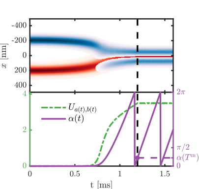
As a consequence, the phase accumulated during the merging is in general , which reduces the waiting stage duration needed to obtain the entangled state. This is clearly seen in Fig. 4 if we let ; the phase acquired during merging already brought the state closer to . An additional will be acquired during the separation stage. Assuming for simplicity , the duration is reduced to where the factor 2 accounts for both the merging and separation stage. Labeling explicitly the merging duration by , the total duration of the full gate operation using the merge-wait-separate sequence is then .
This sequence explicitly implements the mapping of a single basis state (14). Fortunately, such sequence also simultaneously realizes the remaining mappings. The mapping (15) simply corresponds to starting at from where the phase accumulation proceeds identically to above. For the mappings (16)-(17), note that (14) implies correct, simultaneous preparation of the individual triplet and singlet components since there is no coupling between states of different symmetry. Thus, these mappings are also guaranteed to be realized. We note at this point that the converse is not necessarily true: a sequence implementing mappings (16)-(17) does not guarantee the mappings (14)-(15) since the singlet component is absent.
To summarize the ideas developed in this section, we show a numerical example of the accumulated phase to illustrate qualitative features in Fig. 4. Here, the system from Fig. 2 is adiabatically merged and followed by a holding time in the static final potential 11 1 Visit https://www.quatomic.com/quatomic_publications/ for animations of the single-particle densities.. The single-particle states are propagated independently with the interaction only affecting the relative phase and not the spatial distribution, which is the approximation made in Eq. (18). At each point in time we construct and calculate the corresponding . As the atoms begin to overlap the relative phase accumulates resulting in . Following the merge, the state is obtained after a short, static holding time of about . If instead the atoms were immediately separated, the state would be obtained since .
The adiabatic transfer thus ensures a high-fidelity implementation of the gate since we are guaranteed to stay within the superposition of just one singlet and triplet state Eq. (18). However, for the purposes of quantum computation we also need the implementation to be fast. The speed up is achieved by exploiting the interference effects of many intermediately populated excited states. To enable the engineering of these very complicated diabatic transfers we turn to quantum optimal control. Before doing so, we close this section by replacing the symmetrized product states with the true two-particle eigenstates.
III.2 Two-Particle Eigenstates
The analysis of the dynamics in the previous section approximated the symmetrized product states Eq. (6) to be eigenstates of where and were eigenstates of . In the limit of vanishing interactions (no spatial overlap or zero coupling) this approximation is exact. This allows us to relate to the true spatial two-particle eigenstates (annotated with ) in the following way:
| (20) | ||||
| (21) |
where in this context implies vanishing interactions. Only the triplet state is affected by the interaction as the system can lower its energy by depleting the diagonal . This notation is very convenient since we retain reference to the intuitive independent-particle picture. In particular, the analysis following Eq. (6) of the previous section is still valid upon annotating all states and energies with ’’. The approximation made in Eq. (18) consisted in ignoring the small interaction matrix elements between different triplet states (other off-diagonal elements vanish identically) such that the symmetrized product states were approximate eigenstates of the full Hamiltonian. In using the true eigenstates , the results are exact.
It is also possible to describe the dynamics in a static potential with an effective spin Hamiltonian even though the spin swapping is purely due to spatial effects (extension to the adiabatic case is straightforward). This is also known as the exchange interaction. Here are spin operators and is the exchange energy. See Appendix C for a brief derivation of this result.
IV Quantum Optimal Control of in Ultracold Atoms
In Sec. III we showed that the desired operation can be implemented based on a single basis state mapping . Formulating this as a state transfer control problem, the initial- and target states for the full gate are
| (22) | ||||
| (23) |
By writing the states in terms of singlet and triplet components we emphasize the goal of ultimately establishing the correct relative phase in the separated configuration by letting the atoms collide. See Appendix B for a description of methods and problem parameters.
A simplified approach to solving the control problem is to use the merge-wait-separate sequence. The problem can then be reduced to optimizing just the merging stage as the associated optimal controls can be extended to implement the whole sequence: the waiting stage duration is determined by the relative phase acquired during the optimized merging stage, whereas the separation stage is carried out by propagating along the time-inverted optimized merging control. A suitable target state for the merging sub-problem is
| (24) |
The merging sub-problem thus consists in realizing . This target state is not stationary and will exhibit two-level beating dynamics if the transfer is successful. Note the inclusion of a target relative phase . This is because is monotonically increasing due to . If the target phase is excluded (), then, in an independent-particle picture, the optimizer will try to minimize the time-integrated overlap between the atomic states during the transfer. This is contradictory to the overall goal of the merging, which is exactly to overlap the atoms to enable the spin swapping. The total accumulated phase is not crucial to the overall operation since one may simply adjust the duration of the waiting stage. It follows that any final superposition of is acceptable as long as . In fact, a non-zero phase within this range is beneficial as it speeds up the overall gate operation, see Fig. 4. However, the standard figure of merit for the state transfer quality is the fidelity
| (25) |
which for the merging sub-problem, , depends on the chosen target phase. In this case a more appropriate measure of the transfer quality insensitive to the relative phase is the total population in :
| (26) |
where only when . Thus, optimizing would alleviate the constraint on the relative phase. Instead of doing this, we simply use as a stopping condition and optimize with an appropriate target phase such that . For the durations under consideration, numerical investigations suggest typical values of . This is well below . We find a suitable target phase to be . The optimization could be improved by making an appropriate cost functional replacement and deriving the resulting optimality system.
Previous works De Chiara et al. 2008; Mundt and Tannor 2009 considered only the merging sub-problem and did not include the singlet component in initial nor target state, using only the triplet component. This corresponds to realizing the mappings (16)-(17), which as previously mentioned does not guarantee simultaneous implementation of the remaining mappings (14)-(15) but may still be considered an approximation. Additionally, ignoring the singlet component reduces the problem difficulty since the optimization no longer has to achieve a relative phase.
The merit of solving the full control problem by reducing it to the merging sub-problem is its conceptual simplicity. From a numerical point of view, it also typically involves a reduced interval of time integration. This is substantial due to the low time resolution required to faithfully simulate the interaction -function. Nevertheless, there are several drawbacks to this approach. Firstly, optimizing towards is an artificial and unnecessarily strict condition. It can be understood as forcing the optimal state trajectories to pass through a particular intermediate point (or small volume in case of ) in Hilbert space as illustrated by the upper trajectories in Fig. 5. Secondly, extending optimal controls to implement the complete merge-wait-separate sequence is predicated on idealized unit fidelity transfers wrt. . Even 0.99 fidelity solutions will have their errors exacerbated throughout the waiting- and separation stages, causing alterations to the state trajectory away from , which is the state we are ultimately interested in obtaining. The lower trajectories in Fig. 5 corresponds to optimizing the full problem directly and is not required to pass through any particular intermediate state. The control problem is not broken up into distinct stages and becomes much less restrictive.
In this work we combine the two approaches. We first optimize towards in the merging sub-problem. We subsequently extend the corresponding optimized controls to implement the full gate. These extended controls are then used as seeds for the optimization towards in the full gate problem. This methodology allows a fair comparison of the two approaches.
V Results
In this section we present optimization results. A solution is considered optimal if it exceeds in the sub-merging problem or in the full problem.
Fig. 7 shows optimization results for the merging sub-problem. A total of 2544 seeds were optimized with between 100 and 250 seeds per duration. The red dots show for the best controls obtained for each . We find the upper bound for the quantum speed limit to be (see Appendix B.2 for the corresponding time-optimal control). Compared to previous results of 0.97 fidelity De Chiara et al. 2008; Mundt and Tannor 2009 (which also uses more approximations), this is still a factor reduction in duration. Using instead 0.97 as the fidelity threshold the reduction is . The blue translucent dots show for all optimized controls, where the translucency indicates the distribution density. From the translucency we see the average quality of the optimized controls increases with duration as the problem becomes easier (the seeming increase in low-fidelity solutions for the last three durations is due to an increased overall number of seeds). Nevertheless, the best obtained fidelities plateaus around 0.988 over a rather long interval. As discussed previously, the full gate can be realized by extending the merging optimized controls. This is shown for the time-optimal controls at in Fig. 8 where instantaneous fidelities with various states are plotted as a function of time. We also plot the corresponding independently propagated single-particle wave functions Note1. The initial state is transferred into the merged trap in time with and acquires a phase of during merging. The waiting stage with two-level dynamics lasts for and nearly enters the entangled state. The controlled termination of the exchange interaction ensures that the remaining phase is acquired in the separation stage such that the final state is approximately with fidelity . The total gate time is . We note that the process is fundamentally limited by the rate at which entanglement can be generated. To provide a sense of scale, prepared in the merged configuration would achieve in , which illustrates that there is still room for improvement.
The top row of table 1 summarizes several figures of merit for various states when propagated along the time-optimal control. The superscripts m and f indicate if the quantity is measured at the merging or full gate duration, respectively. Here, and are the single-particle fidelities corresponding to the merging transfer , and are the single-particle fidelities corresponding to the transfer when extending the merging optimized control to the full gate, are the merging fidelities when including only the triplet () or singlet () component in the initial and target state, and is the merging fidelity if the target phase is excluded.
The high single-particle fidelities and indicate that the imperfection in is mainly due to the interaction affecting the triplet and singlet components differently. A supporting observation is that while . This shows that relative phase acquired during the merging is a small but significant effect for producing high quality solutions. Additionally, from comparing and we explicitly see that fidelity is not the best figure of merit for the merging sub-problem, but using it for optimization is still good enough when using as a stopping condition.
In Fig. 7 we show optimization results for the full gate problem, using optimized merging controls as seeds. 2323 seeds were optimized while the remaining 221 were left out due to . The red dots show for the monotonically best and optimal solutions, as there are now many unique durations (depending on ). We find the upper bound for the quantum speed limit for the full gate to be (see Appendix B.2 for the corresponding time-optimal control). This is faster than for merging alone from Refs. De Chiara et al. 2008; Mundt and Tannor 2009 and faster than using the extended optimal merging solution. Additionally, the sub-optimal plateau is now completely absent and we find an increase in optimal solutions by two orders of magnitude. The blue dots show for all solutions.
Fig. 9 shows fidelities and independent single-particle densities when propagated along the time-optimal control at Note1. Although there are no explicit distinct stages after optimizing, remnants of the seed’s merge-wait-separate sequence (durations marked for reference) is still visible. For example, the time-optimal control as well as single-particle densities remain essentially symmetric around the . The bottom row of table 1 summarizes figures of merit for various states. The situation is quite different from Fig. 8 as the Hilbert space state trajectory is never close to passing through (or equivalently in the independent-particle picture). Nevertheless, the atomic overlap and interaction around remains appreciable as the motional excitations allows for synchronized in-phase oscillations. Finally, is prepared with at the end duration. Interestingly, the seed that optimized to the time-optimal control initially had only at . These numerical observations evidence that the restrictions imposed by the merge-wait-separate approach are indeed unnecessarily restrictive.
The plateau in Fig. 7 suggests the existence of optimal merging controls at even lower durations, which could be uncovered by increasing the number of seeds and more elaborate seeding strategies. However, the fact remains that such solutions can practically always be further improved by subsequently optimizing the full gate. It would be more interesting to investigate the full gate with completely independently generated seeds as the current optimal solutions inherits at least partially the merge-wait-separate stages. Additionally, the single-particle densities seem to have low velocities near the beginning and the end of the transfer. One can imagine rapidly transforming into the single-well configuration: both atoms are then subject to a large initial acceleration towards each other and will evolve without changing their shape appreciably as they closely resemble coherent states in a harmonic oscillator. As the atoms approach each other, suppose that the atoms could be decelerated to low momenta such that they oscillate out of phase with low amplitudes around the trap center. This would allow rapid entanglement since identical shapes maximize the interaction Eq. (9). If the necessary relative phase is acquired within a little less than a single or few oscillation periods, each atom will already have correctly directed opposite momenta at the onset of separation. This is different from the case of in-phase oscillations in Fig. 9 where both atoms must be more delicately provided opposite accelerations to correctly separate them. A similar scheme to the above is presented in Refs. Calarco et al. 2000; Treutlein et al. 2006 for another type of collisional gate. Whether such strategies are indeed effective in producing better solutions can only be verified by further numerical investigations and is left for future work.
VI Conclusions
We have presented and discussed in great detail the theory behind collisional gate implementation in cold atoms. Prime among these considerations is proper accounting of the relative phase acquired during merging. Additionally, we argued that optimizing the full gate directly instead of the staged merge-wait-separate sequence is favorable both in terms of final fidelity and optimal trajectories in Hilbert space. The relative phase and the full gate optimization allow separate reductions of the overall gate duration. Both concepts transcend any particular geometry, atomic species, and model dimensionality. They may thus be relevant in future work.
We then verified these claims in an optical lattice geometry. For the merging sub-problem, we find at which is an improvement over previous similar results of at . Nevertheless, a sub-optimal plateau of solutions indicate that the merging sub-problem is hard to solve and even in the best case the corresponding full gate fidelity is sub-optimal at in . By instead using the merging optimized solutions as seeds for the full gate problem the sub-optimal plateau is eliminated while also yielding a significantly increased number of optimal solutions with durations as low as .
VII Acknowledgements
This work was funded by the European Research Council, John Templeton Foundation, and the Carlsberg Foundation. The numerical results presented in this work were obtained at the Centre for Scientific Computing, Aarhus http://phys.au.dk/forskning/cscaa/.
| Single-particle | Two-particle | |||||||||||
|---|---|---|---|---|---|---|---|---|---|---|---|---|
| Merging optimized | 0.994 | 0.997 | 0.992 | 0.992 | 0.992 | 0.988 | 0.950 | 0.9886 | 0.990 | 0.983 | ||
| Full gate optimized | 0.540 | 0.868 | 0.997 | 0.996 | 0.570 | 0.473 | 0.498 | 0.519 | 0.522 | 0.990 | ||


Appendix A Effective 1D Description
Denoting by () the spatial and spin degrees of freedom for the ’th particle, the full 3D Hamiltonian describing two interacting spin- particles is
| (27) |
where is the sum of kinetic energy operators over all particle coordinates, is the single-particle trapping potential, and is the interaction potential. Exactly solving the associated equations of motion for is computationally expensive even for very crude spatial discretizations. For this reason, it is desirable to describe the approximate dynamics in an effective 1D model in which the spin states are treated implicitly. This can be done under the assumption that motion in the remaining spatial axes are frozen out and the Hamiltonian is void of spin terms. In this approximation, the variables separate into the product form
| (28) |
where is the only part of the wave function with a time evolution different from a trivial phase. The motional wave functions in the and -directions remain in their respective ground state at all times, and the spin wave function remains unchanged. We can then restrict our attention to the non-trivial part of the state and drop the superscript as we have done throughout the main text. We briefly discuss the steps to obtain (28) in the following.
The spin degrees of freedom separate exactly since there is no spin dependence in Eq. (27). The spatial coordinates cannot be separated immediately because couples them all. To proceed, we define where and approximate the potential in and to be locally harmonic. This allows an approximate 1D description Olshanii 1998 of the inter-particle coupling
| (29) | ||||
| (30) |
Importantly, the local harmonic frequency () in the ()-direction may become position dependent in . To calculate these frequencies is Taylor expanded to second order around the point . Assuming that is a minimum in and one obtains
| (31) |
Comparing the two expressions we obtain the frequencies . The full 3D potential for the optical lattice Anderlini et al. 2006; Anderlini et al. 2007; De Chiara et al. 2008 and corresponding frequencies are
| (32) | ||||
| (33) |
As does not depend on , the -degrees of freedom separate exactly in these approximations. Excitations along this axis can always be suppressed by choosing the independent trap depth to generate sufficiently large vibrational frequencies with associated energy spacings. On the contrary, the separation of the and coordinates is only approximate since . Our calculations of the full 2D single-particle spectrum show that the trapping along is only slightly weaker than along , since is common to both axes. It is therefore much harder to suppress excitations along than . Errors induced by the approximate potential separability of and is the main limitation of the model, since this coupling is much larger than the inter-particle coupling . The quality of the approximation (28) can thus be assessed on the independent-particle level. In Fig. 12 we propagate the particle starting in the left ground state over the time-optimal control at and compute the 1D and 2D instantaneous fidelities with the initial state. Their difference corresponds roughly to the leakage out of the ground state in the -direction induced by the non-separability of the potential. The effects are less pronounced for the particle starting in the right ground state. We have done the same for the optimized control presented in Fig. 7 from Ref. De Chiara et al. 2008 and find similar results.
Appendix B Methods
B.1 Numerics
The simulations and optimization results presented in this paper are produced with the QEngine Sørensen et al. 2019, our recent C++ software package for quantum optimal control.
The singlet and triplet states are obtained through numerical diagonalization in the discrete -representation with uniform grid-spacing. The 5-diagonal approximation is used for the Laplacian. Propagation is performed using split-step FFT, which is fastest if the number of spatial grid points are integer powers of 2, e.g. . We employ a state absorptive imaginary potential near the grid borders to minimize the effects of the periodic boundary conditions induced by the split-step FFT method. The in the interaction potential necessitates a very high degree of temporal resolution to reliably produce the correct dynamics. Numerical experiments show that is a good value for the simulation. At this very high temporal resolution the spatial resolution is found to be stable over a surprisingly broad range. Propagating thousands of different controls, the mean and standard deviation measured between fidelities produced with and is roughly . Increasing has almost no effect. However, even at this relatively modest the time discretization still requires steps to reach the durations of interest and as a result performing optimization with these parameters is very slow. To significantly speed up the optimization by several orders of magnitude we instead use increasingly finer grids. A grid is defined by the tuple . For the merging sub-problem, we optimize on the grids sequentially . The control is interpolated linearly to the new when moving between the grids. This allows performing a large scale multistarting optimization at a broad range of on the approximate time scale of several days. Due to memory issues we only optimize the full gate on the grids and then simply evaluate on the final grid when reporting results.
B.2 Optimal Control
To solve the state transfer problem , we use the gradient based grape algorithm with the l-bfgs search direction to minimize the cost functional
by iteratively improving the set of control fields (protocols) . The gradient is calculated using the adjoint method by introducing an additional Lagrange multiplier term.
Minimizing corresponds to maximizing the fidelity where is the time evolution operator.
adds preference to smoother controls with strength and adds preference to controls within specified parameter boundaries with strength . In the latter context, is a function that is zero when the boundaries are respected and parabolic when exceeded Sørensen et al. 2019.
As mentioned in the main text, a more appropriate measure of the transfer quality for the merging sub-problem is the total population . This could be directly accommodated in the cost functional by replacing with
which is minimized when is fully and equally distributed in the states independent of relative phase, see Eq. (24). This replacement requires calculating new Gâteaux derivatives to obtain a new optimality system Sørensen et al. 2019.
Instead of formally doing this we simply use as a stopping condition.
We simulate rubidium atoms with mass and assume a state independent scattering length Kaufman et al. 2014; Julienne et al. 1997 where is the Bohr radius. We restrict our attention to a single unit cell of the lattice defined within where Anderlini et al. 2007 is the lattice site separation for the initial configuration Fig. 2(a). We pad the boundaries slightly such that for numerical reasons: in the boundary region a constant is used to stabilize the diagonalization. We have verified that the wave function does not enter this non-physical region when propagated along the optimized controls. The independent lattice in the -direction has strength Anderlini et al. 2007.
The control parameters of the potential Eq. (1) are rescaled as with values
The unscaled initial and final control values for the merging sub-problem (, , ) are chosen to allow comparison with results in Ref. De Chiara et al. 2008. Similar values are used in Ref. Mundt and Tannor 2009. Neither paper discuss rescaling. For the full gate problem .
Fig. 10 shows a few select two-particle spatial states. For the separated configuration Fig. 2(a), (singly occupied wells) are degenerate, while the interaction increases the energy of (doubly occupied wells) by as was also reported in Ref. De Chiara et al. 2008. Note that the numerical initial state and target state are not immediately symmetric, but are still physically correct since the appropriate spin degree of freedom is implicitly included.
We include a regularization term with for all controls and a boundary term to constrain with such that the adjacent lattice unit cells do not mix and remains reasonably lower than (see Appendix A). Optimization seeds for merging are generated by perturbing a reference control with random sines of increasing harmonic frequency with random weighting and overall normalization. The reference control was heuristically chosen such that the seed cost is on average decreased. As discussed in the main text, the optimized merging controls are used as seeds for the full gate optimization. In both cases we optimize the seeds until they exceed the figure of merit threshold, converge to a local minimum, or exceed a wall time limit of 7 days. Figs. 12 and 13 shows the time-optimal controls for the merging and full gate problems, respectively Note1.

Appendix C Spin Exchange Hamiltonian
The collisional effects modeled by Eq. (2) is purely spatial which allowed us to treat the spin states implicitly. However, if the trapping geometry is static and the spatial state is a superposition on the form we can describe the dynamics with an effective spin Hamiltonian where are spin operators and is the exchange energy. The matrix representation of in the standard computational basis is
| (34) |
where are standard unit vectors. Clearly the computational basis states are not eigenstates of unless . Diagonalizing of Eq. (34) yields energies and corresponding states
with three degenerate states corresponding to . The states are exactly the spin singlet and triplet spin states with an energy difference of , while and are the remaining triplet spin states with a non-zero net spin. In this effective spin model, it is the spatial degree of freedom that is treated implicitly. Thus, the time evolution for the initially prepared state is
where and we ignored a global phase. This model exactly reproduces the dynamics from Eq. (19).
References
- Chu (2002) S. Chu, Nature 416, 206 (2002).
- Bloch et al. (2008) I. Bloch, J. Dalibard, and W. Zwerger, Reviews of modern physics 80, 885 (2008).
- Sherson et al. (2010) J. F. Sherson, C. Weitenberg, M. Endres, M. Cheneau, I. Bloch, and S. Kuhr, Nature 467, 68 (2010).
- Weitenberg et al. (2011a) C. Weitenberg, M. Endres, J. F. Sherson, M. Cheneau, P. Schauß, T. Fukuhara, I. Bloch, and S. Kuhr, Nature 471, 319 (2011a).
- Kaufman et al. (2014) A. Kaufman, B. Lester, C. Reynolds, M. Wall, M. Foss-Feig, K. Hazzard, A. Rey, and C. Regal, Science 345, 306 (2014).
- Wang et al. (2015) Y. Wang, X. Zhang, T. A. Corcovilos, A. Kumar, and D. S. Weiss, Physical review letters 115, 043003 (2015).
- Kim et al. (2016) H. Kim, W. Lee, H.-g. Lee, H. Jo, Y. Song, and J. Ahn, Nature communications 7, 13317 (2016).
- Endres et al. (2016) M. Endres, H. Bernien, A. Keesling, H. Levine, E. R. Anschuetz, A. Krajenbrink, C. Senko, V. Vuletic, M. Greiner, and M. D. Lukin, Science 354, 1024 (2016).
- Barredo et al. (2016) D. Barredo, S. De Léséleuc, V. Lienhard, T. Lahaye, and A. Browaeys, Science 354, 1021 (2016).
- Lee et al. (2016) W. Lee, H. Kim, and J. Ahn, Optics express 24, 9816 (2016).
- Kumar et al. (2018) A. Kumar, T.-Y. Wu, F. Giraldo, and D. S. Weiss, Nature 561, 83 (2018).
- Barredo et al. (2018) D. Barredo, V. Lienhard, S. de Léséleuc, T. Lahaye, and A. Browaeys, Nature 561, 79 (2018).
- Saskin et al. (2019) S. Saskin, J. Wilson, B. Grinkemeyer, and J. D. Thompson, Physical review letters 122, 143002 (2019).
- Norcia et al. (2018) M. Norcia, A. Young, and A. Kaufman, Physical Review X 8, 041054 (2018).
- Cooper et al. (2018) A. Cooper, J. P. Covey, I. S. Madjarov, S. G. Porsev, M. S. Safronova, and M. Endres, Physical Review X 8, 041055 (2018).
- Brennen et al. (1999) G. K. Brennen, C. M. Caves, P. S. Jessen, and I. H. Deutsch, Physical Review Letters 82, 1060 (1999).
- DiVincenzo (2000) D. P. DiVincenzo, Fortschritte der Physik: Progress of Physics 48, 771 (2000).
- Jaksch et al. (2000) D. Jaksch, J. I. Cirac, P. Zoller, S. L. Rolston, R. Côté, and M. D. Lukin, Physical Review Letters 85, 2208 (2000).
- Lukin et al. (2001) M. Lukin, M. Fleischhauer, R. Cote, L. Duan, D. Jaksch, J. Cirac, and P. Zoller, Physical review letters 87, 037901 (2001).
- Daley et al. (2008) A. J. Daley, M. M. Boyd, J. Ye, and P. Zoller, Physical review letters 101, 170504 (2008).
- Negretti et al. (2011) A. Negretti, P. Treutlein, and T. Calarco, Quantum information processing 10, 721 (2011).
- Weitenberg et al. (2011b) C. Weitenberg, S. Kuhr, K. Mølmer, and J. F. Sherson, Physical Review A 84, 032322 (2011b).
- Schneider and Saenz (2012) P.-I. Schneider and A. Saenz, Physical Review A 85, 050304 (2012).
- Jørgensen et al. (2014) N. B. Jørgensen, M. G. Bason, and J. F. Sherson, Phys. Rev. A 89, 032306 (2014).
- Pagano et al. (2019) G. Pagano, F. Scazza, and M. Foss-Feig, Advanced Quantum Technologies 2, 1800067 (2019).
- Xia et al. (2015) T. Xia, M. Lichtman, K. Maller, A. Carr, M. Piotrowicz, L. Isenhower, and M. Saffman, Physical review letters 114, 100503 (2015).
- Wang et al. (2016) Y. Wang, A. Kumar, T.-Y. Wu, and D. S. Weiss, Science 352, 1562 (2016).
- Mandel et al. (2003) O. Mandel, M. Greiner, A. Widera, T. Rom, T. W. Hänsch, and I. Bloch, Nature 425, 937 (2003).
- Anderlini et al. (2007) M. Anderlini, P. J. Lee, B. L. Brown, J. Sebby-Strabley, W. D. Phillips, and J. Porto, Nature 448, 452 (2007).
- Wilk et al. (2010) T. Wilk, A. Gaëtan, C. Evellin, J. Wolters, Y. Miroshnychenko, P. Grangier, and A. Browaeys, Physical Review Letters 104, 010502 (2010).
- Zhang et al. (2010) X. Zhang, L. Isenhower, A. Gill, T. Walker, and M. Saffman, Physical Review A 82, 030306 (2010).
- Isenhower et al. (2010) L. Isenhower, E. Urban, X. Zhang, A. Gill, T. Henage, T. A. Johnson, T. Walker, and M. Saffman, Physical review letters 104, 010503 (2010).
- Maller et al. (2015) K. Maller, M. Lichtman, T. Xia, Y. Sun, M. Piotrowicz, A. Carr, L. Isenhower, and M. Saffman, Physical Review A 92, 022336 (2015).
- Kaufman et al. (2015) A. Kaufman, B. Lester, M. Foss-Feig, M. Wall, A. Rey, and C. Regal, Nature 527, 208 (2015).
- Jau et al. (2016) Y.-Y. Jau, A. Hankin, T. Keating, I. Deutsch, and G. Biedermann, Nature Physics 12, 71 (2016).
- Levine et al. (2018) H. Levine, A. Keesling, A. Omran, H. Bernien, S. Schwartz, A. S. Zibrov, M. Endres, M. Greiner, V. Vuletić, and M. D. Lukin, Physical review letters 121, 123603 (2018).
- Browaeys et al. (2016) A. Browaeys, D. Barredo, and T. Lahaye, Journal of Physics B: Atomic, Molecular and Optical Physics 49, 152001 (2016).
- Saffman et al. (2010) M. Saffman, T. G. Walker, and K. Mølmer, Reviews of Modern Physics 82, 2313 (2010).
- Saffman (2016) M. Saffman, Journal of Physics B: Atomic, Molecular and Optical Physics 49, 202001 (2016).
- Jaksch et al. (1999) D. Jaksch, H.-J. Briegel, J. Cirac, C. Gardiner, and P. Zoller, Physical Review Letters 82, 1975 (1999).
- Calarco et al. (2000) T. Calarco, E. Hinds, D. Jaksch, J. Schmiedmayer, J. Cirac, and P. Zoller, Physical Review A 61, 022304 (2000).
- Hayes et al. (2007) D. Hayes, P. S. Julienne, and I. H. Deutsch, Phys. Rev. Lett. 98, 070501 (2007).
- De Chiara et al. (2008) G. De Chiara, T. Calarco, M. Anderlini, S. Montangero, P. Lee, B. Brown, W. Phillips, and J. Porto, Physical Review A 77, 052333 (2008).
- Mundt and Tannor (2009) M. Mundt and D. J. Tannor, New Journal of Physics 11, 105038 (2009).
- Anderlini et al. (2006) M. Anderlini, J. Sebby-Strabley, J. Kruse, J. V. Porto, and W. D. Phillips, Journal of Physics B: Atomic, Molecular and Optical Physics 39, S199 (2006).
- (46) Note1, visit https://www.quatomic.com/quatomic_publications/ for animations of the single-particle densities.
- Treutlein et al. (2006) P. Treutlein, T. W. Hänsch, J. Reichel, A. Negretti, M. A. Cirone, and T. Calarco, Physical Review A 74, 022312 (2006).
- Olshanii (1998) M. Olshanii, Physical Review Letters 81, 938 (1998).
- Sørensen et al. (2019) J. Sørensen, J. Jensen, T. Heinzel, and J. Sherson, Computer Physics Communications 243, 135 (2019).
- Julienne et al. (1997) P. S. Julienne, F. Mies, E. Tiesinga, and C. J. Williams, Physical review letters 78, 1880 (1997).