跳到论文正文
W Papers独立论文阅读器 arXiv:1907.08414 论文正文 计算阅读时间 · 0%
引用这篇论文根据当前论文元数据生成,正式投稿前建议核对。


License: arXiv.org perpetual non-exclusive license
arXiv:1907.08414v3 [stat.ME] 11 Feb 2023

Reluctant Interaction Modeling

Guo Yu Thanks: Department of Statistics and Applied Probability, University of California Santa Barbara, Santa Barbara, CA 93110, guoyu@ucsb.edu    Jacob Bien Thanks: Data Sciences and Operations, Marshall School of Business, University of Southern California, Los Angeles, CA 90089, jbien@usc.edu    Ryan Tibshirani Thanks: Department of Statistics, University of California Berkeley, Berkeley, CA 94720, ryantibs@berkeley.edu
Abstract

Including pairwise interactions between the predictors of a regression model can produce better predicting models. However, to fit such interaction models on typical data sets in biology and other fields can often require solving enormous variable selection problems with billions of interactions. The scale of such problems demands methods that are computationally cheap (both in time and memory) yet still have sound statistical properties. Motivated by these large-scale problem sizes, we adopt a very simple guiding principle: One should prefer main effects over interactions if all else is equal. This “reluctance” to fit interactions, while reminiscent of the hierarchy principle for interactions, is much less restrictive. We design a computationally efficient method built upon this principle and provide theoretical results indicating favorable statistical properties. Empirical results show dramatic computational improvement without sacrificing predictive accuracy. For example, the proposed method can solve a problem with 10 billion potential interactions with 5-fold cross-validation in under 7 hours on a single CPU.

Keywords: large-scale interaction modeling, variable screening, sub-Weibull distribution.

1 Introduction

In many prediction problems, modeling the response as a linear or even additive function of the features (i.e., as main effects) is not sufficient for fully capturing the complexity of the relationship. For example, many biological phenomena involve interactions among various behaviors, exposures, and genetic factors. Much recent work has therefore focused on predictive modeling and variable selection within the context of a two-way interaction model,

Y=XT​β∗+ZT​γ∗+ε,\displaystyle Y=X^{T}\beta^{\ast}+Z^{T}\gamma^{\ast}+\varepsilon, (1)

where X∈ℝpX\in\mathbb{R}^{p} is a pp-dimensional random vector of main effects, Z=(X12,X1​X2,…,Xp2)∈ℝ(p2+p)/2Z=(X_{1}^{2},X_{1}X_{2},\dots,X_{p}^{2})\in\mathbb{R}^{(p^{2}+p)/2} is the random vector of all pairwise interactions of XX, and ε\varepsilon is a zero-mean noise random variable independent of XX. Model (1) extends a typical linear model (in main effects XX), and γ∗\gamma^{\ast} characterizes how the pairwise interactions among features relate to the response.

For both good predictive performance and interpretability, it is common to search for a model with only a small number of nonzero components in β∗\beta^{\ast} and γ∗\gamma^{\ast}. For example, one might consider solving a lasso (Tibshirani 1996) using all the main effects and the interactions (the so-called all pairs lasso, APL). In practice, APL quickly becomes infeasible to compute as pp gets large. Fitting APL with standard lasso solvers requires passing the whole augmented design matrix of main effects and interactions, which takes 𝒪⁡(n​p2)\mathcal{O}(np^{2}) space. Moreover, even if we compute the interactions on the fly when solving APL, state-of-the-art coordinate descent algorithms require multiple passes over all 𝒪⁡(p2)\mathcal{O}(p^{2}) variables until convergence.

However, beyond its computational problems, APL also poses certain conceptual problems. In particular, it makes no fundamental distinction between main effects and interactions. In practice, main effects are much simpler to interpret than interactions. Also, there are 𝒪⁡(p)\mathcal{O}(p) times as many interactions than main effects, which means that APL has many more chances to choose an interaction than a main effect.

A standard approach to addressing both of these concerns is to adopt a hierarchy principle (Nelder 1977; Peixoto 1987; Hamada & Wu 1992) that stipulates that an interaction can only be included in the model if one or more of its constituent main effects is also included. Many recent methods have incorporated the hierarchy assumption into a single optimization problem (Efron et al. 2004; Turlach 2004; Zhao et al. 2009; Yuan et al. 2009; Choi et al. 2010; Radchenko & James 2010; Schmidt & Murphy 2010; Bien et al. 2013; Lim & Hastie 2015; Haris et al. 2016; She et al. 2018; Hazimeh & Mazumder 2020). These methods become computationally challenging for larger problem sizes. Other methods operate in multiple stages, exploiting the hierarchy assumption to attain greater computational efficiency (Wu et al. 2009; Wu et al. 2010; Hao & Zhang 2014; Shah 2016; Hao et al. 2018). However, these multi-stage hierarchy methods often require that all nonzero elements of β∗\beta^{\ast} be detected in an early stage, which requires strong assumptions on the design and size of main effect coefficients.

The hierarchy assumption, on which the aforementioned methods depend, might be too limiting in some problems (Culverhouse et al. 2002). Bien et al. 2013 and Hao & Zhang 2017 provided justifications for the hierarchy assumption; however, these arguments are most convincing when the features are continuous. When features are categorical, the hierarchy assumption becomes more difficult to defend.

The goal of this paper is to design a method for both continuous and categorical features that (a) is computationally scalable to large interaction models, (b) explicitly builds in the fact that main effects are to be preferred over interactions, and (c) does not assume hierarchy. To this end, we introduce in this paper a new method, which is extremely simple. At the same time, we show that the method allows one to fit sparse interaction models on scales not otherwise possible, while still preserving strong statistical properties. More specifically, our contributions are as follows:

  • •

    In large-scale interaction modeling, we propose to prioritize main effects over interactions given similar prediction performance. We emphasize that this “reluctance” to interactions is distinct from (although reminiscent of) the common hierarchy principle.

  • •

    Motivated by this reluctance to interactions, we introduce a method called sprinter (for sparse reluctant interaction modeling) that allows for interaction modeling without the hierarchy principle on unprecedented problem sizes without compromising statistical performance. In particular, sprinter fits an interaction model with 20002000 main effects about 100 times faster than APL, and it fits a problem with about 10 billion interactions with 5-fold cross-validation in under 7 hours on a single CPU.

  • •

    We derive finite-sample theoretical properties of sprinter, including the computational complexity analysis and prediction error rate of sprinter.

We introduce the motivation and method in Sections 2 and 3, respectively. In Section 4, we provide a theoretical analysis of the method, and in Section 5 we study the method’s empirical performance.

2 Motivation

One main reason for the computational and conceptual limitations of APL is that it treats the pp main effects and the 𝒪⁡(p2)\mathcal{O}(p^{2}) interactions equivalently. The basic premise of our method is that we give specific preference to the main effects over interactions. Specifically, we propose to fit the response as well as possible using only a set of 𝒪⁡(p)\mathcal{O}(p) features based on main effects, i.e., univariate functions of the main effects, and then only include interaction terms for what cannot be captured by main effects in an additive manner. This motivates us to adopt the following simple guiding principle for large-scale interaction modeling, which we refer to as interaction reluctance:

One should prefer main effects over interactions if all else is equal.

In particular, on the population level we seek univariate functions fj∗∈ℱjf^{\ast}_{j}\in\mathcal{F}_{j}, for some function spaces ℱj\mathcal{F}_{j} and j∈[p]j\in[p], that jointly minimize

E​[Y−∑j=1pfj​(Xj)]2\displaystyle\mathrm{E}[Y-\sum_{j=1}^{p}f_{j}(X_{j})]^{2}

over fj∈ℱjf_{j}\in\mathcal{F}_{j} for j∈[p]j\in[p], and then we seek a small number of interactions that capture the remaining signal in Y−∑j=1pfj∗​(Xj)Y-\sum_{j=1}^{p}f^{\ast}_{j}(X_{j}) for YY in (1). In doing so, we give explicit preference to using main effects in capturing the signal in the response. Specific examples of ℱj\mathcal{F}_{j} include:

  • •

    Linear basis expansion in XjX_{j}: take 𝜽j∈ℝmj\bm{\theta}_{j}\in\mathbb{R}^{m_{j}}, 𝒈j​(Xj)∈ℝmj\bm{g}_{j}(X_{j})\in\mathbb{R}^{m_{j}} is a set of simple basis functions, and

    fj​(Xj)=𝜽jT​𝒈j​(Xj).\displaystyle f_{j}\left(X_{j}\right)=\bm{\theta}_{j}^{T}\bm{g}_{j}(X_{j}). (2)

    For computational consideration, mj=O⁡(1)m_{j}=O(1) is needed so that in total only O⁡(p)O(p) features derived from main effects are used. For simplicity of presentation, we will focus throughout this paper on the case where 𝒈j={Xj}\bm{g}_{j}=\{X_{j}\} or 𝒈j={Xj,Xj2}\bm{g}_{j}=\{X_{j},X_{j}^{2}\}.

  • •

    Regression trees: fj​(Xj)f_{j}(X_{j}) could be a regression tree on any set of derived features from XjX_{j}.

  • •

    Neural networks: fj​(Xj)f_{j}(X_{j}) could be a neural network with any set of derived features from XjX_{j} that are used for the first layer nodes.

In the interaction model (1) that we assumed throughout this paper, the additive model introduced above is used as a computationally-efficient approximation that encodes the reluctance principle. Why would the proposed reluctance principle be effective in interaction modeling? In many cases, main effects (and) or simple univariate functions of main effects fj​(Xj)f_{j}(X_{j}) are able to act as useful handles in approximating interactions.
Refer to caption
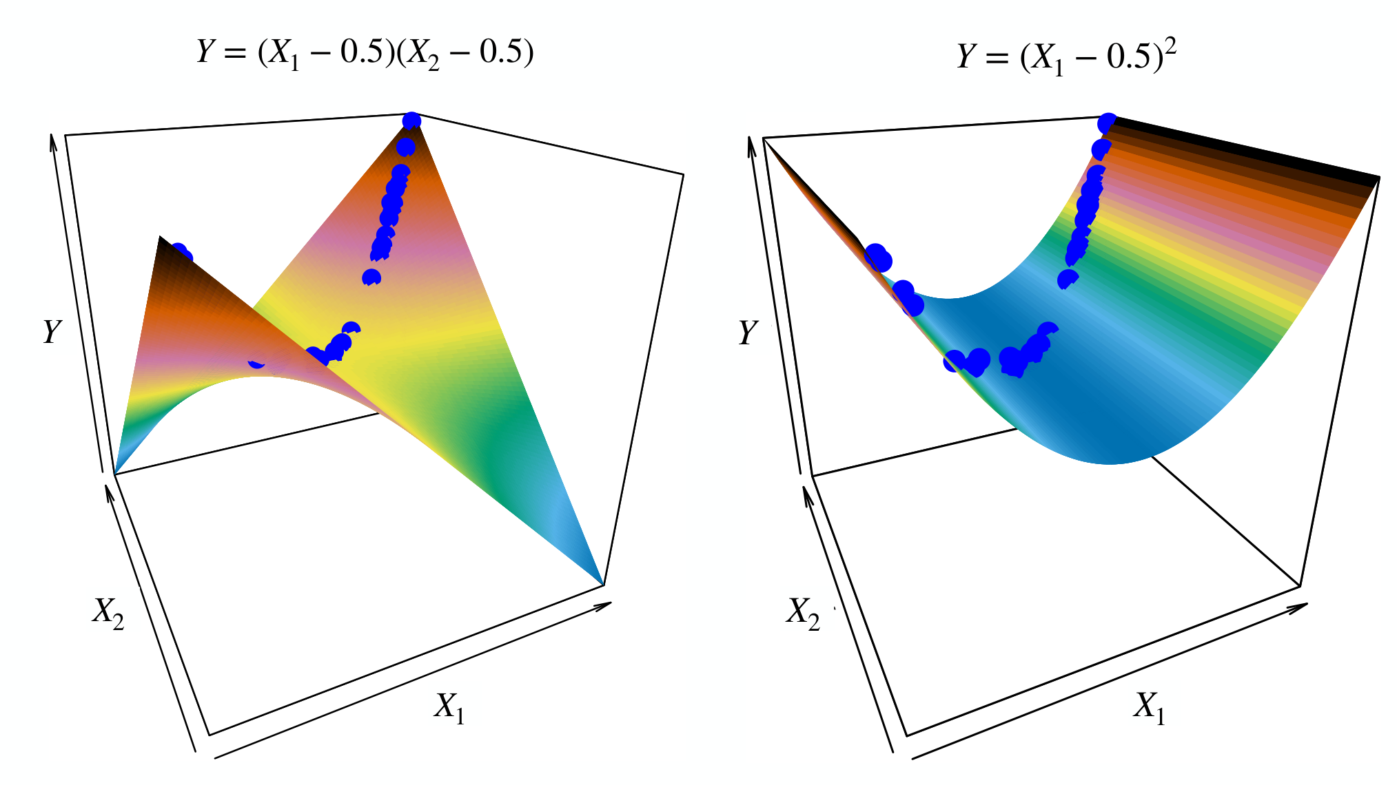
Figure 1: An example of an interaction that can be well approximated by the squared terms of either main effects when the two main effects are highly correlated. While the two surfaces are quite different, the perfect collinearity between X1X_{1} and X2X_{2} mean that all the observations (blue dots) fall along a line in which the interaction surface (on the left panel) can be perfectly explained by the squared-term surface involving only X1X_{1} (on the right panel).

Figure 1 shows an example where the interaction between two main effects can be very well approximated by either squared effect when these two constituent main effects are highly correlated. Given the widespread occurrence of feature correlation, especially in high-dimensional settings, our focus on 𝒈j={Xj,Xj2}\bm{g}_{j}=\{X_{j},X_{j}^{2}\} in (2) is particularly relevant in practice. In a more general setting where specific interactions may be strongly correlated with linear combinations of the univariate functions of main effects f1∗​(X1),…,fp∗​(Xp)f^{\ast}_{1}(X_{1}),\ldots,f^{\ast}_{p}(X_{p}), we could get equivalently predictive models without using that interaction.

Such logic is not restricted to continuous predictors. Consider a simple model Y=X1+X2+X1​X2Y=X_{1}+X_{2}+X_{1}X_{2}, where X1=𝟙AX_{1}=\mathbbm{1}_{A} and X2=𝟙BX_{2}=\mathbbm{1}_{B} are the indicator variables of events AA and BB, respectively. Suppose further that with high probability A⊆BA\subseteq B, so that X1​X2=𝟙A​𝟙B=𝟙A∩B≈𝟙AX_{1}X_{2}=\mathbbm{1}_{A}\mathbbm{1}_{B}=\mathbbm{1}_{A\cap B}\approx\mathbbm{1}_{A}; hence, the main effect X1=𝟙AX_{1}=\mathbbm{1}_{A} can be used in place of the interaction X1​X2X_{1}X_{2}, i.e., Y≈2​X1+X2Y\approx 2X_{1}+X_{2}. This main-effects-only explanation of YY is simpler to understand and yet explains YY nearly as well as the original model with the interaction term.

Leaning on main effects more heavily than interactions is advantageous for at least two reasons. First, main effects are easier to interpret than interactions. Thus when presented with two models that predict the response equivalently, we should favor the one that relies on fewer interactions. When putting forward a regression model with interactions, there is an implication that the included interactions were needed. Second, we will show in this paper that prioritizing main effects (or simple functions of main effects such as squared terms) can lead to great computational savings both in terms of time and memory. The key reason for these savings is that when pp is large, the total number of main effects is far smaller than the number of interactions.

We emphasize that the proposed reluctance to interactions is different from the well-known hierarchy assumption. While both simplify the search for interactions by focusing on certain main effects, our basic premise does not explicitly tie an interaction to its corresponding main effects. For example, an interaction X3​X4X_{3}X_{4} could be highly correlated with a linear combination of f1∗​(X1)f^{\ast}_{1}(X_{1}) and f2∗​(X2)f^{\ast}_{2}(X_{2}), which may lead us to exclude X3​X4X_{3}X_{4}. On the other hand, the interaction X3​X4X_{3}X_{4} will be kept if it cannot be explained by any additive functions of main effects. This logic is very different from the logic used in the hierarchy assumption.

3 The sprinter algorithm

In this section, we describe a new method, called sprinter, that is motivated by the idea of being reluctant to include interactions. As mentioned in Section 2, for the rest of this paper we focus on the special example where fj=θj​Xjf_{j}=\theta_{j}X_{j} or fj=θj​1​Xj+θj​2​Xj2f_{j}=\theta_{j1}X_{j}+\theta_{j2}X_{j}^{2}. The proposed method, for the case where fj​(Xj)=θj​Xjf_{j}(X_{j})=\theta_{j}X_{j} in (2), is given in Algorithm 1 and has three steps:

  • •

    In Step 1, we fit a lasso (or any other regression method) of the response as well as possible using only main effects. This step purposely gives preference to main effects, motivated by the idea of prioritizing main effects over interactions described in Section 2.

  • •

    In Step 2, we perform a single pass over all interactions to identify interaction signal that was not captured in Step 1. Because each of the 𝒪⁡(p2)\mathcal{O}(p^{2}) interactions is only computed and used once, this step requires far less time and memory than APL, which requires repeated passes over all interactions.

  • •

    In Step 3, we fit a lasso (or any other user-specified regression method) of the residual from Step 1 on all main effects and the interactions that were selected in Step 2. Depending on the screening criterion in Step 2, the total number of variables in Step 3 can be far smaller than 𝒪⁡(p2)\mathcal{O}(p^{2}), leading to large computational gains over APL.

The lasso in Step 1 and Step 3 could be substituted by other regression methods. We choose the lasso as an example for subsequent analysis. Throughout the paper, we let q=(p2+p)/2q=(p^{2}+p)/2 be the total number of pairwise interactions between pp main effects. On a sample level, we denote 𝐗=(𝐗1,…,𝐗p)∈ℝn×p\mathbf{X}=\left(\mathbf{X}_{1},\dots,\mathbf{X}_{p}\right)\in\mathbb{R}^{n\times p} as the design matrix with each column 𝐗j∈ℝn\mathbf{X}_{j}\in\mathbb{R}^{n} consisting of all observations of variable XjX_{j} (for j=1,…,pj=1,\dots,p). Similarly 𝐙∈ℝn×q\mathbf{Z}\in\mathbb{R}^{n\times q} is the sample matrix of Z=(X12,X1​X2,…,Xp−1​Xp,Xp2)Z=(X_{1}^{2},X_{1}X_{2},\dots,X_{p-1}X_{p},X_{p}^{2}), and 𝐲∈ℝn\mathbf{y}\in\mathbb{R}^{n} is the response vector. We let cor¯​(⋅,⋅)\overline{\mathrm{cor}}(\cdot,\cdot) and sd¯​(⋅)\overline{\mathrm{sd}}(\cdot) stand for the sample correlation and the sample standard deviation respectively.

Algorithm 1 sprinter (a lasso example)
Main effects 𝐗∈ℝn×p\mathbf{X}\in\mathbb{R}^{n\times p}, interactions 𝐙∈ℝn×q\mathbf{Z}\in\mathbb{R}^{n\times q}, response 𝐲∈ℝn\mathbf{y}\in\mathbb{R}^{n}, η>0\eta>0
Step 1:
Fit a lasso of the response 𝐲\mathbf{y} on 𝐗\mathbf{X}.
Compute the residual 𝐫=𝐲−𝐗​θ^\mathbf{r}=\mathbf{y}-\mathbf{X}\hat{\theta}.
Step 2:
For a tuning parameter η\eta, screen based on the residual:
ℐ^η={ℓ∈[q]:sd¯​(𝐫)​|cor¯​(𝐙ℓ,𝐫)|>η},\displaystyle\hat{\mathcal{I}}_{\eta}=\left\{\ell\in[q]:\overline{\mathrm{sd}}(\mathbf{r})|\overline{\mathrm{cor}}\left(\mathbf{Z}_{\ell},\mathbf{r}\right)|>\eta\right\}, (3)
Step 3:
Fit a lasso of the residual 𝐫\mathbf{r} on 𝐗\mathbf{X} and 𝐙ℐ^η\mathbf{Z}_{\hat{\mathcal{I}}_{\eta}}:
(ξ^,φ^)∈arg​minξ∈ℝp,φ∈ℝ|ℐ^η|⁡{12​n​‖𝐫−𝐗​ξ−𝐙ℐ^η​φ‖22+λ⁡(‖ξ‖1+‖φ‖1)}.\displaystyle(\hat{\xi},\hat{\varphi})\in\argmin_{\xi\in\mathbb{R}^{p},\varphi\in\mathbb{R}^{|\hat{\mathcal{I}}_{\eta}|}}\left\{\frac{1}{2n}\left\lVert\mathbf{r}-\mathbf{X}\xi-\mathbf{Z}_{\hat{\mathcal{I}}_{\eta}}\varphi\right\rVert_{2}^{2}+\lambda\left(\left\lVert\xi\right\rVert_{1}+\left\lVert\varphi\right\rVert_{1}\right)\right\}. (4)
return (θ^+ξ^,φ^)(\hat{\theta}+\hat{\xi},\hat{\varphi})
For a new observation 𝐱\mathbf{x}, the predicted response would be 𝐱T​(θ^+ξ^)+𝐳ℐ^ηT​φ^\mathbf{x}^{T}(\hat{\theta}+\hat{\xi})+\mathbf{z}_{\hat{\mathcal{I}}_{\eta}}^{T}\hat{\varphi}.

For the case where fj=θj​1​Xj+θj​2​Xj2f_{j}=\theta_{j1}X_{j}+\theta_{j2}X_{j}^{2}, we simply move the squared effects from 𝐙\mathbf{Z} to 𝐗\mathbf{X} in Algorithm 1. For more general choices of fjf_{j} in (2), 𝐗\mathbf{X} could be replaced by any design matrix of 𝒪⁡(p)\mathcal{O}(p) variables derived from main effects (in such a case, Step 2 would still only consider interactions between the original pp main effects). For choices of fjf_{j} other than (2), one can simply change the fitting procedures in Step 1 and Step 3. Step 2 can be considered as a sure independence screening (Fan & Lv 2008; Barut et al. 2016, SIS;) of all interactions using the residual from Step 1.

These first two steps are built around the idea of being reluctant to include interactions. Given a set of highly correlated variables, the lasso tends to select just one of them. Thus, if an interaction is highly correlated with one or more main effects, APL may very well select the interaction. By contrast, sprinter explicitly prioritizes the main effects (in Step 1). An interaction will only be selected (in Step 2) if it can capture something in the signal that the main effects cannot. Finally, Step 3 jointly models the residual using main effects and the selected interactions, and the final model output is the combination of model fits in Step 1 and Step 3.

In practice, each step in Algorithm 1 involves a tuning parameter. In particular, there is a tuning parameter value triplet (λ1,η,λ3)(\lambda_{1},\eta,\lambda_{3}), where λ1\lambda_{1} and λ3\lambda_{3} are tuning parameters for the lasso in Step 1 and Step 3, respectively, and η\eta is for the screening in Step 2. The optimal value of these tuning parameters is usually unknown. One approach would be to select the tuning parameter triplet using a three-dimensional cross-validation, which could be computationally prohibitive. As an alternative, we consider screening in Step 2 using

ℐ^mtop={ℓ∈[q]:|cor¯​(𝐙ℓ,𝐫)|​ is among the ​m​ largest}.\displaystyle\hat{\mathcal{I}}_{m}^{\mathrm{top}}=\left\{\ell\in[q]:|\overline{\mathrm{cor}}\left(\mathbf{Z}_{\ell},\mathbf{r}\right)|\text{ is among the }m\text{ largest}\right\}. (5)

This top-mm approach is standard in screening based variable selection methods (Fan & Lv 2008; Barut et al. 2016) and large-scale interaction modeling approaches (Fan et al. 2016; Niu et al. 2018). Popular choices of values of mm include nn and ⌈n/log⁡(n)⌉\lceil n/\log(n)\rceil. In Section 5, we find that using m=⌈n/log⁡(n)⌉m=\lceil n/\log(n)\rceil consistently yields good performance, and cross-validating the value of mm has a rather small effect. The scaling of sd¯​(𝐫)\overline{\mathrm{sd}}(\mathbf{r}) is needed to facilitate the theoretical analysis of the scaling of η\eta (see, e.g., Theorem 3 and Theorem 4). Clearly, when the top-mm approach is used, the scaling of sd¯​(𝐫)\overline{\mathrm{sd}}(\mathbf{r}) is unnecessary.

With a fixed value of mm (and equivalently, η\eta), we only need a two-dimensional cross-validation of the lasso tuning parameter pair (λ1,λ3)(\lambda_{1},\lambda_{3}), which is computationally viable due to the efficient path algorithms (Friedman et al. 2010) for solving lasso problems in Step 1 and Step 3.

3.1 A computationally efficient variant

As we will see in Section 4, Step 1 only needs to yield a good residual to guarantee the performance of Algorithm 1. Therefore, we also consider the following computationally efficient variant of sprinter:

sprinter(1cv): in Algorithm 1, we first select the tuning parameter in Step 1 before proceeding to subsequent steps.

In Section 5, we find that in most settings, sprinter(1cv) is doing only slightly worse than sprinter with two-dimensional cross-validation of (λ1,λ3)(\lambda_{1},\lambda_{3}), with the benefit of faster computation. However, there are situations in which sprinter(1cv) would substantially fall short. For example, when there is no main effects signal, sprinter(1cv)’s Step 1 tends to under-penalize whereas sprinter, which simultaneously cross-validates (λ1,λ3)(\lambda_{1},\lambda_{3}), tends to pick a very large value of λ1\lambda_{1} and thus avoids this problem.

3.2 Computation

With a value of m≤nm\leq n, the required computation in both Step 1 and Step 3 are no worse than fitting a lasso with p+np+n features. However, the major computational burden lies in Step 2, where 𝒪⁡(p2)\mathcal{O}(p^{2}) sample correlations are computed. It is thus essential for this step to be implemented as efficiently as possible, both in terms of computational time and storage.

We compute the sample correlation between each interaction and the residual from Step 1 on the fly. In the meantime, a min-heap is used to keep the index pairs of the interactions that attain the mm largest sample correlations. This ensures that we do not have to store 𝒪⁡(p2)\mathcal{O}(p^{2}) elements. The time complexity of Step 2 is thus 𝒪⁡(p2​(n+log⁡m))\mathcal{O}(p^{2}(n+\log m)), where 𝒪⁡(p2​log⁡m)\mathcal{O}(p^{2}\log m) is for maintaining the mm largest elements in a data stream of size 𝒪⁡(p2)\mathcal{O}(p^{2}) by using a min-heap of size mm (Cormen et al. 2009). Note that the whole algorithm only requires 𝒪⁡(n⁡(p+m))\mathcal{O}(n(p+m)) storage. Various other data structures could be used to achieve similar computational and storage complexity. Step 2 could also be computed approximately using an equivalence with the correlation screening and closest-pair problems (Shamos & Hoey 1975; Agarwal et al. 1991), which could be solved approximately using locality sensitive hashing (Rajaraman & Ullman 2011; Thanei et al. 2018) with a much improved computational complexity that is subquadratic in pp.

3.3 Related methods

Our method is not alone in dropping the hierarchy assumption (Thanei et al. 2018; Fan et al. 2016; Niu et al. 2018; Reese et al. 2018; Wang et al. 2021; Zhou et al. 2019, see, e.g.,). Interaction pursuit (IP) operates in two stages, first seeking a subset of the original pp variables that are involved in the nonzero interactions and then restricting attention to interactions between these selected variables (Fan et al. 2016). This method is efficient and can be quite effective. Like multi-stage hierarchy methods and unlike our method, IP’s success hinges on successful screening in the first step. Screening is easiest when the interactions are concentrated among a small set of original variables. The most challenging situation for this method is when there is no such concentration of interactions over a small set of original variables. Other screening-based methods exist. Niu et al. 2018 select interactions based on the partial correlation between the response and each interaction, with the corresponding two main effects adjusted. Reese et al. 2018 screens interactions based on the three-way joint cumulant between the response and two main effects that make up an interaction. While these two methods account for the exact two main effects when selecting an interaction, our proposal is more general in that it will only select an interaction that cannot be explained by any linear combinations of all main effects. Furthermore, our method is accompanied by finite sample theoretical guarantees, while such guarantees are not currently available for the methodology in Niu et al. 2018 and Reese et al. 2018. Thanei et al. 2018 consider a randomized algorithm that solves each step of APL approximately by solving a closest-pair problem. By doing so, they show that the computational complexity of their method is sub-quadratic in pp. Our method, while still having the same worst-case time complexity as that of APL, appears to be as fast as Thanei et al. 2018 in practice, and we find in our experiments it gives better predictive performance.

4 Theoretical analysis

Model (1) expresses the signal in terms of a main effects signal term, XT​β∗X^{T}\beta^{\ast}, and an interactions signal term, ZT​γ∗Z^{T}\gamma^{\ast}. If XX and ZZ were uncorrelated, this would be a unique decomposition. However, as demonstrated in Section 2, there can be “overlap” between these two signal terms. Let XT​ϑ∗X^{T}\vartheta^{\ast} be the part of ZT​γ∗Z^{T}\gamma^{\ast} that can be explained by a linear combination of XX, i.e.,

ϑ∗:=arg​minϑ∈ℝp⁡Var​(ZT​γ∗−XT​ϑ)=Cov​(X)−1​Cov​(X,Z)​γ∗=Σ−1​Φ​γ∗,\displaystyle\vartheta^{\ast}:=\argmin_{\vartheta\in\mathbb{R}^{p}}\mathrm{Var}\left(Z^{T}\gamma^{\ast}-X^{T}\vartheta\right)=\mathrm{Cov}\left(X\right)^{-1}\mathrm{Cov}\left(X,Z\right)\gamma^{\ast}=\Sigma^{-1}\Phi\gamma^{\ast}, (6)

where we denote Σ=Cov⁡(X)∈ℝp×p\Sigma=\mathrm{Cov}(X)\in\mathbb{R}^{p\times p} and Φ=Cov⁡(X,Z)∈ℝp×q\Phi=\mathrm{Cov}(X,Z)\in\mathbb{R}^{p\times q}. We can then write (1) as

Y=XT​θ∗+WT​γ∗+ε,\displaystyle Y=X^{T}\theta^{\ast}+W^{T}\gamma^{\ast}+\varepsilon, (7)

where θ∗=β∗+ϑ∗\theta^{\ast}=\beta^{\ast}+\vartheta^{\ast}, and

W:=Z−ΦT​Σ−1​X\displaystyle W:=Z-\Phi^{T}\Sigma^{-1}X

is the “pure” interaction effects that cannot be captured by linear combinations of XX, with Cov⁡(X,W)=0\mathrm{Cov}(X,W)=0. We denote the covariance of the pure interactions as

Ω:=Cov⁡(W)=Cov⁡(Z,W)=Cov⁡(Z)−Cov⁡(Z,X)​Σ−1​Φ=Ψ−ΦT​Σ−1​Φ,\displaystyle\Omega:=\mathrm{Cov}(W)=\mathrm{Cov}\left(Z,W\right)=\mathrm{Cov}\left(Z\right)-\mathrm{Cov}\left(Z,X\right)\Sigma^{-1}\Phi=\Psi-\Phi^{T}\Sigma^{-1}\Phi, (8)

where Ψ=Cov⁡(Z)∈ℝq×q\Psi=\mathrm{Cov}(Z)\in\mathbb{R}^{q\times q}. We note that XT​θ∗X^{T}\theta^{\ast} is aligned with the best population linear approximation to YY in Buja et al. 2019. By fitting YY using only linear combinations of XX, we fit a misspecified model because the pure interaction WW is ignored. We will see in the following analysis that the zero covariance structure between XX and WW is helpful in reducing the effects of this model misspecification. Actually, the benefit from the “orthogonality” between main effects and interactions is also observed in Hao & Zhang 2014, where XX is assumed to follow a zero-mean symmetric distribution. In such a case, we have that Φ=Cov⁡(X,Z)=0\Phi=\mathrm{Cov}(X,Z)=0, which implies that ϑ∗=0\vartheta^{\ast}=0 and W=ZW=Z. Our method does not require the symmetry of the distribution of main effects and thus allows for more general covariance structure between main effects XX and interactions ZZ.

We also note that XX in (7) can be generalized to be a random vector containing main effects and simple functions of main effects, e.g., the squared effects, or general univariate nonlinear functions of main effects fj​(Xj)f_{j}(X_{j})’s (as in Section 2).

To study sprinter’s performance, we will need to make assumptions about the tail behavior of the features. If main effects are sub-Gaussian, then their interactions are known to be sub-exponential. However, the analysis of interaction modeling usually involves the product of more than two main effects (e.g., the product of a main effect and an interaction), which has heavier tails than sub-exponential random variables. The following definition (Kuchibhotla & Chakrabortty 2022, Definition 2.2 and 2.4) will therefore be useful.

Definition 1 (sub-Weibull​(ν)\text{sub}\text{-Weibull}(\nu) random variable/vector).

A random variable UU is a sub-Weibull random variable of order ν>0\nu>0, i.e., sub-Weibull​(ν)\text{sub}\text{-Weibull}(\nu), if

‖U‖ψν=inf{ζ>0:E⁡[exp⁡(|U|νζν)]≤2}<∞,\displaystyle\|U\|_{\psi_{\nu}}=\inf\left\{\zeta>0:\mathrm{E}\left[\exp\left(\frac{|U|^{\nu}}{\zeta^{\nu}}\right)\right]\leq 2\right\}<\infty, (9)

where ‖U‖ψν\|U\|_{\psi_{\nu}} is the Orlicz norm of UU. A random vector V∈ℝpV\in\mathbb{R}^{p} is a sub-Weibull​(ν)\text{sub}\text{-Weibull}(\nu) random vector if cT​Vc^{T}V is a sub-Weibull​(ν)\text{sub}\text{-Weibull}(\nu) random variable for any constant vector c∈ℝpc\in\mathbb{R}^{p}. Furthermore, we define ‖V‖ψν=sup‖c‖2=1‖cT​V‖ψν\|V\|_{\psi_{\nu}}=\sup_{\|c\|_{2}=1}\|c^{T}V\|_{\psi_{\nu}}.

The notion of sub-Weibull​(ν)\text{sub}\text{-Weibull}(\nu) generalizes the definition of sub-Gaussian, which is sub-Weibull​(2)\text{sub}\text{-Weibull}(2), and sub-exponential, which is sub-Weibull​(1)\text{sub}\text{-Weibull}(1). In this paper, we are primarily interested in the cases where ν<1\nu<1. In particular, the product of three and four sub-Gaussian main effects, which as shown in Appendix A, are sub-Weibull​(2/3)\text{sub}\text{-Weibull}(2/3) and sub-Weibull​(1/2)\text{sub}\text{-Weibull}(1/2) respectively. In Appendix A, we also give a set of concentration inequalities for these heavy tailed random variables.

In the theoretical analysis of our method, we make the following assumptions:

  1. A1

    We have nn independent samples from (1), where X=(X1,…,Xp)X=(X_{1},\dots,X_{p}) follows a zero-mean sub-Gaussian distribution with covariance matrix Σ\Sigma and sub-Gaussian norm ‖X‖ψ2\|X\|_{\psi_{2}}, and ε\varepsilon is zero-mean sub-Gaussian noise independent of XX with Var⁡(ε)=σ2\mathrm{Var}(\varepsilon)=\sigma^{2}.

  2. A2

    We assume that κ​log⁡p≤n\kappa\log p\leq\sqrt{n} with some constant κ>1\kappa>1.

Assumption A1 is a very general distributional assumption on the random design; unlike other methods in high-dimensional interaction modeling, we do not require the distribution of XX to be symmetric. Assumption A2 is a standard assumption for pairwise interaction screening consistency (Hao & Zhang 2014, see, e.g., Assumption (C4) of). This is more stringent than the standard sample size requirement in main effects screening (Fan & Lv 2008, see, e.g., ), which requires log⁡p=𝒪⁡(n)\log p=\mathcal{O}(n). This is because interactions concentrate around their population means more slowly due to their heavier tails.

Ultimately we want to characterize the prediction performance and computational complexity of sprinter. In particular, the prediction error is characterized by

12​n​‖𝐗​θ∗+𝐖​γ∗−𝐗​θ^−𝐗​ξ^−𝐙ℐ^η​φ^‖22,\displaystyle\frac{1}{2n}\left\lVert\mathbf{X}\theta^{\ast}+\mathbf{W}\gamma^{\ast}-\mathbf{X}\hat{\theta}-\mathbf{X}\hat{\xi}-\mathbf{Z}_{\hat{\mathcal{I}}_{\eta}}\hat{\varphi}\right\rVert_{2}^{2},

where θ^\hat{\theta} is the Step 1 coefficient estimate of θ∗\theta^{\ast} in (7), (ξ^,φ^)(\hat{\xi},\hat{\varphi}) is the coefficient estimate from (4) given in Step 3 of Algorithm 1, and ℐ^η\hat{\mathcal{I}}_{\eta} is the output of Step 2 in (3) with tuning parameter η\eta.

Clearly, by taking η=0\eta=0, we have ℐ^η=[q]\hat{\mathcal{I}}_{\eta}=[q]. In this case, there is no computational gain over APL because all interactions will be considered in Step 3. On the other extreme, if η=∞\eta=\infty, then ℐ^η=∅\hat{\mathcal{I}}_{\eta}=\emptyset and the whole procedure ignores all of the pure interaction signal WT​γ∗W^{T}\gamma^{\ast}. Therefore, the success of sprinter hinges on capturing a small set ℐ^η\hat{\mathcal{I}}_{\eta} that still captures enough of the pure interaction signal WT​γ∗W^{T}\gamma^{\ast}.

We define the target set of interactions to recover as

ℐ(α)∈arg​max𝒜⊆[q]{minℓ∈𝒜|Ψℓ​ℓ−1/2Cov(Zℓ,WTγ∗)|s.t.∥(W𝒜CTγ𝒜C∗)2∥ψ1/2≤α}.\displaystyle\mathcal{I}(\alpha)\in\argmax_{\mathcal{A}\subseteq[q]}\left\{\min_{\ell\in\mathcal{A}}\left|\Psi_{\ell\ell}^{-1/2}\mathrm{Cov}\left(Z_{\ell},W^{T}\gamma^{\ast}\right)\right|\mathrm{\quad s.t.\quad}\|(W_{\mathcal{A}^{C}}^{T}\gamma_{\mathcal{A}^{C}}^{\ast})^{2}\|_{\psi_{1/2}}\leq\alpha\right\}. (10)

We first explain the constraint in (10). Recall that WT​γ∗W^{T}\gamma^{\ast} is the part of the interaction signal that cannot be explained by linear combinations of main effects. In Appendix A we show that (WT​γ∗)2(W^{T}\gamma^{\ast})^{2} is a sub-Weibull​(1/2)\text{sub}\text{-Weibull}(1/2) random variable. For any value α≥0\alpha\geq 0, we call a set 𝒜⊆[q]\mathcal{A}\subseteq[q] of interactions α\alpha-important if ‖(W𝒜CT​γ𝒜C∗)2‖ψ1/2≤α\|(W^{T}_{\mathcal{A}^{C}}\gamma^{\ast}_{\mathcal{A}^{C}})^{2}\|_{\psi_{1/2}}\leq\alpha.

Remark 2.

Lemma 8 (in Appendix A) shows that E⁡[(W𝒜CT​γ𝒜C∗)2]≤4​‖(W𝒜CT​γ𝒜C∗)2‖ψ1/2≤4​α\mathrm{E}[(W^{T}_{\mathcal{A}^{C}}\gamma^{\ast}_{\mathcal{A}^{C}})^{2}]\leq 4\|(W^{T}_{\mathcal{A}^{C}}\gamma^{\ast}_{\mathcal{A}^{C}})^{2}\|_{\psi_{1/2}}\leq 4\alpha. Therefore, an α\alpha-important set of interactions captures all but 4​α4\alpha of the pure interaction signal.

Here, α\alpha is a theoretical tuning parameter controlling the size of the target (population-level) screening set ℐ⁡(α)\mathcal{I}(\alpha) in Step 2, thereby determining the trade-off between computation and prediction error. In typical interaction modeling, the goal would be to recover supp⁡(γ∗)\operatorname{supp}(\gamma^{\ast}), which is a 00-important set; however, by taking larger α\alpha, we can reduce the size of the target interaction screening set, improving computation with controlled cost to prediction error. In our reluctant interaction selection framework, we do not care about recovering a set of interactions ℬ⊆supp⁡(γ∗)\mathcal{B}\subseteq\operatorname{supp}(\gamma^{\ast}) if ‖(WℬT​γℬ∗)2‖ψ1/2\|(W_{\mathcal{B}}^{T}\gamma^{\ast}_{\mathcal{B}})^{2}\|_{\psi_{1/2}} (and thus E⁡[(WℬT​γℬ∗)2]\mathrm{E}[(W_{\mathcal{B}}^{T}\gamma^{\ast}_{\mathcal{B}})^{2}]) is small. For example, if ZℓZ_{\ell} can be perfectly explained by a linear combination of main effects, then we do not wish to select interaction ℓ\ell even if γℓ∗≠0\gamma_{\ell}^{\ast}\neq 0. A strength of our theoretical results is that they are in terms of general α\alpha, thus making explicit the trade-off between computational efficiency and prediction accuracy.

From (10) we know that ℐ⁡(α)\mathcal{I}(\alpha) is an α\alpha-important set. Yet for any α≥0\alpha\geq 0, the α\alpha-important set is not necessarily unique. If Step 1 does a good job of capturing all the signal from the main effects, i.e., 𝐗​θ∗≈𝐗​θ^\mathbf{X}\theta^{\ast}\approx\mathbf{X}\hat{\theta}, where 𝐗​θ^\mathbf{X}\hat{\theta} is the fitted response from Step 1, then 𝐫=𝐲−𝐗​θ^\mathbf{r}=\mathbf{y}-\mathbf{X}\hat{\theta} should essentially be the pure interaction signal 𝐖​γ∗\mathbf{W}\gamma^{\ast} (with noise). Step 2 obtains ℐ^η\hat{\mathcal{I}}_{\eta} by including all the interactions whose (scaled) sample correlation with the residual is large enough, i.e., ωℓ=sd¯​(𝐫)​|cor¯​(𝐙ℓ,𝐫)|≥η\omega_{\ell}=\overline{\mathrm{sd}}(\mathbf{r})|\overline{\mathrm{cor}}\left(\mathbf{Z}_{\ell},\mathbf{r}\right)|\geq\eta for some η≥0\eta\geq 0, where ωℓ\omega_{\ell} is a noisy proxy of the population signal strength

ωℓ∗=Ψℓ​ℓ−1/2Cov(Zℓ,WTγ∗).\omega^{\ast}_{\ell}=\Psi_{\ell\ell}^{-1/2}\mathrm{Cov}(Z_{\ell},W^{T}\gamma^{\ast}).

For any α\alpha-important set 𝒜\mathcal{A} to be detectable, we require that the minimum signal strength minℓ∈𝒜⁡|ωℓ∗|\min_{\ell\in\mathcal{A}}|\omega_{\ell}^{\ast}| in 𝒜\mathcal{A} is large enough to be differentiated from the noise. The target set of interactions ℐ⁡(α)\mathcal{I}(\alpha) in (10) is thus defined as the α\alpha-important set that is most easily detected since it has the largest minimum signal strength, which we define as

η⁡(α):=12​minℓ∈ℐ⁡(α)​|ωℓ∗|.\displaystyle\eta(\alpha):=\frac{1}{2}\min_{\ell\in\mathcal{I}(\alpha)}|\omega_{\ell}^{\ast}|. (11)

The following theorem shows the main theoretical properties of sprinter: it attains good prediction accuracy while being computationally efficient when the minimum signal strength is greater than a certain noise level. We provide a roadmap to its proof in Section 4.1, deferring the full proof of this and all other results to the appendix.

Theorem 3.

Define

η∗=\displaystyle\eta^{\ast}= K[(∥diag(Ψ)−1/2Z∥ψ1∥WTγ∗∥ψ1+maxℓ|ωℓ∗|)(log⁡p)3/4n1/2\displaystyle K\left[\left(\|\operatorname{diag}(\Psi)^{-1/2}Z\|_{\psi_{1}}\|W^{T}\gamma^{\ast}\|_{\psi_{1}}+\max_{\ell}|\omega_{\ell}^{\ast}|\right)\frac{(\log p)^{3/4}}{n^{1/2}}\right.
+(σ+∥WTγ∗∥ψ1)1/2∥X∥ψ21/2(log⁡p)1/4n1/4+σ(log⁡p)1/2n1/2],\displaystyle\left.+\left(\sigma+\|W^{T}\gamma^{\ast}\|_{\psi_{1}}\right)^{1/2}\|X\|_{\psi_{2}}^{1/2}\frac{(\log p)^{1/4}}{n^{1/4}}+\sigma\frac{(\log p)^{1/2}}{n^{1/2}}\right], (12)

to be the noise level, where K>0K>0 is a constant. Under Assumption A1 and A2, for any α≥0\alpha\geq 0, under the signal strength condition that η⁡(α)≥η∗\eta(\alpha)\geq\eta^{\ast}, and taking

λ0=C⁡(σ+‖WT​γ∗‖ψ1)​‖X‖ψ2​log⁡pn,λ=C1​σ​max⁡(‖X‖ψ2,‖Z‖ψ1)​log⁡pn\displaystyle\lambda_{0}=C\left(\sigma+\|W^{T}\gamma^{\ast}\|_{\psi_{1}}\right)\|X\|_{\psi_{2}}\sqrt{\frac{\log p}{n}},\qquad\lambda=C_{1}\sigma\max\left(\|X\|_{\psi_{2}},\|Z\|_{\psi_{1}}\right)\sqrt{\frac{\log p}{n}} (13)

as the tuning parameter value in Step 1 and Step 3 respectively, then for any η∈[η∗,η⁡(α)]\eta\in[\eta^{\ast},\eta(\alpha)], sprinter achieves:

  1. 1.

    (Screening property, implying computational efficiency)

    ℐ(α)⊆ℐ^ηand|ℐ^η|≤4η−2λmax(diag(Ψ)−1/2Ωdiag(Ψ)−1/2)Var(WTγ∗)\displaystyle\mathcal{I}(\alpha)\subseteq\hat{\mathcal{I}}_{\eta}\quad\text{and}\quad|\hat{\mathcal{I}}_{\eta}|\leq 4{\eta}^{-2}\lambda_{\max}\left(\operatorname{diag}(\Psi)^{-1/2}\Omega\operatorname{diag}(\Psi)^{-1/2}\right)\mathrm{Var}(W^{T}\gamma^{\ast}) (14)
  2. 2.

    (Prediction error rate)

    12​n​‖𝐗​θ∗−𝐗​θ^+𝐖​γ∗−𝐗​ξ^−𝐙ℐ^η​φ^‖22\displaystyle\frac{1}{2n}\left\lVert\mathbf{X}\theta^{\ast}-\mathbf{X}\hat{\theta}+\mathbf{W}\gamma^{\ast}-\mathbf{X}\hat{\xi}-\mathbf{Z}_{\hat{\mathcal{I}}_{\eta}}\hat{\varphi}\right\rVert_{2}^{2}
    ≤\displaystyle\leq C2​(‖WT​γ∗‖ψ1​‖X‖ψ2​log⁡pn+λ)​‖θ∗‖1\displaystyle C_{2}(\|W^{T}\gamma^{\ast}\|_{\psi_{1}}\|X\|_{\psi_{2}}\sqrt{\frac{\log p}{n}}+\lambda)\|\theta^{\ast}\|_{1}
    +infα¯≥α{C3α¯+4λ(∥Σ−1Φℐ⁡(α¯)γℐ⁡(α¯)∗∥1+∥γℐ⁡(α¯)∗∥1)}\displaystyle+\inf_{\bar{\alpha}\geq\alpha}\left\{C_{3}\bar{\alpha}+4\lambda\left(\|\Sigma^{-1}\Phi_{\mathcal{I}(\bar{\alpha})}\gamma^{\ast}_{\mathcal{I}(\bar{\alpha})}\|_{1}+\|\gamma^{\ast}_{\mathcal{I}(\bar{\alpha})}\|_{1}\right)\right\} (15)

with probability greater than 1−2​exp⁡(−n3/5)−2​p−1−16​p−2​(κ1/3−1)1-2\exp\left(-n^{3/5}\right)-2p^{-1}-16p^{-2(\kappa^{1/3}-1)}, where C1,C2C_{1},C_{2}, and C3C_{3} are positive constants.

The value of η∗\eta^{\ast} in (12) is the noise level in Step 2, which is the sum of three terms: the first term depends on the strength of the pure interaction signal. The second term stems from the prediction error bound from Step 1, which fits a misspecified model since it ignores the pure interaction signal WT​γ∗W^{T}\gamma^{\ast} in (7). The last term depends on the error standard deviation σ\sigma. Actually from Theorem 7 we see that the second term is a slow rate prediction error bound for Step 1. The results in Theorem 3 can thus be generalized by replacing the second term with a faster rate under stronger assumptions if lasso is still used in Step 1, or any other prediction error bound available to a generic method used in Step 1. In such a generalization, only the second term in η∗\eta^{\ast} and the probability with which (14) and (15) hold will be changed.

The result in (14) characterizes the size of retained interactions used in Step 3. In particular, it implies that if Var⁡(WT​γ∗)=0\mathrm{Var}(W^{T}\gamma^{\ast})=0, i.e., if all interaction signal can be explained by main effects, then ℐ^η=∅\hat{\mathcal{I}}_{\eta}=\emptyset, and Step 3 is not needed at all. Finally, the results in Theorem (3) hold with probability tending to 11 as p→∞p\rightarrow\infty and n→∞n\rightarrow\infty.

Computationally, recall that Step 3 of sprinter is solving a lasso with O⁡(p+|ℐ^η|)O(p+|\hat{\mathcal{I}}_{\eta}|) variables. If |ℐ^η|=o⁡(p2)|\hat{\mathcal{I}}_{\eta}|=o(p^{2}), then Step 3 of sprinter is computationally more efficient than APL because it solves a problem with a smaller number of variables. By the orthogonality between XX and WW, we have Var⁡(Y)=Var⁡(XT​θ∗)+Var⁡(WT​γ∗)+σ2\mathrm{Var}(Y)=\mathrm{Var}(X^{T}\theta^{\ast})+\mathrm{Var}(W^{T}\gamma^{\ast})+\sigma^{2}. Under a standard assumption that Var⁡(Y)=𝒪⁡(1)\mathrm{Var}(Y)=\mathcal{O}(1) (Fan & Lv 2008, see, e.g.,), if the maximum singular value λmax(diag(Ψ)−1/2Ωdiag(Ψ)−1/2)=o(η∗2p2)\lambda_{\max}\left(\operatorname{diag}(\Psi)^{-1/2}\Omega\operatorname{diag}(\Psi)^{-1/2}\right)=o({\eta^{\ast}}^{2}p^{2}), then (17) implies that |ℐ^η|=o⁡(p2)|\hat{\mathcal{I}}_{\eta}|=o(p^{2}) and thus sprinter is computationally more efficient than APL.

In Section 4.2 we consider an example, where we explicitly write out the condition under which the condition η⁡(α)≥η∗\eta(\alpha)\geq\eta^{\ast} holds for different values of α\alpha.

4.1 A roadmap to the proof of Theorem 3

In this section, we give a series of theoretical results derived in order to prove Theorem 3. As discussed in the previous section, the success of Step 3 depends on Step 2 achieving a type of screening property, i.e., it retaining all the important interactions in ℐ⁡(α)\mathcal{I}(\alpha), and also that |ℐ^η||\hat{\mathcal{I}}_{\eta}| is not too large. The following theorem shows that if the signal strength condition that η⁡(α)≥η∗\eta(\alpha)\geq\eta^{\ast} holds, then Step 2 yields a small screening set that contains ℐ⁡(α)\mathcal{I}(\alpha).

Theorem 4 (Screening property in Step 2).

Consider the event

ℰR={n−1/2∥𝐗θ∗−𝐗θ^∥2≤R}\mathcal{E}_{R}=\left\{n^{-1/2}\|\mathbf{X}\theta^{\ast}-\mathbf{X}\hat{\theta}\|_{2}\leq R\right\}

for some prediction error rate RR of Step 1. Let

η¯∗=K[(∥diag(Ψ)−1/2Z∥ψ1∥WTγ∗∥ψ1+maxℓ|ωℓ∗|)(log⁡p)3/4n1/2+R+σ(log⁡p)1/2n1/2],\displaystyle\bar{\eta}^{\ast}=K\left[\left(\|\operatorname{diag}(\Psi)^{-1/2}Z\|_{\psi_{1}}\|W^{T}\gamma^{\ast}\|_{\psi_{1}}+\max_{\ell}|\omega_{\ell}^{\ast}|\right)\frac{(\log p)^{3/4}}{n^{1/2}}+R+\sigma\frac{(\log p)^{1/2}}{n^{1/2}}\right], (16)

where K>0K>0 is a constant. Under Assumption A1 and A2, for any α≥0\alpha\geq 0, if η⁡(α)≥η¯∗\eta(\alpha)\geq\bar{\eta}^{\ast}, then for any η∈[η¯∗,η⁡(α)]\eta\in[\bar{\eta}^{\ast},\eta(\alpha)],

ℐ(α)⊆ℐ^ηand|ℐ^η|≤4η−2λmax(diag(Ψ)−1/2Ωdiag(Ψ)−1/2)Var(WTγ∗)\displaystyle\mathcal{I}(\alpha)\subseteq\hat{\mathcal{I}}_{\eta}\quad\text{and}\quad|\hat{\mathcal{I}}_{\eta}|\leq 4{\eta}^{-2}\lambda_{\max}\left(\operatorname{diag}(\Psi)^{-1/2}\Omega\operatorname{diag}(\Psi)^{-1/2}\right)\mathrm{Var}(W^{T}\gamma^{\ast}) (17)

holds with probability greater than 1−8​p−2​(κ2/5−1)−2​p−1−Pr⁡(ℰRC)1-8p^{-2(\kappa^{2/5}-1)}-2p^{-1}-\mathrm{Pr}(\mathcal{E}_{R}^{C}).

As discussed in the previous section, for the set ℐ⁡(α)\mathcal{I}(\alpha) to be recovered, the condition that η⁡(α)≥η¯∗\eta(\alpha)\geq\bar{\eta}^{\ast} requires that the minimum signal strength η⁡(α)\eta(\alpha) should be stronger than η¯∗\bar{\eta}^{\ast}, which, intuitively can be considered as the noise level of Step 2. This is similar to a “β\beta-min” condition in the screening and variable selection consistency literature (Fan & Lv 2008; Wainwright 2009, see, e.g.,). The definition of η¯∗\bar{\eta}^{\ast} is more general than (12) in that it allows for a generic prediction error rate RR of Step 1. As a result, the probability with which (17) holds depends on Pr⁡(ℰRC)\mathrm{Pr}(\mathcal{E}_{R}^{C}). As discussed earlier, applying a different method in Step 1 or a different rate using lasso (under stronger conditions) will result in a different RR, which changes the bounds (and the corresponding probability) in Theorem 3.

As with other methods in interaction screening, we note that the result in Theorem 4 is less favorable (which is mostly reflected in a stricter sample size requirement A2) than that of sure independence screening (Fan & Lv 2008) in the main-effects-only case. This reveals an intrinsic challenge when dealing with interactions, namely that they have heavier tails than main effects. When we further assume that XX has a bounded distribution, Theorem 4 can be much improved. The rate is still less good than the main-effects-only case, as it depends on the misspecified lasso fit in the first step—an expected caveat in a two-stage method.

Remark 5 (The “top-mm” strategy).

Both η⁡(α)\eta(\alpha) and η¯∗\bar{\eta}^{\ast} depend on some population quantities, and thus are not available in practice. We thus adapt the same “top-mm” strategy as Fan & Lv 2008 and Fan et al. 2016 using ℐ^mtop\hat{\mathcal{I}}^{\mathrm{top}}_{m} of (5). Appendix F shows that Step 2 succeeds if we adapt the “top-mm” approach under certain conditions.

With Theorem 4 we have shown (14) in Theorem 3. To show (15), the following theorem first gives a deterministic bound on the prediction error of Step 3 if ℐ⁡(α)⊆ℐ^η\mathcal{I}(\alpha)\subseteq\hat{\mathcal{I}}_{\eta} holds.

Theorem 6 (Prediction error in Step 3).

Consider the event

ℰR={n−1/2∥𝐗θ∗−𝐗θ^∥2≤R}\mathcal{E}_{R}=\left\{n^{-1/2}\|\mathbf{X}\theta^{\ast}-\mathbf{X}\hat{\theta}\|_{2}\leq R\right\}

for some prediction error rate RR of Step 1. For any α≥0\alpha\geq 0, suppose ℐ⁡(α)⊆ℐ^η\mathcal{I}(\alpha)\subseteq\hat{\mathcal{I}}_{\eta}, and take

λ≥max⁡(1n​max1≤j≤p​|𝜺T​𝐗j|,1n​maxℓ∈ℐ^η​|𝜺T​𝐙ℓ|)\displaystyle\lambda\geq\max\left(\frac{1}{n}\max_{1\leq j\leq p}|\bm{\varepsilon}^{T}\mathbf{X}_{j}|,\frac{1}{n}\max_{\ell\in\hat{\mathcal{I}}_{\eta}}|\bm{\varepsilon}^{T}\mathbf{Z}_{\ell}|\right) (18)

as the tuning parameter value in Step 3. On the event ℰR\mathcal{E}_{R}, we have

12​n​‖𝐗​θ∗+𝐖​γ∗−𝐗⁡(θ^+ξ^)−𝐙ℐ^η​φ^‖22\displaystyle\frac{1}{2n}\left\lVert\mathbf{X}\theta^{\ast}+\mathbf{W}\gamma^{\ast}-\mathbf{X}(\hat{\theta}+\hat{\xi})-\mathbf{Z}_{\hat{\mathcal{I}}_{\eta}}\hat{\varphi}\right\rVert_{2}^{2}
≤\displaystyle\leq R2+1n​‖𝐖ℐ​(α)C​γℐ​(α)C∗‖22+2​λ​(‖Σ−1​Φℐ⁡(α)​γℐ⁡(α)∗‖1+‖γℐ⁡(α)∗‖1).\displaystyle R^{2}+\frac{1}{n}\left\lVert\mathbf{W}_{\mathcal{I}(\alpha)^{C}}\gamma^{\ast}_{\mathcal{I}(\alpha)^{C}}\right\rVert_{2}^{2}+2\lambda\left(\|\Sigma^{-1}\Phi_{\mathcal{I}(\alpha)}\gamma^{\ast}_{\mathcal{I}(\alpha)}\|_{1}+\|\gamma^{\ast}_{\mathcal{I}(\alpha)}\|_{1}\right). (19)

The result is deterministic in that it does not require any probabilistic argument. Based on Theorem 6, Theorem 3 then characterizes the scale of λ\lambda and the corresponding probability that (18) holds.

Finally, we derive a particular prediction error rate RR in Step 1 used in Theorem 4. Although the proposed framework does not depend on a specific regression method in Step 1 for fitting the main effects, we take the lasso as an example. Recall that in Step 1 we are fitting a misspecified model, i.e., we treat WT​γ∗+εW^{T}\gamma^{\ast}+\varepsilon in (7) as the noise term and solve the following problem:

θˇ∈arg​minθ⁡(12​n​‖𝐲−𝐗​θ‖22+λ​‖θ‖1).\check{\theta}\in\argmin_{\theta}\left(\frac{1}{2n}\left\lVert\mathbf{y}-\mathbf{X}\theta\right\rVert^{2}_{2}+\lambda\left\lVert\theta\right\rVert_{1}\right).

The following theorem gives a prediction error rate for the main effects only lasso that is carried out in Step 1.

Theorem 7 (Prediction error in Step 1).

Suppose that Assumption A1 and A2 hold. Take

λ0=C⁡(σ+‖WT​γ∗‖ψ1)​‖X‖ψ2​log⁡pn,\displaystyle\lambda_{0}=C\left(\sigma+\|W^{T}\gamma^{\ast}\|_{\psi_{1}}\right)\|X\|_{\psi_{2}}\sqrt{\frac{\log p}{n}},

where C>0C>0 is a constant, then for any λ≥λ0\lambda\geq\lambda_{0}, the following bound holds

1n​‖𝐗​θˇ−𝐗​θ∗‖22≤4​λ​‖θ∗‖1\displaystyle\frac{1}{n}\|\mathbf{X}\check{\theta}-\mathbf{X}\theta^{\ast}\|_{2}^{2}\leq 4\lambda\|\theta^{\ast}\|_{1}

with probability greater than 1−4​p−(κ1/3−1)1-4p^{-(\kappa^{1/3}-1)}.

We see, through λ\lambda’s dependence on ‖WT​γ∗‖ψ1\|W^{T}\gamma^{\ast}\|_{\psi_{1}}, that the presence of the pure interaction signal leads to rates that could be less good than if no interactions were present. This is the price paid for fitting a misspecified model in Step 1. Also this prediction bound holds under Assumption A2, which is a stricter sample size requirement due to dealing with the empirical process that involves interactions, which have heavier tails than main effects. This bound is aligned with the oracle inequality for the constrained lasso in the misspecified model (with a sub-Weibull(1) misspecification part). Under stronger conditions (e.g., compatibility conditions on θ∗\theta^{\ast}), a faster prediction error rate in Step 1 could be derived.

4.2 A Gaussian example

In this section we study the condition that η⁡(α)≥η∗\eta(\alpha)\geq\eta^{\ast} required both in Theorem 3 and Theorem 4 in the case where XX follows a Gaussian distribution. We defer the detailed computation to Appendix G, where we also consider an example where XX is not symmetric.

We let τ:[p]2→[q]\tau:[p]^{2}\rightarrow[q] map the interaction between XjX_{j} and XkX_{k} to its corresponding index in ZZ, i.e., Zτ⁡(j,k)=Xj​XkZ_{\tau(j,k)}=X_{j}X_{k}. Consider the simple case where X∼N⁡(𝟎,Σ)X\sim N(\mathbf{0},\Sigma), and there is only one true interaction, i.e., supp⁡(γ∗)={τ⁡(1,2)}\operatorname{supp}(\gamma^{\ast})=\{\tau(1,2)\}. Without loss of generality, we assume that Σj​j=1\Sigma_{jj}=1 for all j=1,…,pj=1,\dots,p, so that for any pair of variables XjX_{j} and XkX_{k}, their covariance σj​k\sigma_{jk} equals their correlation coefficient ρj​k\rho_{jk}. Recall from Section 2 that in the Gaussian case, Φ=𝟎\Phi=\mathbf{0}, W=ZW=Z and θ∗=β∗\theta^{\ast}=\beta^{\ast}. We discuss two cases, depending on the size of |γτ⁡(1,2)∗||\gamma_{\tau(1,2)}^{\ast}|:

  1. 1.

    (Strong interaction) Suppose the signal is strong in that

    |γτ⁡(1,2)∗|>r​(n,q)2,\displaystyle|\gamma^{\ast}_{\tau(1,2)}|>r(n,q)^{2},

    where

    r​(n,q)2=18​K2​‖β∗‖1​(log⁡pn)1/2+12​K​‖β∗‖11/2​σ1/2​(log⁡pn)1/4+12​K​σ​(log⁡pn)1/2,\displaystyle r(n,q)^{2}=18K^{2}\|\beta^{\ast}\|_{1}\left(\frac{\log p}{n}\right)^{1/2}+12K\|\beta^{\ast}\|_{1}^{1/2}\sigma^{1/2}\left(\frac{\log p}{n}\right)^{1/4}+12K\sigma\left(\frac{\log p}{n}\right)^{1/2},

    and K>0K>0 is the constant in (12). Appendix G shows that |γτ⁡(1,2)∗|>r​(n,q)2|\gamma^{\ast}_{\tau(1,2)}|>r(n,q)^{2} is a sufficient condition under which η⁡(α)≥η∗\eta(\alpha)\geq\eta^{\ast} holds for any α≥0\alpha\geq 0.

  2. 2.

    (Weak interaction) Suppose the signal strength is weak in that

    |γτ⁡(1,2)∗|≤r​(n,q)2.\displaystyle|\gamma^{\ast}_{\tau(1,2)}|\leq r(n,q)^{2}.

    Taking

    α=3​r​(n,q)4=𝒪⁡(σ​‖β∗‖1​(log⁡pn)1/2),\displaystyle\alpha=3r(n,q)^{4}=\mathcal{O}\left(\sigma\|\beta^{\ast}\|_{1}\left(\frac{\log p}{n}\right)^{1/2}\right), (20)

    we can show that ℐ⁡(α)=∅\mathcal{I}(\alpha)=\emptyset. As a result, (11) implies that η⁡(α)=∞\eta(\alpha)=\infty, which is trivially greater than η∗\eta^{\ast}.

Finally we note that the reason for condition η⁡(α)≥η∗\eta(\alpha)\geq\eta^{\ast} to be satisfied regardless of the size of the interaction signal strength is because of our focus on prediction error in Theorem 3 and Theorem 4 instead of the exact recovery of specific interactions.

5 Numerical studies

5.1 Simulation studies: binary features

We consider a simulation scenario with binary features in which some but not all interactions can be well approximated by main effects. We generate pp binary features as follows: for a (perfect) binary tree of depth dd, each leaf node is an independent Bernoulli(0.10.1) random variable; the value of each non-leaf node is the maximum of the node values in its sub-tree, i.e., each non-leaf node represents an event that is the union of all the events represented by its children nodes. The total number of nodes in the tree is p=2d+1−1p=2^{d+1}-1, and we consider these node values as main effects. This construction ensures that for any pair of main effects, they are either independent or else one is an ancestor of the other. The interaction between two binary features is simply the intersection of the two main effect events, so in this second case their interaction is simply the main effect corresponding to the descendant node. Figure 2 shows the binary tree (of depth 55), where each node represents a main effect, and the node color represents the success probability of the corresponding Bernoulli random variable.

Figure 2: An example of the perfect binary tree, representing main effects. Node color represents the success probability (rounded to 1 decimal place) of the corresponding Bernoulli random variable.

We can control the degree to which the interaction signal can be explained by main effects by choosing the proportion of nonzero elements of γ∗\gamma^{\ast} correspond to interactions between main effects that are ancestors/descendants of each other versus not. We consider three scenarios: (a) almost all interactions can be explained by main effects; (b) approximately half of the interactions can be explained by main effects; and (c) a very limited amount of interactions can be explained by main effects. These three scenario correspond to three cases where the main-effect-interaction-ratio,

MIR=‖𝐗​θ∗‖22‖𝐖​γ∗‖22,\displaystyle\mathrm{MIR}=\frac{\left\lVert\mathbf{X}\theta^{\ast}\right\rVert_{2}^{2}}{\left\lVert\mathbf{W}\gamma^{\ast}\right\rVert_{2}^{2}},

is large, medium, and small. We would expect sprinter to perform especially well when MIR\mathrm{MIR} is large. For each value of MIR, we generate the response 𝐲\mathbf{y} using (7) with the zero-mean additive noise ε\varepsilon generated according to the signal-to-noise ratio ‖𝐗​θ∗‖2+‖𝐖​γ∗‖2n​σ2∈{0.3,0.5,1,1.5,2,2.5,3}\frac{\left\lVert\mathbf{X}\theta^{\ast}\right\rVert^{2}+\left\lVert\mathbf{W}\gamma^{\ast}\right\rVert^{2}}{n\sigma^{2}}\in\left\{0.3,0.5,1,1.5,2,2.5,3\right\}. We generate n=100n=100 samples in each simulation setting, and in Figure 3 we report the prediction error (on another n=100n=100 testing samples) of various methods (averaged over 5050 repetitions). In particular, we compare the performance of the following methods:

  • •

    The all pairs lasso (APL) with tuning parameter selected by cross-validation. We use the R package glmnet to implement APL.

  • •

    sprinter, as in Algorithm 1, with lasso using main effects and squared effects in Step 1. In Step 2, we use the “top-mm approach” as in (5) with m=⌈n/log⁡(n)⌉m=\lceil n/\log(n)\rceil. We use a two-dimensional cross-validation to select (λ1,λ3)(\lambda_{1},\lambda_{3}), the tuning parameter pair for the lasso in Step 1 and Step 3, respectively. Both lasso fits are implemented using glmnet.

  • •

    The main effects lasso (MEL) with tuning parameter selected by cross-validation.

  • •

    SIS and Lasso: We use sure independence screening (Fan & Lv 2008) on all main effects and interactions, and fit the lasso on the selected candidate features.

  • •

    Interaction Pursuit (IP) by Fan et al. 2016.

Figure 3: Prediction mean-squared error of different methods (averaged over 50 repetitions, binary settings).

As MIR gets small, the performance of MEL worsens relative to other methods that model interactions. The performance of sprinter is favorable in comparison with other methods, especially when most of the signal can be well captured by main effects (as expected by the design of MIR\mathrm{MIR}). The third panel shows that APL achieves favorable performance compared with other methods when the signal is sufficiently strong and concentrated primarily in pure interactions. As we will see in subsequent simulation studies, the performance advantage of sprinter over APL is more pronounced when pp is much larger.

Furthermore, Figure 4 shows that the relationship between the number of selected interactions and the prediction error in the above three settings where the signal-to-noise ratio is 2. We observe that compared with IP, sprinter attains smaller prediction error using similar numbers of selected interactions. Compared with APL, sprinter selected a leaner set of interactions while achieving favorable prediction error (except in the last setting) .

Figure 4: Prediction mean-squared error v.s. the number of selected interactions. Each point represents one (out of 50) repetition.

5.2 Simulation studies: Gaussian features and hierarchy

Next we study the performance of sprinter under different interaction structures when the main effects follow a multivariate Gaussian distribution. We generate n=100n=100 samples from model (1), where XX is a pp-dimensional random vector following a multivariate zero-mean Gaussian distribution with Cov⁡(Xj,Xk)=0.5|j−k|\mathrm{Cov}(X_{j},X_{k})=0.5^{|j-k|} for 1≤j,k≤p1\leq j,k\leq p, and p=400p=400. Recall that our proposed idea of reluctance to interactions in Section 2 is different from the hierarchical principle for interactions, and the proposed method does not assume hierarchy; actually sprinter does not assume any structure among interactions. Denote 𝒯1\mathcal{T}_{1} as the indices of non-zero main effects, 𝒯2\mathcal{T}_{2} as the indices of non-zero squared terms and 𝒯3\mathcal{T}_{3} as indices of non-zero interaction terms, and consider the following structures for the interactions:

  1. 1.

    Mixed: 𝒯1={1,2,…,6},𝒯2={1,5,15},𝒯3={(1,5),(4,18),(10,11),(9,17),(1,13),(4,17)}\mathcal{T}_{1}=\left\{1,2,\dots,6\right\},\mathcal{T}_{2}=\left\{1,5,15\right\},\mathcal{T}_{3}=\left\{\left(1,5\right),\left(4,18\right),\left(10,11\right),\left(9,17\right),\left(1,13\right),\left(4,17\right)\right\}.

  2. 2.

    Hierarchical, i.e., βj​k≠0⟹βj≠0​ or ​βk≠0\beta_{jk}\neq 0\implies\beta_{j}\neq 0\text{ or }\beta_{k}\neq 0: 𝒯1={1,2,…,6}\mathcal{T}_{1}=\left\{1,2,\dots,6\right\} , 𝒯2={1,2,3}\mathcal{T}_{2}=\left\{1,2,3\right\} and 𝒯3={(1,3),(2,4),(3,4),(1,8),(2,8),(5,10)}\mathcal{T}_{3}=\left\{(1,3),(2,4),\left(3,4\right),(1,8),(2,8),(5,10)\right\}.

  3. 3.

    Anti-hierarchical, i.e., βj​k≠0⟹βj=0,βk=0\beta_{jk}\neq 0\implies\beta_{j}=0,\beta_{k}=0: 𝒯1={1,2,…,6}\mathcal{T}_{1}=\left\{1,2,\dots,6\right\}, 𝒯2={11,12,13}\mathcal{T}_{2}=\left\{11,12,13\right\} and 𝒯3={(11,13),(12,14),(13,14),(11,18),(12,18),(15,20)}\mathcal{T}_{3}=\left\{(11,13),(12,14),\left(13,14\right),(11,18),(12,18),(15,20)\right\}.

  4. 4.

    Interaction only: 𝒯1=𝒯2=∅\mathcal{T}_{1}=\mathcal{T}_{2}=\emptyset and 𝒯3={(1,3),(2,4),(3,4),(1,8),(2,8),(5,10)}\mathcal{T}_{3}=\left\{(1,3),(2,4),\left(3,4\right),(1,8),(2,8),(5,10)\right\}.

  5. 5.

    Main effects only: 𝒯1={1,2,…,6}\mathcal{T}_{1}=\left\{1,2,\dots,6\right\} , 𝒯2=∅\mathcal{T}_{2}=\emptyset and 𝒯3=∅\mathcal{T}_{3}=\emptyset.

  6. 6.

    Squared effects only: 𝒯1=∅\mathcal{T}_{1}=\emptyset , 𝒯2={1,2,…,6}\mathcal{T}_{2}=\left\{1,2,\dots,6\right\} and 𝒯3=∅\mathcal{T}_{3}=\emptyset.

Note that the hierarchy structure only exists in the hierarchical model and the main effects only model. The signal strength is then set as βj∗=2\beta^{\ast}_{j}=2 for j∈𝒯1j\in\mathcal{T}_{1}, γj∗=3\gamma^{\ast}_{j}=3 for j∈𝒯2j\in\mathcal{T}_{2} and j∈𝒯3j\in\mathcal{T}_{3}. Finally, the zero-mean additive noise ε\varepsilon in (1) is generated according to the signal-to-noise ratio ‖𝐗​β∗‖2+‖𝐙​γ∗‖2n​σ2∈{0.3,0.5,1,1.5,2,2.5,3}\sqrt{\frac{\left\lVert\mathbf{X}\beta^{\ast}\right\rVert^{2}+\left\lVert\mathbf{Z}\gamma^{\ast}\right\rVert^{2}}{n\sigma^{2}}}\in\left\{0.3,0.5,1,1.5,2,2.5,3\right\}.

In addition to the methods considered in the previous study, we also include the performance of the following two methods:

  • •

    sprinter(1cv), with everything the same as sprinter, except that cross-validation of λ1\lambda_{1} is performed before subsequent steps. See Section 3.1 for details.

  • •

    RAMP (Hao et al. 2018), which iteratively adds variables into a path of solutions under the marginality (hierarchy) principle. They also consider the two-stage lasso, but state that RAMP performs better than the two-stage lasso (Hao & Zhang 2014). The performance of RAMP is very unstable for binary features, and thus is not included in Section 5.1 or later in Section 5.4.

Figure 5: Prediction mean-squared error of different methods (averaged over 100 repetitions, Gaussian settings).

We measure the statistical performance of each method in prediction error, which is averaged over 100 repetitions and is reported in Figure 5. Observe that sprinter almost works uniformly better than other methods in all settings except in the model where main effects are dominating. This is because sprinter includes both main effects and the squared effects in Step 1, which involves pp irrelevant squared effects. Actually, although not shown here, sprinter works much better in this setting if it uses only main effects in Step 1.

We also note that the prediction performance advantage of sprinter over sprinter(1cv) is rather marginal, except for the interaction-only model. As discussed in Section 3.1, when there are only interactions in the model, sprinter(1cv) tends to under-penalize the main effects in the cross-validation of Step 1, and thus has much worse performance than sprinter.

5.3 Simulation studies: computation time

In this section, we show that sprinter is much more computationally efficient than APL, while having similar (if not better) statistical performance. To this end, we consider varying p∈{100,200,1000,2000}p\in\left\{100,200,1000,2000\right\} in the mixed model in Section 5.2 with signal-to-noise ratio equal to 33. The following plots show both the computation time (in seconds) and the prediction mean squared error (averaged over 100 repetitions).

Figure 6: Computation time and prediction mean-squared error (averaged over 100 repetitions) for different pp in the mixed model.

As expected, APL is computationally much more expensive than the proposed method. In particular, for p=2000p=2000, the proposed method is about 100 times faster than APL. In addition, while not shown, sprinter can solve a problem with 140000140000 main effects (about 10 billion interactions, which is infeasible for APL) with 5-fold cross-validation under 7 hours on a single CPU.

In addition to enjoying obvious computational benefits, the right panel of Figure 6 shows that the proposed method does not lose statistical performance in terms of prediction error. Actually, sprinter attains uniformly smaller prediction error than APL.

Furthermore, Figure 7 shows that compared with APL, sprinter achieves this favorable performance with a much smaller number of selected interactions (and more selected main effects) — a property that is expected by prioritizing main effects over interactions, and is beneficial for interpretation.

Figure 7: Number of non-zero main effects, interactions, and prediction mean-squared error for p=1000p=1000 in the mixed model. Each point represents one (out of 100) repetition.

5.4 Data example: Tripadvisor hotel reviews

We consider the dataset prepared in Wang et al. 2010, which contains reviews and the corresponding ratings (on the integer scale of {1,…,5}\{1,\ldots,5\}) of hotels on Tripadvisor.com. We further construct a dictionary, consisting of p=7817p=7817 distinct words following the approach in Yan & Bien 2020. Most of the words are adjectives, while we also include words that might alter the meaning of an adjective such as but, not, should, etc. In total, the dataset contains n=211321n=211321 reviews and is represented in the binary design matrix 𝐗∈ℝn×p\mathbf{X}\in\mathbb{R}^{n\times p}, where 𝐗i​j=1\mathbf{X}_{ij}=1 if the jj-th word in the dictionary appears in the ii-th review, and 𝐗i​j=0\mathbf{X}_{ij}=0 otherwise.

Our goal is to predict the hotel rating based on the words used in the review. While (1) is certainly an overly simplistic model for text data (especially in light of advances in natural language processing in recent years), the ability to easily interpret words makes this a helpful illustration of our method. Note that 𝐗i​j​𝐗i​k=1\mathbf{X}_{ij}\mathbf{X}_{ik}=1 indicates that both the jj-th word and the kk-th word appear in the ii-th review. The co-occurrence of two key words can provide useful information in the prediction task. For example, while a negative sounding word like “worst” might be associated with lower ratings, its co-occurrence with words like “not” (as in “not the worst”) would yield a very important interaction for prediction.

Due to memory constraints (that applies to all methods considered), we randomly select 10%10\% of the whole data as a training set, and the remaining 90%90\% as a testing set. We compare several methods: MEL, a two-stage hierarchical lasso (Hao et al. 2018, our implementation of a method proposed in), and sprinter. The problem size is too big for APL. In Table 1, we report the prediction root mean squared error on the testing set. In addition, we report the number of selected main effects and interactions. The performance of the other methods in previous sections is much worse, and thus are not included.

method prediction RMSE # main effects # interactions
MEL 1.153 689 0
Two Stage Hierarchical Lasso 1.125 500 992
sprinter 1.091 304 526
Table 1: Tripadvisor hotel reviews: prediction root mean squared error on the testing set, number of selected main effects and interactions

Comparing with sprinter, the prediction error of MEL suggests the importance of including interactions in the model, and the prediction error of the two-stage hierarchical lasso may suggest that the true underlying interaction structure is not hierarchical.

In the sprinter model, the top 55 main effects with largest positive coefficient estimates are excellent, fantastic, perfect, wonderful, and loved, while the top 55 main effects with largest negative coefficient estimates are worst, rude, poor, dirty, and awful. The sign and the magnitude of the coefficient estimates corresponding to these words are of course highly aligned with the words’ actual meanings.

The coefficient estimates for interactions are quite interesting. As expected, the interactions with the large positive coefficients include awful×\timesnot and rude×\timesbut. This makes sense since the words not and but often have the effect of negating or at least weakening the sentiment of the words around them. Interestingly, the coefficient corresponding to the interaction wonderful×\timessuperb and great ×\times fantastic have large negative estimate. We view this as reflecting the diminishing returns of superlative synonyms: a review containing both wonderful and superb does not make the rating twice as good as if the review only contains one of the words. The interaction serves to reduce the additive effects of the use of synonyms. This is especially sensible given that we are using presence-absence coding of words because it means that using wonderful and superb together is treated the same as if someone used wonderful twice.

6 Discussion

In this paper, we present sprinter (sparse reluctant interaction modeling), a general multi-step framework that is highly scalable to large interaction problems. Our proposal is motivated by a new guiding principle in interaction modeling, which favors main effects over interactions if all else is equal. We show, in both theoretical analysis and numerical studies, that sprinter achieves strong computational efficiency, without compromising favorable statistical properties.

Although not discussed in this paper, the sprinter framework can be easily generalized to higher order interaction modeling. The idea of screening interactions based on the residual from fitting a model of lower order terms can be used repeatedly to select higher order interactions. For example, after Step 3 of Algorithm 1, we could obtain a residual vector, which could then be used in screening three-way interactions. This approach can be used recursively in modeling higher order interactions, by prioritizing lower-order terms over higher-order terms if all else is equal.

The idea of enforcing reluctance to interactions could be further generalized to a broader context beyond interaction modeling. This is particularly useful when side information makes us prefer one group of variables over another. For example, one might be reluctant in using a group of expensive variables, and thus would try to capture the response as much as possible by first only using the group of cheap variables. This is an interesting future research direction.

One can also extend the proposed reluctant interaction modeling framework to using a general loss function ℓ\ell (e.g., as in generalized linear models), in which case the screening in Step 2 could be based on absolute correlation between each interaction and ∇ℓ\nabla\ell evaluated in Step 1.

Finally, an R (R Core Team 2018) package, named sprintr, is available online, implementing our method. The estimation is very fast with the core screening functions coded in Rcpp (Eddelbuettel & François 2011). The simulation studies in Section 5 use the simulator package (Bien 2016), and the code to reproduce all numerical studies is available at https://github.com/hugogogo/reproducible/tree/master/sprinter. The Tripadvisor data are available on request from the corresponding author. These data were derived from the following resources available in the public domain: http://times.cs.uiuc.edu/~wang296/Data/.

Acknowledgment

We thank Daniela Witten for helpful feedback. GY and JB were supported by NIH Grant R01GM123993. JB was also supported by NSF CAREER Award DMS-1653017. RT was supported by NSF CAREER Award DMS-1554123.

References

  • (1)
  • Agarwal et al. (1991) Agarwal, P. K., Edelsbrunner, H., Schwarzkopf, O. & Welzl, E. (1991), ‘Euclidean minimum spanning trees and bichromatic closest pairs’, Discrete & Computational Geometry 6(3), 407–422.
  • Barut et al. (2016) Barut, E., Fan, J. & Verhasselt, A. (2016), ‘Conditional sure independence screening’, Journal of the American Statistical Association 111(515), 1266–1277.
  • Bien (2016) Bien, J. (2016), ‘The Simulator: An Engine to Streamline Simulations’, ArXiv e-prints .
  • Bien et al. (2013) Bien, J., Taylor, J. & Tibshirani, R. (2013), ‘A lasso for hierarchical interactions’, Annals of statistics 41(3), 1111.
  • Buja et al. (2019) Buja, A., Brown, L., Berk, R., George, E., Pitkin, E., Traskin, M., Zhang, K., Zhao, L. et al. (2019), ‘Models as approximations i: Consequences illustrated with linear regression’, Statistical Science 34(4), 523–544.
  • Choi et al. (2010) Choi, N. H., Li, W. & Zhu, J. (2010), ‘Variable selection with the strong heredity constraint and its oracle property’, Journal of the American Statistical Association 105(489), 354–364.
  • Cormen et al. (2009) Cormen, T. H., Leiserson, C. E., Rivest, R. L. & Stein, C. (2009), Introduction to algorithms, MIT press.
  • Culverhouse et al. (2002) Culverhouse, R., Suarez, B. K., Lin, J. & Reich, T. (2002), ‘A perspective on epistasis: limits of models displaying no main effect’, The American Journal of Human Genetics 70(2), 461–471.
  • Eddelbuettel & François (2011) Eddelbuettel, D. & François, R. (2011), ‘Rcpp: Seamless R and C++ integration’, Journal of Statistical Software 40(8), 1–18.
    https://www.jstatsoft.org/v40/i08/
  • Efron et al. (2004) Efron, B., Hastie, T., Johnstone, I., Tibshirani, R. et al. (2004), ‘Least angle regression’, The Annals of statistics 32(2), 407–499.
  • Fan & Lv (2008) Fan, J. & Lv, J. (2008), ‘Sure independence screening for ultrahigh dimensional feature space’, Journal of the Royal Statistical Society: Series B (Statistical Methodology) 70(5), 849–911.
  • Fan et al. (2016) Fan, Y., Kong, Y., Li, D. & Lv, J. (2016), ‘Interaction Pursuit with Feature Screening and Selection’, ArXiv e-prints .
  • Friedman et al. (2010) Friedman, J., Hastie, T. & Tibshirani, R. (2010), ‘Regularization paths for generalized linear models via coordinate descent’, Journal of statistical software 33(1), 1.
  • Hamada & Wu (1992) Hamada, M. & Wu, C. J. (1992), ‘Analysis of designed experiments with complex aliasing’, Journal of quality technology 24(3), 130–137.
  • Hao et al. (2018) Hao, N., Feng, Y. & Zhang, H. H. (2018), ‘Model selection for high-dimensional quadratic regression via regularization’, Journal of the American Statistical Association 113(522), 615–625.
  • Hao & Zhang (2014) Hao, N. & Zhang, H. H. (2014), ‘Interaction screening for ultrahigh-dimensional data’, Journal of the American Statistical Association 109(507), 1285–1301.
  • Hao & Zhang (2017) Hao, N. & Zhang, H. H. (2017), ‘A note on high-dimensional linear regression with interactions’, The American Statistician 71(4), 291–297.
  • Haris et al. (2016) Haris, A., Witten, D. & Simon, N. (2016), ‘Convex modeling of interactions with strong heredity’, Journal of Computational and Graphical Statistics 25(4), 981–1004.
  • Hazimeh & Mazumder (2020) Hazimeh, H. & Mazumder, R. (2020), Learning hierarchical interactions at scale: A convex optimization approach, in ‘International Conference on Artificial Intelligence and Statistics’, PMLR, pp. 1833–1843.
  • Kuchibhotla & Chakrabortty (2022) Kuchibhotla, A. K. & Chakrabortty, A. (2022), ‘Moving beyond sub-gaussianity in high-dimensional statistics: Applications in covariance estimation and linear regression’, Information and Inference: A Journal of the IMA 11(4), 1389–1456.
  • Lim & Hastie (2015) Lim, M. & Hastie, T. (2015), ‘Learning interactions via hierarchical group-lasso regularization’, Journal of Computational and Graphical Statistics 24(3), 627–654.
  • Nelder (1977) Nelder, J. (1977), ‘A reformulation of linear models’, Journal of the Royal Statistical Society. Series A (General) pp. 48–77.
  • Niu et al. (2018) Niu, Y. S., Hao, N. & Zhang, H. H. (2018), ‘Interaction screening by partial correlation’, Statistics and Its Interface 11(2), 317–325.
  • Peixoto (1987) Peixoto, J. L. (1987), ‘Hierarchical variable selection in polynomial regression models’, The American Statistician 41(4), 311–313.
  • R Core Team (2018) R Core Team (2018), R: A Language and Environment for Statistical Computing, R Foundation for Statistical Computing, Vienna, Austria.
    https://www.R-project.org/
  • Radchenko & James (2010) Radchenko, P. & James, G. M. (2010), ‘Variable selection using adaptive nonlinear interaction structures in high dimensions’, Journal of the American Statistical Association 105(492), 1541–1553.
  • Rajaraman & Ullman (2011) Rajaraman, A. & Ullman, J. D. (2011), Mining of massive datasets, Cambridge University Press.
  • Reese et al. (2018) Reese, R., Dai, X. & Fu, G. (2018), ‘Strong Sure Screening of Ultra-high Dimensional Data with Interaction Effects’, ArXiv e-prints .
  • Schmidt & Murphy (2010) Schmidt, M. & Murphy, K. (2010), Convex structure learning in log-linear models: Beyond pairwise potentials, in ‘Proceedings of the Thirteenth International Conference on Artificial Intelligence and Statistics’, pp. 709–716.
  • Shah (2016) Shah, R. D. (2016), ‘Modelling interactions in high-dimensional data with backtracking’, Journal of Machine Learning Research 17(207), 1–31.
  • Shamos & Hoey (1975) Shamos, M. I. & Hoey, D. (1975), Closest-point problems, in ‘16th Annual Symposium on Foundations of Computer Science (sfcs 1975)’, IEEE, pp. 151–162.
  • She et al. (2018) She, Y., Wang, Z. & Jiang, H. (2018), ‘Group regularized estimation under structural hierarchy’, Journal of the American Statistical Association 113(521), 445–454.
  • Thanei et al. (2018) Thanei, G.-A., Meinshausen, N. & Shah, R. D. (2018), ‘The xyz algorithm for fast interaction search in high-dimensional data’, Journal of Machine Learning Research 19(37), 1–42.
  • Tibshirani (1996) Tibshirani, R. (1996), ‘Regression shrinkage and selection via the lasso’, Journal of the Royal Statistical Society. Series B (Methodological) 58(1), 267–288.
  • Turlach (2004) Turlach, B. (2004), ‘Discussion of least angle regression by efron et al’, The Annals of Statistics 32(2), 481–490.
  • Vershynin (2010) Vershynin, R. (2010), ‘Introduction to the non-asymptotic analysis of random matrices’, arXiv preprint arXiv:1011.3027 .
  • Wainwright (2009) Wainwright, M. J. (2009), ‘Sharp thresholds for high-dimensional and noisy sparsity recovery using-constrained quadratic programming (lasso)’, Information Theory, IEEE Transactions on 55(5), 2183–2202.
  • Wang et al. (2021) Wang, C., Jiang, B. & Zhu, L. (2021), ‘Penalized interaction estimation for ultrahigh dimensional quadratic regression’, Statistica Sinica 31(3), 1549–1570.
  • Wang et al. (2010) Wang, H., Lu, Y. & Zhai, C. (2010), Latent aspect rating analysis on review text data: a rating regression approach, in ‘Proceedings of the 16th ACM SIGKDD international conference on Knowledge discovery and data mining’, pp. 783–792.
  • Wu et al. (2010) Wu, J., Devlin, B., Ringquist, S., Trucco, M. & Roeder, K. (2010), ‘Screen and clean: a tool for identifying interactions in genome-wide association studies’, Genetic epidemiology 34(3), 275–285.
  • Wu et al. (2009) Wu, T. T., Chen, Y. F., Hastie, T., Sobel, E. & Lange, K. (2009), ‘Genome-wide association analysis by lasso penalized logistic regression’, Bioinformatics 25(6), 714–721.
  • Yan & Bien (2020) Yan, X. & Bien, J. (2020), ‘Rare feature selection in high dimensions’, Journal of the American Statistical Association pp. 1–14.
  • Yuan et al. (2009) Yuan, M., Joseph, V. R. & Zou, H. (2009), ‘Structured variable selection and estimation’, The Annals of Applied Statistics pp. 1738–1757.
  • Zhao et al. (2009) Zhao, P., Rocha, G. & Yu, B. (2009), ‘The composite absolute penalties family for grouped and hierarchical variable selection’, The Annals of Statistics 37(6A), 3468–3497.
  • Zhou et al. (2019) Zhou, M., Dai, M., Yao, Y., Liu, J., Yang, C. & Peng, H. (2019), ‘Bolt-ssi: A statistical approach to screening interaction effects for ultra-high dimensional data’, arXiv preprint arXiv:1902.03525 .

Organization: Appendix A first gives the technical tools for the theoretical analysis. Then Appendix B, C, and D prove the building blocks in order to prove Theorem 3, which is then given in Appendix E. Appendix F provides the theoretical guarantees of Step 2 with the “top-m” approach. In Appendix G we give detailed discussions on the validity of the conditions such that Theorem 4 holds in examples of Gaussian and Bernoulli main effects.

Appendix A Useful inequalities for sub-Weibull random variables

We first present the following property of a sub-Weibull random variable.

Lemma 8.

If U∼sub-Weibull​(ν)U\sim\text{sub}\text{-Weibull}(\nu) with norm ‖U‖ψν\|U\|_{\psi_{\nu}}, then for any integer k≥1k\geq 1, we have

E⁡[|U|k]≤2​‖U‖ψνk​kν​Γ​(kν),\displaystyle\mathrm{E}\left[|U|^{k}\right]\leq 2\|U\|_{\psi_{\nu}}^{k}\frac{k}{\nu}\Gamma\left(\frac{k}{\nu}\right), (21)

where Γ⁡(x)=∫e−t​tx−1​𝑑t\Gamma(x)=\int e^{-t}t^{x-1}dt is the Gamma function.

Proof.

First we have

Pr⁡(|U|>x)\displaystyle\mathrm{Pr}\left(|U|>x\right) =Pr[exp(|U|ν‖U‖ψνν)>exp(xν‖U‖ψνν)]\displaystyle=\mathrm{Pr}\left[\exp\left(\frac{|U|^{\nu}}{\|U\|_{\psi_{\nu}}^{\nu}}\right)>\exp\left(\frac{x^{\nu}}{\|U\|_{\psi_{\nu}}^{\nu}}\right)\right]
≤E⁡[exp⁡(|U|ν‖U‖ψνν)]​exp⁡(−xν‖U‖ψνν)≤2​exp⁡(−xν‖U‖ψνν),\displaystyle\leq\mathrm{E}\left[\exp\left(\frac{|U|^{\nu}}{\|U\|_{\psi_{\nu}}^{\nu}}\right)\right]\exp\left(-\frac{x^{\nu}}{\|U\|_{\psi_{\nu}}^{\nu}}\right)\leq 2\exp\left(-\frac{x^{\nu}}{\|U\|_{\psi_{\nu}}^{\nu}}\right),

where the first inequality is Markov inequality, and the second inequality holds from Definition 1. Then

E⁡[|U|k]\displaystyle\mathrm{E}\left[|U|^{k}\right] =∫0∞Pr⁡(|U|k>x)​𝑑x=∫0∞Pr⁡(|U|>x1/k)​𝑑x\displaystyle=\int_{0}^{\infty}\mathrm{Pr}\left(|U|^{k}>x\right)dx=\int_{0}^{\infty}\mathrm{Pr}\left(|U|>x^{1/k}\right)dx
≤2​∫0∞exp⁡[−xν/k‖U‖ψνν]​𝑑x=2​‖U‖ψνk​kν​∫0∞exp⁡(−t)​tkν−1​𝑑t=2​‖U‖ψνk​kν​Γ​(kν),\displaystyle\leq 2\int_{0}^{\infty}\exp\left[-\frac{x^{\nu/k}}{\|U\|_{\psi_{\nu}}^{\nu}}\right]dx=2\|U\|_{\psi_{\nu}}^{k}\frac{k}{\nu}\int_{0}^{\infty}\exp(-t)t^{\frac{k}{\nu}-1}dt=2\|U\|_{\psi_{\nu}}^{k}\frac{k}{\nu}\Gamma\left(\frac{k}{\nu}\right),

where we use the change of variable t=xν/k‖U‖ψννt=\frac{x^{\nu/k}}{\|U\|_{\psi_{\nu}}^{\nu}}. ∎

The following theorem serves as the main tool for our theoretical analysis. It gives concentration inequalities for the average of nn i.i.d.\operatorname{i.i.d.} sub-Weibull​(ν)\text{sub}\text{-Weibull}(\nu) random variables. As the definition of sub-Weibull​(ν)\text{sub}\text{-Weibull}(\nu) a generalization of sub-Gaussian and sub-Exponential random variables, the following theorem reduces to Hoeffding’s inequality for sub-Gaussian random variables when ν=2\nu=2, and it reduces to Bernstein inequality for sub-Exponential random variables when ν=1\nu=1.

Theorem 9.

If U1,…,UnU_{1},...,U_{n} are i.i.d.\operatorname{i.i.d.} sub-Weibull​(ν)\text{sub}\text{-Weibull}(\nu) random variables with ν≤1\nu\leq 1, then the following bound holds:

Pr⁡(|1n​∑i=1nUi−E⁡[U1]|≥C⁡(ν)​‖U1‖ψν​t2+ν4​νn3/4)≤2​e−t,\displaystyle\mathrm{Pr}\left(\left|\frac{1}{n}\sum_{i=1}^{n}U_{i}-\mathrm{E}[U_{1}]\right|\geq C(\nu)\left\lVert U_{1}\right\rVert_{\psi_{\nu}}\frac{t^{\frac{2+\nu}{4\nu}}}{n^{3/4}}\right)\leq 2e^{-t}, (22)

where C⁡(ν)>0C(\nu)>0 only depends on ν\nu.

Proof.

We first consider the following definition (Kuchibhotla & Chakrabortty 2022, Definition 2.3):

Definition 10 (Generalized Berstein-Orlicz norm).

For fixed value of ν>0\nu>0 and L>0L>0, define the function Ψν,L\Psi_{\nu,L} based on its inverse function, for all t≥0t\geq 0,

Ψν,L−1​(t)=log⁡(1+t)+L​(log⁡(1+t))1/ν.\displaystyle\Psi^{-1}_{\nu,L}(t)=\sqrt{\log(1+t)}+L\left(\log(1+t)\right)^{1/\nu}.

Then the generalized Berstein-Orlicz (GBO) norm of a random variable UU is defined as

‖U‖Ψν,L=inf{ζ>0:E⁡[Ψν,L​(|U|ζ)]≤1}.\displaystyle\left\lVert U\right\rVert_{\Psi_{\nu,L}}=\inf\left\{\zeta>0:\mathrm{E}\left[\Psi_{\nu,L}\left(\frac{|U|}{\zeta}\right)\right]\leq 1\right\}.

First it is easy to verify that Ψν,L\Psi_{\nu,L} is monotonically non-decreasing, Ψν,L​(0)=0\Psi_{\nu,L}(0)=0, and Ψν,L​(a)≥0\Psi_{\nu,L}(a)\geq 0 for all a≥0a\geq 0. Then for U∼sub-Weibull​(ν)U\sim\text{sub}\text{-Weibull}(\nu),

Pr[|U|≥∥U∥Ψν,L(t+Lt1/ν)]\displaystyle\mathrm{Pr}\left[|U|\geq\|U\|_{\Psi_{\nu,L}}\left(\sqrt{t}+Lt^{1/\nu}\right)\right] =Pr[|U|‖U‖Ψν,L≥t+Lt1/ν]\displaystyle=\mathrm{Pr}\left[\frac{|U|}{\|U\|_{\Psi_{\nu,L}}}\geq\sqrt{t}+Lt^{1/\nu}\right]
=Pr[|U|‖U‖Ψν,L≥Ψν,L−1(et−1)]\displaystyle=\mathrm{Pr}\left[\frac{|U|}{\|U\|_{\Psi_{\nu,L}}}\geq\Psi_{\nu,L}^{-1}\left(e^{t}-1\right)\right]
=Pr[Ψν,L(|U|‖U‖Ψν,L)+1≥et]\displaystyle=\mathrm{Pr}\left[\Psi_{\nu,L}\left(\frac{|U|}{\|U\|_{\Psi_{\nu,L}}}\right)+1\geq e^{t}\right]
≤E⁡[Ψν,L​(|U|‖U‖Ψν,L)+1]et≤2​e−t.\displaystyle\leq\frac{\mathrm{E}\left[\Psi_{\nu,L}\left(\frac{|U|}{\|U\|_{\Psi_{\nu,L}}}\right)+1\right]}{e^{t}}\leq 2e^{-t}. (23)

The following theorem (Theorem 3.1 of Kuchibhotla & Chakrabortty 2022, simplified to i.i.d. case) gives an upper bound on the GBO norm of ∑iUi/n\sum_{i}U_{i}/n for i.i.d. UiU_{i}:

Lemma 11.

Consider i.i.d. sub-Weibull​(ν)\text{sub}\text{-Weibull}(\nu) random variables U1,…,UnU_{1},...,U_{n}, the following bound holds:

‖1n​∑i=1nUi−E⁡[U1]‖Ψν,Ln​(ν)≤2​e​c​(ν)n​‖U1‖ψν,\displaystyle\left\lVert\frac{1}{n}\sum_{i=1}^{n}U_{i}-\mathrm{E}[U_{1}]\right\rVert_{\Psi_{\nu,L_{n}(\nu)}}\leq\frac{2ec(\nu)}{\sqrt{n}}\left\lVert U_{1}\right\rVert_{\psi_{\nu}}, (24)

where the constant c⁡(ν)>0c(\nu)>0 only depends on ν\nu, and

Ln​(ν)=41/ν2×{1n0<ν<1,4​ec⁡(ν)​nν=1.\displaystyle L_{n}(\nu)=\frac{4^{1/\nu}}{\sqrt{2}}\times\begin{cases}\frac{1}{\sqrt{n}}\qquad&0<\nu<1,\\ \frac{4e}{c(\nu)\sqrt{n}}&\nu=1.\end{cases} (25)

Combining (23) and (24), we have

Pr⁡(|1n​∑i=1nUi−E⁡[U1]|≥2​e​c​(ν)​‖U1‖ψν​(tn+Ln​(ν)​t1/νn))≤2​e−t.\displaystyle\mathrm{Pr}\left(\left|\frac{1}{n}\sum_{i=1}^{n}U_{i}-\mathrm{E}[U_{1}]\right|\geq 2ec(\nu)\left\lVert U_{1}\right\rVert_{\psi_{\nu}}\left(\sqrt{\frac{t}{n}}+L_{n}(\nu)\frac{t^{1/\nu}}{\sqrt{n}}\right)\right)\leq 2e^{-t}. (26)

The concentration inequality above shows that for small values of tt, the tail bound for sub-Weibull averages behaves like a Gaussian (i.e., having t/n\sqrt{t/n} tail), and for larger values of tt, it has a much heavier tail.

Finally, the single mixture bound in (22) that holds for all values of tt follows from applying the inequality that a+b≤4​a​ba+b\leq\sqrt{4ab} for any a,b>0a,b>0 in (26). ∎

A.1 Some concentration inequalities for interactions

First let ‖X‖ψ2\|X\|_{\psi_{2}} denote the sub-Gaussian norm of the sub-Gaussian random vector X=(X1,…,Xp)X=(X_{1},...,X_{p}). For any j,k,m,l∈[p]j,k,m,l\in[p], by Young’s inequality, we have

E⁡[exp⁡(|Xj​Xk​Xm|2/3‖X‖ψ22/3​‖X‖ψ22/3​‖X‖ψ22/3)]≤E⁡[exp⁡(Xj23​‖X‖ψ22+Xk23​‖X‖ψ22+Xm23​‖X‖ψ22)]\displaystyle\mathrm{E}\left[\exp\left(\frac{|X_{j}X_{k}X_{m}|^{2/3}}{\left\lVert X\right\rVert_{\psi_{2}}^{2/3}\|X\|_{\psi_{2}}^{2/3}\|X\|_{\psi_{2}}^{2/3}}\right)\right]\leq\mathrm{E}\left[\exp\left(\frac{X_{j}^{2}}{3\|X\|_{\psi_{2}}^{2}}+\frac{X_{k}^{2}}{3\|X\|_{\psi_{2}}^{2}}+\frac{X_{m}^{2}}{3\|X\|_{\psi_{2}}^{2}}\right)\right]
≤13​E​[exp⁡(Xj2‖X‖ψ22)]+13​E​[exp⁡(Xk2‖X‖ψ22)]+13​E​[exp⁡(Xm2‖X‖ψ22)]≤3×23=2.\displaystyle\leq\frac{1}{3}\mathrm{E}\left[\exp\left(\frac{X_{j}^{2}}{\|X\|_{\psi_{2}}^{2}}\right)\right]+\frac{1}{3}\mathrm{E}\left[\exp\left(\frac{X_{k}^{2}}{\|X\|_{\psi_{2}}^{2}}\right)\right]+\frac{1}{3}\mathrm{E}\left[\exp\left(\frac{X_{m}^{2}}{\|X\|_{\psi_{2}}^{2}}\right)\right]\leq 3\times\frac{2}{3}=2.

As a result, Xj​Xk​XmX_{j}X_{k}X_{m} is a sub-Weibull​(2/3)\text{sub}\text{-Weibull}(2/3) random variable with ‖Xj​Xk​Xm‖Ψ2/3≤‖X‖ψ23\|X_{j}X_{k}X_{m}\|_{\Psi_{2/3}}\leq\|X\|_{\psi_{2}}^{3}. Using similar arguments, we can show that Xj​Xk​Xm​Xl∼sub-Weibull​(1/2)X_{j}X_{k}X_{m}X_{l}\sim\text{sub}\text{-Weibull}(1/2) random variable with ‖Xj​Xk​Xm​Xl‖Ψ1/2≤‖X‖ψ24\|X_{j}X_{k}X_{m}X_{l}\|_{\Psi_{1/2}}\leq\|X\|_{\psi_{2}}^{4}. Moreover, one can show that WT​γ∗∼sub-Weibull​(1)W^{T}\gamma^{\ast}\sim\text{sub}\text{-Weibull}(1) and (WT​γ∗)2∼sub-Weibull​(1/2)(W^{T}\gamma^{\ast})^{2}\sim\text{sub}\text{-Weibull}(1/2).

Applying Theorem 9, we have the following useful concentration inequalities for the products of main effects and interactions:

Corollary 12.

Under Assumption A1, for any t>0t>0,

Pr⁡(|1n​∑i=1n𝐗i​j​𝐗i​k​𝐗i​m−E⁡[Xj​Xk​Xm]|≥C⁡(2/3)​‖X‖ψ23​tn3/4)≤2​e−t,\displaystyle\mathrm{Pr}\left(\left|\frac{1}{n}\sum_{i=1}^{n}\mathbf{X}_{ij}\mathbf{X}_{ik}\mathbf{X}_{im}-\mathrm{E}[X_{j}X_{k}X_{m}]\right|\geq C(2/3)\left\lVert X\right\rVert_{\psi_{2}}^{3}\frac{t}{n^{3/4}}\right)\leq 2e^{-t},
Pr⁡(|1n​∑i=1n𝐗i​j​𝐗i​k​𝐗i​m​𝐗i​l−E⁡[Xj​Xk​Xm​Xl]|≥C⁡(1/2)​‖X‖ψ24​t5/4n3/4)≤2​e−t.\displaystyle\mathrm{Pr}\left(\left|\frac{1}{n}\sum_{i=1}^{n}\mathbf{X}_{ij}\mathbf{X}_{ik}\mathbf{X}_{im}\mathbf{X}_{il}-\mathrm{E}[X_{j}X_{k}X_{m}X_{l}]\right|\geq C(1/2)\left\lVert X\right\rVert_{\psi_{2}}^{4}\frac{t^{5/4}}{n^{3/4}}\right)\leq 2e^{-t}.

Note that the inequalities above can be easily adapted to derive concentration inequalities for the products of the pure interaction WW.

Appendix B Proof of Theorem 4

We follow the analysis in Barut et al. 2016 and Fan et al. 2016. First we let the vector 𝟏n\mathbf{1}_{n} stands for a vector of nn ones, and 𝐂n=𝐈n−𝟏n​𝟏nT/n\mathbf{C}_{n}=\mathbf{I}_{n}-\mathbf{1}_{n}\mathbf{1}_{n}^{T}/n is the centering matrix. We consider

ωℓ=1n​𝐙ℓT​𝐂n​𝐫1n​𝐙ℓT​𝐂n​𝐙ℓ=n−1/2‖𝐂n𝐙ℓ‖2−1𝐙ℓT𝐂n(𝐖γ∗+𝐗θ∗−𝐗θ^+𝜺),\displaystyle\omega_{\ell}=\frac{\frac{1}{n}\mathbf{Z}_{\ell}^{T}\mathbf{C}_{n}\mathbf{r}}{\sqrt{\frac{1}{n}\mathbf{Z}_{\ell}^{T}\mathbf{C}_{n}\mathbf{Z}_{\ell}}}=n^{-1/2}\left\lVert\mathbf{C}_{n}\mathbf{Z}_{\ell}\right\rVert_{2}^{-1}\mathbf{Z}_{\ell}^{T}\mathbf{C}_{n}\left(\mathbf{W}\gamma^{\ast}+\mathbf{X}\theta^{\ast}-\mathbf{X}\hat{\theta}+\bm{\varepsilon}\right), (27)

and the corresponding population quantity

ωℓ∗=Cov⁡(Zℓ,WT​γ∗)Ψℓ​ℓ=ΩℓT​γ∗Ψℓ​ℓ.\displaystyle\omega^{\ast}_{\ell}=\frac{\mathrm{Cov}\left(Z_{\ell},W^{T}\gamma^{\ast}\right)}{\sqrt{\Psi_{\ell\ell}}}=\frac{\Omega_{\ell}^{T}\gamma^{\ast}}{\sqrt{\Psi_{\ell\ell}}}. (28)

We first show that ωℓ∗\omega^{\ast}_{\ell} is useful in representing interaction variables ℓ∈ℐ⁡(α)\ell\in\mathcal{I}(\alpha), and furthermore that ωℓ\omega_{\ell} converges to ωℓ∗\omega^{\ast}_{\ell}. As a result, we can use ωℓ\omega_{\ell}, which is computable, as a noisy proxy for ωℓ∗\omega^{\ast}_{\ell} to determine whether ℓ\ell is in ℐ⁡(α)\mathcal{I}(\alpha). We formally present it as the following lemma

Lemma 13.

Under Assumption A1 and A2 and with η¯∗\bar{\eta}^{\ast} as in (16),

Pr⁡(max1≤ℓ≤q⁡|ωℓ−ωℓ∗|≤η¯∗)≥1−8​p−2​(κ3/5−1)−2​p−1−Pr⁡(ℰRC).\displaystyle\mathrm{Pr}\left(\max_{1\leq\ell\leq q}|\omega_{\ell}-\omega^{\ast}_{\ell}|\leq\bar{\eta}^{\ast}\right)\geq 1-8p^{-2(\kappa^{3/5}-1)}-2p^{-1}-\mathrm{Pr}(\mathcal{E}_{R}^{C}).
Proof.

Denote 𝐙~ℓ=n1/2​‖𝐂n​𝐙ℓ‖2−1​𝐙ℓ\tilde{\mathbf{Z}}_{\ell}=n^{1/2}\|\mathbf{C}_{n}\mathbf{Z}_{\ell}\|_{2}^{-1}\mathbf{Z}_{\ell}, then we have that ‖𝐂n​𝐙~ℓ‖2=n1/2\|\mathbf{C}_{n}\tilde{\mathbf{Z}}_{\ell}\|_{2}=n^{1/2}. From (27) and (28),

max1≤ℓ≤q⁡|ωℓ−ωℓ∗|=max1≤ℓ≤q⁡|1n​𝐙~ℓT​𝐂n​(𝐖​γ∗+𝐗​θ∗−𝐗​θ^+𝜺)−ΩℓT​γ∗Ψℓ​ℓ|\displaystyle\max_{1\leq\ell\leq q}|\omega_{\ell}-\omega^{\ast}_{\ell}|=\max_{1\leq\ell\leq q}\left|\frac{1}{n}\tilde{\mathbf{Z}}_{\ell}^{T}\mathbf{C}_{n}\left(\mathbf{W}\gamma^{\ast}+\mathbf{X}\theta^{\ast}-\mathbf{X}\hat{\theta}+\bm{\varepsilon}\right)-\frac{\Omega_{\ell}^{T}\gamma^{\ast}}{\sqrt{\Psi_{\ell\ell}}}\right|
=\displaystyle= max1≤ℓ≤q|(1n𝐙~ℓT𝐂n𝐖−Ψℓ​ℓ−1/2ΩℓT)γ∗+1n𝐙~ℓT𝐂n𝐗(θ∗−θ^)+1n𝐙~ℓT𝐂n𝜺|\displaystyle\max_{1\leq\ell\leq q}\left|\left(\frac{1}{n}\tilde{\mathbf{Z}}_{\ell}^{T}\mathbf{C}_{n}\mathbf{W}-\Psi_{\ell\ell}^{-1/2}\Omega_{\ell}^{T}\right)\gamma^{\ast}+\frac{1}{n}\tilde{\mathbf{Z}}_{\ell}^{T}\mathbf{C}_{n}\mathbf{X}(\theta^{\ast}-\hat{\theta})+\frac{1}{n}\tilde{\mathbf{Z}}_{\ell}^{T}\mathbf{C}_{n}\bm{\varepsilon}\right|
≤\displaystyle\leq max1≤ℓ≤q|1n𝐙~ℓT𝐂n𝐖γ∗−Ψℓ​ℓ−1/2ΩℓTγ∗|+max1≤ℓ≤q1n‖𝐂n𝐙~ℓ‖2‖𝐗θ∗−𝐗θ^‖2+max1≤ℓ≤q1n|𝐙~ℓT𝐂n𝜺|\displaystyle\max_{1\leq\ell\leq q}\left|\frac{1}{n}\tilde{\mathbf{Z}}_{\ell}^{T}\mathbf{C}_{n}\mathbf{W}\gamma^{\ast}-\Psi_{\ell\ell}^{-1/2}\Omega_{\ell}^{T}\gamma^{\ast}\right|+\max_{1\leq\ell\leq q}\frac{1}{n}\left\lVert\mathbf{C}_{n}\tilde{\mathbf{Z}}_{\ell}\right\rVert_{2}\left\lVert\mathbf{X}\theta^{\ast}-\mathbf{X}\hat{\theta}\right\rVert_{2}+\max_{1\leq\ell\leq q}\frac{1}{n}\left|\tilde{\mathbf{Z}}_{\ell}^{T}\mathbf{C}_{n}\bm{\varepsilon}\right|
=\displaystyle= max1≤ℓ≤q|1n𝐙~ℓT𝐂n𝐖γ∗−Ψℓ​ℓ−1/2ΩℓTγ∗|+1n‖𝐗θ∗−𝐗θ^‖2+max1≤ℓ≤q1n|𝐙~ℓT𝐂n𝜺|.\displaystyle\max_{1\leq\ell\leq q}\left|\frac{1}{n}\tilde{\mathbf{Z}}_{\ell}^{T}\mathbf{C}_{n}\mathbf{W}\gamma^{\ast}-\Psi_{\ell\ell}^{-1/2}\Omega_{\ell}^{T}\gamma^{\ast}\right|+\frac{1}{\sqrt{n}}\left\lVert\mathbf{X}\theta^{\ast}-\mathbf{X}\hat{\theta}\right\rVert_{2}+\max_{1\leq\ell\leq q}\frac{1}{n}\left|\tilde{\mathbf{Z}}_{\ell}^{T}\mathbf{C}_{n}\bm{\varepsilon}\right|. (29)

Furthermore we denote 𝐙ˇℓ=Ψℓ​ℓ−1/2𝐙ℓ\check{\mathbf{Z}}_{\ell}=\Psi_{\ell\ell}^{-1/2}\mathbf{Z}_{\ell}. For any ℓ\ell and mm,

|1n𝐙~ℓT𝐂n𝐖γ∗−Ψℓ​ℓ−1/2ΩℓTγ∗|=|n−1​𝐙ℓT​𝐂n​𝐖​γ∗n−1/2∥𝐂n𝐙ℓ∥2−ΩℓT​γ∗Ψℓ​ℓ|\displaystyle\left|\frac{1}{n}\tilde{\mathbf{Z}}_{\ell}^{T}\mathbf{C}_{n}\mathbf{W}\gamma^{\ast}-\Psi_{\ell\ell}^{-1/2}\Omega_{\ell}^{T}\gamma^{\ast}\right|=\left|\frac{n^{-1}\mathbf{Z}_{\ell}^{T}\mathbf{C}_{n}\mathbf{W}\gamma^{\ast}}{n^{-1/2}\|\mathbf{C}_{n}\mathbf{Z}_{\ell}\|_{2}}-\frac{\Omega_{\ell}^{T}\gamma^{\ast}}{\sqrt{\Psi_{\ell\ell}}}\right|
=\displaystyle= |(n−1𝐙ℓT𝐂n𝐖γ∗−ΩℓTγ∗)Ψℓ​ℓ+ΩℓTγ∗(Ψℓ​ℓ−n−1/2∥𝐂n𝐙ℓ∥2)n−1/2Ψℓ​ℓ∥𝐂n𝐙ℓ∥2|\displaystyle\left|\frac{\left(n^{-1}\mathbf{Z}_{\ell}^{T}\mathbf{C}_{n}\mathbf{W}\gamma^{\ast}-\Omega_{\ell}^{T}\gamma^{\ast}\right)\sqrt{\Psi_{\ell\ell}}+\Omega_{\ell}^{T}\gamma^{\ast}\left(\sqrt{\Psi_{\ell\ell}}-n^{-1/2}\|\mathbf{C}_{n}\mathbf{Z}_{\ell}\|_{2}\right)}{n^{-1/2}\sqrt{\Psi_{\ell\ell}}\|\mathbf{C}_{n}\mathbf{Z}_{\ell}\|_{2}}\right|
≤\displaystyle\leq |n−1​𝐙ˇℓT​𝐂n​𝐖​γ∗−ΩℓT​γ∗Ψℓ​ℓ|​n​‖𝐂n​𝐙ˇℓ‖2−1+ΩℓT​γ∗Ψℓ​ℓ​|n​‖𝐂n​𝐙ˇℓ‖2−1−1|.\displaystyle\left|n^{-1}\check{\mathbf{Z}}_{\ell}^{T}\mathbf{C}_{n}\mathbf{W}\gamma^{\ast}-\frac{\Omega_{\ell}^{T}\gamma^{\ast}}{\sqrt{\Psi_{\ell\ell}}}\right|\sqrt{n}\|\mathbf{C}_{n}\check{\mathbf{Z}}_{\ell}\|_{2}^{-1}+\frac{\Omega_{\ell}^{T}\gamma^{\ast}}{\sqrt{\Psi_{\ell\ell}}}\left|\sqrt{n}\left\lVert\mathbf{C}_{n}\check{\mathbf{Z}}_{\ell}\right\rVert_{2}^{-1}-1\right|. (30)

Denote Zˇ=diag(Ψ)−1/2Z\check{Z}=\operatorname{diag}(\Psi)^{-1/2}Z, we can check that Yℓ=(Zˇℓ−E⁡[Zˇℓ])​(WT​γ∗−E⁡[WT​γ∗])Y_{\ell}=(\check{Z}_{\ell}-\mathrm{E}[\check{Z}_{\ell}])(W^{T}\gamma^{\ast}-E[W^{T}\gamma^{\ast}]) is a sub-Weibull​(1/2)\text{sub}\text{-Weibull}(1/2) with E⁡[Yℓ]=Cov⁡(Zℓ,WT​γ∗)Ψℓ​ℓ=ΩℓT​γ∗Ψℓ​ℓE[Y_{\ell}]=\frac{\mathrm{Cov}(Z_{\ell},W^{T}\gamma^{\ast})}{\sqrt{\Psi_{\ell\ell}}}=\frac{\Omega_{\ell}^{T}\gamma^{\ast}}{\sqrt{\Psi_{\ell\ell}}}. Furthermore, we have ∥Yℓ∥ψ1/2≤c1∥diag(Ψ)−1/2Z∥ψ1∥WTγ∗∥ψ1\|Y_{\ell}\|_{\psi_{1/2}}\leq c_{1}\|\operatorname{diag}(\Psi)^{-1/2}Z\|_{\psi_{1}}\|W^{T}\gamma^{\ast}\|_{\psi_{1}} for some constant c1>0c_{1}>0. Therefore, by Theorem 9, with constant C1>0C_{1}>0, we have

Pr(|n−1𝐙ˇℓT𝐂n𝐖γ∗−ΩℓT​γ∗Ψℓ​ℓ|≥C1∥diag(Ψ)−1/2Z∥ψ1∥WTγ∗∥ψ1t5/4n3/4)≤2e−t.\displaystyle\mathrm{Pr}\left(\left|n^{-1}\check{\mathbf{Z}}_{\ell}^{T}\mathbf{C}_{n}\mathbf{W}\gamma^{\ast}-\frac{\Omega_{\ell}^{T}\gamma^{\ast}}{\sqrt{\Psi_{\ell\ell}}}\right|\geq C_{1}\|\operatorname{diag}(\Psi)^{-1/2}Z\|_{\psi_{1}}\|W^{T}\gamma^{\ast}\|_{\psi_{1}}\frac{t^{5/4}}{n^{3/4}}\right)\leq 2e^{-t}. (31)

Similarly, (Zˇℓ−E⁡[Zˇℓ])2(\check{Z}_{\ell}-\mathrm{E}[\check{Z}_{\ell}])^{2} is a sub-Weibull​(1/2)\text{sub}\text{-Weibull}(1/2) random variable with E​(Zˇℓ−E⁡[Zˇℓ])2=Ψℓ​ℓΨℓ​ℓ=1\mathrm{E}(\check{Z}_{\ell}-\mathrm{E}[\check{Z}_{\ell}])^{2}=\frac{\Psi_{\ell\ell}}{\Psi_{\ell\ell}}=1, and ‖(Zˇℓ−E⁡[Zˇℓ])2‖ψ1/2≤c2​‖Zˇℓ‖ψ12≤c2\|(\check{Z}_{\ell}-\mathrm{E}[\check{Z}_{\ell}])^{2}\|_{\psi_{1/2}}\leq c_{2}\|\check{Z}_{\ell}\|_{\psi_{1}}^{2}\leq c_{2} for some constant c2>0c_{2}>0. By Theorem 9, with some constant C2>0C_{2}>0, we have

Pr⁡(|n−1​‖𝐂n​𝐙ˇℓ‖22−1|≥C22​t5/4n3/4)≤2​e−t.\displaystyle\mathrm{Pr}\left(\left|n^{-1}\left\lVert\mathbf{C}_{n}\check{\mathbf{Z}}_{\ell}\right\rVert_{2}^{2}-1\right|\geq\frac{C_{2}}{2}\frac{t^{5/4}}{n^{3/4}}\right)\leq 2e^{-t}.

For any ϵ>0\epsilon>0,

Pr⁡(|n1/2​‖𝐂n​𝐙ˇℓ‖2−1−1|≥ϵ)\displaystyle\mathrm{Pr}\left(\left|n^{1/2}\|\mathbf{C}_{n}\check{\mathbf{Z}}_{\ell}\|_{2}^{-1}-1\right|\geq\epsilon\right)
=\displaystyle= Pr⁡(|n1/2​‖𝐂n​𝐙ˇℓ‖2−1−1|≥ϵ,n−1​‖𝐂n​𝐙ˇℓ‖22≤1+ϵ)+Pr⁡(|n1/2​‖𝐂n​𝐙ˇℓ‖2−1−1|≥ϵ,n−1​‖𝐂n​𝐙ˇℓ‖22>1+ϵ)\displaystyle\mathrm{Pr}\left(\left|n^{1/2}\|\mathbf{C}_{n}\check{\mathbf{Z}}_{\ell}\|_{2}^{-1}-1\right|\geq\epsilon,n^{-1}\|\mathbf{C}_{n}\check{\mathbf{Z}}_{\ell}\|_{2}^{2}\leq 1+\epsilon\right)+\mathrm{Pr}\left(\left|n^{1/2}\|\mathbf{C}_{n}\check{\mathbf{Z}}_{\ell}\|_{2}^{-1}-1\right|\geq\epsilon,n^{-1}\|\mathbf{C}_{n}\check{\mathbf{Z}}_{\ell}\|_{2}^{2}>1+\epsilon\right)
≤\displaystyle\leq Pr⁡(n−1​‖𝐂n​𝐙ˇℓ‖22≤1+ϵ)+Pr⁡(|n−1​‖𝐂n​𝐙ˇℓ‖22−1|n−1/2∥𝐂n𝐙ˇℓ∥2(n−1/2∥𝐂n𝐙ˇℓ∥2+1)≥ϵ,n−1​‖𝐂n​𝐙ˇℓ‖22>1+ϵ)\displaystyle\mathrm{Pr}\left(n^{-1}\|\mathbf{C}_{n}\check{\mathbf{Z}}_{\ell}\|_{2}^{2}\leq 1+\epsilon\right)+\mathrm{Pr}\left(\frac{\left|n^{-1}\|\mathbf{C}_{n}\check{\mathbf{Z}}_{\ell}\|_{2}^{2}-1\right|}{n^{-1/2}\|\mathbf{C}_{n}\check{\mathbf{Z}}_{\ell}\|_{2}\left(n^{-1/2}\|\mathbf{C}_{n}\check{\mathbf{Z}}_{\ell}\|_{2}+1\right)}\geq\epsilon,n^{-1}\|\mathbf{C}_{n}\check{\mathbf{Z}}_{\ell}\|_{2}^{2}>1+\epsilon\right)
≤\displaystyle\leq Pr⁡(1−|n−1​‖𝐂n​𝐙ˇℓ‖22−1|≤1+ϵ)+Pr⁡(|n−1​‖𝐂n​𝐙ˇℓ‖22−1|≥ϵ)\displaystyle\mathrm{Pr}\left(1-\left|n^{-1}\|\mathbf{C}_{n}\check{\mathbf{Z}}_{\ell}\|_{2}^{2}-1\right|\leq 1+\epsilon\right)+\mathrm{Pr}\left(\left|n^{-1}\|\mathbf{C}_{n}\check{\mathbf{Z}}_{\ell}\|_{2}^{2}-1\right|\geq\epsilon\right)
=\displaystyle= 2​P​r​(|n−1​‖𝐂n​𝐙ˇℓ‖22−1|≥ϵ).\displaystyle 2\mathrm{Pr}\left(\left|n^{-1}\|\mathbf{C}_{n}\check{\mathbf{Z}}_{\ell}\|_{2}^{2}-1\right|\geq\epsilon\right).

Take ϵ=2−1C2t5/4n−3/4\epsilon=2^{-1}C_{2}t^{5/4}n^{-3/4}, we have

Pr⁡(|n1/2​‖𝐂n​𝐙ˇℓ‖2−1−1|≥C22​t5/4n3/4)≤4​e−t.\displaystyle\mathrm{Pr}\left(\left|n^{1/2}\|\mathbf{C}_{n}\check{\mathbf{Z}}_{\ell}\|_{2}^{-1}-1\right|\geq\frac{C_{2}}{2}\frac{t^{5/4}}{n^{3/4}}\right)\leq 4e^{-t}. (32)

First set t=2​n3/5t=2n^{3/5} in (32), we have that

Pr⁡(n1/2​‖𝐂n​𝐙ˇℓ‖2−1≥1+C2)≤4​e−2​n3/5.\displaystyle\mathrm{Pr}\left(n^{1/2}\|\mathbf{C}_{n}\check{\mathbf{Z}}_{\ell}\|_{2}^{-1}\geq 1+C_{2}\right)\leq 4e^{-2n^{3/5}}. (33)

Combining (31), (32), and (33), from (30) and union bounds we have that

Pr{1nmax1≤ℓ≤q|𝐙~ℓT𝐂n𝐖γ∗−Ψℓ​ℓ−1/2ΩℓTγ∗|≥[C1(1+C2)∥diag(Ψ)−1/2Z∥ψ1∥WTγ∗∥ψ1+C2maxℓ|ωℓ∗|]t5/4n3/4}\displaystyle\mathrm{Pr}\left\{\frac{1}{n}\max_{1\leq\ell\leq q}\left|\tilde{\mathbf{Z}}_{\ell}^{T}\mathbf{C}_{n}\mathbf{W}\gamma^{\ast}-\Psi_{\ell\ell}^{-1/2}\Omega_{\ell}^{T}\gamma^{\ast}\right|\geq\left[C_{1}(1+C_{2})\|\operatorname{diag}(\Psi)^{-1/2}Z\|_{\psi_{1}}\|W^{T}\gamma^{\ast}\|_{\psi_{1}}+C_{2}\max_{\ell}|\omega_{\ell}^{\ast}|\right]\frac{t^{5/4}}{n^{3/4}}\right\}
≤\displaystyle\leq 4​exp⁡(2​log⁡p−t)+4​exp⁡(2​log⁡p−2​n3/5).\displaystyle 4\exp\left(2\log p-t\right)+4\exp\left(2\log p-2n^{3/5}\right).

Take t=2​(log⁡p)3/5​n1/5t=2(\log p)^{3/5}n^{1/5}, we have

Pr{1nmax1≤ℓ≤q|𝐙~ℓT𝐂n𝐖γ∗−Ψℓ​ℓ−1/2ΩℓTγ∗|≥K1[∥diag(Ψ)−1/2Z∥ψ1∥WTγ∗∥ψ1+maxℓ|ωℓ∗|](log⁡p)3/4n1/2}\displaystyle\mathrm{Pr}\left\{\frac{1}{n}\max_{1\leq\ell\leq q}\left|\tilde{\mathbf{Z}}_{\ell}^{T}\mathbf{C}_{n}\mathbf{W}\gamma^{\ast}-\Psi_{\ell\ell}^{-1/2}\Omega_{\ell}^{T}\gamma^{\ast}\right|\geq K_{1}\left[\|\operatorname{diag}(\Psi)^{-1/2}Z\|_{\psi_{1}}\|W^{T}\gamma^{\ast}\|_{\psi_{1}}+\max_{\ell}|\omega_{\ell}^{\ast}|\right]\frac{(\log p)^{3/4}}{n^{1/2}}\right\}
≤\displaystyle\leq 4​exp⁡(2​log⁡p−2​(log⁡p)3/5​n1/5)+4​exp⁡(2​log⁡p−2​n3/5).\displaystyle 4\exp\left(2\log p-2(\log p)^{3/5}n^{1/5}\right)+4\exp\left(2\log p-2n^{3/5}\right). (34)

where K1=2​max⁡{C1​(1+C2),C2}K_{1}=2\max\left\{C_{1}(1+C_{2}),C_{2}\right\}.

For each 1≤ℓ≤q1\leq\ell\leq q, 𝜺\bm{\varepsilon} and 𝐂n​𝐙~ℓ\mathbf{C}_{n}\tilde{\mathbf{Z}}_{\ell} are independent, and E⁡(𝜺T​𝐂n​𝐙~ℓ)=E​(𝜺)T​E​(𝐂n​𝐙~ℓ)=0\mathrm{E}(\bm{\varepsilon}^{T}\mathbf{C}_{n}\tilde{\mathbf{Z}}_{\ell})=\mathrm{E}(\bm{\varepsilon})^{T}\mathrm{E}(\mathbf{C}_{n}\tilde{\mathbf{Z}}_{\ell})=0. Recall that ‖𝐂n​𝐙~ℓ‖2=n1/2\|\mathbf{C}_{n}\tilde{\mathbf{Z}}_{\ell}\|_{2}=n^{1/2}, conditional on which 𝜺T​𝐂n​𝐙~ℓ\bm{\varepsilon}^{T}\mathbf{C}_{n}\tilde{\mathbf{Z}}_{\ell} follows a sub-Gaussian distribution (sub-Weibull​(2)\text{sub}\text{-Weibull}(2)) with mean zero and variance σ2​‖𝐂n​𝐙~ℓ‖22=n​σ2\sigma^{2}\|\mathbf{C}_{n}\tilde{\mathbf{Z}}_{\ell}\|_{2}^{2}=n\sigma^{2}. From a Hoeffding-type inequality (Vershynin 2010, see, e.g.,) we have

Pr⁡(1n​max1≤ℓ≤q​|𝜺T​𝐂n​𝐙~ℓ|>K2​σ​log⁡pn)\displaystyle\mathrm{Pr}\left(\frac{1}{n}\max_{1\leq\ell\leq q}\left|\bm{\varepsilon}^{T}\mathbf{C}_{n}\tilde{\mathbf{Z}}_{\ell}\right|>K_{2}\sigma\sqrt{\frac{\log p}{n}}\right)
≤\displaystyle\leq Pr⁡(1n​max1≤ℓ≤q​|𝜺T​𝐂n​𝐙~ℓ|>K2​σ​log⁡pn|‖𝐂n​𝐙~ℓ‖2=n)+Pr⁡(‖𝐂n​𝐙~ℓ‖2≠n)\displaystyle\mathrm{Pr}\left(\frac{1}{n}\max_{1\leq\ell\leq q}\left|\bm{\varepsilon}^{T}\mathbf{C}_{n}\tilde{\mathbf{Z}}_{\ell}\right|>K_{2}\sigma\sqrt{\frac{\log p}{n}}\Big|\|\mathbf{C}_{n}\tilde{\mathbf{Z}}_{\ell}\|_{2}=\sqrt{n}\right)+\mathrm{Pr}\left(\|\mathbf{C}_{n}\tilde{\mathbf{Z}}_{\ell}\|_{2}\neq\sqrt{n}\right)
=\displaystyle= Pr⁡(1n​max1≤ℓ≤q​|𝜺T​𝐂n​𝐙~ℓ|>K2​σ​log⁡pn|‖𝐂n​𝐙~ℓ‖2=n)\displaystyle\mathrm{Pr}\left(\frac{1}{n}\max_{1\leq\ell\leq q}\left|\bm{\varepsilon}^{T}\mathbf{C}_{n}\tilde{\mathbf{Z}}_{\ell}\right|>K_{2}\sigma\sqrt{\frac{\log p}{n}}\Big|\|\mathbf{C}_{n}\tilde{\mathbf{Z}}_{\ell}\|_{2}=\sqrt{n}\right)
≤\displaystyle\leq 2​exp⁡(2​log⁡p−3​log⁡p)=2​exp⁡(−log⁡p)\displaystyle 2\exp\left(2\log p-3\log p\right)=2\exp\left(-\log p\right) (35)

for some constant K2>0K_{2}>0.

Now combining (34) and (35), we have from (29) that

max1≤ℓ≤q|ωℓ−ωℓ∗|≤K1[∥diag(Ψ)−1/2Z∥ψ1∥WTγ∗∥ψ1+maxℓ|ωℓ∗|](log⁡p)3/4n1/2+R+K2σlog⁡pn\displaystyle\max_{1\leq\ell\leq q}|\omega_{\ell}-\omega^{\ast}_{\ell}|\leq K_{1}\left[\|\operatorname{diag}(\Psi)^{-1/2}Z\|_{\psi_{1}}\|W^{T}\gamma^{\ast}\|_{\psi_{1}}+\max_{\ell}|\omega^{\ast}_{\ell}|\right]\frac{(\log p)^{3/4}}{n^{1/2}}+R+K_{2}\sigma\sqrt{\frac{\log p}{n}}
≤\displaystyle\leq K2[(∥diag(Ψ)−1/2Z∥ψ1∥WTγ∗∥ψ1+maxℓ|ωℓ∗|)(log⁡p)3/4n1/2+R+σlog⁡pn]:=η¯∗\displaystyle\frac{K}{2}\left[\left(\|\operatorname{diag}(\Psi)^{-1/2}Z\|_{\psi_{1}}\|W^{T}\gamma^{\ast}\|_{\psi_{1}}+\max_{\ell}|\omega^{\ast}_{\ell}|\right)\frac{(\log p)^{3/4}}{n^{1/2}}+R+\sigma\sqrt{\frac{\log p}{n}}\right]:=\bar{\eta}^{\ast}

holds with probability greater than 1−4​exp⁡(2​log⁡p−2​(log⁡p)3/5​n1/5)−4​exp⁡(2​log⁡p−2​n3/5)−2​p−1−Pr⁡(ℰRC)1-4\exp\left(2\log p-2(\log p)^{3/5}n^{1/5}\right)-4\exp\left(2\log p-2n^{3/5}\right)-2p^{-1}-\mathrm{Pr}(\mathcal{E}_{R}^{C}), where K=max⁡{K1,1,K2}K=\max\left\{K_{1},1,K_{2}\right\}. Finally the results follows from Assumption A2 that κ​log⁡p≤n1/2<n\kappa\log p\leq n^{1/2}<n. ∎

Now for any η∈[η¯∗,η⁡(α)]\eta\in[\bar{\eta}^{\ast},\eta(\alpha)], consider the following event

ℰ={maxℓ∈ℐ⁡(α)|ωℓ−ωℓ∗|≤η}.\displaystyle\mathcal{E}=\left\{\max_{\ell\in\mathcal{I}(\alpha)}|\omega_{\ell}-\omega^{\ast}_{\ell}|\leq\eta\right\}.

Recall from (11) that minℓ∈ℐ⁡(α)⁡ωℓ∗=2​η​(α)\min_{\ell\in\mathcal{I}(\alpha)}\omega_{\ell}^{\ast}=2\eta(\alpha). For any ℓ∈ℐ⁡(α)\ell\in\mathcal{I}(\alpha), by assumption (12) and on event ℰ\mathcal{E}, we have

|ωℓ|≥|ωℓ∗|−|ωℓ∗−ωℓ|>minℓ∈ℐ⁡(α)⁡|ωℓ∗|−η=2​η​(α)−η≥η,\displaystyle|\omega_{\ell}|\geq|\omega^{\ast}_{\ell}|-|\omega^{\ast}_{\ell}-\omega_{\ell}|>\min_{\ell\in\mathcal{I}(\alpha)}|\omega_{\ell}^{\ast}|-\eta=2\eta(\alpha)-\eta\geq\eta,

which implies that ℓ∈ℐ^η\ell\in\hat{\mathcal{I}}_{\eta}. Thus

Pr⁡(ℐ⁡(α)⊆ℐ^η)≥Pr⁡(ℰ)≥1−Pr⁡(maxℓ∈ℐ⁡(α)⁡|ωℓ−ωℓ∗|>η¯∗).\displaystyle\mathrm{Pr}\left(\mathcal{I}(\alpha)\subseteq\hat{\mathcal{I}}_{\eta}\right)\geq\mathrm{Pr}\left(\mathcal{E}\right)\geq 1-\mathrm{Pr}\left(\max_{\ell\in\mathcal{I}(\alpha)}|\omega_{\ell}-\omega^{\ast}_{\ell}|>\bar{\eta}^{\ast}\right).

To show the second half of Theorem 4, we first give an upper bound on ∑ℓ=1qωℓ∗2\sum_{\ell=1}^{q}{\omega^{\ast}_{\ell}}^{2}. First note that

∑ℓ=1qωℓ∗2=∑ℓ=1qΨℓ​ℓ−1​(ΩℓT​γ∗)2\displaystyle\sum_{\ell=1}^{q}{\omega^{\ast}_{\ell}}^{2}=\sum_{\ell=1}^{q}\Psi_{\ell\ell}^{-1}(\Omega_{\ell}^{T}\gamma^{\ast})^{2} =‖diag(Ψ)−1/2Ωγ∗‖22=‖diag(Ψ)−1/2Ω1/2Ω1/2γ∗‖22\displaystyle=\left\lVert\operatorname{diag}(\Psi)^{-1/2}\Omega\gamma^{\ast}\right\rVert_{2}^{2}=\left\lVert\operatorname{diag}(\Psi)^{-1/2}\Omega^{1/2}\Omega^{1/2}\gamma^{\ast}\right\rVert_{2}^{2}
≤λmax(diag(Ψ)−1/2Ωdiag(Ψ)−1/2)γ∗TΩγ∗,\displaystyle\leq\lambda_{\max}\left(\operatorname{diag}(\Psi)^{-1/2}\Omega\operatorname{diag}(\Psi)^{-1/2}\right){\gamma^{\ast}}^{T}\Omega\gamma^{\ast},

and that

Var⁡(WT​γ∗)=γ∗T​Ω​γ∗,\displaystyle\mathrm{Var}\left(W^{T}\gamma^{\ast}\right)={\gamma^{\ast}}^{T}\Omega\gamma^{\ast},

which together imply that ∑ℓ=1qωℓ∗2≤λmax(diag(Ψ)−1/2Ωdiag(Ψ)−1/2)Var(WTγ∗)\sum_{\ell=1}^{q}{\omega^{\ast}_{\ell}}^{2}\leq\lambda_{\max}\left(\operatorname{diag}(\Psi)^{-1/2}\Omega\operatorname{diag}(\Psi)^{-1/2}\right)\mathrm{Var}(W^{T}\gamma^{\ast}). Consider the set ℐ~η={ℓ:|ωℓ∗|>2−1​η}\tilde{\mathcal{I}}_{\eta}=\{\ell:|\omega^{\ast}_{\ell}|>2^{-1}\eta\}. Conditional on ℰ\mathcal{E}, for any ℓ∈ℐ^η\ell\in\hat{\mathcal{I}}_{\eta}, we have that

|ωℓ∗|≥|ωℓ|−|ωℓ−ωℓ∗|>η−2−1​η=2−1​η,\displaystyle|\omega^{\ast}_{\ell}|\geq|\omega_{\ell}|-|\omega_{\ell}-\omega^{\ast}_{\ell}|>\eta-2^{-1}\eta=2^{-1}\eta,

which implies that ℓ∈ℐ~η\ell\in\tilde{\mathcal{I}}_{\eta} and thus ℐ^η⊆ℐ~η\hat{\mathcal{I}}_{\eta}\subseteq\tilde{\mathcal{I}}_{\eta}. Finally

|ℐ^η|≤|ℐ~η|≤4λmax(diag(Ψ)−1/2Ωdiag(Ψ)−1/2)Var(WTγ∗)η2.\displaystyle|\hat{\mathcal{I}}_{\eta}|\leq|\tilde{\mathcal{I}}_{\eta}|\leq\frac{4\lambda_{\max}\left(\operatorname{diag}(\Psi)^{-1/2}\Omega\operatorname{diag}(\Psi)^{-1/2}\right)\mathrm{Var}(W^{T}\gamma^{\ast})}{{\eta}^{2}}.

Appendix C Proof of Theorem 6

Proof.

Recall that

𝐫=𝐲−𝐗​θ^=𝐗⁡(θ∗−θ^)+𝐖​γ∗+𝜺.\displaystyle\mathbf{r}=\mathbf{y}-\mathbf{X}\hat{\theta}=\mathbf{X}(\theta^{\ast}-\hat{\theta})+\mathbf{W}\gamma^{\ast}+\bm{\varepsilon}.

The basic inequality of (4) then implies that

12​n​‖𝐫−𝐗​ξ^−𝐙ℐ^η​φ^‖22+λ⁡(‖ξ^‖1+‖φ^‖1)\displaystyle\frac{1}{2n}\left\lVert\mathbf{r}-\mathbf{X}\hat{\xi}-\mathbf{Z}_{\hat{\mathcal{I}}_{\eta}}\hat{\varphi}\right\rVert_{2}^{2}+\lambda\left(\|\hat{\xi}\|_{1}+\|\hat{\varphi}\|_{1}\right)
=\displaystyle= 12​n​‖𝐗​θ∗−𝐗​θ^+𝐖​γ∗−𝐗​ξ^−𝐙ℐ^η​φ^+𝜺‖22+λ⁡(‖ξ^‖1+‖φ^‖1)\displaystyle\frac{1}{2n}\left\lVert\mathbf{X}\theta^{\ast}-\mathbf{X}\hat{\theta}+\mathbf{W}\gamma^{\ast}-\mathbf{X}\hat{\xi}-\mathbf{Z}_{\hat{\mathcal{I}}_{\eta}}\hat{\varphi}+\bm{\varepsilon}\right\rVert_{2}^{2}+\lambda\left(\|\hat{\xi}\|_{1}+\|\hat{\varphi}\|_{1}\right)
≤\displaystyle\leq 12​n​‖𝐗​θ∗−𝐗​θ^+𝐖​γ∗−𝐗​ξ¯−𝐙ℐ^η​φ¯+𝜺‖22+λ⁡(‖ξ¯‖1+‖φ¯‖1)\displaystyle\frac{1}{2n}\left\lVert\mathbf{X}\theta^{\ast}-\mathbf{X}\hat{\theta}+\mathbf{W}\gamma^{\ast}-\mathbf{X}\bar{\xi}-\mathbf{Z}_{\hat{\mathcal{I}}_{\eta}}\bar{\varphi}+\bm{\varepsilon}\right\rVert_{2}^{2}+\lambda\left(\|\bar{\xi}\|_{1}+\|\bar{\varphi}\|_{1}\right)

for any pair of ξ¯∈ℝp\bar{\xi}\in\mathbb{R}^{p} and φ¯∈ℝ|ℐ^η|\bar{\varphi}\in\mathbb{R}^{|\hat{\mathcal{I}}_{\eta}|}. We have that

12​n​‖𝐗​θ∗−𝐗​θ^+𝐖​γ∗−𝐗​ξ^−𝐙ℐ^η​φ^‖22+λ⁡(‖ξ^‖1+‖φ^‖1)\displaystyle\frac{1}{2n}\left\lVert\mathbf{X}\theta^{\ast}-\mathbf{X}\hat{\theta}+\mathbf{W}\gamma^{\ast}-\mathbf{X}\hat{\xi}-\mathbf{Z}_{\hat{\mathcal{I}}_{\eta}}\hat{\varphi}\right\rVert_{2}^{2}+\lambda\left(\|\hat{\xi}\|_{1}+\|\hat{\varphi}\|_{1}\right)
≤\displaystyle\leq 1n​𝜺T​𝐗​(ξ^−ξ¯)+1n​𝜺T​𝐙ℐ^η​(φ^−φ¯)+12​n​‖𝐗​θ∗−𝐗​θ¯+𝐖​γ∗−𝐗​ξ¯−𝐙ℐ^η​φ¯‖22+λ⁡(‖ξ¯‖1+‖φ¯‖1)\displaystyle\frac{1}{n}\bm{\varepsilon}^{T}\mathbf{X}\left(\hat{\xi}-\bar{\xi}\right)+\frac{1}{n}\bm{\varepsilon}^{T}\mathbf{Z}_{\hat{\mathcal{I}}_{\eta}}\left(\hat{\varphi}-\bar{\varphi}\right)+\frac{1}{2n}\left\lVert\mathbf{X}\theta^{\ast}-\mathbf{X}\bar{\theta}+\mathbf{W}\gamma^{\ast}-\mathbf{X}\bar{\xi}-\mathbf{Z}_{\hat{\mathcal{I}}_{\eta}}\bar{\varphi}\right\rVert_{2}^{2}+\lambda\left(\left\lVert\bar{\xi}\right\rVert_{1}+\left\lVert\bar{\varphi}\right\rVert_{1}\right)
≤\displaystyle\leq 1n​maxj​|𝜺T​𝐗j|​(‖ξ^‖1+‖ξ¯‖1)+1n​maxℓ∈ℐ^η​|𝜺T​𝐙ℓ|​(‖φ^‖1+‖φ¯‖1)\displaystyle\frac{1}{n}\max_{j}|\bm{\varepsilon}^{T}\mathbf{X}_{j}|\left(\|\hat{\xi}\|_{1}+\|\bar{\xi}\|_{1}\right)+\frac{1}{n}\max_{\ell\in\hat{\mathcal{I}}_{\eta}}|\bm{\varepsilon}^{T}\mathbf{Z}_{\ell}|\left(\|\hat{\varphi}\|_{1}+\|\bar{\varphi}\|_{1}\right)
+12​n​‖𝐗​θ∗−𝐗​θ^+𝐖​γ∗−𝐗​ξ¯−𝐙ℐ^η​φ¯‖22+λ⁡(‖ξ¯‖1+‖φ¯‖1).\displaystyle+\frac{1}{2n}\left\lVert\mathbf{X}\theta^{\ast}-\mathbf{X}\hat{\theta}+\mathbf{W}\gamma^{\ast}-\mathbf{X}\bar{\xi}-\mathbf{Z}_{\hat{\mathcal{I}}_{\eta}}\bar{\varphi}\right\rVert_{2}^{2}+\lambda\left(\|\bar{\xi}\|_{1}+\|\bar{\varphi}\|_{1}\right).

Consider the events

𝒯1={1nmax1≤j≤p|𝜺T𝐗j|≤λ}𝒯2={1nmaxℓ∈ℐ^η|𝜺T𝐙ℓ|≤λ}.\displaystyle\mathcal{T}_{1}=\left\{\frac{1}{n}\max_{1\leq j\leq p}|\bm{\varepsilon}^{T}\mathbf{X}_{j}|\leq\lambda\right\}\quad\quad\mathcal{T}_{2}=\left\{\frac{1}{n}\max_{\ell\in\hat{\mathcal{I}}_{\eta}}|\bm{\varepsilon}^{T}\mathbf{Z}_{\ell}|\leq\lambda\right\}. (36)

On 𝒯1∩𝒯2\mathcal{T}_{1}\cap\mathcal{T}_{2}, we have

12​n​‖𝐗​θ∗−𝐗​θ^+𝐖​γ∗−𝐗​ξ^−𝐙ℐ^η​φ^‖22≤12​n​‖𝐗​θ∗−𝐗​θ^+𝐖​γ∗−𝐗​ξ¯−𝐙ℐ^η​φ¯‖22+2​λ​(‖ξ¯‖1+‖φ¯‖1).\displaystyle\frac{1}{2n}\left\lVert\mathbf{X}\theta^{\ast}-\mathbf{X}\hat{\theta}+\mathbf{W}\gamma^{\ast}-\mathbf{X}\hat{\xi}-\mathbf{Z}_{\hat{\mathcal{I}}_{\eta}}\hat{\varphi}\right\rVert_{2}^{2}\leq\frac{1}{2n}\left\lVert\mathbf{X}\theta^{\ast}-\mathbf{X}\hat{\theta}+\mathbf{W}\gamma^{\ast}-\mathbf{X}\bar{\xi}-\mathbf{Z}_{\hat{\mathcal{I}}_{\eta}}\bar{\varphi}\right\rVert_{2}^{2}+2\lambda\left(\|\bar{\xi}\|_{1}+\|\bar{\varphi}\|_{1}\right).

For any α≥0\alpha\geq 0 and suppose that ℐ⁡(α)⊆ℐ^η\mathcal{I}(\alpha)\subseteq\hat{\mathcal{I}}_{\eta}, we define ξ¯=−Σ−1​Φℐ⁡(α)​γℐ⁡(α)∗\bar{\xi}=-\Sigma^{-1}\Phi_{\mathcal{I}(\alpha)}\gamma^{\ast}_{\mathcal{I}(\alpha)} and

φ¯ℓ={γℓ∗ℓ∈ℐ⁡(α)0ℓ∈ℐ^η∖ℐ⁡(α).\displaystyle\bar{\varphi}_{\ell}=\begin{cases}&\gamma^{\ast}_{\ell}\quad\ell\in\mathcal{I}(\alpha)\\ &0\quad\ell\in\hat{\mathcal{I}}_{\eta}\setminus\mathcal{I}(\alpha).\end{cases}

Recall from Section 2 that 𝐙=𝐖+𝐗​Σ−1​Φ\mathbf{Z}=\mathbf{W}+\mathbf{X}\Sigma^{-1}\Phi and θ∗=β∗+Σ−1​Φ​γ∗\theta^{\ast}=\beta^{\ast}+\Sigma^{-1}\Phi\gamma^{\ast}, we have

𝐗​ξ¯=−𝐗​Σ−1​Φℐ⁡(α)​γℐ⁡(α)∗,\displaystyle\mathbf{X}\bar{\xi}=-\mathbf{X}\Sigma^{-1}\Phi_{\mathcal{I}(\alpha)}\gamma^{\ast}_{\mathcal{I}(\alpha)},

and

𝐙ℐ^η​φ¯=𝐙ℐ⁡(α)​γℐ⁡(α)∗=𝐖ℐ⁡(α)​γℐ⁡(α)∗+𝐗​Σ−1​Φℐ⁡(α)​γℐ⁡(α)∗=𝐖ℐ⁡(α)​γℐ⁡(α)∗−𝐗​ξ¯.\displaystyle\mathbf{Z}_{\hat{\mathcal{I}}_{\eta}}\bar{\varphi}=\mathbf{Z}_{\mathcal{I}(\alpha)}\gamma^{\ast}_{\mathcal{I}(\alpha)}=\mathbf{W}_{\mathcal{I}(\alpha)}\gamma^{\ast}_{\mathcal{I}(\alpha)}+\mathbf{X}\Sigma^{-1}\Phi_{\mathcal{I}(\alpha)}\gamma^{\ast}_{\mathcal{I}(\alpha)}=\mathbf{W}_{\mathcal{I}(\alpha)}\gamma^{\ast}_{\mathcal{I}(\alpha)}-\mathbf{X}\bar{\xi}.

Then

12​n​‖𝐗​θ∗−𝐗​θ^+𝐖​γ∗−𝐗​ξ¯−𝐙ℐ^η​φ¯‖22=12​n​‖𝐗​θ∗−𝐗​θ^+𝐖ℐ​(α)C​γℐ​(α)C∗‖22.\displaystyle\frac{1}{2n}\left\lVert\mathbf{X}\theta^{\ast}-\mathbf{X}\hat{\theta}+\mathbf{W}\gamma^{\ast}-\mathbf{X}\bar{\xi}-\mathbf{Z}_{\hat{\mathcal{I}}_{\eta}}\bar{\varphi}\right\rVert_{2}^{2}=\frac{1}{2n}\left\lVert\mathbf{X}\theta^{\ast}-\mathbf{X}\hat{\theta}+\mathbf{W}_{\mathcal{I}(\alpha)^{C}}\gamma^{\ast}_{\mathcal{I}(\alpha)^{C}}\right\rVert_{2}^{2}.

Therefore, on 𝒯1∩𝒯2\mathcal{T}_{1}\cap\mathcal{T}_{2},

12​n​‖𝐗​θ∗−𝐗​θ^+𝐖​γ∗−𝐗​ξ^−𝐙ℐ^η​φ^‖22\displaystyle\frac{1}{2n}\left\lVert\mathbf{X}\theta^{\ast}-\mathbf{X}\hat{\theta}+\mathbf{W}\gamma^{\ast}-\mathbf{X}\hat{\xi}-\mathbf{Z}_{\hat{\mathcal{I}}_{\eta}}\hat{\varphi}\right\rVert_{2}^{2}
≤\displaystyle\leq 12​n​‖𝐗​θ∗−𝐗​θ^+𝐖​γ∗−𝐗​ξ¯−𝐙ℐ^η​φ¯‖22+2​λ​(‖ξ¯‖1+‖φ¯‖1)\displaystyle\frac{1}{2n}\left\lVert\mathbf{X}\theta^{\ast}-\mathbf{X}\hat{\theta}+\mathbf{W}\gamma^{\ast}-\mathbf{X}\bar{\xi}-\mathbf{Z}_{\hat{\mathcal{I}}_{\eta}}\bar{\varphi}\right\rVert_{2}^{2}+2\lambda\left(\|\bar{\xi}\|_{1}+\|\bar{\varphi}\|_{1}\right)
=\displaystyle= 12​n​‖𝐗​θ∗−𝐗​θ^+𝐖ℐ​(α)C​γℐ​(α)C∗‖22+2​λ​(‖Σ−1​Φℐ⁡(α)​γℐ⁡(α)∗‖1+‖γℐ⁡(α)∗‖1)\displaystyle\frac{1}{2n}\left\lVert\mathbf{X}\theta^{\ast}-\mathbf{X}\hat{\theta}+\mathbf{W}_{\mathcal{I}(\alpha)^{C}}\gamma^{\ast}_{\mathcal{I}(\alpha)^{C}}\right\rVert_{2}^{2}+2\lambda\left(\|\Sigma^{-1}\Phi_{\mathcal{I}(\alpha)}\gamma^{\ast}_{\mathcal{I}(\alpha)}\|_{1}+\|\gamma^{\ast}_{\mathcal{I}(\alpha)}\|_{1}\right)
≤\displaystyle\leq 1n​‖𝐗​θ∗−𝐗​θ^‖22+1n​‖𝐖ℐ​(α)C​γℐ​(α)C∗‖22+2​λ​(‖Σ−1​Φℐ⁡(α)​γℐ⁡(α)∗‖1+‖γℐ⁡(α)∗‖1).\displaystyle\frac{1}{n}\left\lVert\mathbf{X}\theta^{\ast}-\mathbf{X}\hat{\theta}\right\rVert_{2}^{2}+\frac{1}{n}\left\lVert\mathbf{W}_{\mathcal{I}(\alpha)^{C}}\gamma^{\ast}_{\mathcal{I}(\alpha)^{C}}\right\rVert_{2}^{2}+2\lambda\left(\|\Sigma^{-1}\Phi_{\mathcal{I}(\alpha)}\gamma^{\ast}_{\mathcal{I}(\alpha)}\|_{1}+\|\gamma^{\ast}_{\mathcal{I}(\alpha)}\|_{1}\right).

∎

Appendix D Proof of Theorem 7

We start from the basic inequality that

12​n​‖𝐲−𝐗​θˇ‖22+λ​‖θˇ‖1≤12​n​‖𝐲−𝐗​θ∗‖22+λ​‖θ∗‖1,\displaystyle\frac{1}{2n}\|\mathbf{y}-\mathbf{X}\check{\theta}\|_{2}^{2}+\lambda\|\check{\theta}\|_{1}\leq\frac{1}{2n}\|\mathbf{y}-\mathbf{X}\theta^{\ast}\|_{2}^{2}+\lambda\|\theta^{\ast}\|_{1},

which implies that

12​n​‖𝐗​θˇ−𝐗​θ∗‖22+λ​‖θˇ‖1≤1n​(θˇ−θ∗)T​𝐗T​(𝐖​γ∗+ε)+λ​‖θ∗‖1.\displaystyle\frac{1}{2n}\|\mathbf{X}\check{\theta}-\mathbf{X}\theta^{\ast}\|_{2}^{2}+\lambda\|\check{\theta}\|_{1}\leq\frac{1}{n}\left(\check{\theta}-\theta^{\ast}\right)^{T}\mathbf{X}^{T}\left(\mathbf{W}\gamma^{\ast}+\varepsilon\right)+\lambda\|\theta^{\ast}\|_{1}.

The “empirical process” part can be bounded by

1n​|(θˇ−θ∗)T​𝐗T​(𝐖​γ∗+𝜺)|≤1n​max1≤j≤p​|𝐗jT​(𝐖​γ∗+𝜺)|​‖θˇ−θ‖1.\displaystyle\frac{1}{n}\left|\left(\check{\theta}-\theta^{\ast}\right)^{T}\mathbf{X}^{T}\left(\mathbf{W}\gamma^{\ast}+\bm{\varepsilon}\right)\right|\leq\frac{1}{n}\max_{1\leq j\leq p}\left|\mathbf{X}_{j}^{T}\left(\mathbf{W}\gamma^{\ast}+\bm{\varepsilon}\right)\right|\|\check{\theta}-\theta\|_{1}.

Denote the event

𝒯={1nmax1≤j≤p|𝐗jT(𝐖γ∗+𝜺)|≤λ0 for some λ0>0}.\displaystyle\mathcal{T}=\left\{\frac{1}{n}\max_{1\leq j\leq p}\left|\mathbf{X}_{j}^{T}\left(\mathbf{W}\gamma^{\ast}+\bm{\varepsilon}\right)\right|\leq\lambda_{0}\text{ for some }\lambda_{0}>0\right\}.

Then on 𝒯\mathcal{T}, for any λ≥λ0\lambda\geq\lambda_{0},

12​n​‖𝐗​θˇ−𝐗​θ∗‖22+λ​‖θˇ‖1≤λ​‖θˇ−θ∗‖1+λ​‖θ∗‖1,\displaystyle\frac{1}{2n}\|\mathbf{X}\check{\theta}-\mathbf{X}\theta^{\ast}\|_{2}^{2}+\lambda\|\check{\theta}\|_{1}\leq\lambda\|\check{\theta}-\theta^{\ast}\|_{1}+\lambda\|\theta^{\ast}\|_{1},

which further implies the slow rate bound in prediction error, i.e., 12​n​‖𝐗​θˇ−𝐗​θ∗‖22≤2​λ​‖θ∗‖1\frac{1}{2n}\|\mathbf{X}\check{\theta}-\mathbf{X}\theta^{\ast}\|_{2}^{2}\leq 2\lambda\|\theta^{\ast}\|_{1}. We now characterize the scale of λ0\lambda_{0} and the probability that 𝒯\mathcal{T} holds:

For any 1≤j≤p1\leq j\leq p,

1n​|𝐗jT​(𝐖​γ∗+𝜺)|≤1n​|𝐗jT​𝐖​γ∗|+1n​|𝐗jT​𝜺|.\displaystyle\frac{1}{n}\left|\mathbf{X}_{j}^{T}\left(\mathbf{W}\gamma^{\ast}+\bm{\varepsilon}\right)\right|\leq\frac{1}{n}\left|\mathbf{X}_{j}^{T}\mathbf{W}\gamma^{\ast}\right|+\frac{1}{n}\left|\mathbf{X}_{j}^{T}\bm{\varepsilon}\right|.

We start with n−1​𝐗jT​𝜺n^{-1}\mathbf{X}_{j}^{T}\bm{\varepsilon}. For any j∈[p]j\in[p], ε​Xj∼sub-Weibull​(1)\varepsilon X_{j}\sim\text{sub}\text{-Weibull}(1), with E⁡[ε​Xj]=0\mathrm{E}[\varepsilon X_{j}]=0 and ‖ε​Xj‖ψ1≤σ​‖X‖ψ2\|\varepsilon X_{j}\|_{\psi_{1}}\leq\sigma\|X\|_{\psi_{2}}. So by Theorem 9 and a union bound, for any t>0t>0,

Pr[1nmax1≤j≤p|𝜺T𝐗j|≥C(1)σ‖X‖ψ2t3/4n3/4]≤2pe−t.\displaystyle\mathrm{Pr}\left[\frac{1}{n}\max_{1\leq j\leq p}\left|\bm{\varepsilon}^{T}\mathbf{X}_{j}\right|\geq C\left(1\right)\sigma\left\lVert X\right\rVert_{\psi_{2}}\frac{t^{3/4}}{n^{3/4}}\right]\leq 2pe^{-t}.

Take t=(log⁡p)2/3​n1/3t=(\log p)^{2/3}n^{1/3}, we have

Pr[1nmax1≤j≤p|𝜺T𝐗j|≥C(1)σ‖X‖ψ2log⁡pn]≤2exp{logp−(logp)2/3n1/3}.\displaystyle\mathrm{Pr}\left[\frac{1}{n}\max_{1\leq j\leq p}\left|\bm{\varepsilon}^{T}\mathbf{X}_{j}\right|\geq C\left(1\right)\sigma\left\lVert X\right\rVert_{\psi_{2}}\sqrt{\frac{\log p}{n}}\right]\leq 2\exp\left\{\log p-(\log p)^{2/3}n^{1/3}\right\}.

Similarly, as shown in Appendix A.1, for each j∈[p]j\in[p], Xj​WT​γ∗∼sub-Weibull​(2/3)X_{j}W^{T}\gamma^{\ast}\sim\text{sub}\text{-Weibull}(2/3), with E⁡[Xj​WT​γ∗]=Cov⁡(Xj,WT​γ∗)+E⁡[Xj]​E​[WT​γ∗]=0\mathrm{E}[X_{j}W^{T}\gamma^{\ast}]=\mathrm{Cov}(X_{j},W^{T}\gamma^{\ast})+\mathrm{E}[X_{j}]\mathrm{E}[W^{T}\gamma^{\ast}]=0, and ‖Xj​WT​γ∗‖ψ2/3≤‖X‖ψ2​‖WT​γ∗‖ψ1\|X_{j}W^{T}\gamma^{\ast}\|_{\psi_{2/3}}\leq\|X\|_{\psi_{2}}\|W^{T}\gamma^{\ast}\|_{\psi_{1}}. So by Theorem 9 and a union bound, for any t>0t>0,

Pr⁡(|1n​𝐗jT​𝐖​γ∗|≥C⁡(2/3)​‖X‖ψ2​‖WT​γ∗‖ψ1​tn3/4)≤2​e−t.\displaystyle\mathrm{Pr}\left(\left|\frac{1}{n}\mathbf{X}_{j}^{T}\mathbf{W}\gamma^{\ast}\right|\geq C(2/3)\|X\|_{\psi_{2}}\|W^{T}\gamma^{\ast}\|_{\psi_{1}}\frac{t}{n^{3/4}}\right)\leq 2e^{-t}.

Take t=(log⁡p)1/2​n1/4t=(\log p)^{1/2}n^{1/4}, from a union bound we have

Pr⁡(1n​max1≤j≤p​|𝐗jT​𝐖​γ∗|≥C⁡(2/3)​‖X‖ψ2​‖WT​γ∗‖ψ1​log⁡pn)≤2​exp​{log⁡p−(log⁡p)1/2​n1/4}.\displaystyle\mathrm{Pr}\left(\frac{1}{n}\max_{1\leq j\leq p}\left|\mathbf{X}_{j}^{T}\mathbf{W}\gamma^{\ast}\right|\geq C(2/3)\|X\|_{\psi_{2}}\|W^{T}\gamma^{\ast}\|_{\psi_{1}}\sqrt{\frac{\log p}{n}}\right)\leq 2\exp\left\{\log p-(\log p)^{1/2}n^{1/4}\right\}.

Summarizing the result, we take

λ0=C⁡(σ+‖WT​γ∗‖ψ1)​‖X‖ψ2​log⁡pn,\displaystyle\lambda_{0}=C\left(\sigma+\|W^{T}\gamma^{\ast}\|_{\psi_{1}}\right)\|X\|_{\psi_{2}}\sqrt{\frac{\log p}{n}},

where C=max⁡{C⁡(1),C⁡(2/3)}C=\max\left\{C(1),C(2/3)\right\}, and a union bound implies that 𝒯\mathcal{T} holds with probability greater than 1−2​exp​{log⁡p−(log⁡p)2/3​n1/3}−2​exp​{log⁡p−(log⁡p)1/2​n1/4}1-2\exp\left\{\log p-(\log p)^{2/3}n^{1/3}\right\}-2\exp\left\{\log p-(\log p)^{1/2}n^{1/4}\right\}.

Appendix E Proof of Theorem 3

First we note that ℐ⁡(α¯)⊆ℐ⁡(α)\mathcal{I}(\bar{\alpha})\subseteq\mathcal{I}(\alpha) for any α¯≥α\bar{\alpha}\geq\alpha. So if ℐ⁡(α)⊆ℐ^η\mathcal{I}(\alpha)\subseteq\hat{\mathcal{I}}_{\eta} holds for some α¯\bar{\alpha}, then from Section C,

12​n​‖𝐗​θ∗−𝐗​θ^+𝐖​γ∗−𝐗​ξ^−𝐙ℐ^η​φ^‖22\displaystyle\frac{1}{2n}\left\lVert\mathbf{X}\theta^{\ast}-\mathbf{X}\hat{\theta}+\mathbf{W}\gamma^{\ast}-\mathbf{X}\hat{\xi}-\mathbf{Z}_{\hat{\mathcal{I}}_{\eta}}\hat{\varphi}\right\rVert_{2}^{2}
≤\displaystyle\leq R2+infα¯≥α{1n​‖𝐖ℐ​(α¯)C​γℐ​(α¯)C∗‖22+2​λ​(‖Σ−1​Φℐ⁡(α¯)​γℐ⁡(α¯)∗‖1+‖γℐ⁡(α¯)∗‖1)}.\displaystyle R^{2}+\inf_{\bar{\alpha}\geq\alpha}\left\{\frac{1}{n}\left\lVert\mathbf{W}_{\mathcal{I}(\bar{\alpha})^{C}}\gamma^{\ast}_{\mathcal{I}(\bar{\alpha})^{C}}\right\rVert_{2}^{2}+2\lambda\left(\|\Sigma^{-1}\Phi_{\mathcal{I}(\bar{\alpha})}\gamma^{\ast}_{\mathcal{I}(\bar{\alpha})}\|_{1}+\|\gamma^{\ast}_{\mathcal{I}(\bar{\alpha})}\|_{1}\right)\right\}.

Define ℰ2\mathcal{E}_{2} to be the event that (14) holds, and ℰ1\mathcal{E}_{1} to be the event that (15) holds. We first find the value of λ\lambda and the corresponding probability such that ℰ2\mathcal{E}_{2} holds. Note that for each ℓ∈ℐ^η\ell\in\hat{\mathcal{I}}_{\eta}, it is easy to verify that ε​Zℓ∼sub-Weibull​(2/3)\varepsilon Z_{\ell}\sim\text{sub}\text{-Weibull}(2/3), with E⁡[ϵ​Zℓ]=0\mathrm{E}[\epsilon Z_{\ell}]=0, and ‖ε​Zℓ‖ψ2/3≤σ​‖Z‖ψ1\|\varepsilon Z_{\ell}\|_{\psi_{2/3}}\leq\sigma\|Z\|_{\psi_{1}}. So by Theorem 9 and a union bound, for any t>0t>0,

Pr[1nmaxℓ∈ℐ^η|𝜺T𝐙ℓ|≥C(2/3)σ‖Z‖ψ1tn3/4]≤2|ℐ^η|e−t.\displaystyle\mathrm{Pr}\left[\frac{1}{n}\max_{\ell\in\hat{\mathcal{I}}_{\eta}}\left|\bm{\varepsilon}^{T}\mathbf{Z}_{\ell}\right|\geq C\left(2/3\right)\sigma\left\lVert Z\right\rVert_{\psi_{1}}\frac{t}{n^{3/4}}\right]\leq 2|\hat{\mathcal{I}}_{\eta}|e^{-t}.

Take t=2​(log⁡p)1/2​n1/4t=2(\log p)^{1/2}n^{1/4}, we have

Pr[1nmaxℓ∈ℐ^η|𝜺T𝐙ℓ|≥2C(2/3)σ‖Z‖ψ1log⁡pn]\displaystyle\mathrm{Pr}\left[\frac{1}{n}\max_{\ell\in\hat{\mathcal{I}}_{\eta}}\left|\bm{\varepsilon}^{T}\mathbf{Z}_{\ell}\right|\geq 2C\left(2/3\right)\sigma\left\lVert Z\right\rVert_{\psi_{1}}\sqrt{\frac{\log p}{n}}\right] ≤2​exp⁡{log⁡|ℐ^η|−2​(log⁡p)1/2​n1/4}\displaystyle\leq 2\exp\left\{\log|\hat{\mathcal{I}}_{\eta}|-2(\log p)^{1/2}n^{1/4}\right\}
≤2​exp⁡{−2​(κ−1)​log⁡p},\displaystyle\leq 2\exp\left\{-2(\sqrt{\kappa}-1)\log p\right\},

where the last inequality holds because κ​log⁡p≤n\kappa\log p\leq\sqrt{n} from Assumption A2.

Similarly, for any j∈[p]j\in[p], ε​Xj∼sub-Weibull​(1)\varepsilon X_{j}\sim\text{sub}\text{-Weibull}(1), with E⁡[ε​Xj]=0\mathrm{E}[\varepsilon X_{j}]=0 and ‖ε​Xj‖ψ1≤σ​‖X‖ψ2\|\varepsilon X_{j}\|_{\psi_{1}}\leq\sigma\|X\|_{\psi_{2}}. So by Theorem 9 and a union bound, for any t>0t>0,

Pr[1nmax1≤j≤p|𝜺T𝐗j|≥C(1)σ‖X‖ψ2t3/4n3/4]≤2pe−t.\displaystyle\mathrm{Pr}\left[\frac{1}{n}\max_{1\leq j\leq p}\left|\bm{\varepsilon}^{T}\mathbf{X}_{j}\right|\geq C\left(1\right)\sigma\left\lVert X\right\rVert_{\psi_{2}}\frac{t^{3/4}}{n^{3/4}}\right]\leq 2pe^{-t}.

Take t=2​(log⁡p)2/3​n1/3t=2(\log p)^{2/3}n^{1/3}, we have

Pr[1nmax1≤j≤p|𝜺T𝐗j|≥2C(1)σ‖X‖ψ2log⁡pn]\displaystyle\mathrm{Pr}\left[\frac{1}{n}\max_{1\leq j\leq p}\left|\bm{\varepsilon}^{T}\mathbf{X}_{j}\right|\geq 2C\left(1\right)\sigma\left\lVert X\right\rVert_{\psi_{2}}\sqrt{\frac{\log p}{n}}\right] ≤2​exp⁡{log⁡p−(log⁡p)2/3​n1/3}\displaystyle\leq 2\exp\left\{\log p-(\log p)^{2/3}n^{1/3}\right\}
≤2​exp⁡{−2​(κ1/3−1)​log⁡p}.\displaystyle\leq 2\exp\left\{-2(\kappa^{1/3}-1)\log p\right\}.

Finally note that for any α¯≥α\bar{\alpha}\geq\alpha, (Wℐ​(α¯)CT​γℐ​(α¯)C∗)2(W_{\mathcal{I}(\bar{\alpha})^{C}}^{T}\gamma^{\ast}_{\mathcal{I}(\bar{\alpha})^{C}})^{2} is a sub-Weibull​(1/2)\text{sub}\text{-Weibull}(1/2) random variable. By Triangle inequality and Lemma 8,

1n​‖𝐖ℐ​(α¯)C​γℐ​(α¯)C∗‖22\displaystyle\frac{1}{n}\left\lVert\mathbf{W}_{\mathcal{I}(\bar{\alpha})^{C}}\gamma^{\ast}_{\mathcal{I}(\bar{\alpha})^{C}}\right\rVert_{2}^{2} ≤|1n​‖𝐖ℐ​(α¯)C​γℐ​(α¯)C∗‖22−E⁡[(Wℐ​(α¯)CT​γℐ​(α¯)C∗)2]|+E⁡[(Wℐ​(α¯)CT​γℐ​(α¯)C∗)2]\displaystyle\leq\left|\frac{1}{n}\left\lVert\mathbf{W}_{\mathcal{I}(\bar{\alpha})^{C}}\gamma^{\ast}_{\mathcal{I}(\bar{\alpha})^{C}}\right\rVert_{2}^{2}-\mathrm{E}\left[\left(W_{\mathcal{I}(\bar{\alpha})^{C}}^{T}\gamma^{\ast}_{\mathcal{I}(\bar{\alpha})^{C}}\right)^{2}\right]\right|+\mathrm{E}\left[\left(W_{\mathcal{I}(\bar{\alpha})^{C}}^{T}\gamma^{\ast}_{\mathcal{I}(\bar{\alpha})^{C}}\right)^{2}\right]
≤|1n​‖𝐖ℐ​(α¯)C​γℐ​(α¯)C∗‖22−E⁡[(Wℐ​(α¯)CT​γℐ​(α¯)C∗)2]|+4​‖(Wℐ​(α¯)CT​γℐ​(α¯)C∗)2‖ψ1/2\displaystyle\leq\left|\frac{1}{n}\left\lVert\mathbf{W}_{\mathcal{I}(\bar{\alpha})^{C}}\gamma^{\ast}_{\mathcal{I}(\bar{\alpha})^{C}}\right\rVert_{2}^{2}-\mathrm{E}\left[\left(W_{\mathcal{I}(\bar{\alpha})^{C}}^{T}\gamma^{\ast}_{\mathcal{I}(\bar{\alpha})^{C}}\right)^{2}\right]\right|+4\left\lVert\left(W_{\mathcal{I}(\bar{\alpha})^{C}}^{T}\gamma^{\ast}_{\mathcal{I}(\bar{\alpha})^{C}}\right)^{2}\right\rVert_{\psi_{1/2}}
≤|1n​‖𝐖ℐ​(α¯)C​γℐ​(α¯)C∗‖22−E⁡[(Wℐ​(α¯)CT​γℐ​(α¯)C∗)2]|+4​α¯.\displaystyle\leq\left|\frac{1}{n}\left\lVert\mathbf{W}_{\mathcal{I}(\bar{\alpha})^{C}}\gamma^{\ast}_{\mathcal{I}(\bar{\alpha})^{C}}\right\rVert_{2}^{2}-\mathrm{E}\left[\left(W_{\mathcal{I}(\bar{\alpha})^{C}}^{T}\gamma^{\ast}_{\mathcal{I}(\bar{\alpha})^{C}}\right)^{2}\right]\right|+4\bar{\alpha}.

By Theorem 9, we have that

Pr[|1n‖𝐖ℐ​(α¯)Cγℐ​(α¯)C∗‖22−E[(Wℐ​(α¯)CTγℐ​(α¯)C∗)2]|≥C(1/2)‖(Wℐ​(α¯)CTγℐ​(α¯)C∗)2‖ψ1/2t5/4n3/4]≤2e−t.\displaystyle\mathrm{Pr}\left[\left|\frac{1}{n}\left\lVert\mathbf{W}_{\mathcal{I}(\bar{\alpha})^{C}}\gamma^{\ast}_{\mathcal{I}(\bar{\alpha})^{C}}\right\rVert_{2}^{2}-\mathrm{E}\left[\left(W_{\mathcal{I}(\bar{\alpha})^{C}}^{T}\gamma^{\ast}_{\mathcal{I}(\bar{\alpha})^{C}}\right)^{2}\right]\right|\geq C\left(1/2\right)\left\lVert\left(W_{\mathcal{I}(\bar{\alpha})^{C}}^{T}\gamma^{\ast}_{\mathcal{I}(\bar{\alpha})^{C}}\right)^{2}\right\rVert_{\psi_{1/2}}\frac{t^{5/4}}{n^{3/4}}\right]\leq 2e^{-t}.

Take t=n3/5t=n^{3/5} we have

Pr[|1n‖𝐖ℐ​(α¯)Cγℐ​(α¯)C∗‖22−E[(Wℐ​(α¯)CTγℐ​(α¯)C∗)2]|≥C(1/2)α¯]≤2e−n3/5.\displaystyle\mathrm{Pr}\left[\left|\frac{1}{n}\left\lVert\mathbf{W}_{\mathcal{I}(\bar{\alpha})^{C}}\gamma^{\ast}_{\mathcal{I}(\bar{\alpha})^{C}}\right\rVert_{2}^{2}-\mathrm{E}\left[\left(W_{\mathcal{I}(\bar{\alpha})^{C}}^{T}\gamma^{\ast}_{\mathcal{I}(\bar{\alpha})^{C}}\right)^{2}\right]\right|\geq C\left(1/2\right)\bar{\alpha}\right]\leq 2e^{-n^{3/5}}.

In summary, by a union bound and κ1/2>κ1/3\kappa^{1/2}>\kappa^{1/3}, we have that

Pr⁡(ℰ1)≥1−4​p−2​(κ1/3−1)−2​exp⁡(−n3/5),\displaystyle\mathrm{Pr}(\mathcal{E}_{1})\geq 1-4p^{-2\left(\kappa^{1/3}-1\right)}-2\exp\left(-n^{3/5}\right),

with C2=4​(C⁡(1/2)+1)C_{2}=4(C(1/2)+1). By Theorem 4, Lemma 13, we have that

Pr⁡(ℰ2)≥1−8​p−2​(κ3/5−1)−2​p−1−Pr⁡(ℰRC)≥1−8​p−2​(κ1/3−1)−2​p−1−Pr⁡(ℰRC).\displaystyle\mathrm{Pr}\left(\mathcal{E}_{2}\right)\geq 1-8p^{-2(\kappa^{3/5}-1)}-2p^{-1}-\mathrm{Pr}(\mathcal{E}_{R}^{C})\geq 1-8p^{-2(\kappa^{1/3}-1)}-2p^{-1}-\mathrm{Pr}(\mathcal{E}_{R}^{C}).

Finally, from Theorem 7, we plug in R=(σ+∥WTγ∗∥ψ1)1/2∥X∥ψ21/2n−1/4(logp)1/4∥θ∗∥21/2R=\left(\sigma+\|W^{T}\gamma^{\ast}\|_{\psi_{1}}\right)^{1/2}\|X\|_{\psi_{2}}^{1/2}n^{-1/4}(\log p)^{1/4}\|\theta^{\ast}\|_{2}^{1/2}, with Pr⁡(ℰRC)≤4​p−2​(κ1/3−1)\mathrm{Pr}(\mathcal{E}_{R}^{C})\leq 4p^{-2(\kappa^{1/3}-1)}, and rearrange terms. The probability result then follows a union bound on Pr⁡(ℰ1∩ℰ2)=1−Pr⁡(ℰ1C∪ℰ2C)\mathrm{Pr}(\mathcal{E}_{1}\cap\mathcal{E}_{2})=1-\mathrm{Pr}\left(\mathcal{E}_{1}^{C}\cup\mathcal{E}_{2}^{C}\right).

Appendix F Screening property of ℐktop\mathcal{I}^{\mathrm{top}}_{k}

In Section 3, we introduced the more computationally viable “top-m” strategy (5) in Step 2. In this section, we provide theoretical guarantees of this strategy under certain conditions.

Theorem 14.

Let

ℐktop={ℓ∈[q]:E⁡(Wℓ2)​γℓ∗2​ is among the k largest}.\displaystyle\mathcal{I}^{\mathrm{top}}_{k}=\left\{\ell\in[q]:\mathrm{E}(W_{\ell}^{2}){\gamma_{\ell}^{\ast}}^{2}\text{ is among the k largest}\right\}. (37)

Under Assumption A1 and A2, if m≥km\geq k and

minℓ∈ℐktopΨℓ​ℓ−1/2|Cov(Zℓ,WTγ∗)|≥maxℓ∉ℐktopΨℓ​ℓ−1/2|Cov(Zℓ,WTγ∗)|+η∗\displaystyle\min_{\ell\in\mathcal{I}^{\mathrm{top}}_{k}}\Psi_{\ell\ell}^{-1/2}|\mathrm{Cov}(Z_{\ell},W^{T}\gamma^{\ast})|\geq\max_{\ell\notin\mathcal{I}^{\mathrm{top}}_{k}}\Psi_{\ell\ell}^{-1/2}|\mathrm{Cov}(Z_{\ell},W^{T}\gamma^{\ast})|+\eta^{\ast} (38)

where η∗\eta^{\ast} is in (12), then

ℐktop⊆ℐ^mtop\displaystyle\mathcal{I}^{\mathrm{top}}_{k}\subseteq\hat{\mathcal{I}}^{\mathrm{top}}_{m} (39)

holds with probability greater than 1−8​p−2​(κ3/5−1)−2​p−1−Pr⁡(ℰRC)1-8p^{-2(\kappa^{3/5}-1)}-2p^{-1}-\mathrm{Pr}(\mathcal{E}_{R}^{C}).

Proof.

Suppose that |ω1|>|ω2|>…>|ωq||\omega_{1}|>|\omega_{2}|>...>|\omega_{q}|, where |ωℓ|=sd¯​(𝐫)​|cor¯​(𝐙ℓ,𝐫)||\omega_{\ell}|=\overline{\mathrm{sd}}(\mathbf{r})|\overline{\mathrm{cor}}\left(\mathbf{Z}_{\ell},\mathbf{r}\right)|. Then ℐ^m=[m]\hat{\mathcal{I}}_{m}=[m]. For any ℓ∈ℐtop​(k)\ell\in\mathcal{I}^{\mathrm{top}}(k), by triangle inequality,

|ωℓ|≥|ωℓ∗|−|ωℓ−ωℓ∗|\displaystyle|\omega_{\ell}|\geq|\omega_{\ell}^{\ast}|-|\omega_{\ell}-\omega_{\ell}^{\ast}|

Now, let hh be the largest index such that h≤mh\leq m and h∉ℐktoph\notin\mathcal{I}^{\mathrm{top}}_{k}. If such hh does not exist, then it must hold that m=km=k and ℐ^mtop=ℐktop\hat{\mathcal{I}}^{\mathrm{top}}_{m}=\mathcal{I}^{\mathrm{top}}_{k}, and thus the result holds. If such hh exists, then

|ωm|≤|ωh|≤|ωh∗|+|ωh−ωh∗|≤maxh∉ℐktop|ωh∗|+|ωh−ωh∗|,\displaystyle|\omega_{m}|\leq|\omega_{h}|\leq|\omega_{h}^{\ast}|+|\omega_{h}-\omega_{h}^{\ast}|\leq\max_{h\notin\mathcal{I}^{\mathrm{top}}_{k}}|\omega_{h}^{\ast}|+|\omega_{h}-\omega_{h}^{\ast}|,

which implies that

|ωℓ|−|ωm|≥\displaystyle|\omega_{\ell}|-|\omega_{m}|\geq |ωℓ∗|−maxh∉ℐktop⁡|ωh∗|−|ωℓ−ωℓ∗|−|ωh−ωh∗|≥minℓ∈ℐktop⁡|ωℓ∗|−maxℓ∉ℐktop|ωℓ∗|−2​maxℓ​|ωℓ−ωℓ∗|.\displaystyle|\omega_{\ell}^{\ast}|-\max_{h\notin\mathcal{I}^{\mathrm{top}}_{k}}|\omega_{h}^{\ast}|-|\omega_{\ell}-\omega_{\ell}^{\ast}|-|\omega_{h}-\omega_{h}^{\ast}|\geq\min_{\ell\in\mathcal{I}^{\mathrm{top}}_{k}}|\omega_{\ell}^{\ast}|-\max_{\ell\notin\mathcal{I}^{\mathrm{top}}_{k}}|\omega_{\ell}^{\ast}|-2\max_{\ell}|\omega_{\ell}-\omega^{\ast}_{\ell}|.

Then by assumption (38) and Lemma 13, we have that |ωℓ|≥|ωm||\omega_{\ell}|\geq|\omega_{m}| with certain probability, which implies that ℓ∈ℐ^mtop\ell\in\hat{\mathcal{I}}^{\mathrm{top}}_{m}. ∎

Appendix G Details of Section 4.2

G.1 Gaussian case, with a single interaction

We assume that X∼N⁡(0,Σ)X\sim N(0,\Sigma) and there is only one true interaction, e.g., supp⁡(γ∗)={τ⁡(1,2)}\operatorname{supp}(\gamma^{\ast})=\left\{\tau(1,2)\right\}. We discuss the validity of the condition that η⁡(α¯)≥η∗\eta(\bar{\alpha})\geq\eta^{\ast} in Theorem 4.

Recall that in the Gaussian case, we have W=ZW=Z and θ∗=β∗\theta^{\ast}=\beta^{\ast}. Without loss of generality, we assume that Σj​j=1\Sigma_{jj}=1 for all j=1,…,pj=1,\dots,p, so that for any pair of variable XjX_{j} and XkX_{k}, their covariance σj​k\sigma_{jk} equals their correlation coefficient ρj​k\rho_{jk}. Furthermore, we have

E⁡(Zτ⁡(j,k)2)=E⁡(Xj2​Xk2)=σj​j2​σk​k2+2​σj​k2=1+2​ρj​k2\displaystyle\mathrm{E}(Z_{\tau(j,k)}^{2})=\mathrm{E}(X_{j}^{2}X_{k}^{2})=\sigma_{jj}^{2}\sigma_{kk}^{2}+2\sigma_{jk}^{2}=1+2\rho_{jk}^{2}
Var⁡(Zτ⁡(j,k))=E⁡(Zτ⁡(j,k)2)−E​(Zτ⁡(j,k))2=1+2​ρj​k2−E​(Xj∗Xk)2=1+ρj​k2.\displaystyle\mathrm{Var}(Z_{\tau(j,k)})=\mathrm{E}(Z_{\tau(j,k)}^{2})-\mathrm{E}(Z_{\tau(j,k)})^{2}=1+2\rho_{jk}^{2}-\mathrm{E}(X_{j}\ast X_{k})^{2}=1+\rho_{jk}^{2}.

Also note that for any (t,s)∈[p]×[p](t,s)\in[p]\times[p],

Cov⁡(Zτ⁡(j,k),Zτ⁡(t,s))\displaystyle\mathrm{Cov}(Z_{\tau(j,k)},Z_{\tau(t,s)}) =E⁡[Zτ⁡(j,k)​Zτ⁡(t,s)]−E⁡(Zτ⁡(j,k))​E​(Zτ⁡(t,s))\displaystyle=\mathrm{E}\left[Z_{\tau(j,k)}Z_{\tau(t,s)}\right]-\mathrm{E}(Z_{\tau(j,k)})\mathrm{E}(Z_{\tau(t,s)})
=E⁡(Xj​Xk​Xt​Xs)−E⁡(Xj​Xk)​E​(Xt​Xs)\displaystyle=\mathrm{E}\left(X_{j}X_{k}X_{t}X_{s}\right)-\mathrm{E}\left(X_{j}X_{k}\right)\mathrm{E}\left(X_{t}X_{s}\right)
=σj​k​σt​s+σj​t​σk​s+σj​s​σk​t−σj​k​σt​s\displaystyle=\sigma_{jk}\sigma_{ts}+\sigma_{jt}\sigma_{ks}+\sigma_{js}\sigma_{kt}-\sigma_{jk}\sigma_{ts}
=ρj​t​ρk​s+ρj​s​ρk​t.\displaystyle=\rho_{jt}\rho_{ks}+\rho_{js}\rho_{kt}.

With supp⁡(γ∗)={(1,2)}\operatorname{supp}(\gamma^{\ast})=\{(1,2)\}, for any 𝒜⊆[q]\mathcal{A}\subseteq[q], W𝒜CT​γ𝒜C∗=X1​X2​γτ⁡(1,2)∗W_{\mathcal{A}^{C}}^{T}\gamma^{\ast}_{\mathcal{A}^{C}}=X_{1}X_{2}\gamma^{\ast}_{\tau(1,2)} if τ⁡(1,2)∉𝒜\tau(1,2)\notin\mathcal{A}, and W𝒜CT​γ𝒜C∗=0W_{\mathcal{A}^{C}}^{T}\gamma^{\ast}_{\mathcal{A}^{C}}=0 if τ⁡(1,2)∈𝒜\tau(1,2)\in\mathcal{A}. Recall that Σ11=Σ22=1\Sigma_{11}=\Sigma_{22}=1, we have

E⁡[exp⁡(3​|X1​X2​γτ⁡(1,2)∗|8​γτ⁡(1,2)∗)]≤\displaystyle\mathrm{E}\left[\exp\left(\frac{3|X_{1}X_{2}\gamma^{\ast}_{\tau(1,2)}|}{8{\gamma^{\ast}_{\tau(1,2)}}}\right)\right]\leq E⁡[exp⁡(3​X12+3​X2216)]\displaystyle\mathrm{E}\left[\exp\left(\frac{3X_{1}^{2}+3X_{2}^{2}}{16}\right)\right]
≤\displaystyle\leq 12​E​[exp⁡(3​X128)]+12​E​[exp⁡(3​X228)]≤2.\displaystyle\frac{1}{2}\mathrm{E}\left[\exp\left(\frac{3X_{1}^{2}}{8}\right)\right]+\frac{1}{2}\mathrm{E}\left[\exp\left(\frac{3X_{2}^{2}}{8}\right)\right]\leq 2.

As a result, ‖(W𝒜CT​γ𝒜C∗)2‖ψ1/2≤‖W𝒜CT​γ𝒜C∗‖ψ12≤‖X1​X2​γτ⁡(1,2)∗‖ψ12=E⁡[(W𝒜CT​γ𝒜C∗)2]=649​γτ⁡(1,2)∗2\|(W_{\mathcal{A}^{C}}^{T}\gamma^{\ast}_{\mathcal{A}^{C}})^{2}\|_{\psi_{1/2}}\leq\|W_{\mathcal{A}^{C}}^{T}\gamma^{\ast}_{\mathcal{A}^{C}}\|_{\psi_{1}}^{2}\leq\|X_{1}X_{2}\gamma^{\ast}_{\tau(1,2)}\|^{2}_{\psi_{1}}=\mathrm{E}[(W_{\mathcal{A}^{C}}^{T}\gamma^{\ast}_{\mathcal{A}^{C}})^{2}]=\frac{64}{9}{\gamma^{\ast}_{\tau(1,2)}}^{2}. On the other hand, by Lemma 8 we have (1+2​ρj​k2)​γτ⁡(1,2)∗2=E⁡[(X1​X2​γτ⁡(1,2)∗)2]≤4​‖(W𝒜CT​γ𝒜C∗)2‖ψ1/2(1+2\rho_{jk}^{2}){\gamma^{\ast}_{\tau(1,2)}}^{2}=\mathrm{E}[(X_{1}X_{2}\gamma^{\ast}_{\tau(1,2)})^{2}]\leq 4\|(W_{\mathcal{A}^{C}}^{T}\gamma^{\ast}_{\mathcal{A}^{C}})^{2}\|_{\psi_{1/2}}. Consequently, 14​γτ⁡(1,2)∗2≤‖(W𝒜CT​γ𝒜C∗)2‖ψ1/2≤649​γτ⁡(1,2)∗2\frac{1}{4}{\gamma^{\ast}_{\tau(1,2)}}^{2}\leq\|(W_{\mathcal{A}^{C}}^{T}\gamma^{\ast}_{\mathcal{A}^{C}})^{2}\|_{\psi_{1/2}}\leq\frac{64}{9}{\gamma^{\ast}_{\tau(1,2)}}^{2}. And thus ‖(W𝒜CT​γ𝒜C∗)2‖ψ1/2=C​γτ⁡(1,2)∗2\|(W_{\mathcal{A}^{C}}^{T}\gamma^{\ast}_{\mathcal{A}^{C}})^{2}\|_{\psi_{1/2}}=C{\gamma^{\ast}_{\tau(1,2)}}^{2} for some constant C∈[14,649]C\in[\frac{1}{4},\frac{64}{9}].

If C​γτ⁡(1,2)∗2≤αC{\gamma^{\ast}_{\tau(1,2)}}^{2}\leq\alpha, then by definition (10) we have ℐ⁡(α)=∅\mathcal{I}(\alpha)=\emptyset. If C​γτ⁡(1,2)∗2>αC{\gamma^{\ast}_{\tau(1,2)}}^{2}>\alpha, then any α\alpha-important set of interactions should include τ⁡(1,2)\tau(1,2). By definition in (10), ℐ⁡(α)\mathcal{I}(\alpha) should be the smallest set that contains τ⁡(1,2)\tau(1,2), which is {τ⁡(1,2)}\{\tau(1,2)\}. In summary,

ℐ⁡(α)\displaystyle\mathcal{I}(\alpha) ={τ⁡(j,k)∈[q]:C​γτ⁡(1,2)∗2>α}\displaystyle=\left\{\tau(j,k)\in[q]:C{\gamma^{\ast}_{\tau(1,2)}}^{2}>\alpha\right\}
={{τ⁡(1,2)}=supp⁡(γ∗)if C​γτ⁡(1,2)∗2>α∅otherwise,\displaystyle=\begin{cases}\left\{\tau(1,2)\right\}=\operatorname{supp}(\gamma^{\ast})&\quad\text{if }\quad C{\gamma^{\ast}_{\tau(1,2)}}^{2}>\alpha\\ \emptyset&\qquad\text{otherwise},\end{cases}

and

η⁡(α)\displaystyle\eta(\alpha) =23​minτ⁡(j,k)∈ℐ⁡(α)​11+ρj​k2​|∑τ⁡(t,s)∈supp⁡(γ∗)(ρj​t​ρk​s+ρj​s​ρk​t)​γτ⁡(t,s)∗|\displaystyle=\frac{2}{3}\min_{\tau(j,k)\in\mathcal{I}(\alpha)}\frac{1}{\sqrt{1+\rho_{jk}^{2}}}\left|\sum_{\tau(t,s)\in\operatorname{supp}(\gamma^{\ast})}\left(\rho_{jt}\rho_{ks}+\rho_{js}\rho_{kt}\right)\gamma^{\ast}_{\tau(t,s)}\right|
={23​1+ρ122​|γτ⁡(1,2)∗|if C​γτ⁡(1,2)∗2>α∞otherwise.\displaystyle=\begin{cases}\frac{2}{3}\sqrt{1+\rho_{12}^{2}}|{\gamma_{\tau(1,2)}^{\ast}}|&\qquad\text{if }\qquad C{\gamma^{\ast}_{\tau(1,2)}}^{2}>\alpha\\ \infty&\qquad\text{otherwise}.\end{cases}

Next we give an upper bound on η∗\eta^{\ast}. First note that, ∥diag(Ψ)−1/2Z∥ψ1=1\|\operatorname{diag}(\Psi)^{-1/2}Z\|_{\psi_{1}}=1, and from earlier discussion

‖WT​γ∗‖ψ1=‖Wτ⁡(1,2)​γτ⁡(1,2)∗‖ψ1≤3​|γτ⁡(1,2)∗|,\displaystyle\|W^{T}\gamma^{\ast}\|_{\psi_{1}}=\|W_{\tau(1,2)}\gamma^{\ast}_{\tau(1,2)}\|_{\psi_{1}}\leq 3|\gamma^{\ast}_{\tau(1,2)}|,

and

maxℓ⁡|ΩℓT​γ∗|Ψℓ​ℓ=maxj,k⁡|Ωτ⁡(j,k)​τ​(1,2)​γτ⁡(1,2)∗|Ψτ⁡(j,k)​τ​(j,k)=maxj,k⁡|(ρj​1​ρk​2+ρj​2​ρk​1)​γτ⁡(1,2)∗|1+ρj​k2≤2​|γτ⁡(1,2)∗|.\displaystyle\max_{\ell}\frac{|\Omega_{\ell}^{T}\gamma^{\ast}|}{\sqrt{\Psi_{\ell\ell}}}=\max_{j,k}\frac{|\Omega_{\tau(j,k)\tau(1,2)}\gamma^{\ast}_{\tau(1,2)}|}{\sqrt{\Psi_{\tau(j,k)\tau(j,k)}}}=\max_{j,k}\frac{|(\rho_{j1}\rho_{k2}+\rho_{j2}\rho_{k1})\gamma^{\ast}_{\tau(1,2)}|}{\sqrt{1+\rho_{jk}^{2}}}\leq 2|\gamma^{\ast}_{\tau(1,2)}|.

Furthermore, by the assumption that Σj​j=1\Sigma_{jj}=1, we have ‖X‖ψ2≤1\|X\|_{\psi_{2}}\leq 1. From (12), we have

η∗\displaystyle\eta^{\ast} ≤K⁡[(‖WT​γ∗‖ψ1+maxℓ⁡|ΩℓT​γ∗|Ψℓ​ℓ)​(log⁡p)3/4n1/2+‖β∗‖11/2​(σ+2​|γτ⁡(1,2)∗|)1/2​(log⁡pn)1/4+σ​(log⁡p)1/2n1/2]\displaystyle\leq K\left[\left(\|W^{T}\gamma^{\ast}\|_{\psi_{1}}+\max_{\ell}\frac{|\Omega_{\ell}^{T}\gamma^{\ast}|}{\sqrt{\Psi_{\ell\ell}}}\right)\frac{(\log p)^{3/4}}{n^{1/2}}+\left\lVert\beta^{\ast}\right\rVert_{1}^{1/2}\left(\sigma+2|\gamma^{\ast}_{\tau(1,2)}|\right)^{1/2}\left(\frac{\log p}{n}\right)^{1/4}+\sigma\frac{(\log p)^{1/2}}{n^{1/2}}\right]
≤K⁡[4​(log⁡p)3/4n1/2​|γτ⁡(1,2)∗|+‖β∗‖11/2​(σ1/2+2​|γτ⁡(1,2)∗|1/2)​(log⁡pn)1/4+σ​(log⁡p)1/2n1/2].\displaystyle\leq K\left[4\frac{(\log p)^{3/4}}{n^{1/2}}|\gamma^{\ast}_{\tau(1,2)}|+\left\lVert\beta^{\ast}\right\rVert_{1}^{1/2}\left(\sigma^{1/2}+\sqrt{2}|\gamma^{\ast}_{\tau(1,2)}|^{1/2}\right)\left(\frac{\log p}{n}\right)^{1/4}+\sigma\frac{(\log p)^{1/2}}{n^{1/2}}\right].

By Assumption A2 that κ​log⁡p≤n1/2\kappa\log p\leq n^{1/2} for some constant κ>1\kappa>1, we have that

23​1+ρ122−4​K​(log⁡p)3/4n1/2≥23−13​12​Kn1/8​(log⁡p)3/4n3/8≥23−13​12​Kn1/8​κ3/4≥13,\displaystyle\frac{2}{3}\sqrt{1+\rho_{12}^{2}}-4K\frac{(\log p)^{3/4}}{n^{1/2}}\geq\frac{2}{3}-\frac{1}{3}\frac{12K}{n^{1/8}}\frac{(\log p)^{3/4}}{n^{3/8}}\geq\frac{2}{3}-\frac{1}{3}\frac{12K}{n^{1/8}\kappa^{3/4}}\geq\frac{1}{3},

for n≥(12​K)8​κ−6n\geq(12K)^{8}\kappa^{-6}. For the condition that η⁡(α¯)≥η∗\eta(\bar{\alpha})\geq\eta^{\ast} to hold for some α¯\bar{\alpha}, it is sufficient to require that

13​|γτ⁡(1,2)∗|≥(13​1+ρ122−4​K​(log⁡p)3/4n1/2)​|γτ⁡(1,2)∗|\displaystyle\frac{1}{3}|\gamma^{\ast}_{\tau(1,2)}|\geq\left(\frac{1}{3}\sqrt{1+\rho_{12}^{2}}-4K\frac{(\log p)^{3/4}}{n^{1/2}}\right)|{\gamma_{\tau(1,2)}^{\ast}}|
≥\displaystyle\geq K⁡[2​C​‖β∗‖11/2​(log⁡pn)1/4​|γτ⁡(1,2)∗|1/2+‖β∗‖11/2​σ​(log⁡pn)1/4+σ​(log⁡pn)1/2].\displaystyle K\left[\sqrt{2C}\|\beta^{\ast}\|_{1}^{1/2}\left(\frac{\log p}{n}\right)^{1/4}|\gamma^{\ast}_{\tau(1,2)}|^{1/2}+\|\beta^{\ast}\|_{1}^{1/2}\sqrt{\sigma}\left(\frac{\log p}{n}\right)^{1/4}+\sigma\left(\frac{\log p}{n}\right)^{1/2}\right]. (40)

A sufficient condition for (40), and thus (12), to hold is that the signal strength is large enough, i.e., |γτ⁡(1,2)∗|≥r​(n,q)2|\gamma^{\ast}_{\tau(1,2)}|\geq r(n,q)^{2}, where

r⁡(n,q):=[18​C​K2​‖β∗‖1​(log⁡pn)1/2+12​K​‖β∗‖11/2​σ1/2​(log⁡pn)1/4+12​K​σ​(log⁡pn)1/2]1/2\displaystyle r(n,q):=\left[18CK^{2}\|\beta^{\ast}\|_{1}\left(\frac{\log p}{n}\right)^{1/2}+12K\|\beta^{\ast}\|_{1}^{1/2}\sigma^{1/2}\left(\frac{\log p}{n}\right)^{1/4}+12K\sigma\left(\frac{\log p}{n}\right)^{1/2}\right]^{1/2}
≥3​K​22​‖β∗‖11/2​(log⁡pn)1/4+[9​K22​‖β∗‖1​(log⁡pn)1/2+3​K​(‖β∗‖11/2​σ1/2​(log⁡pn)1/4+σ​(log⁡pn)1/2)]1/2,\displaystyle\geq\frac{3K\sqrt{2}}{2}\|\beta^{\ast}\|_{1}^{1/2}\left(\frac{\log p}{n}\right)^{1/4}+\left[\frac{9K^{2}}{2}\|\beta^{\ast}\|_{1}\left(\frac{\log p}{n}\right)^{1/2}+3K\left(\|\beta^{\ast}\|_{1}^{1/2}\sigma^{1/2}\left(\frac{\log p}{n}\right)^{1/4}+\sigma\left(\frac{\log p}{n}\right)^{1/2}\right)\right]^{1/2},

and the right hand side of the inequality above is the smallest value of |γτ⁡(1,2)∗|1/2|\gamma^{\ast}_{\tau(1,2)}|^{1/2} that satisfies (40).

G.2 Independent Bernoulli case

We now consider the case where Pr⁡(Xj=1)=pj\mathrm{Pr}(X_{j}=1)=p_{j} and Pr⁡(Xj=0)=1−pj\mathrm{Pr}(X_{j}=0)=1-p_{j} for each jj. And XjX_{j}’s are independent. Then

E⁡(Zτ⁡(j,k))=E⁡(Xj​Xk)={pjj=kpj​pkj≠k\displaystyle\mathrm{E}(Z_{\tau(j,k)})=\mathrm{E}(X_{j}X_{k})=\begin{cases}p_{j}\qquad&j=k\\ p_{j}p_{k}\qquad&j\neq k\end{cases}
E⁡(Zτ⁡(j,k)2)=E⁡(Xj2​Xk2)={pjj=kpj​pkj≠k\displaystyle\mathrm{E}(Z_{\tau(j,k)}^{2})=\mathrm{E}(X_{j}^{2}X_{k}^{2})=\begin{cases}p_{j}\qquad&j=k\\ p_{j}p_{k}\qquad&j\neq k\end{cases}
Σj​k={pj​(1−pj)j=k0j≠k.\displaystyle\Sigma_{jk}=\begin{cases}p_{j}(1-p_{j})\qquad&j=k\\ 0\qquad&j\neq k.\end{cases}

Without loss of generality, assume t≤st\leq s. Note that

Φj,τ⁡(t,s)=Cov⁡(Xj,Zτ⁡(t,s))\displaystyle\Phi_{j,\tau(t,s)}=\mathrm{Cov}(X_{j},Z_{\tau(t,s)}) =E⁡[Xj​Zτ⁡(t,s)]−E⁡(Xj)​E​(Zτ⁡(t,s))\displaystyle=\mathrm{E}\left[X_{j}Z_{\tau(t,s)}\right]-\mathrm{E}(X_{j})\mathrm{E}(Z_{\tau(t,s)})
=E⁡(Xj​Xt​Xs)−E⁡(Xj)​E​(Xt​Xs)\displaystyle=\mathrm{E}\left(X_{j}X_{t}X_{s}\right)-\mathrm{E}\left(X_{j}\right)\mathrm{E}\left(X_{t}X_{s}\right)
={0j<t<spt​ps​(1−pt)t=j<s0t<j<spt​ps​(1−ps)t<j=s0t<s<j0t=s<j0t=s>jpj​(1−pj)t=s=j.\displaystyle=\begin{cases}0\qquad&j<t<s\\ p_{t}p_{s}(1-p_{t})\qquad&t=j<s\\ 0\qquad&t<j<s\\ p_{t}p_{s}(1-p_{s})\qquad&t<j=s\\ 0\qquad&t<s<j\\ 0\qquad&t=s<j\\ 0\qquad&t=s>j\\ p_{j}(1-p_{j})\qquad&t=s=j.\\ \end{cases} (41)

Similarly that for any (t,s)∈[p]×[p](t,s)\in[p]\times[p],

Ψτ⁡(j,k),τ⁡(t,s)=Cov⁡(Zτ⁡(j,k),Zτ⁡(t,s))\displaystyle\Psi_{\tau(j,k),\tau(t,s)}=\mathrm{Cov}(Z_{\tau(j,k)},Z_{\tau(t,s)}) =E⁡[Zτ⁡(j,k)​Zτ⁡(t,s)]−E⁡(Zτ⁡(j,k))​E​(Zτ⁡(t,s))\displaystyle=\mathrm{E}\left[Z_{\tau(j,k)}Z_{\tau(t,s)}\right]-\mathrm{E}(Z_{\tau(j,k)})\mathrm{E}(Z_{\tau(t,s)})
=E⁡(Xj​Xk​Xt​Xs)−E⁡(Xj​Xk)​E​(Xt​Xs).\displaystyle=\mathrm{E}\left(X_{j}X_{k}X_{t}X_{s}\right)-\mathrm{E}\left(X_{j}X_{k}\right)\mathrm{E}\left(X_{t}X_{s}\right).

Now for any (t,s)∈[p]×[p](t,s)\in[p]\times[p],

Wτ⁡(t,s)\displaystyle W_{\tau(t,s)} =Zτ⁡(t,s)−∑j=1pΦj,τ⁡(t,s)​XjΣj​j=Zτ⁡(t,s)−∑j=1pΦj,τ⁡(t,s)​Xjpj​(1−pj)\displaystyle=Z_{\tau(t,s)}-\sum_{j=1}^{p}\Phi_{j,\tau(t,s)}\frac{X_{j}}{\Sigma_{jj}}=Z_{\tau(t,s)}-\sum_{j=1}^{p}\Phi_{j,\tau(t,s)}\frac{X_{j}}{p_{j}(1-p_{j})}
={Zτ⁡(t,t)−Xtt=sZτ⁡(t,s)−(ps​Xt+pt​Xs)t≠s.\displaystyle=\begin{cases}Z_{\tau(t,t)}-X_{t}\qquad&t=s\\ Z_{\tau(t,s)}-(p_{s}X_{t}+p_{t}X_{s})\qquad&t\neq s.\end{cases} (42)

For simplicity assume that there is only one interaction, e.g., supp⁡(γ∗)={τ⁡(1,2)}\operatorname{supp}(\gamma^{\ast})=\{\tau(1,2)\}. For any 𝒜⊆[q]\mathcal{A}\subseteq[q], W𝒜CT​γ𝒜C∗=(X1​X2−p2​X1−p1​X2)​γτ⁡(1,2)∗W_{\mathcal{A}^{C}}^{T}\gamma^{\ast}_{\mathcal{A}^{C}}=(X_{1}X_{2}-p_{2}X_{1}-p_{1}X_{2})\gamma^{\ast}_{\tau(1,2)} if τ⁡(1,2)∉𝒜\tau(1,2)\notin\mathcal{A}, and W𝒜CT​γ𝒜C∗=0W_{\mathcal{A}^{C}}^{T}\gamma^{\ast}_{\mathcal{A}^{C}}=0 if τ⁡(1,2)∈𝒜\tau(1,2)\in\mathcal{A}. For any value B>0B>0,

E⁡[exp⁡((X1​X2−p2​X1−p1​X2)2B)]\displaystyle\mathrm{E}\left[\exp\left(\frac{(X_{1}X_{2}-p_{2}X_{1}-p_{1}X_{2})^{2}}{B}\right)\right]
=\displaystyle= p1​p2​exp⁡((1−p1−p2)2B)+p1​(1−p2)​exp⁡(p22B)+p2​(1−p1)​exp⁡(p12B)+(1−p1)​(1−p2).\displaystyle p_{1}p_{2}\exp\left(\frac{(1-p_{1}-p_{2})^{2}}{B}\right)+p_{1}(1-p_{2})\exp\left(\frac{p_{2}^{2}}{B}\right)+p_{2}(1-p_{1})\exp\left(\frac{p_{1}^{2}}{B}\right)+(1-p_{1})(1-p_{2}).

Then by definition of sub-Weibull(1/2) norm, ‖(W𝒜CT​γ𝒜C∗)2‖ψ1/2=C​γτ⁡(1,2)∗2\|(W_{\mathcal{A}^{C}}^{T}\gamma^{\ast}_{\mathcal{A}^{C}})^{2}\|_{\psi_{1/2}}=C{\gamma^{\ast}_{\tau(1,2)}}^{2} for some constant CC that is the smallest value such that the above equation is bounded by 2. With similar discussion as in G.1, we have

ℐ={supp⁡(γ∗)={τ⁡(1,2)}ifC​γτ⁡(1,2)∗2>α∅otherwise.\displaystyle\mathcal{I}=\begin{cases}\operatorname{supp}(\gamma^{\ast})=\{\tau(1,2)\}&\quad\text{if}\quad C{\gamma^{\ast}_{\tau(1,2)}}^{2}>\alpha\\ \emptyset&\quad\text{otherwise}.\end{cases}

Note from (11) that

η⁡(α)\displaystyle\eta(\alpha) =23Ψτ⁡(1,2)​τ​(1,2)−1/2|Cov(Zτ⁡(1,2),WTγ∗)|\displaystyle=\frac{2}{3}\Psi_{\tau(1,2)\tau(1,2)}^{-1/2}|\mathrm{Cov}(Z_{\tau(1,2)},W^{T}\gamma^{\ast})|
=23Ψτ⁡(1,2)​τ​(1,2)−1/2|Cov(Zτ⁡(1,2),Wτ⁡(1,2))||γτ⁡(1,2)∗|.\displaystyle=\frac{2}{3}\Psi_{\tau(1,2)\tau(1,2)}^{-1/2}|\mathrm{Cov}(Z_{\tau(1,2)},W_{\tau(1,2)})||\gamma^{\ast}_{\tau(1,2)}|.

We have

Ψτ⁡(1,2)​τ​(1,2)=E⁡(X1​X2​X1​X2)−E⁡(X1​X2)​E​(X1​X2)=p1​p2​(1−p1​p2),\displaystyle\Psi_{\tau(1,2)\tau(1,2)}=\mathrm{E}\left(X_{1}X_{2}X_{1}X_{2}\right)-\mathrm{E}\left(X_{1}X_{2}\right)\mathrm{E}\left(X_{1}X_{2}\right)=p_{1}p_{2}(1-p_{1}p_{2}),

and

Cov⁡(Zτ⁡(1,2),Wτ⁡(1,2))\displaystyle\mathrm{Cov}\left(Z_{\tau(1,2)},W_{\tau(1,2)}\right) =Cov⁡(Zτ⁡(1,2),Zτ⁡(1,2))−p1​Cov​(Zτ⁡(1,2),X2)−p2​Cov​(Zτ⁡(1,2),X1)\displaystyle=\mathrm{Cov}\left(Z_{\tau(1,2)},Z_{\tau(1,2)}\right)-p_{1}\mathrm{Cov}\left(Z_{\tau(1,2)},X_{2}\right)-p_{2}\mathrm{Cov}\left(Z_{\tau(1,2)},X_{1}\right)
=p1​p2​(1−p1​p2)−p12​p2​(1−p2)−p1​p22​(1−p1)\displaystyle=p_{1}p_{2}(1-p_{1}p_{2})-p_{1}^{2}p_{2}(1-p_{2})-p_{1}p_{2}^{2}(1-p_{1})
=p1​p2​(1+p1​p2−p1−p2).\displaystyle=p_{1}p_{2}\left(1+p_{1}p_{2}-p_{1}-p_{2}\right).

Therefore, we have

η⁡(α)={2​|1+p1​p2−p1−p2|3​(1−p1​p2)​|γτ⁡(1,2)∗|ifC​γτ⁡(1,2)∗2>α∞otherwise.\displaystyle\eta(\alpha)=\begin{cases}\frac{2|1+p_{1}p_{2}-p_{1}-p_{2}|}{3(1-p_{1}p_{2})}|\gamma^{\ast}_{\tau(1,2)}|&\qquad\text{if}\quad C{\gamma^{\ast}_{\tau(1,2)}}^{2}>\alpha\\ \infty&\qquad\text{otherwise}.\end{cases}

Then we could follow the same discussion as in Appendix G.1.