Dynamics of relaxation and dressing of a quenched Bose polaron.
Abstract
We study the non-equilibrium dynamics of relaxation and dressing of a mobile impurity suddenly immersed–or quenched– into a zero temperature homogeneous Bose Einstein condensate (BEC) with velocity . A many body generalization of Weisskopf-Wigner theory is implemented to obtain the impurity fidelity, reduced density matrix and entanglement entropy. The dynamics depend crucially on the Mach number , with the speed of sound of superfluid phonons and features many different time scales. Quantum Zeno behavior at early time is followed by non-equilibrium dynamics determined by Cerenkov emission of long-wavelength phonons for with a relaxation rate . The polaron dressing dynamics slows-down as and is characterized by power laws with different exponents for . The asymptotic entanglement entropy features a sharp discontinuity and the residue features a cusp at . These non-equilibrium features suggest universal dynamical critical phenomena near , and are a direct consequence of the linear dispersion relation of long wavelength superfluid phonons. We conjecture on the emergence of an asymptotic dynamical attractor with .
I Introduction.
The original concept of the polaron by Landaulandau and Pekarpekar describing the “dressing” of a charged particle by the polarization cloud in a polar material and moving together as a quasiparticle in the mediumleelowpines, has become a paradigm of quantum many body physicsfrohlich1; feynman; devreese; mahan; bruun.
Ultracold atoms provide an arena to study experimentally the main concepts of impurity dressing by the environmental degrees of freedom with unprecedented control over the various parameters and couplingsbloch. The emergence of quasiparticles from the dressing of an atomic impurity in a Fermi sea, namely a Fermi polaron, was experimentally observed by immersing a single atom in imbalanced Fermi gaseszwier1; zwier2; part; sommer; zaca. Impurities immersed in a Bose-Einstein condensate (BEC) become Bose polaronskalas; tim; tempe. The observation of Bose polarons has been reported by radio frequency spectroscopy of ultracold bosonic atomsnils, and for impurities in an ultracold atomic gas of jin. The quasiparticle properties of the Bose polaron, such as the effective mass and wave function renormalization (residue) are studied in ref.quasi in a systematic perturbation theory in the impurity-(BEC) scattering length. Bose polarons of a (fermionic) impurity immersed in a (BEC) near quantum criticality have been studied in ref.yun probing spectral properties of the dressed quasiparticle via locally resolved radiofrequency spectroscopy. The experimental possibilities of studying Bose polarons as paradigmatic of the dynamics of impurities in ultracold quantum gases has fueled recent theoretical investigations of its quasiparticle properties demler1; rath; sarma; casteels; palma; levinsen; ardila; giorgini; demler; yoshida; camacho; pohl. In ref.demlerinter it is proposed that many body interferometry may offer a direct pathway to access the dynamics of the polaron cloud.
More recently a novel instance of a polaron has been shown to emerge in the case of molecules with rotational degrees of freedom immersed in a superfluid, giving rise to an “angulon” quasiparticlelemeshko with properties very similar to polaron states resulting from the many body dressing of electrons in polar materials.
Understanding the non-equilibrium dynamics of a mobile impurity in a background of a cold degenerate gas remains a challenging problem. In ref.ideal the real time dynamics of an impurity in a trapped ideal Bose gas was studied within a T-matrix expansion in the impurity-Bose gas interaction. The quantum dynamics of Bose polarons has been studied with a time dependent variational ansatz in refs.ansatz; sarma, near a Feschbach resonance in ref.demlerdyn and implementing dynamical renormalization group concepts in ref.drgdemler. The quantum kinetics of thermalization and cooling of Bose polarons was studied within the framework of a Boltzmann Eqn. in ref.kinetics. More recently the non-equilibrium dynamics of Bose polaron formation and decoherence has been studied via a quantum master equationnielsen in the Born approximation to second order in the impurity-(BEC) coupling. One of the main results in this reference is that the polaron formation time depends strongly on the velocity of the impurity, exhibiting a critical slowdown for velocity close to the speed of sound of excitations in the BECnielsen.
Motivation and main results: The non-equilibrium dynamics of an impurity suddenly immersed in a BEC and the formation and evolution of a Bose polaron continues to be an important theme in quantum many body physics with timely experimental realizations with ultracold quantum gases. Our study is motivated by the fundamental and overarching question of non-equilibrium dynamics of quasiparticle formation, the possibility of experimentally probing this dynamicscetina1; cetina2; nils; ansatz and the wealth of dynamical phenomena revealed by previous studies in refs.ansatz; demlerdyn; drgdemler; nielsen. We implement a many body generalization of the Weisskopf-Wigner methodww ubiquitous in quantum opticsqoptics to study the time evolution of an initial state that describes an impurity suddenly immersed in a BEC. This is an example of a “quench” because the interaction between the impurity and the BEC is turned-on suddenly. These methods provide a non-perturbative resummation in real time, are conceptually and technically different from previous approaches, and have not hitherto been applied to the polaron problem. They provide complementary information on the dynamical time scales, from the early transient to the long time dynamics of relaxation and dressing. A bonus of this method is that it allows us to obtain the Loschmidt echo or “fidelity” of the impurity, to study the build-up of correlations between the impurity and superfluid phonons and yields the full quantum state in real time revealing the dynamics of formation of the polaron cloud. Tracing over the phonon excitations yields the impurity reduced density matrix from which we can obtain the von Neumann entanglement entropy as a measure of correlations between the impurity and the BEC.
The non-equilibrium dynamics depends crucially on the Mach number of the impurity with the impurity velocity and the speed of sound of superfluid phonons. We focus on the case as this case reveals universal long time dynamics. Early transient dynamics feature quantum Zeno behavior with a cross-over to a stretched exponential. The long time dynamics is very different depending on whether . For there are two different processes: a:) relaxation via Cerenkov emission of phonons with a rate , b:) dressing by virtual phonons with asymptotic dynamics that features a power law on a time scale modulated by oscillations with frequency as a consequence of a threshold in the spectral density. For only dressing by virtual phonons is available with an asymptotic long time dynamics featuring a power law for and on a time scale for confirming a slow-down of dressing dynamics as .
We show that unitarity relates fidelity decay to the emergence of impurity-BEC correlations and the growth of entanglement entropy, whose asymptotic long time behavior features a sharp transition across .
Several of these results are in agreement with those found in ref.nielsen for the dynamics of a coherence. We explain the agreement by showing a direct relationship between the coherence defined in ref.nielsen and the amplitudes of the time evolved quantum state. Taken together these results hint at a dynamical critical behavior with playing a similar role to in a theory of critical phenomena. This critical behavior is universal for in the sense that the power laws and exponents are independent of couplings and masses and are solely a consequence of the linear dispersion relation of long-wavelength superfluid phonons.
We conjecture that if the impurity is quenched into the BEC with , relaxational dynamics leads the polaron to a dynamical attractor manifold where the effective Mach number is and the quantum state is described by the impurity entangled with multi-phonon states.
The article is organized as follows: section (II) introduces the model. Section (III) develops the many body generalization of Weisskopf-Wigner theory, and section (IV) applies this framework to study the time evolution of a quenched impurity. Section (V) discusses in detail the dynamics of dressing. Section (VI) discusses unitarity and the entanglement entropy. Section (VII) discusses the long-time dynamics within the context of dynamical critical phenomena, section (VIII) establishes a direct relation with the framework of ref.nielsen discussing similarities and differences in the results, and section (IX) discusses the regime of validity of the main approximation, various related aspects of our study and the conjecture of an asymptotic dynamical attractor. Section (X) summarizes our conclusions. Several appendices are devoted to technical aspects.
II The model.
We consider the dynamics of an impurity of mass immersed in a three dimensional homogeneous Bose condensed gas (BEC) at zero temperature, described by the total Hamiltonian
| (II.1) |
with
| (II.2) | |||||
| (II.3) | |||||
| (II.4) |
where is the quantization volume. describes the Bogoliubov excitations of the Bose condensed gas with phonon speed of sound and with the mass of the particles in the Bose gas. is the impurity Hamiltonian and , the interaction Hamiltonian, describes a Frhlich modelfrohlich1. The matrix element of the interaction is given by
| (II.5) |
where is a local interaction vertex and is the BEC condensate density. This interaction may be understood simply from an impurity-BEC density-density local interaction, namely
| (II.6) |
where are the second quantized fields associated with the impurity and the BEC respectively. In the Bogoliubov approximation with , diagonalizing the quadratic form of the BEC Hamiltonian in terms of Bogoliubov coefficients and keeping only the cubic interaction term between the impurity and the Bogoliubov excitations, one arrives at . We have neglected a mean field constant correction to the impurity energy in (II.3), because it is not relevant for the discussion. The validity of a Frhlich interaction Hamiltonian relies on a macroscopically large number of atoms in the BEC ground state and on weak coupling. Such interaction has been implemented in various referencestempe; nielsen; ansatz. A more consistent treatment in terms of the T-matrix is provided in ref.nielsen and yields a similar result. The main physical phenomena discussed in this article are described by long-wavelength, low energy phonon excitations, justifying a posteriori the local approximation for the interaction between the impurity and the BEC.
We consider that the impurity is immersed in the zero temperature ground state of the BEC at time and follow the time evolution of this initial state. This corresponds to a quench because it is equivalent to switching the interaction on at .
We now introduce the effective coupling
| (II.7) |
whose dimensions are . As will be discussed in detail below, the effective dimensionless coupling relevant for the low energy, long time dynamics is the dimensionless combination .
We restrict our study strictly to weak coupling, namely , postponing to future work the extension to strong coupling.
III Many Body generalization of Wigner-Weisskopf theory.
Our main goal in this article is to study the time evolution of an initial state corresponding to immersing a single impurity into the ground state of a homogeneous BEC. We implement a many body generalization of the Weisskopf-Wigner method, widely used in quantum optics to study the interaction of few level atoms with the electromagnetic radiation fieldqoptics. This method provides a resummation of the perturbative series in real time and offers an alternative framework to study non-equilibrium dynamics of many body systems.
We start with a review of this framework which, to the best of our knowledge, has not been applied to the study of non-equilibrium dynamics of polaron formation.
Consider a system whose total Hamiltonian is given by , where describes free particles and is the interaction between the different degrees of freedom. The time evolution of states in the interaction picture of is given by
| (III.1) |
where the interaction Hamiltonian in the interaction picture is
| (III.2) |
Equation (III.1) has the formal solution
| (III.3) |
where
| (III.4) |
is the time evolution operator in the interaction picture, it obeys
| (III.5) |
We will assume that by redefining the non-interacting Hamiltonian to include any possible diagonal matrix elements of the interaction. This amounts to diagonalizing the perturbation to first order in the interaction and subtracting from the diagonal matrix elements in the basis .
We expand the time evolved state in the basis of eigenstates of , namely
| (III.6) |
where obeying form a complete set of orthonormal states and are the corresponding time dependent amplitudes. In the many body case these are many-particle Fock eigenstates of . From eq.(III.1) one finds the exact equation of motion for the coefficients , namely
| (III.7) |
Although this equation is exact, it generates an infinite hierarchy of simultaneous equations when the Hilbert space of states spanned by is infinite dimensional. However, this hierarchy can be truncated by considering the transition between states connected by the interaction Hamiltonian at a given order in . Thus consider the situation depicted in Figure 1 where one state, , couples to a set of states , which couple back to via .

Keeping only these transitions, we obtain
| (III.8) | |||||
| (III.9) |
where the sum over is over all the intermediate states coupled to via .
More explicitly, for this study the state is the state with one impurity of momentum and the vacuum of the (BEC), and the states are the states with the impurity with momentum and a phonon of momentum (see below). These states are connected via the interaction Hamiltonian (II.4). The approximation of considering the states connected to the initial state in lowest order in perturbation theory effectively provides a resummation of second order self energy diagrams as shown explicitly below.
Consider the initial value problem in which at time the state of the system , i.e.,
| (III.10) |
Solving eq.(III.9) with the initial condition (III.10), and inserting its solution back into eq.(III.8) we find
| (III.11) | |||||
| (III.12) |
where the self-energy is given by
| (III.13) |
This integro-differential equation with memory yields a non-perturbative solution for the time evolution of the amplitudes and probabilities. Inserting the solution for into eq.(III.11) one obtains the time evolution of amplitudes from which we can compute the time dependent probability to populate the state , namely, . This is the essence of the Weisskopf-Wignerww non-perturbative method ubiquitous in quantum opticsqoptics.
The hermiticity of the interaction Hamiltonian , together with the initial conditions in eqs.(III.10) yields the unitarity condition (see appendix (A) for a proof.)
| (III.14) |
where the sum is over all states. This condition will be relevant in the discussion of the dressing dynamics of the asymptotic state, and the entanglement entropy.
III.1 Exact Solution of eqn. (III.12).
Using Eqn.(III.2) and the expansion in the basis of eigenstates of in the matrix elements of eqs.(III.8) and (III.9), we find
| (III.15) |
and
| (III.16) |
where we introduced the spectral density , given by
| (III.17) |
Now the integro-differential equation (III.12) can be solved via Laplace transform. Introducing the Laplace variable , the Laplace transform of the self-energy is given by
| (III.18) |
Defining the Laplace transform of as , with the initial condition , we find
| (III.19) |
This expression makes explicit that the Wigner-Weisskopf approximation is akin to a Dyson (geometric) resummation of self-energy diagrams similar to the Dyson series for single particle Green’s function.
The solution for the amplitude is given by the anti-Laplace transform, namely
| (III.20) |
where determines the Bromwich contour in the complex -plane parallel to the imaginary axis to the right of all the singularities, for which stability requires their real part to be negative. Writing we find
| (III.21) |
In the free case where , the pole is located at , leading to a constant . In perturbation theory, for weak coupling, there is a complex pole very near which can be obtained directly by expanding the integral in the denominator near . We find
| (III.22) |
where
| (III.23) | |||||
| (III.24) | |||||
| (III.25) |
where stands for the principal part, and the only sums states with . The term is recognized as the energy renormalization (Lamb shift) while is seen to be the decay rate as obtained from Fermi’s golden rule. The long time limit of is determined by this complex pole near the origin leading to the asymptotic behavior
| (III.26) |
where
| (III.27) |
is the wave function renormalization constant (residue), and
| (III.28) | |||||
| (III.29) |
III.2 Markovian approximation
The time evolution of determined by eq.(III.12) is slow in the sense that the time scale is determined by a weak coupling kernel . This allows us to use a Markovian approximation in terms of a consistent expansion in derivatives of . Define
| (III.30) |
so that
| (III.31) |
Integrating by parts in eq.(III.12) we obtain
| (III.32) |
The second term on the right hand side is formally of fourth order in because and . This procedure can be iterated, setting
| (III.33) |
with
| (III.34) |
Integrating by parts again yields
| (III.35) |
leading to
| (III.36) |
The integro-differential equation (III.12) now becomes
| (III.37) |
with the result
| (III.38) |
where
| (III.39) |
with etc. The leading order solution of the Markovian approximation is obtained by keeping ; this is the order that we will consider in this study.
Note that in general is complex in which the real part of yields a time dependent phase while its imaginary part determines a time dependent decay function. As discussed below in more detail, the contributions to this decay function that do not grow in time at asymptotically long time yield the overall asymptotic normalization of the state, namely the wave-function renormalization constant.
In the Markovian approximation the amplitudes become
| (III.40) |
Therefore, once we find we can obtain the amplitudes of the excited states in the total wavefunction.
Asymptotically as , these integrals approach:
| (III.43) |
and
| (III.44) |
Using these results we find in the asymptotic late time limit,
| (III.45) |
where are given by eqs. (III.23,III.24,III.25) to leading order in the interaction strength. From this we read off
| (III.46) |
Hence, the Weisskopf-Wigner framework within the Markov approximation yields results in complete agreement with the asymptotic result from the exact solution eq.(III.26), to leading order in ().
However, extracting the time evolution during the early and intermediate regimes, not just the asymptotics, from the Laplace transform method is more difficult because in general, the integrals in Eqn. (III.21) must be done numerically.
IV Polaron dynamics.
We now implement this method to study the time evolution of the quantum state corresponding to an impurity immersed, or “quenched” at time into the zero temperature condensate in its ground state. We identify the state in the previous section with the state namely one impurity of momentum and energy (neglecting the constant mean field energy) and the BEC vacuum, and the states with the excited states having one phonon, namely . These states are connected to by the interaction Hamiltonian given by (II.4) .
In the interaction picture this corresponds to
| (IV.1) |
where is the amplitude of the single impurity state, and all other amplitudes vanish at the initial time. The interaction Hamiltonian connects the state with excited states of the form corresponding to an impurity with momentum and a phonon of momentum , with matrix element
| (IV.2) | |||||
| (IV.3) |
where is given by Eqn. (II.5). The matrix elements (IV.2,IV.3) describe the absorption and emission respectively of a phonon of momentum by the impurity.
Introducing as the time dependent amplitudes of the excited states in the total wave function in the interaction picture, the Weisskopf-Wigner equations (III.8,III.9) become
| (IV.4) | |||||
| (IV.5) |
The solution of equation (IV.5) is given by
| (IV.6) | |||||
which upon inserting into (IV.4) yields
| (IV.7) |
where the self energy is given by
| (IV.8) |
where we introduced the spectral density
| (IV.9) |
We recognize as the one-loop self energy depicted in fig.(2). To this (second) order, the Weisskopf-Wigner method provides a real-time resummation of these self energy diagrams.

In terms of the coupling given by Eqn. (II.7) it follows that
| (IV.10) |
and the spectral density is given by
| (IV.11) |
where is the velocity of the impurity, and we have made explicit that the spectral density depends on the variable
| (IV.12) |
The explicit calculation of the spectral density is relegated to appendix (B), and given by Eqn. (B.3). For and for it is given by Eqn. (B.14) (see also next section).
Following the steps described in the previous section, we find, in the Markov approximation
| (IV.13) |
where is the (time dependent) energy renormalization (Lamb shift), given by (see equation (III.42))
| (IV.14) |
and
| (IV.15) |
which describes the relaxation and dressing dynamics of the polaron. We note that is manifestly positive. Since our focus is to study the dynamics of relaxation and dressing, we will neglect the energy renormalization , and focus solely on .
Keeping only the one-phonon processes to leading order in the interaction, as described above, the time evolved state in the interaction picture is given by (we suppress the interaction picture label , to simplify notation)
| (IV.16) |
This is an entangled state of the impurity and excited phonons in the BEC revealing correlations between the impurity and the bath of excitations of the BEC.
Once we obtain the amplitude given by Eqn. (IV.13) in the Markov approximation, we insert this result into Eqn. (IV.6) to obtain the amplitudes , thereby obtaining the full quantum state to this order. We obtain
| (IV.17) |
where the matrix element is given by (IV.3).
The interaction picture state (IV.16) is remarkably similar to the variational state for the Bose polaron proposed in ref.sarma, which is a generalization of a variational ansatz for the Fermi polaron introduced in ref.chevy. However there are two main differences with the variational approach of ref.sarma:
i:) the coefficients depend on time and are completely determined by the time evolution of the initial state via the Weisskopf-Wigner equations, not from a variational approach.
ii:) unitary time evolution entails that these coefficients satisfy the unitarity condition . In particular, as discussed below, for the case the coefficient of the single impurity term vanishes in the long time limit.
Interpretation of amplitudes:
The Weisskopf-Wigner amplitudes have important physical interpretations. The single impurity amplitude in the interaction picture is given by (see Eqns. (III.3),(III.4))
| (IV.18) |
The survival probability
| (IV.19) |
is recognized as the Loschmidt echopasta for an initial state that evolves under a perturbation and is also identified with the fidelityfidelity of the state, which is a benchmark for quantum informationqinfo.
The probability associated with the excited phonon states in the time evolved state (IV.16), , also has an illuminating interpretation: it is the phonon distribution function in the time-evolved state, namely
| (IV.20) |
Therefore the total number of phonons excited by the non-equilibrium dynamics of the impurity is given by
| (IV.21) |
where in the last step we took the large volume limit. This observation will become relevant when we discuss unitarity of the time evolution and the entanglement entropy in the following sections.
IV.1 Early time dynamics:
If there is a maximum momentum or frequency in the phonon spectrum, namely a cutoff in the spectral density so that for , then for short times so that we can replace in Eqn. (IV.15). In this case we find
| (IV.22) |
which is a manifestation of the quantum zeno effectmisra; naka; review; zenopasca. The probability of remaining in the initial state, namely the fidelity, at short time is given by
| (IV.23) |
with the Zeno time scale given by
| (IV.24) |
We used the definition of the spectral density given by Eqn. (IV.9) along with the completeness of the states . Using the result (B.4) in appendix (B) for the large limit of the spectral density we find
| (IV.25) |
where is the reduced mass.
The quantum Zeno effect has been observed in transitions of hyperfine states of ions in a Penning trapzenoobs1, as well as in trapped cold atomszenoobs2. In ref.zenopolaron the authors propose that off-resonant Raman scattering off a BEC can produce a polaron state, and that optical monitoring of its decay into BEC excitations can display the quantum Zeno effect. However, the analysis of ref.nielsen suggests that such an effect would occur on an experimentally unobservable time scale.
For but still for short time scales with , we can take the frequency cutoff to infinity and change variables to in (IV.15) to obtain
| (IV.26) |
In this time interval we need the behavior of for large , which is given by (B.4) in appendix (B); using this result and carrying out the remaining integral over , we find
| (IV.27) |
leading to a stretched exponential law for the fidelity, namely
| (IV.28) |
This result is similar to the early time dynamics for the coherence obtained in ref.nielsen (see discussion in section (VIII)).
IV.2 Long time dynamics:
The asymptotic long time limit given by equation (III.44) (with ) suggests that we write
| (IV.29) |
yielding
| (IV.30) |
where
| (IV.31) |
using
| (IV.32) |
The result for is simply Fermi’s Golden Rule. In the asymptotic long time limit the oscillatory term vanishes by the Riemann-Lebesgue theorem since ; hence it follows from equation (III.44) that
| (IV.33) |
since the principal part excises . Therefore, the contribution from saturates at long time becoming a constant. This contribution describes the “dressing” of the impurity by the virtual cloud of phonon excitations, whereas that from yields a linear secular term indicating the decay or relaxation of the initial state via energy conserving processes. This observation leads us to separate the relaxation from the dressing dynamics in the long time limit by writing
| (IV.34) |
This separation entails a criterion to distinguish between relaxation of the quasiparticle, namely the decay of the initial amplitude via processes that conserve energy and momentum described by the decay rate , from the virtual transitions that renormalize or “dress” the impurity by a phonon cloud, and determine . We refer to the energy conserving transitions, namely the emission of Cerenkov phonons, as “on-shell”, and the virtual transitions as “off-shell”, with describing the virtuality of the process.
Therefore, the survival probability, or Loschmidt echo (IV.19) is given by
| (IV.35) |
in particular the residue, or quasiparticle weight is identified with .
In appendix (C) we obtain the asymptotic value , (see Eqn. (C.4)). It is given explicitly for the equal mass case by Eqn. (V.1) below.
A rescaling in the integral defining , equation (IV.31) reveals that the long time dynamics is determined by the small region of the subtracted spectral density. Furthermore, we focus on the case when the impurity velocity . We argue below that the long time dynamics in this region is described by the low energy Bogoliubov excitations corresponding to the linear part of the dispersion relation, namely superfluid acoustic phonons with dispersion relation . The study of the long time dynamics in this region will yield results that are reminiscent of critical phenomena featuring a slowing down of relaxational and dressing dynamics (see section (VII) below). Thus our main approximation to study the long time dynamics in this region is to restrict the dispersion relation of Bogoliubov excitations to the linear part, namely acoustic phonons with . The regime of validity of this approximation is discussed in detail in section (IX).
IV.3 , small :
For small (long time) and the region of support of the delta function in the spectral density (IV.11) corresponds to . The spectral density is obtained explicitly in appendix (B) in terms of the variables
| (IV.36) |
The ratio is identified with the Mach number of the impurity moving in the superfluid background of the BEC. For and small the spectral density is given by (see Eqn. (B.14) in appendix (B))
| (IV.37) |
where are given by the following expressions for the different cases (see appendix (B)).
For
| (IV.38) | |||||
| (IV.39) |
and for and we find
| (IV.40) | |||||
| (IV.41) |
For the argument of the square roots are positive only in the region , indicating a minimum threshold value of below which the spectral density vanishes. The threshold is given by
| (IV.42) |
For the spectral density only has support for , whereas for the spectral density also has support for . Further analysis of the emergence of this threshold is provided in appendix (B).
As a corollary we find the relaxation rate (IV.31) in the low energy limit11 1 It is straightforward to see that is a dimensionless parameter, which is effectively the dimensionless coupling in the low energy limit.
| (IV.43) |
where is the Heavyside step function.
For the process of relaxation of an impurity moving in a homogeneous condensate occurs via the Cerenkov emission of long wavelength “on-shell” phonons with momentum obeying the Cerenkov condition
| (IV.44) |
where . For this condition results in long wavelength phonons emitted within a narrow momentum region , within a Cerenkov “cone” of angular aperture .
The power law dependence in (IV.43) is a hallmark of the Cerenkov emission of “on-shell” long wavelength phonons with . The smallness of the relaxation rate as is a consequence of the narrowing of the phase space available for Cerenkov phonon emission.
V Dressing dynamics:
The dynamical process of polaron formation is contained in , Eqn. (IV.31), we now focus on obtaining its asymptotic long time limit.
V.1
The explicit expression for defined by Eqn. (IV.33) is given by Eqn. (C.4) in appendix (C). In the case it is given by
| (V.1) |
Although this result has been obtained for the particular case and coincides with that obtained in ref.nielsen, the cusp singularity in the derivative of as is a general result of the linear dispersion relation of long-wavelength phonons, as shown by the following argument. Following the steps in appendix (C), after carrying out the angular integration and considering solely the contribution from long wavelength phononos with , namely with , the integral in Eqn. (C.1) for becomes
| (V.2) |
where is analytic in and approaches a constant as . This analysis reveals that the singularity in the derivative of as is solely a consequence of the linear dispersion relation of long-wavelength superfluid phonons.
For the asymptotic time evolution three different cases arise: i:) , ii:) , and iii:) , since the spectral density is different in each case.
V.2
For the spectral density only has support for . As discussed above the long time limit is determined by the small region of , namely by Eqn. (IV.37), with given by eqns. (IV.38,IV.39) respectively. For we find
| (V.3) |
Because the spectral density vanishes faster than as , the two terms in in Eqn. (IV.31) (namely, , ) can be studied separately. Hence,
| (V.4) |
The asymptotic long time limit of the second term in (V.4) can be obtained in a systematic asymptotic expansion in inverse powers of . This is implemented by writing
| (V.5) |
and integrating by parts, the “surface term” vanishes because as and as as , hence the second term in (V.4) becomes
| (V.6) |
Iterating this procedure with
| (V.7) |
again integrating by parts and keeping to leading order the “surface terms”, we find
| (V.8) |
where
| (V.9) |
The dots in (V.8) stand for higher inverse powers of . The reason that the asymptotic long time limit can be obtained as an expansion in inverse powers of is that in this case the spectral density is an analytic function of for vanishing . By inspecting the region in that contributes to leading order result (V.8), one finds that the physical process of dressing in this case is dominated by nearly “on-shell” phonons with “virtuality” . The dynamical dressing time scale increases dramatically as ; this has been recognized in ref.nielsen as a critical slowdown of the formation dynamics of the polaron.
We emphasize that the asymptotic behavior (V.8) emerges for , namely at larger time as .
V.3
For only contributes to the spectral density. The values of are given by the limit of equations (IV.38,IV.39) respectively, and for small the spectral density is given by
| (V.10) |
note that the spectral density now is non-analytic at . Again, both terms in are integrable separately near the origin, upon changing variables , the second, time dependent term becomes
| (V.11) |
which for large is dominated by the small region of . Keeping the first term in (V.10) and carrying out the remaining integral in , we find for
| (V.12) |
The crossover between the result for with asymptotic behavior to the case with for which the asymptotic beharior is occurs because the limits and (or ) of , and of are not uniform and do not commute. This can be seen by comparing the small limits (V.3) for with (V.10) for . The singularity for of (V.3) is a consequence of taking , namely, taking keeping fixed, whereas in (V.10) we have kept fixed and taken , and in this case is non-analytic for . Whereas is analytic in the neighborhood of for , for it becomes non-analytic in this region.
V.4
In this case the spectral density has support both for and , where the threshold . Because the singularity at prevents treating both terms in separately. Instead, we calculate the time derivative and integrate back with the boundary condition that as . Most of the technical details are relegated to appendix (D), the final result valid for obtained in this appendix is given by (see Eqn. (D.18) in appendix D)
| (V.13) |
The power of time and the power of in are distinct hallmarks of the square root singularity of the spectral density near the threshold describing the emission and absorption of virtual phonons with virtuality . The oscillatory part is also a consequence of the thresholdfonda; maiani and the oscillation frequency is completely determined by . The region of the spectral density contributes the subleading power .
VI Unitarity and entanglement entropy.
VI.1 Unitarity:
As discussed in section (III) and in appendix (A), the Weisskopf-Wigner method is manifestly unitary since the coefficients of the time evolved wavefunction satisfy the condition (III.14). In the case of the polaron, the coefficient , however, upon time evolution, the amplitude of the excited states are non-vanishing, and correlations between the impurity and phonon excitations build up as displayed by the time evolved state (IV.16). Therefore, unitary time evolution entails a flow of probability from the initial state with one impurity and the BEC in the ground state, to excited states. In this section we study how unitarity is fulfilled. Although unitarity is an exact statement, we have only determined the behavior of the amplitude (IV.13), and consequently of (IV.17) for early transient and long time. Hence a full study of the time evolution of the amplitudes would necessarily entail an exhaustive numerical study for a large parameter and dynamical range. Instead, we will focus on understanding the fulfillment of unitarity at long time by invoking the following approximations valid for weak coupling.
i:) We neglect the time evolution of in (IV.17), furthermore, we absorb this correction into a renormalization of the impurity energy: , the renormalized impurity energy (renormalized polaron mass). To simplify notation we write everywhere, understanding that this is the renormalized energy of the impurity.
ii:) We neglect the early time evolution. This is warranted because during the initial transient the amplitudes do not vary much and the are and therefore small in weak coupling.
iii:) Neglecting the early transient dynamics, we write where describes the sub-leading power laws derived above for the various cases. We will neglect this contribution because it is subleading at long time and always perturbatively small in weak coupling, keeping only the leading behavior, namely
| (VI.1) |
Since we have neglected the early time transient and the asymptotic long time tails, both of , we can only consistently confirm unitarity up to .
Notice that when the Cerenkov condition is fulfilled, namely , the denominator in (VI.2) becomes resonant, and the width of the resonance is .
The unitarity condition (III.14) yields
| (VI.3) |
Writing the first term as in Eqn. (VI.1) and the second term in terms of the spectral density (IV.9) we find that the condition (VI.3) becomes
| (VI.4) |
VI.1.1
In this case , hence we write in the integral in the second term in Eqn. (VI.4). The contribution to the integral from the term with yields
| (VI.5) |
The contribution from is perturbatively small: for small we find that , therefore the complex poles at yield a perturbatively small contribution of or higher, as compared to the contribution from above. Furthermore, since and non-secular in time we find that the left hand side of (VI.4) becomes
| (VI.6) |
where the dots stand for high order in the coupling , thereby confirming unitarity to leading order in the coupling. As the contribution from the initial state vanishes and unitarity is fulfilled by the initial probability flowing to excited states of the impurity entangled with phonons. Namely, for , to leading order in the interaction the quantum state is given by where for the phonons in the excited states are within the resonant band fulfilling the Cerenkov condition, namely with .
An alternative manner to understand the saturation of unitarity from the excited states in the asymptotic long time is the following. Taking the long time limit in (VI.4) and neglecting the term write the integral in the second term in (VI.4) as
| (VI.7) |
where for small coupling we have taken the “narrow width limit” () using as . This simple argument clearly indicates that for unitarity is (nearly) saturated by the excited states with “on-shell” phonons that obey the Cerenkov condition (IV.44), or energy conservation, corresponding to .
VI.1.2
In this case and and , therefore to leading order in the coupling the left hand side of the unitarity condition (VI.4) becomes
| (VI.8) |
The dots stand for terms of and higher. In the asymptotic long time limit the oscillatory cosine term vanishes by the Riemann-Lebesgue theorem. With the definition of given by Eqn. (IV.33) it is straightforward to see that unitarity is fulfilled up to . In this case at asymptotically long time, the initial state contributes with probability , whereas the excited states of an impurity entangled with phonons contributes .
Thus we have confirmed the fulfillment of unitarity up to leading order () in the interaction.
VI.2 von Neumann entanglement entropy:
The confirmation of the fulfillment of unitary time evolution clearly shows that the decay of the fidelity (survival probability of the initial impurity state), either by relaxation for or dressing for , results in the build up of impurity-phonon correlations resulting in the entangled state (IV.16). This flow of probability also entails a loss of information, which can be made manifest by obtaining the reduced density matrix and the entanglement entropy for the impurity.
From the time evolved state (IV.16), the (pure state) density matrix is . We obtain the impurity reduced density matrix by tracing over the phonon degrees of freedom, namely
| (VI.9) |
This reduced density matrix is diagonal in the impurity basis and describes a mixed state; the von Neumann entanglement entropy is given by
| (VI.10) |
and it is a measure of the correlations between the impurity and the excited BEC, and of the information loss during the time evolution as the impurity relaxes and is dressed by its coupling to the phonon degrees of freedom. It is clear that because of the initial conditions , and as a consequence of unitary time evolution and the flow of probability to the excited states, for , implying that for . Therefore, the dynamics of relaxation and dressing leads to a growth of entanglement entropy as a consequence of the creation of excitations and the flow of probability from the initial to the excited states. By unitary time evolution the flow of probability to the excited states is determined by the decay of the Loschmidt echo or fidelity (IV.19). A similar relation between the decay of the Loschmidt echo and information flow into the environmental bath has been shown to hold in the case of a qubit coupled to environmental degrees of freedomhaikka.
is determined by the time evolution of the amplitudes, (IV.13, IV.17). As in the study of unitarity above, we will focus on the long time behavior under the same approximations implemented above, with the amplitudes , given by eqns. (VI.1), (VI.2) respectively.
VI.2.1
In this case because , therefore
| (VI.11) |
In this case unitarity is saturated by the excited states that obey the Cerenkov condition (IV.44), and is largest for this (resonant) region of phonon momentum (see Eqn.(VI.2) ), with the maximum momentum . Therefore we can extract the leading behavior of by the following steps: i) in the keep only the momenta that obey the Cerenkov condition, resulting in the denominator in (VI.2) being replaced by . ii) In the replace the momentum by the maximum value in the Cerenkov band, namely . With these approximations for the logarithm, it follows that
| (VI.12) |
where the dots stand for subleading terms in and . The unitarity condition in this case gives which yields the following leading order result
| (VI.13) |
The argument of the logarithm is for the following reason: consider that the volume is a cube of side with . For the impurity moving with to decay inside the volume it must be that with being the decay length. Therefore and the smallness of the denominator in (VI.13) guarantees that is positive and large. Furthermore, the dominant dynamical time scale in this case is with subleading power laws, therefore, we conclude that for the entanglement entropy grows to its asymptotic value on the time scale , modulated with a power law multiplying an oscillatory function whose oscillation frequency is determined by the threshold at .
The logarithm of the volume is noteworthy. It stems from the fact that the total number of phonons produced is : first note that the matrix element squared (IV.10) is of order , this is a results of the normalization of single particle states. Secondly, equation (IV.20) identifies the asymptotic phonon distribution function with . The total asymptotic entropy is then of the form . The factor cancels the in but the volume factor in the logarithm remains, this is because by unitarity, namely only a number of phonons is created.
VI.2.2
In this case , the Cerenkov condition (IV.44) cannot be fulfilled, and the denominator in (VI.2) is not resonant. We extract the leading order contribution to by the following procedure: i) in the rescale the momentum by . This term becomes of the form with . The k-integral of is finite, with a finite limit as (although it may feature a cusp in its derivative) and of order . Using the result (VI.8) from the unitarity condition, and we find in this case the leading order result
| (VI.14) |
where the dots stand for subleading contributions that include the integral with .
For the impurity to be inside the volume it must be that its de-Broglie wavelength , therefore . Hence, for weak coupling the logarithm in (VI.14) is justifying keeping only this contribution as the leading term in the entanglement entropy. The origin of the volume factor in the argument of the logarithm is exactly the same as that discussed above for the case .
The time evolution of approaching its asymptotic limit is determined by the power laws obtained in the previous sections for .
It is noteworthy that in the non-decaying case, , the wave function renormalization, describing the dressing of the polaron determines the entanglement entropy. While this feature is expected since the entanglement entropy is a measure of the flow of information from the initial to the excited states, the logarithmic enhancement in terms of the volume and coupling is perhaps unexpected.
The behavior of is strikingly different between the and cases. The latter, given by Eqn. (VI.14) is suppressed by as compared to the former since . Thus in the weak coupling limit, there is a sharp change in as from above. This is expected on physical grounds, since for impurity relaxation leads to the creation of real phonons, whereas for the dressing of the impurity corresponds to a virtual cloud of phonons. However, while one expects a change in the behavior of the entanglement entropy, the sharp discontinuity in the weak coupling limit is perhaps not anticipated.
The identification given by (IV.18) relating the Loschmidt echo and fidelity to the survival probability, combined with the unitarity arguments presented above imply that Loschmidt echo/fidelity decay is directly related to the build up of impurity-phonon correlations and the entanglement entropy. This is a new arena in which the decay of the Loschmidt echo is directly related to decoherence and growth of entanglement entropy, previously discussed within the context of the semiclassical regime of quantum open systemspaz.
VII Long time dynamics: a dynamical critical phenomenon?
Taken together the results obtained in the previous sections hint at dynamical critical phenomena for an impurity inmmersed in a homogeneous BEC with Mach number . The critical slow- down of the dressing dynamics of polaron formation was originally anticipated in ref.nielsen. Our study not only confirms the suggestion in this reference, but complements it in various ways that strengthen the interpretation of the long-time dynamics as a manifestation of behaviour akin to critical dynamics dominated by the low energy spectrum of superfluid phonon excitations:
i): For , the decay rate (IV.43) vanishes as as . This power law is a direct consequence of the behavior of the spectral density for low energy, namely long-wavelength phonons, and it is a manifestation of the narrowing of the phase space for Cerenkov emission. The dynamics of dressing features a power-law with modulated by an the oscillatory function with frequency . This slow dressing dynamics is a consequence of the threshold in the density of states vanishing as , and again, is determined by the long-wavelength phonon spectrum.
ii): The cusp in the -derivative of the wave function renormalization, which is, indeed, a direct and universal consequence of the linear dispersion of long-wavelength superfluid phonons as discussed in section (V) (see the discussion leading to Eqn. (V.2)).
iii): A sharp transition in the dressing dynamics between and cases: for the dressing of the impurity, or polaron formation occurs asymptotically on a dynamical time scale with a power law slowing down as . For , the power law changes to with given by (V.12), whereas for the dressing dynamics features a power law with and is modulated by periodic oscillations with a typical frequency .
iv): A sharp transition at is also manifest in the asymptotic entanglement entropy. For , the asymptotic value is given by Eqn. (VI.13), whereas for it is given by (VI.14) where for equal mass is given by (V.1). For the logarithms in are multiplied by , therefore substantially suppressed as compared to the case. Furthermore, for the leading contribution to arises from real (“on-shell”) long wavelength phonons within the resonance band satisfying the Cerenkov condition resulting in a strong dependence of on , whereas for , features a finite limit as .
Therefore relaxational and dressing dynamics feature a behavior very similar to critical phenomena where the Mach number plays a role akin to , with a temperature variable and its critical value, in the sense that the asymptotic long time dynamics is sharply different for . The long time dynamics of polaron formation is characterized by power laws with exponents that are different for and pre-factors that reveal the slow-down of formation as . The decay rate is suggestive of a quantity akin to an order parameter in that it vanishes for and rises with a power law for .
The main underlying reason for the “critical” dynamics is the linear dispersion relation of long wavelength superfluid phonons. This feature of the spectrum of excitations completely determines the low energy behavior of the spectral density of the impurity, hence the long time dynamics. Whereas the pre-factors of the various quantities depend on the parameters such as , etc. the power laws for dressing dynamics , the dependence , the powers associated with the formation time scales , the cusp in the derivative of , and the sharp discontinuity of the asymptotic entanglement entropy at are all universal consequences of the linear dispersion relation of long wavelength phonons.
While all these features are strong hints of phenomena akin to critical behavior for , a deeper characterization of these non-equilibrium aspects as a novel manifestation of dynamical critical phenomena merits further study.
VIII Relation to coherencenielsen:
Many of the results obtained above are strikingly similar to those obtained in referencenielsen for the coherence. In this reference the authors consider an initial state
| (VIII.1) |
where corresponds to the vacuum state both for the (BEC) and the impurity. The coherence is defined in ref. nielsen as
| (VIII.2) |
where is the impurity annihilation operator in the Heisenberg picture. The authors of ref. nielsen show that is related to the impurity Green’s function by .
It is definitely not obvious that there should be any similarity between many of the results found above and those obtained in ref.nielsen for the coherence (VIII.2), since the latter vanishes exactly for corresponding to the single impurity state that we study.
We note that the original total Hamiltonian (II.1) is invariant under an abelian global symmetry with a space-time constant. As a consequence, the impurity number is conserved by the dynamics. We note, however, that the state Eqn. (VIII.1) is not an eigenstate of since it is a linear superposition of the vacuum and a one impurity state. Therefore, it is possible for the annihilation operator to acquire an expectation value in this state.
In referencenielsen the time evolution of the reduced density matrix for the impurity is obtained from a quantum master equation in the Born approximation, wherein the “bath” (the BEC in the ground state) is traced out, assuming a factorization between the density matrix of the bath and the reduced density matrix for the impurity at all times. An equation of motion for the coherence is obtained from the equivalence .
To compare with the Weisskopf-Wigner approach of the previous sections, we write the initial state (VIII.1) as
| (VIII.3) |
Hence the initial state considered in the previous sections, (IV.1), is precisely (VIII.1) with . Despite this simple relation between the initial states, there is a fundamental difference between the two: only for is the initial state (VIII.1) an eigenstate of the impurity number operator , namely has a definite impurity particle number. For any other value the initial state (VIII.1) breaks the underlying global gauge invariance22 2 It does not transform covariantly under the global phase transformation. because it is a mixture of states with different impurity particle number.
We can now apply the Weisskopf-Wigner method to obtain the time evolved state from the initial state (VIII.1) following the steps eqns. (III.8,III.9) leading to the equations for the amplitudes. An important aspect in this program is that the interaction Hamiltonian (II.4) is such that
| (VIII.4) |
As a consequence, any matrix element of the interaction Hamiltonian of the form vanishes for arbitary , and the amplitude of the vacuum state contribution to the initial state (VIII.1) is independent of time, namely . The reason for this is physically clear: the interaction Hamiltonian conserves the number of impurity particles, the state has zero impurities, therefore upon time evolution it must remain the impurity vacuum, and no phonon excitation can be created because such process entails the annihilation of an impurity of which there are none in the impurity vacuum. The amplitude equations for the impurity and impurity-phonon states are exactly the same as found above, namely (IV.7,IV.6) but now with the initial condition that in (IV.7). We find that the initial state (VIII.3) evolves in time into the state
| (VIII.5) |
where the amplitudes are precisely given by (IV.7, IV.6), with . In the interaction picture , therefore the coherence as defined in ref.nielsen becomes
| (VIII.6) |
Up to a phase, and the overall multiplicative factor, the coherence defined in ref.nielsen is simply proportional to the amplitude . This is the explanation of the equivalence between the results obtained via the Weisskopf-Wigner framework above and those in ref.nielsen obtained from the quantum master equation. Furthermore, from the relation between the coherence and the impurity Green’s function established in ref.nielsen, it follows that .
VIII.1 Similarities and differences with ref.nielsen:
above and beyond confirming several results of ref.nielsen, our study offers new and complementary results listed below that bolster the case for phenomena akin to critical dynamics for impurities with Mach number :
i:)The explicit dependence of the relaxation rate on the Mach number, given by (IV.43),
ii:) The detailed understanding of the asymptotic of dressing dynamics for confirming the modulated power law with explaining both the power and the oscillatory function with frequency as a consequence of a low energy threshold in the spectral density of the impurity for . The power , the time scale , and the frequency are a direct consequence of the vanishing of the spectral density at threshold with a square root singularity. This feature, in turn, is a consequence of the absorption and emission of virtual long wavelength low energy phonons with linear dispersion relation.
iii:) The cusp in the -derivative, , is universal in the sense that it is also a hallmark of the coupling to long wavelength phonons with linear dispersion relation.
iv:) We find that at the asymptotic long time dressing dynamics is characterized by a power law (see Eqn. (V.12)). In this case there seems to be a discrepancy with the results displayed in figure (3) in ref.nielsen. This figure seems to show that the dynamics does not reach the steady state determined by in the critical case . Our study shows that such a steady state is asymptotically reached, albeit with a very slow approach . Furthermore, we show that the behavior originates in a non-analytic behavior of the spectral density at low energy at (see Eqn. (V.10)). We also find that for the asymptotic dressing dynamics, features a time scale , and for a different time scale . However, the long time limit and the limit do not commute, again this is a consequence of the non-analyticity of the spectral density at (see eqns. (IV.38), (IV.40)).
v:) The Weisskopf-Wigner method allows us to obtain the full quantum state within a non-perturbative resummation of second order processes. From this state we identify the impurity Loschmidt echo and fidelity; these are benchmarks of quantum information. The quantum state reveals many body correlations between the impurity and excitations of the BEC. Upon tracing over the phonon excitations we obtain the reduced density matrix for the impurity and the von Neumann entanglement entropy, as a measure of the correlations with and information loss into the phonon environment. We show that unitary time evolution directly relates the decay of Loschmidt echo/fidelity with the growth of entanglement entropy. We also show that there is a sharp discontinuity of the asymptotic von Neumann entanglement entropy at in weak coupling.
The powers for and for describing the dynamics of dressing, along with the coefficient in the latter case are in agreement with the results of ref.nielsen for these cases. This agreement is, therefore, a confirmation that our approach via the spectral density is correct. Hence we conjecture that the seeming discrepancy with the results displayed in figure (3) in ref.nielsen in the case originates in that the study reported in fig. (3) in this reference did not reach long enough time and seemingly did not capture the very slow dressing dynamics that our study has shown to emerge asymptotically in this case.
vi:) In the quantum master equation approach, the Born approximation entails that the impurity and phonon density matrices factorize at all times, and that the phonon density matrix does not evolve in time, namely describing the BEC vacuum state. Therefore, this approximation neglects the correlations between the impurity and phonon excitations. These correlations are included in the Weisskopf-Wigner approach, indeed being an integral part of the dynamical evolution. We showed how unitary time evolution relates fidelity decay to the growth of impurity-BEC correlations, therefore the emergence of these correlations is an unavoidable consequence of unitarity.
vii:) The Wigner-Weisskopf state (IV.16) is a correlated state in which the impurity is entangled with superfluid phonons. This state is remarkably similar to the variational state proposed in ref.sarma (“Chevy” variational state), albeit with important differences. a:) the coefficients in this state are completely determined by the (unitary) time evolution via the Weisskopf-Wigner equations and are not obtained from a variational principle, b:) unitarity constrains these coefficients to fulfill the condition . For the coefficient of the single impurity term vanishes in the long time limit.
While seemingly both treatments yield similar results for various quantities, the Weisskopf-Wigner approach yields a direct pathway to extract the entanglement entropy and to relate its growth to the decay of the impurity fidelity. A similar feature was noticed in ref. boyjas within the realm of quantum brownian motion comparing the full solution of the equations of motion with the Born approximation for the quantum master equation.
IX Discussion.
Region of validity of approximations: The main approximation invoked in our study above was to restrict the full dispersion relation of Bogoliubov excitations . This approximation is valid for with given by eqns. (IV.38), (IV.40). As discussed in detail above, the long time dynamics is determined by the region of the spectral density. Therefore the most stringent constraint on the validity of the approximation arises in the case since for it follows that as . Therefore the criterion for the main approximation to be valid is given by
| (IX.1) |
Therefore the region of validity of the main approximation is larger for a heavy impurity, narrowing for an impurity that is lighter than the (bare) particles in the BEC. Hence, for sufficiently small the main approximation invoked to study the long time dynamics, namely keeping solely the linear part of the Bogoliubov spectrum, is warranted.
Wave packets: We have studied the non-equilibrium dynamics considering that the initial state is described by a single impurity of momentum . A more realistic scenario would generalize the single impurity state to be described by a wave packet, namely , where now are the Fourier components of the single impurity wave-packet. The Weisskopf-Wigner framework can be straightforwardly adapted to this case, with the very simple modification of the initial condition, with determined by the Fourier coefficients of the initial single particle wave packet, rather than as used in this study. However, for generic wave packets the dynamical evolution becomes complicated: components with wavevectors obeying the Cerenkov condition will undergo relaxation along with dressing, whereas those outside the Cerenkov band will only undergo dressing dynamics. Furthermore, along with these dynamical processes, the wave packet will also undergo dispersion and spreading as in free evolution. Therefore, the full time dependence of a wave packet will exhibit complicated dynamics that will be the result of all the different processes.
Cascade decay: We have considered a weak coupling between the impurity and the BEC, and the vertex describing the absorption and/or emission of a superfluid phonon is associated with one power of the effective dimensionless coupling . In weak coupling, the leading order self-energy thus describes the process in which the emission of a phonon is followed by its absorption (see fig. (2)), hence the leading order self-energy is of order . To this leading order the impurity with emits a phonon with , thus leaving the impurity with . However if , the momentum of the impurity can still satisfy the Cerenkov condition and continue to emit “on-shell” phonons in a cascade: . Each step in this cascade results in one further vertex and one more power of . The general form of the time evolved quantum state during the cascade is
| (IX.2) |
where the amplitudes are obtained from the hierarchy of Weisskopf-Wigner equations: .
For strong impurity-BEC coupling the impurity will emit (and absorb) phonons in a cascade diminishing its momentum via Cerenkov phonon emission. The consistent analysis of the dynamics in this case requires a systematic resummation of the events described by this cascade, and the self-energy will include rainbow and crossed vertex corrections so that the resulting excited state will be a superposition of multi-phonon states. A systematic study of this case is a worthy endeavor; however, it is well beyond the scope of this article.
as a dynamical attractor manifold? In this article we focused on studying the non-equilibrium dynamics for , revealing a slow-down of relaxation and dressing in agreement with ref.nielsen. It would seem that restricting the study to this region of Mach number implies a fine tuning of initial conditions. However the combination of the wave packet and cascade arguments above, when combined with the results obtained in our study suggest that an impurity quenched into a BEC with a initial Mach number will relax, asymptotically, to a Mach number by multiphonon Cerenkov emission. To understand the main arguments behind this conjecture, let us consider the quantum state (IV.16) obtained in leading order, namely the first two contributions to the quantum state (IX.2). The one-phonon state in (IV.16) (or in (IX.2)) can be interpreted as a wave packet, since it is a linear superposition of states with wavevectors with Fourier coefficients given by . As discussed above, the amplitude is largest for the band of wavevectors that satisfy the Cerenkov condition, and among these, it is largest for because the matrix element is largest for largest value of . If the initial value of the Mach number of the impurity is with , it follows that the typical value of for the impurity in the one-phonon state in (IV.16) is (with ). Therefore, this one-phonon state contribution to the full quantum state is stable under the higher order process of Cerenkov emission with a two- phonon final state. However, if there will be components with wavevector in the one-phonon wave packet such that . Including the higher order transition in the Weisskopf-Wigner hierarchy, to the two-phonon state, will allow these components to decay via Cerenkov emission of another phonon on a longer time scale, since the transition probability is suppressed by two more powers of the coupling. Therefore, asymptotically at long time the coefficients will be non-vanishing only for those wavevectors for which , namely . The relaxation of this coefficient to its asymptotic value will be on much longer time scales with a positive integer that depends on the multi-phonon phase space. Generalizing this argument to multi-phonon states, we are led to conjecture that the exact form of the asymptotic quantum state for an impurity that was initially quenched with is given by
| (IX.3) |
where the amplitudes are non-vanishing only for those wave vectors for which the Mach number of the impurity in the corresponding state is . Unitarity implies that . These arguments lead us to the main conjecture: that for asymptotically long time, the full quantum steady state will be a linear superposition of the impurity with entangled multi-phonon states of the form given by Eqn. (IX.3) in which the Mach number of the impurity is always . This asymptotic state is, therefore, a dynamical attractor. The results obtained for indicate that this steady-state attractor will be reached at asymptotically long time because as the effective Mach number becomes smaller the relaxation via the emission of the next Cerenkov phonon occurs on a longer time scale. This analysis provides a quantum many body interpretation of the “classical intuitive argument”, based on the Landau criterion for superfluidity, that a supersonic mobile impurity will slow down by creating excitations until it becomes subsonic. Eqn. (IX.3) is the many body quantum state that describes this asymptotic state.
Trapped cold atoms: We have studied the non-equilibrium dynamics of polaron relaxation and dressing in the case of a homogeneous BEC. Experimentally most of the studies of many body physics of BEC are performed with harmonically trapped atoms, therefore the spectrum of low energy excitations above the condensate is very different from the homogeneous case. In particular the process of Cerenkov radiation of phonons, which is the main relaxational channel for a mobile impurity in the homogeneous case will be substantially modified, if relevant at all, in the case of trapped cold atoms. Therefore, while the results of our study may be a prelude towards understanding the non-equilibrium many body dynamics of impurities in a condensate, their applicability to the typical experimental setup with trapped cold atoms would have to be reassessed. Recently the non-equilibrium dynamics of a subsonic impurity immersed in a one dimensional trapped BEC has been reportedoned. A numerical solution of the Schroedinger equation in this reference reveals intriguing dynamics of transfer of energy from the impurity to the bath. Although the setting and the initial condition differ from our study, the energy transfer between impurity and bath degrees of freedom seems to be physically similar to the relaxation dynamics that we studied. It is definitely a worthy endeavor to extrapolate the methods and results obtained in our study to the case of harmonically trapped gases.
X Conclusion and further questions.
Motivated by the fundamental importance of the polaron as a paradigm of a quasiparticle in many body physics, and by current experiments that access its relaxation and dressing dynamics with unprecedented control, we introduced an alternative method to study its non-equilibrium time evolution. We consider an impurity suddenly immersed –quenched– with velocity into the ground state of an homogeneous Bose Einstein condensate at zero temperature. A many body generalization of the Weisskopf-Wigner method allows us to study the dynamics of the Loschmidt echo or fidelity (survival probability) of the impurity along with the emergence of correlations between the impurity and low energy excitations of the (BEC). A wealth of dynamical scales characterize the dynamics of relaxation and polaron formation. Early time transient dynamics feature quantum Zeno behavior crossing over to a stretched exponential. The Mach number of the impurity with the speed of sound of superfluid phonons plays a crucial role in the characterization of the intermediate and asymptotically long time dynamics. The region features a slowing down of relaxation and dressing dynamics in agreement with results previously reported in ref.nielsen. For the fidelity decays via Cerenkov emission of long wavelength phonons with a rate , whereas dressing dynamics is characterized by a power law on a time scale modulated by oscillations with frequecy as a consequence of emission and absorption of “off-shell” phonons with virtuality . For only the process of dressing is available, resulting in power law behaviors for the polaron residue. For we find that the residue approaches its asymptotic value with a power law , whereas for as on a time scale . The sharp change in asymptotic behavior as crosses is a consequence of the non-analyticity of the impurity spectral density for . These results show that relaxation and dressing dynamics undergo slowing down as . The asymptotic value of the polaron residue features a cusp in its -derivative at . These features, namely the dependence of , the power law exponents along with their pre-factors, the oscillatory modulation of the dressing dynamics and the cusp in the - derivative of the polaron residue at are all a hallmark of absorption and emission of long wavelength superfluid phonons with linear dispersion relation.
We obtain the impurity reduced density matrix from the time evolution of the initial state, and its entanglement entropy, as a measure of information loss and of correlations between the impurity and excitations in the BEC. We show how unitarity directly relates the fidelity decay of the impurity, either via relaxation or dressing, to the growth of the entanglement entropy. We find a sharp transition in the asymptotic entanglement entropy at .
Taken together, the slowing down of relaxation and dressing featuring power laws in time, with time scales that diverge as , along with the sharp discontinuity in the entanglement entropy and the derivative of the polaron residue, suggest universal dynamical critical phenomena featuring a slowing down of non-equilibrium dynamics for . These phenomena are a direct consequence of emission and absorption of long-wavelength superfluid phonons with linear dispersion relation.
We have conjectured that for an impurity quenched into a BEC with , the non-equilibrium time evolution leads to an asymptotic steady state dynamical attractor with effective Mach number via a cascade process resulting in the impurity being entangled with multi-phonon states. This attractor will be reached at asymptotically long time scales as a consequence of the slowing down of relaxation as the effective .
We have also established a relation between the quantum state obtained from unitary time evolution via the Weisskopf-Wigner method and a variational state for a Bose polaron proposed in ref.sarma inspired by a similar variational state for a Fermi polaron introduced in ref.chevy.
Further understanding of the nature of dynamical critical phenomena for , along with a systematic method to analyze the cascade processes yielding multi-phonon states and the asymptotic attractor, merits deeper study implementing non-perturbative methods.
Appendix A Unitarity.
Unitarity is equivalent to conservation of probability. The set of equations (III.7) for the coefficients , along with the hermiticity of lead to
| (A.1) |
Relabelling one finds
| (A.2) |
namely the sum of probabilities is time independent. Setting and all other coefficients to vanish at the initial time, yields Eqn. (III.14).
Appendix B Spectral density:
Changing integration variable in the angular integral in (IV.11) to yields
| (B.1) |
The z-integral yields
| (B.2) |
The momentum region within which the delta function in (B.2) is satisfied results in the constraint where are the intersections of the curve with the straight lines respectively.

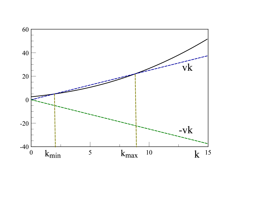
Once the values of are established, the k-integral in the region is straightforward, and we find
| (B.3) |
For the curve only intersects the straight line and only for , there is a minimum value of below which there is no further solution. This minimum value defines a threshold, at which . This behavior is displayed in fig. (4). For there is no longer intersection with the line, hence there is no solution for .
For the curve intersects both straight lines as shown in fig. (3).
Large limit:
The large limit of the spectral density can be extracted in a simple manner: in the original form, Eqn. (IV.11), we can neglect , furthermore, for large the delta function will be satisfied for large , therefore take , hence . Now the integrals are straightforward and yield the asymptotic limit
| (B.4) |
for .
Finding the roots for arbitrary values of and parameters in general must be done numerically, however, as discussed in the main text, the long time limit is determined by the small region of . Furthermore, we also focus on the “critical” region , as discussed above, this region is dominated by the emission and absorption of long wavelength phonons whose dispersion relation is . The equations that determine the intersections in this case simplify to,
| (B.5) |
and the acceptable solutions must correspond to .
It is convenient to introduce the following energy and momentum scales and Mach number ,
| (B.6) |
in terms of which we find the following solutions
A:)
i:) : Intersection with both branches ,
| (B.7) | |||||
| (B.8) |
ii:) : Intersection only with branch
| (B.9) | |||||
| (B.10) |
For the solutions (IV.40,IV.41) are only available for . This is evident from the expressions (B.9,B.10) in which the argument of the square roots are positive only for . This minimum value of determines a lower threshold for the spectral density at which at which point , therefore the region of negative for which the spectral density has support is given by
| (B.11) |
This threshold can also be understood from fig. (4): the dotted straight line becomes the tangent to the solid line (the curve ) when , which from the expressions (B.9,B.10) (in the long wavelength limit) corresponds to . For there are no further solutions and the spectral density vanishes.
B:)
There are no intersections for , there are solutions only for , these are given by ( only)
| (B.12) | |||||
| (B.13) |
For the “near critical” case and small , which is the relevant region for the long time dynamics, the spectral density simplifies substantially, we find in this case
| (B.14) |
Appendix C :
The asymptotic value is given by Eqn. (IV.33), with the definition of the spectral density, Eqn. (IV.11), the integral over yields,
| (C.1) |
Writing
| (C.2) |
the angular integral is straightforward. Introducing the following variables
| (C.3) |
we find
| (C.4) |
A closed form can be obtained for the equal mass case for which : changing variables to , we find in this case
| (C.5) |
Appendix D Long time behavior for :
As explained in the text, we first calculate the time dependent , and integrate back in time with the boundary condition that as . Introducing explicitly the lower threshold , it follows that the rate is given by
| (D.1) |
We now write , where only feature support for respectively, yielding
| (D.2) |
(a):
| (D.3) |
therefore
| (D.4) |
(b): write
| (D.5) |
and integrate by parts.
For the spectral density is analytic in as , it is given by
| (D.6) |
with and the dots stand for higher integer powers of . After integration by parts using (D.5), using the large and small behavior (B.4,D.6), respectively and subtracting , we find
| (D.7) |
(c): Use (D.5) to find
| (D.8) |
the first term yields
| (D.9) |
where we used that because for it follows from (B.9, B.10 ) that , therefore . Combining the above results for the contributions (a,b,c), we find
| (D.10) |
In the region near the upper limit , it is straightforward to find that the spectral density features an analytic power series expansion , hence upon rescaling this region yields inverse integer powers of : . In the region near the lower limit it follows from eqns. (B.9,B.10) and (B.14), that
| (D.11) |
therefore near threshold we find
| (D.12) |
where the dots stand for positive integer powers of . The first term in (D.11) yields the leading contribution from the region near threshold in the long time limit. The square root singularity at yields a fractional power of time in the long time limit, which is the leading asymptotic behavior. To see this insert (D.12) into the integral in (D.10) and rescale , the leading contribution to the integral (D) in the long-time limit becomes
| (D.13) |
with corrections which are higher inverse powers of . Now taking the limit in the integrals and carrying out the remaining integrals in we finally find
| (D.14) |
Gathering the results obtained above up to leading order we find
| (D.15) |
This result is valid for .
The next step is to integrate this result in time and append the asymptotic boundary condition. The integral in time of the oscillatory term cannot be found in a useful closed form, it being related to a Fresnel integral. However, progress can be made in the asymptotic long time limit with by writing
| (D.16) |
and integrating by parts, a process that can be iterated to yield
| (D.17) |
where the dots stand for higher powers of and the integration constant is fixed by the boundary condition in the asymptotic long time limit. Therefore, for we obtain
| (D.18) |
References
- (1) L. D. Landau, Phys. Z. Sowjetunion 3, 664 (1933) ( in L. Landau, Collected Papers, Gordon and Breach, New York, 67, (1965)).
- (2) S. I. Pekar, Zh. Eksper. Teor. Fiz. 16, 341 (1946).
- (3) T. D. Lee, F. E. Low, and D. Pines, Phys. Rev. 90, 297 (1953).
- (4) H. Frhlich, Advances in Physics, 3(11), 325 (1954); H. Frhlich, Proc. Royal Soc. A 215, 219 (1952).
- (5) R. P. Feynman, Phys. Rev., 97:660, (1955).
- (6) J. T. Devreese, Lectures at the International School of Physics Enrico Fermi, CLXI Course, ”Polarons in Bulk Materials and Systems with Reduced Dimensionality”, Varenna, Italy, 21.6. - 1.7.2005, arXiv:1611.06122
- (7) G. D. Mahan, Many Particle Physics, 2nd Ed., (Plenum Press, NY, 1990).
- (8) P. Massignan, M. Zaccanti, G. M. Bruun, Rep. Prog. Phys. 77, 034401 (2014).
- (9) I. Bloch, J. Dalibard, W. Zwerger, Rev. of Mod. Phys. 80, 885 (2008).
- (10) M. W. Zwierlein, A. Schirotzek, C. H. Schunck, and W. Ketterle, Science 311, 492 (2006)
- (11) M. W. Zwierlein, C. H. Schunck, A. Schirotzek, and W. Ketterle, Nature (London) 442, 54 (2006).
- (12) G. B. Partridge, W. Li, R. I. Kamar, Y. Liao, and R. G. Hulet, Science 311, 503 (2006).
- (13) A. Schirotzek, C.-H. Wu, A. Sommer, M. W. Zwierlein, Phys. Rev. Lett. 102, 230402 (2009).
- (14) C. Kohstall, M. Zaccanti, M. Jag, A. Trenkwalder, P. Massignan, G.M. Bruun, F. Schreck, and R. Grimm, Nature (London) 485, 615 (2012).
- (15) R. M. Kalas, D. Blume, Phys. Rev. A 73, 043608 (2006).
- (16) F. M. Cucchietti and E. Timmermans, Phys. Rev. Lett. 96, 210401 (2006).
- (17) J. Tempere, W. Casteels, M. K. Oberthaler, S. Knoop, E. Timmermans, and J. T. Devreese, Phys. Rev. B 80, 184504 (2013); W. Casteels, J. Tempere, J. T. Devreese, Phys. Rev.A83, 033631 (2011); W. Casteels, J. Tempere, J. T. Devreese, Phys. Rev.A86, 043614 (2012); W. Casteels, J. Tempere, J. T. Devreese, Phys. Rev.A84, 063612 (2011).
- (18) N. B. Jørgensen, L. Wacker, K. T. Skalmstang, M. M. Parish, J. Levinsen, R. S. Christensen, G. M. Bruun, J. J. Arlt, Phys. Rev. Lett. 117, 055302 (2016).
- (19) M.-G. Hu, M. J. Van de Graaff, D. Kedar, J. P. Corson, E. A. Cornell, D. S. Jin, Phys. Rev. Lett. 117, 055301, (2016).
- (20) R. S. Christensen, J. Levinsen, G. M. Bruun, Phys. Rev. Lett. 115, 160401 (2015).
- (21) Z. Z. Yun, Y. Ni, C. Robens, M. W. Zwierlein, arXiv:1904.02685.
- (22) F. Grusdt, E. Demler, arXiv:1510.04934.
- (23) S. Patrick Rath, R. Schmidt, Phys. Rev. A 88, 053632, (2013).
- (24) W. Casteels, M. Wouters, Phys. Rev. A 90, 043602 (2014).
- (25) E. Compagno, G. De Chiara, D. G. Angelakis, G. M. Palma, Scientific Reports 7, 2355 (2017).
- (26) J. Levinsen, M. M. Parish, G. M. Bruun Phys. Rev. Lett. 115, 125302, (2015).
- (27) L. A. Peña Ardila, S. Giorgini, Phys. Rev. A 92, 033612 (2015).
- (28) L. A. Peña Ardila, S. Giorgini Phys. Rev. A 94, 063640 (2016).
- (29) F. Grusdt, R. Schmidt, Y. E. Shchadilova, and E. Demler Phys. Rev. A 96, 013607 (2017).
- (30) S. M. Yoshida, S. Endo, J. Levinsen, M. M. Parish Phys. Rev. X 8, 011024 (2018).
- (31) A. Camacho-Guardian, G. M. Bruun Phys. Rev. X 8, 031042 (2018).
- (32) L. A. Peña Ardila, N. B. Jörgensen, T. Pohl, S. Giorgini, G. M. Bruun, J. J. Arlt, Phys. Rev. A 99, 063607 (2019).
- (33) Y. Ashida, R. Schmidt, L. Tarruell, E. Demler Phys. Rev. B 97, 060302(R) (2018).
- (34) I. N. Cherepanov, G. Bighin, L. Christiansen, A. Vestergaard Jorgensen, R. Schmidt, H. Sapelfeldt, M. Lemeshko, arXiv: 1906.12238; M. Lemeshko, Phys. Rev. Lett.118 095301 (2017); M. Lemeshko, R. Schmidt, arXiv: 1703.06753; X. Li, G. Bighin, E. Yakaboylu, M. Lemeshko, Molecular Physics 117, 1981 (2019).
- (35) A. G. Volosniev, H. W. Hammer, N. T. Zinner, Phys. Rev. A 92 023623 (2015).
- (36) A. Shashi, F. Grusdt, D. A. Abanin, E. Demler, Phys. Rev. A 89, 053617 (2014).
- (37) W. Li, S. Das Sarma, Phys.Rev.A90, 013618 (2014).
- (38) F. Chevy, Phys. Rev. A74, 063628 (2006).
- (39) Y. E. Shchadilova, R. Schmidt, F. Grusdt, E. Demler Phys. Rev. Lett. 117, 113002 (2016).
- (40) F. Grusdt, K. Seetharam, Y. Shchadilova, E. Demler Phys. Rev. A 97, 033612 (2018).
- (41) T. Lausch, A. Widera, M. Fleischhauer Phys. Rev. A 97, 023621 (2018).
- (42) K. K. Nielsen, L. A. Peña Ardila, G. M. Bruun, T. Pohl, New J. of Phys., 21, 043014 (2019).
- (43) M. Cetina, M. Jag, R. S. Lous, J. T.M. Walraven, R. Grimm, R. S. Christensen, and G. M. Bruun, Phys. Rev. Lett. 115, 135302 (2015).
- (44) M. Cetina,. M. Jag, R. S. Lous, I. Fritsche, J. T. M. Walraven, R. Grimm, J. Levinsen, M. M. Parish, R. Schmidt, M. Knap, E. Demler, Science 354, 96 (2016).
- (45) V. Weisskopf and E. Wigner, Z. Phys. 63, 54, (1930).
- (46) M. O. Scully, M. S.Zubairy, Quantum Optics, (Cambridge University Press, UK, 1997).
- (47) A. Goussev, R. A. Jalabert, H. M. Pastawski, D. Wisniacki, arXiv:1206.6348
- (48) T. Gorin, T. Prosen, T. H. Seligman, M. Znidaric, Phys. Rep. 435, 33 (2006).
- (49) M. A. Nielsen and I. L. Chuang. Quantum Computation and Quantum Information. (Cambridge University Press, Cambridge) (2001).
- (50) B. Misra, E.C.G. Sudarshan, J. Math. Phys. 18, 756 (1977); C.B. Chiu, B. Misra, E.C.G. Sudarshan, Phys. Rev. D16, 520 (1977); Phys. Lett. B117, 34 (1982).
- (51) H. Nakazato, M. Namiki, S. Pascazio, Int. J. Mod. Phys. B10, 247 (1996).
- (52) K. Koshino, A. Shimizu, Phys.Rept. 412, 191 (2005).
- (53) S. Pascazio, arXiv:1311.6645.
- (54) Wayne M. Itano, D. J. Heinzen, J. J. Bollinger, and D. J. Wineland Phys. Rev. A 41, 2295 (1990).
- (55) M. C. Fischer, B. Gutierrez-Medina, M. G. Raizen, Phys. Rev. Lett. 87,040402 (2001).
- (56) I. E. Mazets, G. Kurizki, N. Katz, and N. Davidson Phys. Rev. Lett. 94, 190403 (2005).
- (57) L. Fonda, G. C. Ghirardi, A. Rimini, Rep. Prog. Phys. 41, 587 (1978).
- (58) L. Maiani, M. Testa, Ann. of Phys. 263, 353 (1998); C. Bernardini, L. Maiani, M. Testa, Phys. Rev. Lett. 71, 2687 (1993).
- (59) P. Haikka, J. Goold, S. McEndoo, F. Plastina, S. Maniscalco, Phys. Rev. A 85, 060101(R) (2012).
- (60) F. M. Cucchietti, D. A. R. Dalvit, J. P. Paz, W. H. Zurek Phys. Rev. Lett. 91, 210403 (2003).
- (61) D. Boyanovsky, D. Jasnow, Phys. Rev. A 96, 062108 (2017).
- (62) S. I. Mistakidis, F. Grusdt, G. M. Koutentakis, P.Schmelcher, arXiv: 1907.06196.