MI-TH-1929
and the ANITA anomalous events in a three-loop neutrino mass model
Abstract
The most recent measurement of the fine structure constant leads to a 2.4 deviation in the electron anomalous magnetic moment -2, while the muon anomalous magnetic moment -2 has a long standing 3.7 deviation in the opposite direction. We show that these deviations can be explained in a three-loop neutrino mass model based on an Grand Unified Theory. We also study the impact such a model can have on the anomalous events observed by the ANITA experiment and find an insufficient enhancement of the event rate.
I Introduction
The Standard Model (SM) of particle physics, while a very successful and mathematically consistent theory, is challenged by a variety of experimental and theoretical puzzles. The neutrino oscillation data Fukuda et al. 1998; Ahmad et al. 2002 conclusively require neutrinos to have small but non-zero masses, and although a plethora of models exist in the literature for generating such masses, keeping the new dynamics at an energy scale accessible by current and near-future experiments proves nontrivial.
There are, additionally, some less certain but equally intriguing puzzles. One of the long-standing deviations of the experimental data from the theoretical predictions of the SM is the anomalous magnetic moment of the muon, . There is a 3.7 discrepancy between the experimental results Bennett et al. 2006; Tanabashi et al. 2018 and theoretical predictions Davier et al. 2017; Blum et al. 2018; Keshavarzi et al. 2018; Davier et al. 2019. This has recently been compounded with a 2.4 discrepancy between the experiment Hanneke et al. 2008; Hanneke et al. 2011 and theory Aoyama et al. 2018 values of . Moreover, the deviations are in opposite directions, meaning that the most straightforward Beyond the SM (BSM) explanations are insufficient. Also, does not follow the lepton mass scaling , which means that a model with new flavor structure in the leptonic sector would be required to explain the discrepancy.
Another interesting experimental result is the observation of the two up-going ultra-high energy cosmic ray air shower events by the ANITA Collaboration (ANtarctic Impulsive Transient Antenna) Gorham et al. 2016; Gorham et al. 2018. In principle, the events could be explained by a that up-scatters inside the Earth into a and then decays hadronically upon emergence. However, the Earth is far too opaque for both the neutrino and the charged lepton at the measured energy (about 0.6 EeV) and angle (about 30° below the horizon) Fox et al. 2018, requiring a neutrino flux that exceeds the current limits from the Pierre Auger Observatory Aab et al. 2015 and IceCube Aartsen et al. 2018.
From a big picture perspective, the unification of the electromagnetic and weak forces, the cancellation of gauge anomalies, and the near intersection of the gauge couplings at high energies in the SM all hint at a Grand Unified Theory (GUT). In a previous work, an GUT inspired model was shown to accommodate the neutrino masses and mixing parameters with TeV scale physics Dutta et al. 2018. Such a low scale was made possible by forbidding mass diagrams below 3-loop order. The flavor structure introduced in that work has the potential to explain the anomalies. In this work, we show that the scalar and fermionic degrees of freedom in that model together with the correct flavor structure can provide the necessary corrections to of both the muon and electron. We also study the implications on the ANITA observations and find that, while the expected event rate can be enhanced, explaining the two anomalous events remains challenging.
The outline of the paper is as follows: in Sec. II, we present the model. We define all the necessary physical fermions and scalar particles in Sec. III. In Sec. IV, we briefly discuss the neutrino mass generation. We study the for both electron and muon in Sec. V. In Sec. VI, we discuss the ANITA anomalous events. Finally, we conclude in Sec. VII.
II The Model from GUT
In this section, we briefly describe the gauge symmetry and the field content of the model introduced in Dutta et al. 2018. A maximal subgroup of is , while a maximal subgroup of is . We assume the latter is broken down to generate the SM gauge groups while the survives down to low energy and assumed not to affect the electric charge operator which retains the form . The particle content under is as follows
where , are the generation index. The fundamental representation of i.e. can accommodate , , , , , , , and , while the vector-like fermions and come from the 351 and representations of , respectively. The embedding of all fields in full GUT multiplets ensures that the gauge anomalies are automatically cancelled.
The scalar sector of the model has four scalar field with the following charge assignment
One representation can give , , and while one 650 gives the bi-doublet scalar field .
The most general renormalizable scalar potential is the following 11 1 We suppress the gauge indices and refer the reader to the previous work where this model was introduced Dutta et al. 2018.
| (1) |
where all the parameters are real and denotes a single contraction with an antisymmetric tensor.
The Yukawa potential is given by:
| (2) |
For simplicity, we assume . We impose a discrete symmetry such that only is odd under the symmetry while all the other particles are even. One implication of this symmetry is that the and terms in Eq. 2 are forbidden. The lightest component of is therefore stable and may contribute to the dark matter density.
III The physical scalars and fermions
We define the physical scalar particles and fermions in the mass basis necessary for the calculations in this section. The total number of scalar degrees of freedom is 24, out of which 6 are eaten by the massive gauge bosons. This leaves us with 18 physical scalars. After the spontaneous symmetry breaking the Higgs scalars acquire vacuum expectation values (vevs) and we can write them as
where the vev of () is (10-100) TeV and breaks the symmetry, while the vevs of and ( and respectively) are (10-100) GeV and break the electroweak gauge symmetry.
The charged states and will mix with a mixing angle and give the charged physical scalars and respectively with masses and
| (11) |
where . Similarly, four more charged physical scalars and with masses and respectively can arise from the mixing of and
| (12) |
There is a total of five neutral CP even states, out of which , and will mix resulting in three physical neutral scalars , and with masses , , and , respectively. We identify the as the SM physical Higgs field, with mass . The fields in the mass basis, are related to those in the interaction basis, by a rotation matrix which can be parametrized with three angle as follows
| (13) |
where , and (). We can parametrize the mixing of three neutral CP-odd states, , , and in a similar way with , and the three angles are denoted as . We only get one physical neutral pseudoscalar with mass . The interaction states can be written as, , , and .
The rest of the two neutral CP-even states and give one physical neutral scalar with mass . The mixing matrix can be parametrize by an angle as
| (14) |
The interaction states can be written as and . Similar mixing happens between the two neutral CP-odd states and . We parametrize the mixing matrix with an angle . One physical pseudoscalar with mass is generated. In terms of this physical pseudoscalar, we write and .
For the purpose of calculating the contributions to the anomalous magnetic moment and the ANITA observations, the relevant terms from Eq. 2 can be written as follows
| (15) |
where are neutral components of and (see Eq. III). The vector-like leptons and mix and give rise to two charged physical vector-like leptons given by,
| (16) |
respectively with masses and , where the mixing angle, , can be determined by diagonalizing the mass matrix. We summarize all the relevant fields in Table 1.
| Particle type | Particles | Mass parameters | Mass values | Possible final states at LHC | ||||||||
| Charged scalars | GeV |
| ||||||||||
|
| |||||||||||
| Neutral scalars |
|
|
|
| ||||||||
| Neutral pseudoscalar | (500) GeV |
| ||||||||||
| Charged vector-like leptons | GeV |
| ||||||||||
| Neutral vector-like leptons | GeV |
| ||||||||||
| New gauge bosons | TeV |
| ||||||||||
| Charged vector-like quark | (1) TeV |
|
IV Neutrino masses
Here we summarize the neutrino mass generation mechanism and the numerical results in our model, and refer the reader to Dutta et al. 2018 for more details.
The tree-level Lagrangian in our model contains no mass terms for neutrinos, so one must rely on radiative mass generation (i.e. through loops). Normally, the particles running in such loops need to be made heavy to achieve the vanishingly small neutrino masses, but due to the particle content and the associated symmetry, the Majorana neutrino mass in our model cannot be generated below the three-loop level. The dimension-5 effective Majorana neutrino mass operator , where is some effective mass scale, can be realized at the three-loop level as shown in Fig. 1. The new heavy gauge bosons and play an important role in making the neutrino mass values small, and the mass matrix also gets suppressed from the loop factor . Due to all these suppressions, the new physics associated with the tiny neutrino masses can be kept at the TeV scale.

Based on the benchmark points determined in Dutta et al. 2018, the following parameter point can generate the correct neutrino observables
| (17) |
Renormalization group evolution suggest that the gauge coupling is of similar strength to the SM couplings, and we fixed it to be 0.35. Note that in Dutta et al. 2018, the value of tan was set to be 2 in exchange for a smaller value of (the parametric dependence of the neutrino mass matrix is ). Since we will later need large Yukawa couplings to explain the magnetic moments, we have altered the original benchmark point while maintaining the neutrino masses. For the remainder of the paper we assume parameters in the neighborhood of this benchmark point.
The particle spectrum is consistent with the LHC as shown in Dutta et al. 2018. Of particular importance is that the new leptons can be abundantly produced at the LHC, but all of their decays include neutral states that are almost degenerate in mass making them extremely difficult to find in missing energy searches. This holds true for all fields in our model that are within the energy reach of the LHC and could, in principle, be subject to such constraints.
V The Muon and Electron Anomalous Magnetic Moments
V.I Background
As mentioned in the Introduction, there is a 3.7 discrepancy between the experimental results Bennett et al. 2006; Tanabashi et al. 2018 and the theoretical predictions Davier et al. 2017; Blum et al. 2018; Keshavarzi et al. 2018; Davier et al. 2019 of the anomalous magnetic moment of the muon, . The discrepancy was found to be
| (18) |
The precision of the SM prediction will be improved in the future Lehner et al. 2019. An updated measurement is expected soon from Fermilab Grange et al. 2015; Fienberg 2019 and J-PARC Saito 2012.
On the other hand, the direct experimental measurement of the electron anomalous magnetic moment, Hanneke et al. 2008, had been in agreement with the SM prediction, Aoyama et al. 2018, at the level of 1.7 until recently, when an updated value of the fine structure constant has been measured with high precision using Cesium atoms Parker et al. 2018
| (19) |
The result of this precise measurement of leads to a 2.4 discrepancy between the experiment Hanneke et al. 2008; Hanneke et al. 2011 and theory Aoyama et al. 2018 values of
| (20) |
The simplest BSM explanations of these values, say a new mediator that couples to both electrons and muons, are expected to result in and of the same sign, since the new physics couplings would appear twice in each diagram. Moreover, if coupling universality is assumed then we additionally expect the corrections to scale with the lepton mass, that is . Since neither of those is true, a more complex solution is needed. Several such solutions exist in the literatures Davoudiasl and Marciano 2018; Crivellin et al. 2018; Liu et al. 2019; Dutta and Mimura 2019; Han et al. 2019; Crivellin and Hoferichter 2019; Endo and Yin 2019.
In this work, we rely on the diversity of Yukawa couplings in Eq. 15. These terms allow for a variety of new scalars and fermions to run in the loop, with couplings that are both chiral (different for left-handed and right-handed components) and flavor non-universal (different for each lepton). As we show in the next subsection, the chirality of these interactions leads certain couplings to appear only once in a given diagram thereby allowing for corrections to and in opposite directions, while the non-universality allows for modifying each independently of the other.
V.II Calculations and results
We now proceed to present the calculations and results of the anomalous magnetic moments. We choose to work in the physical mass basis. Upon expanding Eq.15 in terms of the physical fields, the Lagrangian that generates the necessary one-loop diagrams can be written as
| (21) | |||||
where the coefficients are given by
| (22) |
The 11 different terms in Eq. 21 can generate 11 different Feynman diagrams as shown in Fig. 2 22 2 We have used the package TikZ-Feynman Ellis 2017 to draw the diagrams.. Note that the couplings - are linear combinations of three Yukawa couplings , , and . This will lead to products of two different Yukawa couplings in various diagrams.


The Feynman diagrams of Fig. 2 can be broadly categorized into two category: ones with a neutral scalar inside the loop and ones with a charged scalar. Each term in the above Lagrangian takes the general form
| (23) |
where denotes the fermion and the scalar that run in the loop.
Following Ref. Leveille 1978, the contribution from the first type of diagrams with a neutral scalar can be written as
| (24) |
and the contribution of the second type of diagrams with charged scalar can be written as
| (25) |
In the following, we discuss the various contributions to .
- •
The first four terms of Eq. 21 give four diagrams where we have the vector-like leptons and the new neutral scalar particles inside the loop. Fig. 2(a) shows these diagrams and their contributions to is given by Eq. 24. From Eq. V.II and Eq. 24, we get quadratic terms in the Yukawa couplings () as well as cross terms (, and ). The quadratic terms are proportional to while the cross terms are proportional to . With a fermion mass GeV, the cross terms of Yukawa couplings can lead to contributions that are both large and of opposite signs for the muon and electron cases.
- •
The next three terms of Eq. 21 give three more diagrams in Fig. 2(b) with the new neutral scalars inside the loop along with the SM muons and electrons. Together with the Hermitian conjugates, these terms become simple, for example, . Their contributions to is given by Eq. 24. All the diagrams are proportional to the SM Yukawa couplings, , and hence suppressed by . Therefore, their contribution to is small compared to the first four diagrams. Since we do not rely on these contributions, the masses of the scalars involved are thus far not fixed.
- •
Fig. 2(c) and 2(d) give four more diagrams arising from the last four terms in Eq. 21. All four diagrams have charged scalars and neutral fermions such as inside the loop. Their contributions to are given in Eq. 25. These diagrams are also suppressed compared to the diagrams with cross terms due to the SM Yukawa factors . Additionally, since these particles also enter into the three-loop diagrams (Fig. 1) needed for neutrino mass generation, their masses are already fixed in our model, and so they do not play important roles in the calculations.
- •
In addition to these 11 scalar loop diagrams contributing to , we do get contributions from the gauge bosons associated with the new gauge group . The lower limit on the new gauge boson masses is 3.6 TeV Sirunyan et al. 2018; Aaboud et al. 2017; Dutta et al. 2018 assuming the gauge coupling is 0.35. These diagrams are also suppressed by the square of lepton masses. Therefore, these diagrams are small compared to the scalar diagrams of Fig. 2(a) and their contributions can be neglected.
For completeness we consider the contributions to from all the scalar diagrams. The total contribution to can be expressed in a simple form
| (26) | |||||
In order to find a working parameter point, we begin by fixing the dimensionless parameters that are not yet set by neutrino masses and then vary the masses of new fields. The ’s are fixed by the SM charged lepton masses by the relation , and we therefore set them to be , and . Other necessary coupling constants can be taken as follows: .
For simplicity, we choose the mixing angles , , and to be . In Table 2, we give five different sets of values of the fermion and scalar masses that play an important role in the and calculations. As we discussed earlier, the dominant contributions to are coming mainly from the diagrams of Fig. 2(a), in particular from the terms with the product of two different Yukawa couplings. This Yukawa structure allows for the sought after violation of the scaling dependance , leading instead to a ratio of and without a constraint on the sign. The particles necessary to produce this dominant contributions are , and . This is true for any value of the parameters in Eq. IV.
| Benchmark Point | (GeV) | (GeV) | (GeV) | (GeV) |
|---|---|---|---|---|
| BP1 | 120 | 121 | 350 | 1985 |
| BP2 | 120 | 135 | 350 | 1121 |
| BP3 | 120 | 102 | 350 | 1578 |
| BP4 | 120 | 118 | 350 | 570 |
| BP5 | 120 | 145 | 350 | 2150 |
In order to get of sense of how readily the model fits the observations we perform a random scan over some of the parameters going into the calculation. We limit the scan to a subset of four parameters for tractability. The diagrams in Fig. 2 suggest that the dependence on and is similar to that on and respectively. We, therefore, fix the former and scan over the latter. We similarly choose to fix and vary .
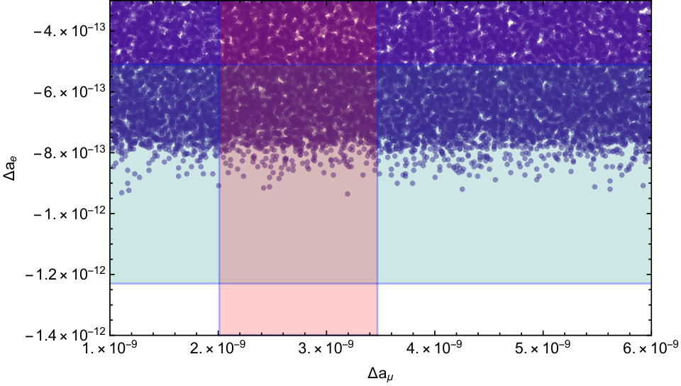
We sample 100,000 points at random from the range shown in Table 3 with = 0.9, = 0.5,= 120 GeV and = 350 GeV. In Fig. 3 we show the results as a scatter plot in the plane along with the 1 bands of Eqs. 18 and 20 ( and ). About 2800 points fell into the intersection of the two bands. We can see that while a wide range of can be achieved, the values of mostly lie on the upper end of the band.
In experimenting with other scanning schemes we find that, indeed, allowing for the fixed parameters to vary leads to no significant expansion of the reach. We also find that there is very strong dependence on the value of . Namely, expanding the lower scan limit of down to 0.01 leads to a dramatic drop in the density of viable points.
| Parameter | Range |
|---|---|
| 0.6-3.0 | |
| 0.001-2.0 | |
| 100-150 GeV | |
| 300-2500 GeV |
VI Anita
VI.I Background
ANITA is an Antarctic balloon experiment that looks for ultra high energy cosmic rays by detecting the associated geosynchrotron emissions using a series of radio antennas Gorham et al. 2009. The flight altitude of over 30 km leads to a coverage of the Antarctic ice which compensates for the limited operation time compared to IceCube and the Pierre Auger Observatory, and offers sensitivity to a complementary range of energies and phenomena. In particular, the polarity of the geosynchroton radiation is correlated with the Earth’s magnetic field, allowing ANITA to discriminate between showers emerging directly from the Earth and down going showers that are reflected off the ice. During the first and third flights of ANITA, 2 out of the 36 detected events stood out.
During its first flight, ANITA-I Gorham et al. 2016, an event with an energy of 0.60.4 EeV was detected at a zenith angle of with a non-inverted polarity, suggesting that the event emerged from the Earth rather than reflected off the ice. More recently, a similar event, with non-inverted polarity, has been found in the ANITA-III data Gorham et al. 2018, with an energy of 0.56 EeV and a zenith angle of . At such high energies the survivability of neutrinos passing through such a long arc length within the Earth is very low, and the isotropic neutrino flux required to explain the events with a that up-scatters to a has been found to be at least 2 Romero-Wolf et al. 2019, and possibly 6 Fox et al. 2018 orders of magnitude larger than the limits set by the Pierre Auger Observatory and IceCube. The emergence probability has also been studied in Alvarez-Muñiz et al. 2018
One approach around this is to replace the with an intermediary field with a long lifetime and large survivability in matter which decays to a upon or right before emergence. In our case, we rely on the new neutral field which is produced via the scattering of a off of the Earth matter. The new heavy field can then propagate through the Earth, emerge at the South Pole, and generate a as part of its decay products, which can then decay hadronicaly leading to an observable signal at ANITA. A similar approach has been considered in Huang 2018; Dudas et al. 2018; Connolly et al. 2018; Collins et al. 2019; Chauhan and Mohanty 2019; Bhupal Dev 2019.
There are, however, several caveats to the story. It has been shown that solutions that rely on a neutrino flux still exceed the astrophysical bounds despite the higher rate of emergence compared to the SM only scenario (see, for example, Cline et al. 2019). This is true for an isotropic neutrino flux or a long-lasting point source, so one needs to postulate a rather exotic astrophysical source of neutrinos to fully explain the ANITA observation. Explanations that rely on a source other than a neutrino flux, say dark matter, do not suffer from this drawback Anchordoqui et al. 2018; Yin 2019; Heurtier et al. 2019a; Heurtier et al. 2019b; Hooper et al. 2019; Cline et al. 2019; Esteban et al. 2019; Heurtier et al. 2019b; Borah et al. 2019, although see the discussion in Ref. Chipman et al. 2019. A summary of feasibility of various approaches can be found in the conference proceedings by Ref. Anchordoqui et al. 2019.
A second caveat is that any BSM explanation of the ANITA events will have to confront the lack of similar events in IceCube Fox et al. 2018. Depending on the mechanism utilized, the dynamics could conspire to produce a signal in one experiment but not the other. Intriguingly, building upon a proposal by Ref. Kistler and Laha 2018, Ref. Fox et al. 2018 shows that a small reported tension between the northern track and the full sky spectra measured by IceCube could be alleviated if some of the up-going muon events are interpreted as misidentified tau events, and they identify three such events by calculating the probability of emergence as a function of energy and angle. If true, these events would have higher energy than reported by IceCube, thus adding support to the ANITA observations. This interpretation, however, does not improve the viability of a neutrino flux explanation at either experiment.
A final caveat is that non-BSM explanations of the ANITA observations are still possible. Very recently it was proposed that an additional electromagnetic component can be emitted during the shower’s transit across the ice surface with a non-inverted polarity de Vries and Prohira 2019. Another recent paper proposed that some ice features can lead to reflection without an inversion of polarity Shoemaker et al. 2019. Two earlier proposals that were not able to account for the anomaly were transition radiation through the air Motloch et al. 2017 and a more accurate treatment of the reflections of the electromagnetic waves Dasgupta and Jain 2018.
With all of that mind, we content ourselves with an estimate of the emergence fraction of taus in our model, using the SM fraction from Fox et al. 2018 as a reference point.
VI.II Calculations and results
To enhance the rate of emergence, we identify a particle that can be produced from neutrino scattering off of nuclei, survive passage through Earth along a chord length of about 5740-7210 km corresponding to the angles of two ANITA events, and decay to a lepton. The neutral vector-like lepton from the doublet can serve such a purpose. It can be produced in the -nucleon scattering mediated by the neutral scalars along with a heavy quark as shown in Fig. 4(a). It can then propagate through the Earth without significant attenuation and finally decay into a lepton pair and another heavy neutral particle as shown in Fig. 4(b).
We start our analysis by writing the necessary terms of the Lagrangian in the mass basis
| (27) |
The first four terms of Eq. 27 are needed for the neutrino-nucleon cross sections and the rest of the terms are responsible for the decay of . The Feynman diagrams of the scattering process and decay channel in the mass basis are shown in Fig. 4(a) and Fig. 4(b), respectively.


We consider cosmic neutrinos of energies about (EeV) which scatter off of matter producing along with hadrons. In the limit of large momentum transfer the differential cross section is given by
| (28) |
where is the momentum transfer, and and are the parton distribution functions (pdf) of the quarks and anti-quarks, respectively. is the nucleon mass, is the incoming neutrino energy, while and are dimensionless variables defined as
| (29) |
where is the energy loss in the laboratory frame. The momentum transfer is always greater than the nucleon mass. is the fractions of the initial neutrino energy transferred to the hadrons. The total cross section can be obtained by integrating Eq. 28 over and
| (30) |
where , and is determined by the relation as . The total cross section in Eq. 30 can be calculated numerically with the given input parameters of the model and the pdfs of the quarks and antiquarks. We use the CTEQ5 parton distribution Lai et al. 2000 in our numerical calculations. We also cross checked our calculations against the analytical form of the pdfs Berger et al. 2007 and found agreement. The cross sections corresponding to three different benchmark points are shown in Table 4. The coupling constants are taken to be and . The cross section in Eq. 28 is sensitive to the mixing angles and . These angles also appear in the calculations but Eq. 26 is not sensitive enough to these angles to change the numerical results. Therefore we can vary them to get different cross sections from Eq. 30. We choose three different values of , and , and corresponding to the three Benchmark Points in Table 4.
The produced in the collision propagates through the Earth and eventually decays dominantly into lepton pair and . The three-body decay channel is mediated by the neutral scalars and . The decay width is given by
| (31) |
where
| (32) |
| (33) |
Eq. 31 gives the sum over all four contributions for and . The same decay channel is open for all charged leptons and down type quarks in the SM. We choose and such that the bottom quark final state is kinematically forbidden. The decays to muons and strange quarks are suppressed by a factor 100 due to the SM Yukawas. The lifetime of in the rest frame is , where is the total decay width of . Note that the masses of the new scalar fields are set to be (500) GeV, making their contributions to the decay width sub-leading compared to that of the SM Higgs. We show the lifetime for a few benchmark points in Table 4, taking the coupling constants to be and .
Let us now define the survival probability of emergence, . We follow closely the treatment in Ref. Collins et al. 2019. We assume that a fraction of neutrinos has survived the SM interactions after propagating a distance of km. We take the SM interaction length to be km Fox et al. 2018. These surviving neutrinos can produce as a result of the collision with nucleons inside the Earth. The interaction length of the -nucleon scattering process can be defined as , where is the scattering cross section, is the Avogadro number, and is the density of target material. For simplicity, we assume the Earth to have uniform density and take the value to be gm/cm3. The then travels a distance of km, where 6475 km is the average chord length along the Earth corresponding to the two ANITA events, and finally decays below an altitude of about 10 km, otherwise the air shower will not get a chance to fully develop Collins et al. 2019. The decay length in the Earth frame is . We can now define the survival probability as
| (34) | |||||
where from right to left, the first expression is the fraction of s that survive passage through matter until the interaction point, , where is produced. The second factor is the fraction of neutrinos converted to anywhere inside the Earth between the emergence point and the entire chord length . The third factor is the fraction of those that decay after a sufficient distance to emerge from the Earth, and a further distance, , beyond which it would exceed the 10 km altitude. We take km. The fourth expression is the fraction of that decays into hadrons within the distance 20 km. The decay length of is , where the lifetime of is 0.3 s and the branching ratio of to hadrons is 0.65 Tanabashi et al. 2018.
We dial our parameters such that both and are comparable to the chord length. The corresponding scattering cross section, lifetime and the estimated survival probability are shown in Table 4. The expression above could yield a higher value if we choose a much shorter and longer , but then one must account for the probability of regeneration. The interaction length of regeneration is similar to at such energies, and once accounted for the gains from reducing are countered and one gets similar values of . For comparison, the SM survivability found by Fox et al. 2018 are and for the ANITA-I and ANITA-III events respectively at EeV. Note that the results in Table 4 are far less sensitive to the chord length compared to the survivability in the SM.
| Point | (pb) | (ns) | (km) | (km) | ||||||||||
| BP1 | 500 | 1200 | 125 | 500 | 500 | 500 | 1000 | 105 | 110 | 708 | 2 | 4705 | 6387 | |
| BP2 | 500 | 600 | 125 | 400 | 400 | 500 | 1000 | 110 | 115 | 887 | 2 | 3757 | 6368 | |
| BP3 | 600 | 800 | 125 | 500 | 600 | 800 | 1000 | 115 | 120 | 1066 | 2 | 3126 | 6350 |
VII Conclusion
We were able to explain the observed values of the anomalous magnetic moments of the muon and electron within the framework of an inspired GUT model. In addition to the theoretical appeal of fitting into a unification picture, the model has been shown in an earlier work to generate neutrino masses radiatively at the 3-loop level, thereby allowing for the new physics mass scale to be within the reach of the current and proposed collider experiments. The flavor structure of the model, which allowed the neutrino fit, played a crucial role to explain the anomalous magnetic moments of the muon and electron. In this model, the ratio of and is proportional to with a relative sign difference between them as required by the experiments. We have also studied the model’s contribution to the anomalous events observed by the ANITA experiments using the mass scale of new physics set by the neutrino fitting and found a modest improvement over the SM predictions.
We stress that in explaining all the aforementioned observations we have introduced various new, SM charged particles in the 100 GeV to 1 TeV range. The primary reason these have not been ruled out is that they are too mass degenerate with one of their decay products to be covered by existing LHC searches. This adds to the list of motivations of why the efforts put in closing this mass gap in collider searches are worth pursuing.
Acknowledgments
MA, BD, and SG are supported in part by the DOE Grant No. DE-SC0010813. TL is supported in part by the Projects 11647601 and 11875062 supported by the National Natural Science Foundation of China, and by the Key Research Program of Frontier Science, CAS.
References
- Fukuda et al. (1998) Y. Fukuda et al. (Super-Kamiokande), Phys. Rev. Lett. 81, 1562 (1998), arXiv:hep-ex/9807003 [hep-ex] .
- Ahmad et al. (2002) Q. R. Ahmad et al. (SNO), Phys. Rev. Lett. 89, 011301 (2002), arXiv:nucl-ex/0204008 [nucl-ex] .
- Bennett et al. (2006) G. W. Bennett et al. (Muon g-2), Phys. Rev. D73, 072003 (2006), arXiv:hep-ex/0602035 [hep-ex] .
- Tanabashi et al. (2018) M. Tanabashi et al. (Particle Data Group), Phys. Rev. D98, 030001 (2018).
- Davier et al. (2017) M. Davier, A. Hoecker, B. Malaescu, and Z. Zhang, Eur. Phys. J. C77, 827 (2017), arXiv:1706.09436 [hep-ph] .
- Blum et al. (2018) T. Blum, P. A. Boyle, V. Gülpers, T. Izubuchi, L. Jin, C. Jung, A. Jüttner, C. Lehner, A. Portelli, and J. T. Tsang (RBC, UKQCD), Phys. Rev. Lett. 121, 022003 (2018), arXiv:1801.07224 [hep-lat] .
- Keshavarzi et al. (2018) A. Keshavarzi, D. Nomura, and T. Teubner, Phys. Rev. D97, 114025 (2018), arXiv:1802.02995 [hep-ph] .
- Davier et al. (2019) M. Davier, A. Hoecker, B. Malaescu, and Z. Zhang, (2019), arXiv:1908.00921 [hep-ph] .
- Hanneke et al. (2008) D. Hanneke, S. Fogwell, and G. Gabrielse, Phys. Rev. Lett. 100, 120801 (2008), arXiv:0801.1134 [physics.atom-ph] .
- Hanneke et al. (2011) D. Hanneke, S. F. Hoogerheide, and G. Gabrielse, Phys. Rev. A83, 052122 (2011), arXiv:1009.4831 [physics.atom-ph] .
- Aoyama et al. (2018) T. Aoyama, T. Kinoshita, and M. Nio, Phys. Rev. D97, 036001 (2018), arXiv:1712.06060 [hep-ph] .
- Gorham et al. (2016) P. W. Gorham et al. (ANITA), Phys. Rev. Lett. 117, 071101 (2016), arXiv:1603.05218 [astro-ph.HE] .
- Gorham et al. (2018) P. W. Gorham et al. (ANITA), Phys. Rev. Lett. 121, 161102 (2018), arXiv:1803.05088 [astro-ph.HE] .
- Fox et al. (2018) D. B. Fox, S. Sigurdsson, S. Shandera, P. Mészáros, K. Murase, M. Mostafá, and S. Coutu, Submitted to: Phys. Rev. D (2018), arXiv:1809.09615 [astro-ph.HE] .
- Aab et al. (2015) A. Aab et al. (Pierre Auger), Phys. Rev. D91, 092008 (2015), arXiv:1504.05397 [astro-ph.HE] .
- Aartsen et al. (2018) M. G. Aartsen et al. (IceCube), Phys. Rev. D98, 062003 (2018), arXiv:1807.01820 [astro-ph.HE] .
- Dutta et al. (2018) B. Dutta, S. Ghosh, I. Gogoladze, and T. Li, Phys. Rev. D98, 055028 (2018), arXiv:1805.01866 [hep-ph] .
- Lehner et al. (2019) C. Lehner et al. (USQCD), (2019), arXiv:1904.09479 [hep-lat] .
- Grange et al. (2015) J. Grange et al. (Muon g-2), (2015), arXiv:1501.06858 [physics.ins-det] .
- Fienberg (2019) A. T. Fienberg (Muon g-2), in 54th Rencontres de Moriond on QCD and High Energy Interactions (Moriond QCD 2019) La Thuile, Italy, March 23-30, 2019 (2019) arXiv:1905.05318 [hep-ex] .
- Saito (2012) N. Saito (J-PARC g-’2/EDM), Proceedings, International Workshop on Grand Unified Theories (GUT2012): Kyoto, Japan, March 15-17, 2012, AIP Conf. Proc. 1467, 45 (2012).
- Parker et al. (2018) R. H. Parker, C. Yu, W. Zhong, B. Estey, and H. Müller, Science 360, 191 (2018), arXiv:1812.04130 [physics.atom-ph] .
- Davoudiasl and Marciano (2018) H. Davoudiasl and W. J. Marciano, Phys. Rev. D98, 075011 (2018), arXiv:1806.10252 [hep-ph] .
- Crivellin et al. (2018) A. Crivellin, M. Hoferichter, and P. Schmidt-Wellenburg, Phys. Rev. D98, 113002 (2018), arXiv:1807.11484 [hep-ph] .
- Liu et al. (2019) J. Liu, C. E. M. Wagner, and X.-P. Wang, JHEP 03, 008 (2019), arXiv:1810.11028 [hep-ph] .
- Dutta and Mimura (2019) B. Dutta and Y. Mimura, Phys. Lett. B790, 563 (2019), arXiv:1811.10209 [hep-ph] .
- Han et al. (2019) X.-F. Han, T. Li, L. Wang, and Y. Zhang, Phys. Rev. D99, 095034 (2019), arXiv:1812.02449 [hep-ph] .
- Crivellin and Hoferichter (2019) A. Crivellin and M. Hoferichter, in 33rd Rencontres de Physique de La Vallée d’Aoste (LaThuile 2019) La Thuile, Aosta, Italy, March 10-16, 2019 (2019) arXiv:1905.03789 [hep-ph] .
- Endo and Yin (2019) M. Endo and W. Yin, (2019), arXiv:1906.08768 [hep-ph] .
- Ellis (2017) J. Ellis, Comput. Phys. Commun. 210, 103 (2017), arXiv:1601.05437 [hep-ph] .
- Leveille (1978) J. P. Leveille, Nucl. Phys. B137, 63 (1978).
- Sirunyan et al. (2018) A. M. Sirunyan et al. (CMS), JHEP 08, 130 (2018), arXiv:1806.00843 [hep-ex] .
- Aaboud et al. (2017) M. Aaboud et al. (ATLAS), Phys. Rev. D96, 052004 (2017), arXiv:1703.09127 [hep-ex] .
- Gorham et al. (2009) P. W. Gorham et al. (ANITA), Astropart. Phys. 32, 10 (2009), arXiv:0812.1920 [astro-ph] .
- Romero-Wolf et al. (2019) A. Romero-Wolf et al., Phys. Rev. D99, 063011 (2019), arXiv:1811.07261 [astro-ph.HE] .
- Alvarez-Muñiz et al. (2018) J. Alvarez-Muñiz, W. R. Carvalho, A. L. Cummings, K. Payet, A. Romero-Wolf, H. Schoorlemmer, and E. Zas, Phys. Rev. D97, 023021 (2018), [erratum: Phys. Rev.D99,no.6,069902(2019)], arXiv:1707.00334 [astro-ph.HE] .
- Huang (2018) G.-y. Huang, Phys. Rev. D98, 043019 (2018), arXiv:1804.05362 [hep-ph] .
- Dudas et al. (2018) E. Dudas, T. Gherghetta, K. Kaneta, Y. Mambrini, and K. A. Olive, Phys. Rev. D98, 015030 (2018), arXiv:1805.07342 [hep-ph] .
- Connolly et al. (2018) A. Connolly, P. Allison, and O. Banerjee, (2018), arXiv:1807.08892 [astro-ph.HE] .
- Collins et al. (2019) J. H. Collins, P. S. Bhupal Dev, and Y. Sui, Phys. Rev. D99, 043009 (2019), arXiv:1810.08479 [hep-ph] .
- Chauhan and Mohanty (2019) B. Chauhan and S. Mohanty, Phys. Rev. D99, 095018 (2019), arXiv:1812.00919 [hep-ph] .
- Bhupal Dev (2019) P. S. Bhupal Dev, (2019), arXiv:1906.02147 [hep-ph] .
- Cline et al. (2019) J. M. Cline, C. Gross, and W. Xue, (2019), arXiv:1904.13396 [hep-ph] .
- Anchordoqui et al. (2018) L. A. Anchordoqui, V. Barger, J. G. Learned, D. Marfatia, and T. J. Weiler, LHEP 1, 13 (2018), arXiv:1803.11554 [hep-ph] .
- Yin (2019) W. Yin, Proceedings, 20th International Symposium on Very High Energy Cosmic Ray Interactions (ISVHECRI 2018): Nagoya, Japan, May 21-25, 2018, EPJ Web Conf. 208, 04003 (2019), arXiv:1809.08610 [hep-ph] .
- Heurtier et al. (2019a) L. Heurtier, Y. Mambrini, and M. Pierre, Phys. Rev. D99, 095014 (2019a), arXiv:1902.04584 [hep-ph] .
- Heurtier et al. (2019b) L. Heurtier, D. Kim, J.-C. Park, and S. Shin, (2019b), arXiv:1905.13223 [hep-ph] .
- Hooper et al. (2019) D. Hooper, S. Wegsman, C. Deaconu, and A. Vieregg, (2019), arXiv:1904.12865 [astro-ph.HE] .
- Esteban et al. (2019) I. Esteban, J. Lopez-Pavon, I. Martinez-Soler, and J. Salvado, (2019), arXiv:1905.10372 [hep-ph] .
- Borah et al. (2019) D. Borah, A. Dasgupta, U. K. Dey, and G. Tomar, (2019), arXiv:1907.02740 [hep-ph] .
- Chipman et al. (2019) S. Chipman, R. Diesing, M. H. Reno, and I. Sarcevic, (2019), arXiv:1906.11736 [astro-ph.HE] .
- Anchordoqui et al. (2019) L. A. Anchordoqui et al. (2019) arXiv:1907.06308 [hep-ph] .
- Kistler and Laha (2018) M. D. Kistler and R. Laha, Phys. Rev. Lett. 120, 241105 (2018), arXiv:1605.08781 [astro-ph.HE] .
- de Vries and Prohira (2019) K. D. de Vries and S. Prohira, (2019), arXiv:1903.08750 [astro-ph.HE] .
- Shoemaker et al. (2019) I. M. Shoemaker, A. Kusenko, P. K. Munneke, A. Romero-Wolf, D. M. Schroeder, and M. J. Siegert, (2019), arXiv:1905.02846 [astro-ph.HE] .
- Motloch et al. (2017) P. Motloch, J. Alvarez-Muñiz, P. Privitera, and E. Zas, Phys. Rev. D95, 043004 (2017), arXiv:1606.07059 [astro-ph.HE] .
- Dasgupta and Jain (2018) P. Dasgupta and P. Jain, (2018), arXiv:1811.00900 [physics.class-ph] .
- Lai et al. (2000) H. L. Lai, J. Huston, S. Kuhlmann, J. Morfin, F. I. Olness, J. F. Owens, J. Pumplin, and W. K. Tung (CTEQ), Eur. Phys. J. C12, 375 (2000), arXiv:hep-ph/9903282 [hep-ph] .
- Berger et al. (2007) E. L. Berger, M. M. Block, and C.-I. Tan, Phys. Rev. Lett. 98, 242001 (2007), arXiv:hep-ph/0703003 [HEP-PH] .