Total variation based community detection using a nonlinear optimization approach
Andrea Cristofari∗, Francesco Rinaldi∗, Francesco Tudisco†
∗Department of Mathematics “Tullio Levi-Civita”
University of Padua
Via Trieste 63, 35121 Padua (Italy)
E-mail: andrea.cristofari@unipd.it, rinaldi@math.unipd.it
†Gran Sasso Science Institute
Viale F. Crispi 7, 67100 L’Aquila (Italy)
E-mail: francesco.tudisco@gssi.it
Abstract. Maximizing the modularity of a network is a successful tool to identify an important community of nodes. However, this combinatorial optimization problem is known to be NP-complete. Inspired by recent nonlinear modularity eigenvector approaches, we introduce the modularity total variation and show that its box-constrained global maximum coincides with the maximum of the original discrete modularity function. Thus we describe a new nonlinear optimization approach to solve the equivalent problem leading to a community detection strategy based on . The proposed approach relies on the use of a fast first-order method that embeds a tailored active-set strategy. We report extensive numerical comparisons with standard matrix-based approaches and the Generalized RatioDCA approach for nonlinear modularity eigenvectors, showing that our new method compares favourably with state-of-the-art alternatives.
Keywords. Community detection. Graph modularity. Total variation. Nonlinear optimization. Active-set method.
MSC2000 subject classifications. 49M20. 65K10. 91D30. 91C20.
1 Introduction
Identifying important communities in a complex network is a difficult and highly relevant problem which has applications in different disciplines, including social network analysis [43, 49], molecular biology [35], politics [50], computer science [53] and many more (see e.g. [46]). Community detection can be used as a way to highlight so–called mesoscale properties of a network and further investigation into such communities may allow to gain insights about the network structure and the behavior of processes that take place on the network.
There is a large literature on the subject, with numerous different definitions of community and associated community detection methods [27, 39]. In this work a community is roughly understood as a set of nodes being highly connected inside and poorly connected with the rest of the graph. Although this high-level notion of community is fairly easy to understand and broadly shared in the literature, a great variety of rigorous definitions have been proposed to make the community detection task mathematically and algorithmically precise, including notions involving edge-counting, random walk trapping, information theory and generative models such as stochastic block models, see e.g. [28]. A popular and successful idea, originally introduced by Newman and Girvan in [47], is based on the optimization of the modularity quality function.
The modularity function of a set of nodes quantifies the difference between the actual and expected weight of edges in , if edges were placed at random according to a random null model. The set is then typically identified as a community if its modularity is “large enough”. Thus, the definition of modularity function depends on the choice of the random model to which the actual network is compared to. Although various choices for such a null model have been considered in the literature [24, 55], the arguably most popular and successful choice is based on the configuration model or Chung-Lu random graph [14]. This is the null model we will always assume throughout this work.
Before providing the definition of modularity, let us introduce the notation and terminology that will be used throughout the whole paper.
Given a vector , we denote by the th component of . Given a matrix , we denote by the entry of having position . Similarly, given a vector and a set of indices , we indicate by the subvector of with components , . Further, the gradient of a function at is a column vector denoted by .
Now, let be an undirected network with node set and nonnegative weight matrix such that if and only if . Let be the vector of (weighted) degrees, , and let be the graph volume.
Definition 1 (Modularity of a set).
Let be any set of nodes. The quantity
is the modularity measure of the set .
The rank-one term is the one responsible for the null model and it has to be interpreted as the expected weight of edges in the graph, if edges were placed independently at random according to the Chung-Lu model. The term , instead, is the actual weight of the edges and so, when , the weight of edges in exceeds the expected weight. We call such an a module. Modules with large value of modularity are typically good indicators of communities in a network. On the other hand, not all the subsets with positive modularity form a community and the range of attainable values of the modularity function may vary significantly from network to network, see e.g. [15, 33]. While discerning whether a module is or is not a community is itself an interesting research question, this issue goes beyond the scope of this work. Here we assume that the “most important” module in is a decent indicator of a community and we formally state the following leading module problem:
Definition 2 (Leading module problem).
Find such that
| (1) |
Note that, with Definition 1, if is a module, then also its complement is so. In fact, a simple computation reveals that
for all . In particular, both and are zero. So the leading module problem can be equivalently thought of as a leading bipartition problem, where one assesses the bipartition as a whole rather than the individual community. Already this simple observation shows that the solution to (1) is not unique. In general it is well known that very dissimilar sets may yield optimal (or nearly optimal) modularity values [29], and we are interested in computing any of them.
From Definition 2, the leading module problem boils down to a combinatorial optimization problem which is known to be strongly NP-complete [9]. Different strategies have been proposed to compute an approximate solution. Linear relaxation approaches are based on the spectrum of specific matrices (as the modularity matrix or the Laplacian matrix) and have been widely explored and applied to various research areas, see e.g. [23, 44, 45, 54]. Computational heuristics have been developed for optimizing directly the discrete quality function (see e.g. [39, 50]), including for example greedy algorithms [16], simulated annealing [33] and extremal optimization [21]. Among them, the locally greedy algorithm known as Louvain method [7] is arguably the most popular one.
However, most of the times, the proposed approaches are meant to address the multi-community problem where, rather than just , one aims at maximizing the sum over the set of all possible partitions of . As the number of sets forming the partition is not initially prescribed, this problem is intrinsically different from the leading module problem and adapting the various approaches is most of the times either not trivial or not possible. A model that is gaining increasing popularity in recent years and that adapts very well to the leading module case is based on nonlinear relaxation. This approach exploits the connection between modularity optimization and nonlinear eigenvalue problems [11, 36, 56, 57], on the one hand, and with total variation and image processing [8, 10, 38], on the other. In particular, it is proven in [58] that the optimization problem (1) can be equivalently recast into the optimization of a function of the type
| (2) |
where and are suitable continuous functions of real variables. As the two problems of maximizing and maximizing coincide, this process is called nonlinear exact relaxation of [58]. The advantage of this approach is that, when a local maximum of is computed, the corresponding maximizer can be used to identify a community of nodes in the network that consistently outperforms standard approaches based on non-exact relaxations.
Furthermore, this result shows that one can recast the modularity combinatorial optimization problem (1) as a nonlinear eigenvector problem and approach it using strategies for the solution of nonlinear eigenproblems. In particular, inspired by the inverse power method for matrices, an algorithm called Generalized RatioDCA is proposed in [58] for optimizing the ratio of functions in (2). Such method is an extension of the RatioDCA method originally developed in the context of unsupervised learning [37]. Each iteration of Generalized RatioDCA consists of two substeps that roughly go as follows: the first step (outer iteration) is based on the observation that any critical point of is such that , for some coefficient and where denotes the subgradient. This, combined with the properties of the subgradient, allows us to transform the optimization of into the optimization of a new function being defined as the difference of convex functions; in the second step (inner iteration) the new function is optimized via a primal-dual algorithm such as FISTA [5] or PDHG [12]. A convergence result is proposed in [58], showing that the generated sequence eventually converges to a stationary point of . The main drawback of this approach is that the inner-outer optimization method proposed can be computationally demanding and thus makes this approach somewhat prohibitive for large datasets.
The contribution of this work is twofold:
1. We show, in Section 2, that the leading community problem (1) is equivalent to the box-constrained optimization of the so–called “modularity total variation”, a particular graph total variation function with positive and negative weights. This result, presented in Theorem 1, improves the one of [58] and shows that (1) is equivalent to the problem of maximizing a continuous real-valued function subject to an arbitrary box constraint of the type , . Moreover, it provides a simpler and self-contained proof of such equivalence result. In other words, this result unveils the intriguing equivalence between the unconstrained combinatorial leading module optimization problem and the constrained but continuous optimization of and thus it allows us to efficiently attack the leading module problem with techniques from continuous optimization.
2. Based on this theorem, in Section 3 we propose an approach to optimize the modularity total variation function . Precisely, we first modify the nonsmooth total variation by considering an approximation with continuous derivatives, and then we maximize it using an algorithmic framework that embeds an active-set first-order method for box-constrained problems, named Fast Active-SeT based Approximate Total Variation Optimization algorithm (FAST-ATVO). We prove global convergence of FAST-ATVO and provide extensive experiments which show that the computational performance and modularity quality score obtained with the proposed approach compare favorably with the classical linear spectral method [45] and the Generalized RatioDCA method described in [58]. The FAST-ATVO software that we developed is publicly available, as pointed out in Section 4.
The paper is structured as follows: In the next section we introduce the concept of modularity total variation, we review the linear and nonlinear spectral methods for modularity maximization and we prove our first main result, showing the equivalence between (1) and a continuous box-constrained optimization problem. Then, in Section 3, we give a detailed description of the optimization approach, introduce the general scheme of FAST-ATVO and analyze its global convergence. In Section 4, we report extensive numerical experiments on real–world data to show the performance of our new method and discuss the complexity of the algorithm in more detail. Finally, we draw some conclusions in Section 5.
2 Exact modularity relaxation via total variation
The total variation is classically defined for continuous functions: Given a real smooth function with , one defines . The extension to the graph setting and to graph valued functions (which we always implicitly identify with vectors in ) is done by replacing the gradient with the nonlocal directional derivative , which measures the variation of along the edge via . The graph total variation of is then
| (3) |
where, since the graph is undirected, the is required due to the fact that the nonzero entries of the adjacency matrix account for twice the number of edges.
In the graph setting, the total variation (3) is strictly related with the concept of Lovász extension of a set valued function , which we recall in the following
Definition 3.
Consider a function . Given a vector , reorder it so that and let be the set . The Lovász extension of is defined by
The relation between total variation and Lovász extension is through the set-valued cut function defined by . In fact, we have
Lemma 1.
For any graph and any it holds .
Proof.
Assume for simplicity, and without loss of generality, that is such that . Since by definition , we have
where, for , denotes the smallest index such that for all . ∎
The following result thus relates the total variation with the Lovász extension of the modularity function.
Lemma 2.
Let and be the graphs with adjacency matrices and , respectively. Then
for all .
Proof.
So the Lovász extension of is the difference of two total variations or, equivalently, it is the total variation on the graph with real valued adjacency matrix , i.e. the graph whose nodes are and such that a weighted signed edge with weight exists between and if and only if . As this function is the main tool of our analysis we call it modularity total variation and denote it from now on as
Let be the binary vector if and otherwise. It is well known that, for any set valued function , it holds (see e.g. [3]). Therefore, from Lemma 2, . However, for the specific modularity function, the following additional formula holds
Lemma 3.
Let and let . We have
Proof.
Let . As when and are either both in or both in , we have
| (5) |
Now notice that , moreover
Combined with (5) we get
concluding the proof. ∎
Lemma 3 shows that the modularity total variation somewhat interpolates the modularity set valued function on vectors having only two different values across all the entries. Note that all these vectors identify uniquely a set of nodes and, in fact, there is a one-to-one correspondence between vectors of the type and the subsets of . However, a deeper and more relevant property of the modularity total variation is that its maximum coincides (up to scaling) with the maximum of . This was proved in [58] and is the reason why is therein called a nonlinear exact relaxation of . We generalize that result in the following theorem, where we also provide a simpler and self–contained proof.
Theorem 1.
Let and let be a solution of
| (6) |
Then .
Proof.
For ease of notation, and without loss of generality, we prove the theorem assuming . Let . As , from Lemma 3 we get
Vice-versa, recall the identities and . For any assume w.l.o.g. . We have
where . Therefore
which shows the reverse inequality. Thus the maximum of (6) coincides with times the maximum of , concluding the proof. ∎
By Theorem 1 we can now transform the leading module problem (1) into the box constrained optimization problem (6), where we seek for the maximum of over the box . Note that we can freely choose the parameters . Note moreover that the maximum is always attained on the border of , i.e. it is of the form . This is shown by the following
Corollary 1.
Let be as in Theorem 1. Then , the border of the box .
Proof.
Suppose by contradiction that . Then, there exist with such that . From Theorem 1 we have
and this is not possible as . ∎
2.1 Comparison with the nonlinear spectral approach
Nonlinear modularity eigenvectors are defined in [58] as critical points of the Rayleigh quotient
and nonlinear eigenvectors corresponding to the largest eigenvalue are there used to locate leading communities. Due to the homogeneity of , it is simple to observe that, when , any maximizer of is a solution to (6) and vice-versa. In fact, note that for , we have . Thus, as , for any scalar , we obtain
which implies that all the above inequalities are indeed identities.
3 Description of the nonlinear optimization approach
In order to compute an approximate solution to (6), we first consider a smooth approximation of problem . In particular, we replace the modularity total variation with the following smooth function:
with . Hence, the new problem we want to solve has the form:
| (7) |
with . Even if (7) is still a hard non-convex problem, we can now use first-order methods to compute a good approximate solution of the original problem (6). In particular, in view of Corollary 1, we expect that also for the smooth problem (7) good solutions lie on the boundary of the feasible set . For this reason, we develop an active-set method that dynamically selects, at each iteration, a set of variables to be safely fixed at the boundary, and then optimizes over the free subspace (i.e., the subspace of variables not fixed). Further, we propose a global optimization framework, which embeds the active-set algorithm, to improve the overall quality function score.
As we will see, even though and may differ when , using such a smooth approximation and the proposed optimization algorithm allows us to both
- •
significantly increase the value of (or, equivalently, of ), and
- •
significantly reduce the required computational time
with respect to the previously proposed Generalized RatioDCA.
In the following, we first describe our active-set algorithm (in Subsection 3.1) and then we report the global optimization framework (in Subsection 3.2). Finally, in Subsection 3.3 we carry out a complexity analysis of function and gradient computation, which is useful to design an efficient implementation of the algorithm.
3.1 An algorithm for the approximate total variation optimization
In order to describe the algorithm we use for solving problem (7), let us consider a general bound-constrained optimization problem of the following form:
| (8) |
where the inequalities between vectors are meant to hold componentwise, , and . Clearly, problem (7) is a particular case of (8), obtained by setting and , , .
From now on, given a vector , let us indicate by the projection of onto the feasible set of problem (8). Since we consider a non-convex objective function , we also need to recall the definition of stationarity: a point is said to be stationary for problem (8) if
or equivalently,
| (9a) | ||||
| (9b) | ||||
| (9c) | ||||
The algorithm we propose here belongs to the class of active-set methods (see, e.g., [17, 18, 19, 25, 34, 48] and references therein), where an estimate of the active (or binding) inequality constraints at the final solution is iteratively updated at each iteration. In box-constrained problems, the estimate gets in practice a subset of variables that can be fixed to the bounds at each iteration. This reduces the complexity of the search direction step and it turns out to be extremely useful in our context, where good points are likely to lie on the boundary of the feasible set.
Using the stationarity conditions (9), we can define the following active and non-active set estimates:
| (10a) | ||||
| (10b) | ||||
| (10c) | ||||
In particular, for every feasible point , the sets and contain the indices of those variables we estimate to be active at the lower and the upper bounds, respectively, in the final solution returned by the algorithm. Vice–versa, contains the indices of those variables we estimate to be non-active at the final solution. Note that, by a slight abuse of terminology, we say that a variable is active if one of its bound constraints is active.
By adapting classic results for active-set strategies (see, e.g., [20, 22]), it is easy to prove the following proposition, whose proof is omitted here for the sake of brevity.
Proposition 1.
The detailed description of the proposed algorithm, that we name Fast Active-SeT based Approximate Total Variation Optimization (FAST-ATVO), can be found in Appendix A, together with its convergence analysis. In what follows, instead, we detail the main ideas behind FAST-ATVO and a sketch of its structure. First, let us emphasize the two features that, together with the active-set estimate given in (10), most characterize our algorithm:
- (i)
the use of a non-monotone stabilization technique [31] that allows us to avoid the objective function computation at every iteration;
- (ii)
the possibility to update only a subset of variables at every iteration.
Both the above algorithmic features are particularly well suited for our specific problem, since, as we will show in Subsection 3.3, the computation of
- •
is in general computationally expensive (and then, it is convenient to avoid computing it at every iteration);
- •
can be implemented in an efficient way when a small subset of variables is changed from one iteration to another (and then, decomposition approaches are convenient, especially when the problem dimension is large).
In particular, note that computing on a vector can be significantly more expensive than computing the modularity of a set , especially for small sets , as the two would be equivalent only if the number of nonzero entries of is exactly , which we cannot expect in general.
The main steps of FAST-ATVO are overviewed in Algorithm 1 (see Algorithm 4 in Appendix A for a detailed description).
We see that, at the beginning of every iteration , we compute the active and non-active set estimates as in (10) and define
Then, a (non-empty) working set is chosen according to a Gauss-Southwell-type (or greedy) rule and a first-order search direction is computed such that , and . Namely, is computed in the reduced variable subspace defined by . Finally, a non-monotone stabilization strategy is used to compute a stepsize and generate the new iterate .
The following theorem shows the global convergence of FAST-ATVO to stationary points.
Theorem 2.
Proof.
See Appendix A. ∎
3.2 A global optimization strategy for improving the modularity
Even though FAST-ATVO is able to exploit the structure of the modularity total variation optimization problem (7), we can only guarantee convergence to a stationary point. This is not surprising as optimizing the network modularity is in general strongly NP-complete [9] and thus, due to Theorem 1, we cannot expect convergence to global minimizers of (7). Although, in practice, stationary points obtained with FAST-ATVO often provide quality results, we can employ a global optimization strategy in order to further improve the quality of the final solution. Of course, this has an additional computational cost.
The arguably most elementary global optimization strategy one can use is Multistart, which consists of repeatedly running a local optimization algorithm from some randomly chosen starting points and finally picking the best one. This is the strategy that is used in [58]. In our case, a few experiments showed that Multistart is quite inefficient. Therefore, in order to get a better graph partition without significantly increasing the CPU time, we propose here a slightly more sophisticated technique. In particular, we adopted a form of iterated local search/basin hopping strategy (see, e.g., [32, 40]) that we call Partition & Swap (PS). The scheme of PS is reported in Algorithm 2.
We see that PS consists in applying, at each iteration, a perturbation to the current stationary point (according to the SWAP strategy described later) and starting FAST-ATVO from the new perturbed point. When FAST-ATVO gets a better solution, in terms of modularity total variation, then (the current best solution) is updated; otherwise, is left unchanged and the procedure is repeated until a maximum number of iterations is reached.
For what concerns the SWAP strategy, it is based on a simple idea of shifting a given percentage of variables in to the bound with the opposite sign. We illustrate the SWAP scheme in Algorithm 3.
3.3 Complexity analysis of function and gradient computation
When solving problem (8), a severe bottleneck for computational efficiency is represented by the time spent for computing the objective function and its gradient, since, as to be shown below, both of them have a cost that may grow quadratically with the problem dimension. Therefore, a complexity analysis of these computations needs to be carry out in order to understand the most efficient way to perform the above operations in practice.
Let be the objective function of problem (8). Denoting by the symmetric matrix such that for all , we can express the objective function as
| (11) |
and its gradient as
| (12) |
We see that every function evaluation and every gradient evaluation have a cost (in terms of number of arithmetic operations)
| (13) |
respectively. In our implementation of FAST-ATVO, we use some tricks to reduce these costs by exploiting the structure of and . For convenience of exposition, we first focus on the gradient computation.
Given any iterate , assume that the working set has been chosen and the successive iterate has been produced (as , with and for all ). For any index , let us define the two functions
We see that and differ only in that the summation is over in the first function and over in the second function. Using (12), clearly we have for all . Now, consider any index . Since , we can write
In other words, we can obtain by computing and (since is known at the currrent iteration). So, we can get as follows:
| (14) |
Now, we are interested in the cost of computing by (14) in order to compare this cost with the one needed by (12). First, we see that (14) requires to compute for all . The cost of this operation is the order of the number of pairs of indices belonging to , that is
Then, we have the cost of computing for all and for all , which is the order of the number of pairs of indices such that exactly one of them belongs to . The number of these pairs is equal to , obtained as (total number of pairs of indices) minus (number of pairs of indices belonging to ) minus (number of pairs of indices not belonging to ). Therefore, the cost of computing for all and for all is
The last cost in (14) is the one for computing for all . This cost is still the order of the number of pairs of indices such that exactly one of them belongs to , that is, .
Summing all up, we get that computing as in (14) has a cost of the order of , that is,
| (15) |
Comparing (15) with (13), we can conclude that applying (14) is more convenient than (12) if . It is straightforward to verify that this inequality is satisfied if
So, in our implementation of FAST-ATVO, at each iteration we use either (12) or (14) to compute , depending on the dimension of . Let us also point out that this complexity analysis shows that a decomposition approach, such as the one used in FAST-ATVO, can be particularly well suited for solving problem (8).
For what concerns the computation of the objective function, we may use similar arguments as above to show that a cost lower than can be obtained if is sufficiently small. Though, in our implementation of FAST-ATVO we use the following formula to compute the objective function:
| (16) |
Since we need to compute at every iteration of FAST-ATVO, this choice seems particularly convenient as the cost of (16) is linear once the gradient is known. The only drawback is that, at a given iteration , we may compute the objective function many times before producing the successive : in this case we would compute many gradients that are not needed. But this can only occur if the unit stepsize is not accepted in the line search procedure (see Algorithm 4 in Appendix A), and our experiments showed that this is an unlikely event.
4 Experiments
In this section we apply our method to several real-world and established random benchmark networks with the aim of highlighting the improvements that the exact modularity total variation approach here proposed ensures over the standard linear method [45] and the nonlinear eigenvector method previously proposed in [58].
We subdivide the discussion in two parts: first, in Subsection 4.1 we provide details on the parameters used in our implementation of FAST-ATVO; then, in Subsection 4.2 we report extensive numerical results on sixteen datasets.
4.1 Implementation details
In this subsection, we provide details on the parameters used in our experiments to approximate problem (7) and to execute FAST-ATVO.
For what concerns problem (7), we used to define the function . This choice of has been guided by an extensive parameter–tuning phase and it has been chosen because it performed best overall on the datasets we have analyzed. As for the choice of the box constraints, we set to have a more fair comparison with the Generalized RatioDCA approach, which was designed to solve that particular problem setting.
For what concerns FAST-ATVO, with reference to Algorithm 4 reported in Appendix A, we set , , , , and e. The working set is computed randomly at every iteration (except for the index that is always included in ) and its dimension starts from and is gradually increased through the iterations up to . The search direction is computed as explained in Appendix A, using e and e.
Moreover, we use the following initialization strategy, that our preliminary experiments suggested to be useful for improving performances in practice: given any starting point , all negative (positive) components of are set to the lower (upper) bound.
Finally, in the global optimization strategy described in Subsection 3.2 and Algorithm 3 we set , which was found to give good results.
All the parameters used in the experiments have been chosen after a parameter–tuning phase performed over the analyzed data sets. So, in our experience, these parameters can be considered a good general setting.
4.2 Results
In this section we apply our method to several real-world and random benchmark networks with the aim of highlighting: (a) the improvements that FAST-ATVO ensures with respect to the previously proposed Generalized RatioDCA and (b) the overall improvement that the continuous modularity total variation approach we propose here ensures over the standard linear relaxation approach.
In particular, in our experiments we first tested the local optimization method FAST-ATVO, described in Subsection 3.1, and then the global optimization method PS, described in Subsection 3.2. We considered more than datasets, but, for the sake of brevity, here we report results for moderate-to-large size networks, ranging from around up to around nodes. The results we obained on the remaining datasets are aligned with the ones presented here. The list of the datasets is shown in Table 1. All the datasets are publicly available and all the methods are implemented in C++. The software for implementing FAST-ATVO is available at
| Dataset ID | Dataset name | # nodes | Reference |
|---|---|---|---|
| 1 | geom |
7343 | [4] |
| 2 | as-735 |
7716 | [41] |
| 3 | ca-HepTh |
9877 | [42] |
| 4 | vsp_c-30_data_data |
11023 | [52] |
| 5 | Oregon-1 |
11492 | [41] |
| 6 | ca-HepPh |
12008 | [4] |
| 7 | vsp_befref_fxm_2_4_air02 |
14109 | [52] |
| 8 | ca-AstroPh |
18772 | [42] |
| 9 | ca-CondMat |
23133 | [42] |
| 10 | rgg_n_2_15_s0 |
32768 | [52] |
| 11 | vsp_sctap1-2b_and_seymourl |
40174 | [52] |
| 12 | vsp_model1_crew1_cr42_south31 |
45101 | [52] |
| 13 | Words28 |
52652 | [4] |
| 14 | vsp_bump2_e18_aa01_model1_crew1 |
56438 | [52] |
| 15 | loc-Brightkite |
58228 | [13] |
| 16 | rgg_n_2_16_s0 |
65536 | [52] |
The networks we selected are primarily real networks, plus several randomly generated graphs borrowed from established benchmarks.
In particular: geom is a collaboration network in computational geometry [4]; as-735 and Oregon-1 are snapshots of Internet at the level of autonomous systems [41]; ca-HepTh, ca-HepPh, ca-AstroPh and ca-CondMat are collaboration networks based on arXiv papers in High Energy Physics, Astro Physics and Condensed matter, respectively [42];
rgg_n_2_15_s0 and rgg_n_2_16_s0 are random geometric graph with (resp. ) vertices used for the DIMACS10 challenge on graph clustering and partitioning [52];
Words28 is a dictionary graph built using a collection of close words in modern English [4]; vsp_c-30_data_data, vsp_befref_fxm_2_4_air02, vsp_sctap1-2b_and_seymourl, vsp_model1_crew1_cr42_south31 and vsp_bump2_e18_aa01_model1_crew1 are DIMACS10 star–like random benchmark graphs consisting of a mixture of social networks, finite-element graphs, VLSI chips, peer-to-peer networks and graphs from optimization solvers [52]; loc-Brightkite is a
Location-based social network [13].
Performance results are shown in Tables 2 and 3 and Figure 1.
Table 2 compares the modularity value obtained with FAST-ATVO, with Generalized RatioDCA and with the standard linear spectral method. The results shown in this table have been obtained using the leading eigenvector of the modularity matrix (what we call linear eigenvector) as a starting point of both FAST-ATVO and Generalized RatioDCA algorithms. From this table we can see that FAST-ATVO generally performs best with improvements in terms of modularity value up to 140% more than the linear eigenvector (for ca-HepTh dataset) and up to 97% more than the Generalized RatioDCA method (for vsp_befref_fxm_2_4_air02 dataset). Moreover, note that the communities identified by each method significantly different. This is also highlighted in Table 2, where we compare the sizes of such communities.
| Dataset | Q | Q | Q | SIZE | SIZE | SIZE | ||
|---|---|---|---|---|---|---|---|---|
| ID | ||||||||
| 1 | 0.28 | 0.29 | 0.40 | 3522 (48%) | 3128 (43%) | 2467 (34%) | 1.46 | 1.40 |
| 2 | 0.20 | 0.25 | 0.37 | 3072 (40%) | 3530 (46%) | 3187 (41%) | 1.89 | 1.51 |
| 3 | 0.17 | 0.39 | 0.40 | 1517 (15%) | 3624 (37%) | 3324 (34%) | 2.40 | 1.03 |
| 4 | 0.33 | 0.41 | 0.47 | 5285 (48%) | 3673 (33%) | 4920 (45%) | 1.42 | 1.17 |
| 5 | 0.28 | 0.31 | 0.39 | 4448 (39%) | 5051 (44%) | 5494 (48%) | 1.38 | 1.25 |
| 6 | 0.35 | 0.36 | 0.41 | 1117 (9%) | 971 (8%) | 1166 (10%) | 1.16 | 1.15 |
| 7 | 0.21 | 0.21 | 0.42 | 3346 (24%) | 3346 (24%) | 6738 (48%) | 1.97 | 1.97 |
| 8 | 0.25 | 0.33 | 0.36 | 4186 (22%) | 7448 (40%) | 6334 (34%) | 1.44 | 1.07 |
| 9 | 0.23 | 0.38 | 0.39 | 8105 (35%) | 10801 (47%) | 6307 (27%) | 1.68 | 1.04 |
| 10 | 0.32 | 0.44 | 0.50 | 11613 (35%) | 14228 (43%) | 16333 (50%) | 1.55 | 1.12 |
| 11 | 0.23 | 0.23 | 0.39 | 16754 (42%) | 16754 (42%) | 6314 (16%) | 1.70 | 1.70 |
| 12 | 0.26 | 0.26 | 0.40 | 6176 (14%) | 6176 (14%) | 13438 (30%) | 1.56 | 1.56 |
| 13 | 0.32 | 0.46 | 0.43 | 7565 (14%) | 11538 (22%) | 23620 (45%) | 1.32 | 0.93 |
| 14 | 0.27 | 0.35 | 0.44 | 8289 (15%) | 9013 (16%) | 22045 (39%) | 1.66 | 1.25 |
| 15 | 0.20 | 0.35 | 0.37 | 4495 (8%) | 24931 (43%) | 18081 (31%) | 1.83 | 1.07 |
| 16 | 0.31 | 0.44 | 0.50 | 23054 (35%) | 28106 (43%) | 32600 (50%) | 1.60 | 1.14 |
The stochastic nature of the working set selection combined with the non-monotone stabilization strategy we use to generate the new iterates are major differences between the proposed FAST-ATVO and the Generalized RatioDCA method. In our opinion, these two features allow the method to escape from “bad” local optima and quickly find much better modules. In fact, Generalized RatioDCA seems to often get trapped into a local optima somewhat near the initial linear eigenvector assignment, while FAST-ATVO is able to efficiently move further away. The phenomenon is particularly evident for the datasets , as shown in Table 2, and it is further highlighted in the example drawing of Figure 2.
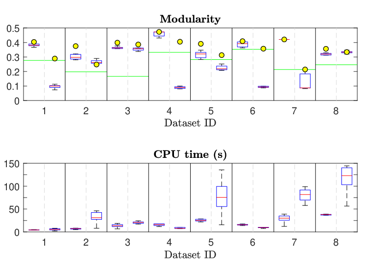
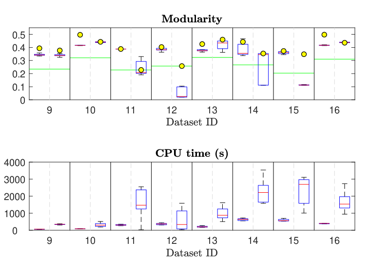


Table 3 shows mean and standard deviations of the modularity values obtained by FAST-ATVO and Generalized RatioDCA over 10 runs, each with a different randomly chosen starting point. This table confirms the behavior observed in Table 2: the average modularity value obtained with FAST-ATVO highly outperforms both the linear method and Generalized RatioDCA. Moreover, the modularity standard deviations shown in the table demonstrate that FAST-ATVO is generally more robust than Generalized RatioDCA.
| Dataset | Q | avg | std | avg | std | ||
|---|---|---|---|---|---|---|---|
| ID | Q | Q | Q | Q | |||
| 1 | 0.28 | 0.11 | 0.06 | 0.38 | 0.01 | 1.39 | 3.41 |
| 2 | 0.20 | 0.27 | 0.01 | 0.31 | 0.03 | 1.56 | 1.16 |
| 3 | 0.17 | 0.36 | 0.01 | 0.37 | 0.01 | 2.20 | 1.03 |
| 4 | 0.33 | 0.12 | 0.10 | 0.45 | 0.04 | 1.35 | 3.84 |
| 5 | 0.28 | 0.23 | 0.03 | 0.32 | 0.03 | 1.13 | 1.39 |
| 6 | 0.35 | 0.12 | 0.08 | 0.39 | 0.02 | 1.10 | 3.31 |
| 7 | 0.21 | 0.15 | 0.12 | 0.40 | 0.07 | 1.87 | 2.61 |
| 8 | 0.25 | 0.33 | 0.01 | 0.32 | 0.01 | 1.31 | 0.97 |
| 9 | 0.23 | 0.34 | 0.01 | 0.35 | 0.02 | 1.48 | 1.02 |
| 10 | 0.32 | 0.44 | 0.01 | 0.42 | 0.02 | 1.32 | 0.95 |
| 11 | 0.23 | 0.24 | 0.05 | 0.38 | 0.01 | 1.69 | 1.60 |
| 12 | 0.26 | 0.07 | 0.07 | 0.38 | 0.01 | 1.49 | 5.89 |
| 13 | 0.32 | 0.42 | 0.03 | 0.38 | 0.02 | 1.18 | 0.91 |
| 14 | 0.27 | 0.24 | 0.13 | 0.38 | 0.05 | 1.42 | 1.57 |
| 15 | 0.20 | 0.13 | 0.07 | 0.36 | 0.01 | 1.77 | 2.69 |
| 16 | 0.31 | 0.44 | 0.01 | 0.42 | 0.02 | 1.36 | 0.96 |
The results of Tables 2 and 3 are summarized and shown together in the boxplots of Figure 1 (removing outliers), where we also compare the execution times of the methods. The upper panels in Subfigures 1a and 1b show medians and quartiles of the modularity values obtained with FAST-ATVO (left columns) and Generalized RatioDCA (right columns) over 10 runs with random starting points, together with the value obtained using the linear eigenvector as a starting point (yellow dot). A straight green line shows, instead, the modularity value obtained with the linear spectral method. The lower panels in the subfigures show median and quartiles of execution times of FAST-ATVO and Generalized RatioDCA. As for the modularity values, we can see that FAST-ATVO is generally more efficient (as it requires a smaller median execution time) and more robust (as the variance of the CPU time is in general remarkably smaller).
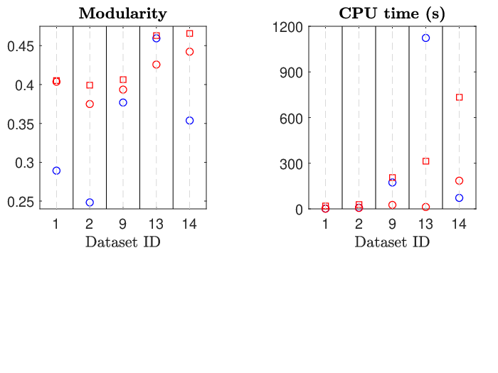
Finally, we report in Figure 3 the performance comparison among PS framework,
FAST-ATVO and Generalized RatioDCA.
For the three methods we use the linear eigenvector as starting point.
As we can easily see, the use of a global optimization strategy improves modularity values with respect to FAST-ATVO,
while guaranteeing good performances in terms of CPU time.
In particular, we notice that PS gives a modularity value higher than Generalized RatioDCA even for dataset Words28,
which was the only one where FAST-ATVO was outperformed by Generalized RatioDCA.
5 Conclusions
In this paper, we described a new modularity total variation approach for the leading community problem. We first proved that the original combinatorial problem is equivalent to the minimization of a suitably chosen continuous nonsmooth function (the modularity total variation) over a box. We then considered a smooth approximation of the continuous problem and developed an algorithmic framework to efficiently tackle it. The reported results show that the proposed method outperforms both Generalized RatioDCA and the linear method in terms of modularity value. Furthermore, the CPU time required to find those good solutions is usually significantly smaller than the CPU time needed to run Generalized RatioDCA. Hence, even if the modularity landscape is usually fraught with local optima (see, e.g., [29]), the proposed approach quickly finds solutions with good modularity values in the end. As far as we can see, the use of both the non-monotone line search and the randomized working set selection seems to be of help in avoiding/escaping “bad” local optima.
Future work might focus on adapting our strategy to efficiently handle applications where dense weighted graphs (such as similarity or correlation graphs) or multilayer graphs are required. Another interesting research direction might be analyzing how the described approach transfers and applies to other community detection techniques like, e.g., Belief Propagation [59], Stochastic Block Models [1] and Infomap [51].
Appendix A Detailed scheme and convergence analysis of FAST-ATVO
In this appendix, we report the detailed scheme of FAST-ATVO (a short scheme was given in Algorithm 1), together with its convergence analysis. The detailed scheme is reported below in Algorithm 4.
We see that every iteration starts with a non-stationary point . We first compute the active and non-active sets estimates as in step 2 and, if necessary, we evaluate the objective function (steps 3–9). More in detail, thanks to a non-monotone stabilization strategy, inspired from that used in [30], we can compute only once every iterations (if some tests described below are satisfied), rather than at each iteration, allowing us to save computational time. When we perform this function control, we compare with a reference value , which is the maximum among the last function evaluations: if we backtrack to the best point computed so far (i.e., ) and start a line search, otherwise we update and go on.
At steps 10–12, we choose a non-empty working set by a Gauss-Southwell-type (or greedy) rule: must contain the index of the variable that most violates stationarity. We then compute a search direction such that
| (17) |
with , and all the other components of are equal to zero. We see that, at each iteration, only a subset of variables (i.e., those in ) can be moved and the search direction is computed in the variable subspace defined by . The computation of the coefficient will be described in details later on.
Afterwards, in steps 13–21, if if sufficiently small we set and terminate the iteration. It means that, if that test is satisfied, we accept the unit stepsize without computing the objective function. Otherwise, we have two possibilities: if we backtrack to , else we update and go on. Both these cases are followed by a non-monotone line search.
In the last steps 22–23 of the algorithm, we compute the stepsize in order to set . We use a non-monotone Armijo line search with reference value equal to (which was first proposed in [30]).
Now, let us describe how we compute the search direction (step 12). As mentioned before, we choose a coefficient (in a finite positive interval) and compute as in (17), while all the other components of are set to zero. In this way, at each iteration we move only the variables in . In our experiments, we computed as a spectral (or Barzilai-Borwein) gradient direction (see, e.g., [26] and the references therein).
A.1 Global convergence proof
In order to prove the global convergence of FAST-ATVO we need some preliminary results that we derive below. Throughout the whole section, we use the notation of Algorithm 4.
First, we report a known result of non-monotone methods, whose proof can be easily adapted from the proof of Lemma 3 of [31] and is omitted here for the sake of brevity.
Lemma 4.
Assume that is an infinite sequence of points produced by FAST-ATVO. Then,
| (18) | |||
| (19) |
Further, we state the following technical lemma
Lemma 5.
There exist subsequences , , and sets , , , such that
with and .
Proof.
The thesis is an immediate consequence of the fact that , , , are subsets of a finite set of indices and the sequences , , are bounded. In particular, the latter property itself follows from the fact that , from the compactness of the feasible set and from the compactness of the feasible set combined with the definition of and the continuity of , respectively. ∎
Using the previous lemmas, we derive the following result.
Lemma 6.
Assume that is an infinite sequence of points produced by FAST-ATVO. Then,
Proof.
We proceed by contradiction and we assume that the result is not true. Let , , and , , , be as in Lemma 5. Using (19) and the continuity of the projection operator, we can thus write
| (20) |
In the sequel, we show that the above limit leads to , getting a contradiction. To this extent, let us first observe that, from the definition of and the continuity of , we have
| (21) |
for some . Moreover, from our estimates (10) and the continuity of , there exists an iteration such that
| (22a) | |||
| (22b) | |||
Now, let us consider any index . We can distinguish four possible cases.
- (i)
. From the definition of the search direction, it follows that .
- (ii)
such that . From (20) and the fact that , we obtain .
- (iii)
- (iv)
such that . Reasoning as above, we get .
We thus obtain , leading to a contradiction. ∎
We can now show that the sequence of directional derivatives converges to zero, which will be crucial to prove the global convergence of the algorithm.
Proposition 2.
Assume that is an infinite sequence of points produced by FAST-ATVO. Then,
| (23) |
Proof.
By contradiction, we assume that (23) does not hold. There must exist , , and , , , defined as in Lemma 5, which also satisfy
| (24) |
Combining (24) with Lemma 6, we obtain
| (25) |
Therefore, there exist two further infinite subsequences, that, with a slight abuse of notation, we still denote by and , such that for all . From Algorithm 4, can be less than if and only if it is computed by the non-monotone Armijo line search using (see steps 22–23). It follows that
| (26) |
where . Let us write the point as follows:
| (27) |
where
| (28) |
or equivalently,
Using (25), the feasibility of points and the fact that is bounded, we have
| (29) |
Now, from (26) and (27) we can write
| (30) |
By the mean value theorem, we also have
| (31) |
where and . Using (25), (29) and the fact that is bounded, we obtain
| (32) |
Moreover, from (30) and (31), we have
| (33) |
In the following, we show that
| (34) |
From (28) and the fact that each is feasible, we first observe that
| (35) |
Now, we consider any index and we analyze four possible cases, in order to show that (34) holds.
- (i)
. From the rule used to compute , we have . Using (35) it follows that for all , implying that
(36) - (ii)
- (iii)
such that . Since and is continuous, from our estimates (10) (and recalling that ) we have
(38) Now, we also show that there exists such that
(39) Indeed, since , for all sufficiently large we have for some . Using (25) and the fact that is bounded, for all sufficiently large we have
which, combined with (28), implies (39). Let us partition into and , such that every belongs to if and only if (and then, every belongs to if and only if ). Assuming without loss of generality that both and are infinite, we now analyze the corresponding subsequences.
- (iv)
such that . Reasoning as in the previous case, we obtain
(44)
Therefore, (34) follows from (36), (37), (43) and (44). Combining (34) with (33), we can write
where the last two equalities follow from the continuity of and the fact that both and converge to . Using (24), we finally obtain , with and , which leads to a contradiction. ∎
We are finally ready to prove the global convergence of FAST-ATVO to stationary points.
Proof of Theorem 2.
Assume that the sequence generated by FAST-ATVO is infinite and let be a limit point of . Further, let , , and , , , be as in Lemma 5. Using the stationarity conditions (9), we can measure the stationarity violation of any feasible point by the following functions:
Namely, a feasible point is stationary if and only if for all . Now, arguing by contradiction, assume that is non-stationary. Then, an index such that exists. Note that it must hold that
| (45) |
Moreover, from the continuity of , there exist and such that
| (46) |
Now, we consider four possible cases.
- (i)
- (ii)
. From (10b) we have and for all . Then, we obtain a contradiction by the same arguments used above.
- (iii)
- (iv)
. Without loss of generality, we can assume that the index computed at step 10 is constant and equal to for all (passing into a subsequence if necessary). So, using the definition of , for all we can write
Since does not violate stationarity (from the fact that , as analyzed above), the continuity of the projection operator and the continuity of imply that
We hence have , which gives a contradiction.
Therefore must be a stationary point. ∎
References
- Abbe [2017] E. Abbe. Community detection and stochastic block models: recent developments. The Journal of Machine Learning Research, 18(1):6446–6531, 2017.
- Andreani et al. [2010] R. Andreani, E. G. Birgin, J. M. Martínez, and M. L. Schuverdt. Second-order negative-curvature methods for box-constrained and general constrained optimization. Comput. Optim. Appl., 45(2):209–236, 2010.
- Bach [2013] F. Bach. Learning with submodular functions: A convex optimization perspective. Foundations and Trends in Machine Learning, 6(2-3):145–373, 2013. ISSN 1935-8237.
- Batagelj and Mrvar [2006] V. Batagelj and A. Mrvar. Pajek datasets collection, 2006. URL http://vlado.fmf.uni-lj.si/pub/networks/data/.
- Beck and Teboulle [2009] A. Beck and M. Teboulle. A fast iterative shrinkage-thresholding algorithm for linear inverse problems. SIAM J. Imaging Sci., 2:183–202, 2009.
- Birgin and Martínez [2002] E. G. Birgin and J. M. Martínez. Large-scale active-set box-constrained optimization method with spectral projected gradients. Comput. Optim. Appl., 23(1):101–125, 2002.
- Blondel et al. [2008] V. D. Blondel, J.-L. Guillaume, R. Lambiotte, and E. Lefebvre. Fast unfolding of communities in large networks. J. Stat. Mech. Theory Exp., 2008:P10008, 2008.
- Boyd et al. [2018] Z. M. Boyd, E. Bae, X.-C. Tai, and A. L. Bertozzi. Simplified energy landscape for modularity using total variation. SIAM J. Appl. Math., 78(5):2439–2464, 2018.
- Brandes et al. [2007] U. Brandes, D. Delling, M. Gaertler, R. Görke, M. Hoefer, Z. Nikoloski, and D. Wagner. On finding graph clusterings with maximum modularity. In International Workshop on Graph-Theoretic Concepts in Computer Science, pages 121–132. Springer, 2007.
- Bresson et al. [2013] X. Bresson, T. Laurent, D. Uminsky, and J. Von Brecht. Multiclass total variation clustering. In Adv. Neural Inf. Process. Syst. (NIPS), pages 1421–1429, 2013.
- Bühler and Hein [2009] T. Bühler and M. Hein. Spectral clustering based on the graph -Laplacian. In Proceedings of the 26th Annual International Conference on Machine Learning (ICML), pages 81–88, 2009.
- Chambolle and Pock [2011] A. Chambolle and T. Pock. A first-order primal-dual algorithm for convex problems with applications to imaging. J. Math. Imaging Vision, 40:120–145, 2011.
- Cho et al. [2011] E. Cho, S. A. Myers, and J. Leskovec. Friendship and mobility: User movement in location-based social networks. In ACM SIGKDD International Conference on Knowledge Discovery and Data Mining (KDD), 2011.
- Chung and Lu [2006] F. R. K. Chung and L. Lu. Complex graphs and networks, volume 107. American Mathematical Society, Providence, 2006.
- Cinelli et al. [2019] M. Cinelli, L. Peel, A. Iovanella, and J.-C. Delvenne. Network constraints on the mixing patterns of binary node metadata. arXiv preprint arXiv:1908.04588, 2019.
- Clauset et al. [2004] A. Clauset, M. E. J. Newman, and C. Moore. Finding community structure in very large networks. Phys. Rev. E, 70:066111, 2004.
- Cristofari et al. [2017] A. Cristofari, M. De Santis, S. Lucidi, and F. Rinaldi. A two-stage active-set algorithm for bound-constrained optimization. J. Optim. Theory Appl., 172(2):369–401, 2017.
- Curtis et al. [2015] F. E. Curtis, Z. Han, and D. P. Robinson. A globally convergent primal-dual active-set framework for large-scale convex quadratic optimization. Comput. Optim. Appl., 60(2):311–341, 2015.
- De Santis et al. [2012] M. De Santis, G. Di Pillo, and S. Lucidi. An active set feasible method for large-scale minimization problems with bound constraints. Comput. Optim. Appl., 53(2):395–423, 2012.
- Di Pillo and Grippo [1984] G. Di Pillo and L. Grippo. A class of continuously differentiable exact penalty function algorithms for nonlinear programming problems. In System Modelling and Optimization, pages 246–256. Springer, 1984.
- Duch and Arenas [2005] J. Duch and A. Arenas. Community detection in complex networks using extremal optimization. Phys. Rev. E, 72:027104, 2005.
- Facchinei and Lucidi [1995] F. Facchinei and S. Lucidi. Quadratically and superlinearly convergent algorithms for the solution of inequality constrained minimization problems. J. Optim. Theory Appl., 85(2):265–289, 1995.
- Fasino and Tudisco [2014] D. Fasino and F. Tudisco. An algebraic analysis of the graph modularity. SIAM J. Matrix Anal. Appl, 35:997–1018, 2014.
- Fasino and Tudisco [2016] D. Fasino and F. Tudisco. Generalized modularity matrices. Linear Algebra Appl., 502:327–345, 2016.
- Ferreau et al. [2014] H. J. Ferreau, C. Kirches, A. Potschka, H. G. Bock, and M. Diehl. qpoases: A parametric active-set algorithm for quadratic programming. Math. Program. Comput., 6(4):327–363, 2014.
- Fletcher [2005] R. Fletcher. On the Barzilai-Borwein method. In Optimization and control with applications, pages 235–256. Springer, 2005.
- Fortunato [2010] S. Fortunato. Community detection in graphs. Phys. Rep., 486:75–174, 2010.
- Fortunato and Hric [2016] S. Fortunato and D. Hric. Community detection in networks: A user guide. Phys. Rep., 659:1–44, 2016.
- Good et al. [2010] B. H. Good, Y.-A. de Montjoye, and A. Clauset. Performance of modularity maximization in practical contexts. Phys. Rev. E, 81(4):046106, 2010.
- Grippo et al. [1986] L. Grippo, F. Lampariello, and S. Lucidi. A nonmonotone line search technique for newton’s method. SIAM J. Numer. Anal., 23(4):707–716, 1986.
- Grippo et al. [1991] L. Grippo, F. Lampariello, and S. Lucidi. A class of nonmonotone stabilization methods in unconstrained optimization. Numer. Math., 59(1):779–805, 1991.
- Grosso et al. [2007] A. Grosso, M. Locatelli, and F. Schoen. A population-based approach for hard global optimization problems based on dissimilarity measures. Math. Program., 110(2):373–404, 2007.
- Guimera et al. [2004] R. Guimera, M. Sales-Pardo, and L. A. N. Amaral. Modularity from fluctuations in random graphs and complex networks. Phys. Rev. E, 70:025101, 2004.
- Hager and Zhang [2006] W. W. Hager and H. Zhang. A new active set algorithm for box constrained optimization. SIAM J. Optim., 17(2):526–557, 2006.
- Hartwell et al. [1999] L. H. Hartwell, J. J. Hopfield, S. Leibler, and A. W. Murray. From molecular to modular cell biology. Nature, 402(6761supp):C47, 1999.
- Hein and Bühler [2010] M. Hein and T. Bühler. An inverse power method for nonlinear eigenproblems with applications in 1-spectral clustering and sparse PCA. In Adv. Neural Inf. Process. Syst. 23 (NIPS), pages 847–855, 2010.
- Hein and Setzer [2011] M. Hein and S. Setzer. Beyond spectral clustering-tight relaxations of balanced graph cuts. In Adv. Neural Inf. Process. Syst. (NIPS), pages 2366–2374, 2011.
- Hu et al. [2013] H. Hu, T. Laurent, M. A. Porter, and A. L. Bertozzi. A method based on total variation for network modularity optimization using the MBO scheme. SIAM J. Appl. Math., 73:2224–2246, 2013.
- Lancichinetti and Fortunato [2009] A. Lancichinetti and S. Fortunato. Community detection algorithms: a comparative analysis. Phys. Rev. E, 80:056117, 2009.
- Leary [2000] R. H. Leary. Global optimization on funneling landscapes. J. Global Optim., 18(4):367–383, 2000.
- Leskovec et al. [2005] J. Leskovec, J. Kleinberg, and C. Faloutsos. Graphs over time: Densification laws, shrinking diameters and possible explanations. In SIGKDD International Conference on Knowledge Discovery and Data Mining (KDD), 2005.
- Leskovec et al. [2007] J. Leskovec, J. Kleinberg, and C. Faloutsos. Graph evolution: Densification and shrinking diameters. In ACM Trans. Knowledge Discovery from Data, 2007.
- Mercado et al. [2016] P. Mercado, F. Tudisco, and M. Hein. Clustering signed networks with the geometric mean of Laplacians. In Adv. Neural Inf. Process. Syst.(NIPS), 2016.
- Mercado et al. [2018] P. Mercado, A. Gautier, F. Tudisco, and M. Hein. The power mean Laplacian for multilayer graph clustering. In Proceedings of the 21st International Conference on Artificial Intelligence and Statistics (AISTATS), volume 84 of Proceedings of Machine Learning Research, pages 1828–1838, 2018.
- Newman [2006] M. E. J. Newman. Finding community structure in networks using the eigenvectors of matrices. Phys. Rev. E, 74:036104, 2006.
- Newman [2010] M. E. J. Newman. Networks: an introduction. Oxford University Press, 2010.
- Newman and Girvan [2004] M. E. J. Newman and M. Girvan. Finding and evaluating community structure in networks. Phys. Rev. E, 69:026113, 2004.
- Nocedal and Wright [2006] J. Nocedal and S. J. Wright. Sequential quadratic programming. Springer, 2006.
- Ozer et al. [2016] M. Ozer, N. Kim, and H. Davulcu. Community detection in political twitter networks using nonnegative matrix factorization methods. In Proceedings of the 2016 IEEE/ACM International Conference on Advances in Social Networks Analysis and Mining, pages 81–88. IEEE Press, 2016.
- Porter et al. [2009] M. A. Porter, J.-P. Onnela, and P. J. Mucha. Communities in networks. Notices Amer. Math. Soc., 56:1082–1097, 2009.
- Rosvall et al. [2009] M. Rosvall, D. Axelsson, and C. T. Bergstrom. The map equation. The European Physical Journal Special Topics, 178(1):13–23, 2009.
- Safro et al. [2015] I. Safro, P. Sanders, and C. Schulz. Advanced coarsening schemes for graph partitioning. Journal of Experimental Algorithmics (JEA), 19:1–24, 2015.
- Schaeffer [2007] S. E. Schaeffer. Graph clustering. Comput. Sci. Rev., 1:27–64, 2007.
- Shen and Cheng [2010] H.-W. Shen and X.-Q. Cheng. Spectral methods for the detection of network community structure: a comparative analysis. J. Stat. Mech. Theory Exp., 2010:P10020, 2010.
- Traag et al. [2011] V. A. Traag, P. Van Dooren, and Y. Nesterov. Narrow scope for resolution-limit-free community detection. Phys. Rev. E, 84:016114, 2011.
- Tudisco and Hein [2018] F. Tudisco and M. Hein. A nodal domain theorem and a higher-order Cheeger inequality for the graph -Laplacian. J. Spectr. Theory, 8:883–908, 2018.
- Tudisco and Higham [in press] F. Tudisco and D. J. Higham. A nonlinear spectral method for core-periphery detection in networks. SIAM J. Mathematics of Data Science, in press.
- Tudisco et al. [2018] F. Tudisco, P. Mercado, and M. Hein. Community detection in networks via nonlinear modularity eigenvectors. SIAM J. Appl. Math., 78:2393–2419, 2018.
- Zhang and Moore [2014] P. Zhang and C. Moore. Scalable detection of statistically significant communities and hierarchies, using message passing for modularity. Proceedings of the National Academy of Sciences, 111(51):18144–18149, 2014.