A Sequential Composition Framework for Coordinating Multi-Robot Behaviors
Abstract
A number of coordinated behaviors have been proposed for achieving specific tasks for multi-robot systems. However, since most applications require more than one such behavior, one needs to be able to compose together sequences of behaviors while respecting local information flow constraints. Specifically, when the inter-agent communication depends on inter-robot distances, these constraints translate into particular configurations that must be reached in finite time in order for the system to be able to transition between the behaviors. To this end, we develop a distributed framework based on finite-time convergence control barrier functions that enables a team of robots to adjust its configuration in order to meet the communication requirements for the different tasks. In order to demonstrate the significance of the proposed framework, we implemented a full-scale scenario where a team of eight planar robots explore an urban environment in order to localize and rescue a subject.
Index Terms:
Multi-Robot Systems, Networked Robots, Control Barrier Functions, Behavior-Based SystemsI Introduction
As our understanding of how to structure control and coordination protocols for teams of robots increases, a number of application domains have been identified, such as entertainment [1][2], surveillance [3] [4], manipulation [5], and search-and-rescue [6]. Along with a decrease in the production and manufacturing costs associated with the platforms themselves, these applications have been enabled by a number of theoretical results that have emerged at the intersection of different disciplines such as robotics, controls, computer science, and graph theory [7].
From a motion controls perspective, one notable requirement is given by the need to define actions capable to solve team-wise objectives on the basis of locally available information. For instance, different extensions of the consensus equation have been used to arrive at locally defined controllers with provable, global convergence properties [8]. In this way, it is possible to construct coordinated controllers for the solution of motion control problems, such as rendezvous [9] [10], cyclic pursuit [11], formation control [12] [13], coverage [14] [3], leader-based control [15], and flocking [16]. Particular instantiations of some of these behaviors are shown in Fig. 1 on a group of six simulated differential drive robots.


For the correct execution of the controllers mentioned, a sufficiently rich set of information needs to be available to the robots. Representing the flow of information between the robots through graphs, with vertices and edges being respectively the robots and the pair-wise ability of sharing information, those conditions can be encoded in terms of particular graphs that need to exist between the robots. For example, rendezvous requires a spanning out-branching tree [15], cyclic-pursuit requires a cyclic graph [11], formation control a rigid graph [15], and a Delaunay graph is required for most of coverage control problems [14].
Even though the coordinated behaviors mentioned above can address a number of different tasks, they have limited utility in the context of real-world missions, which can rarely be represented as single tasks. However, the utility of these behaviors can be greatly expanded if they are sequenced together, which is the primary consideration in this paper. But, for a construction like this to work, it is necessary that the required information is available to the robots as they transition from one behavior to the next.
As such, the problem of composing different behaviors, can be recast in terms of the ability of the robots to establish the interactions needed at each stage of a mission. In particular, when the communication between agents depends on their relative configurations (e.g. relative distance or orientation), realizing a certain communication structure directly affects the configuration of the system, which in turn, affects the execution of the mission itself. In order to overcome this coupling, we separate the problem of generating a sequence of behaviors that corresponds to the solution of a mission objective (e.g. [17]) from their composition. In this work we focus on the problem of designing a composition framework given a sequence of coordinated behaviors. Although the focus of this paper is confined to motion control tasks, our framework is applicable to other forms of autonomous collaboration where desired interaction structures between the robots are required by the mission, e.g., sharing of resources in heterogeneous teams [18] or coordinated manipulation [19].
The contribution of this paper is twofold. Firstly, extending the results in [20], we propose a fully decentralized framework for composing a given sequence of multi-robot coordinated behaviors. Secondly, responding to the lack of established large-scale scenarios for the testing of multi-robot techniques, we propose a scenario called Securing a Building, which is rich and complex enough to capture many challenges and objectives of real-world implementations. The significance of our framework is demonstrated through implementation of the Securing a Building scenario on a team of mobile robots.
The remaining of this paper is organized as follows. In Section III we review the definition of finite-time convergence barrier functions, while in Section IV we present a centralized multi-robot composition framework, which is extended to a fully decentralized formulation in Section VI. In Section VII, we describe the Securing a Building case study and its implementation. Finally, motivated by the lack of well-established scenarios for testing and comparing multi-agent robotics techniques, in Appendix A we discuss supportive arguments for considering the Securing a Building as a multi-robot benchmark scenario.
II Related Work
The problem of partitioning complex objectives into simpler tasks can be solved by sequentially composing primitives, e.g., [21], or by blending them simultaneously in a hierarchical fashion. An example of hierarchical composition for single robot motion control is navigation between points while avoiding obstacles, e.g., [22]. In general, the problem of controlling a system by composing different modes of operation pertains to hybrid systems and multi-modal control domains [23].
Because of the complexity emerging from the composition of distinct controllers, guarantees on the safety and correctness of the final results need to be established [24]. Provable correct composition of control policies is investigated in the formal methods literature. Recently, compositional strategies inspired from formal methods have been used for the development of control strategies for multi-robot systems [25, 26, 27, 28]. In particular, the authors of [25] use tools from linear temporal logic (LTL) for the specification of behaviors to be executed by the system. The solution is based on a sequence of constrained reachability problems, each consisting of a target set to be reached in finite time and a safety set within which the system must stay at all times. A related approach is developed in [26], where the problem of prescribed-time convergence to spatio-temporal specifications is formulated using control barrier functions. The authors in [27] discuss a hierarchical decomposition method for controller synthesis given LTL specifications.
In the context of controllers composition for multi-robot systems, in [29] the authors use symbolic methods in order to generate high-level instructions from form of human-like language. The authors of [30] introduce a framework for the composition of controllers in robotic systems using Petri Nets. In [31], behaviors from the Null-Space-Behaviors framework are combined in order to solve ad-hoc tasks, such as perimeter patrol. A supervisor, represented as a finite state automata, selects high-level behaviors by assembling low-level behaviors. In [17], a revised version of the algorithm is used to generate an optimal path of behaviors, such that the overall cost of the mission is minimized. Similarly, in [32] motion planning for a team of quadcopters is solved by defining higher level motion primitives obtained by a spatial partition of the environment. However, none of these approaches specifically address the problem of correct composition between primitives, which is the focus of this paper.
As discussed in the previous section, coordination between agents is possible only if particular interactions exist between the robots. In multi-robot systems, interaction requirements are commonly investigated in terms of connectivity maintenance, i.e., a certain graph or node-connectivity needs to be guaranteed at all times. Methods employed in the solution to this problem include edge weight functions [33], control rules based on estimate of algebraic connectivity [34], hybrid control [35], passivity [36], and barrier functions [37]. If connectivity between agents needs to be guaranteed in non-nominal circumstances, resilient solutions must be in place as well, e.g., [18], [38], and [39]. Notably, a technique based on graph process specifications for the sequential composition of different multi-agent controllers is discussed in [40]. Similar to our work, the authors in [40] bridge the gap between composition of controllers and the topology requirements by encoding requisites for each controller in terms of graphs. However, while in [40] incompatible controllers are combined through the introduction of a bridging controller, in our approach controllers are minimally modified by the robots in order to satisfy upcoming requirements. Our approach significantly reduces the complexity of the composition process, minimizes the energy spent by the robots to switch between behaviors, and can accommodate additional constraints, such as inter-robot collisions and obstacles avoidance.
III Finite-Time Barrier Functions
In this section we review the general definition of Finite-time Convergence Control Barrier Function (FCBF) which was first introduced in [20] and inspired by the finite-time stability analysis for autonomous system introduced in [41]. Given a dynamical system operating in an open set and a set , barrier functions [42] are Lyapunov-like functions that guarantee forward invariance of with respect to the state of the system. In other words, if an appropriate barrier function exists, it can be used to show that if the state of a system is in at some time, it will be in thereafter. The concept of barrier functions was extended to Zeroing Control Barrier Functions (ZCBF) in [42], where asymptotic convergence of the state to the set was discussed. Thus, provided that an appropriate ZCBF exists, if the state of the system is not in at some initial time, it will asymptotically converge to .
As discussed in the introduction, before execution of a coordinated behavior, robots need to satisfy certain spatial configurations imposed by the behavior itself. Importantly asymptotic convergence to the correct configuration is not sufficient. In fact, if we consider as the joint set of all initial configurations required for a particular behavior, the state must strictly belong to for the behavior to work properly. Following this observation, the need for a finite-time convergence extension of the previous concepts becomes clear. In particular, denoting the state of the system as , we are interested in verifying the following conditions:
- •
if , then for all
- •
if , then for some .
In order to do this, we encode the set , through the superzero-level set of a continuously differentiable function , i.e.,
| (1) |
Definition III.1
We introduce the following class- function
| (2) |
with and , which is continuous everywhere and locally Lipschitz everywhere except at the origin [41].
Definition III.2
Following from the definition above, we define the set of admissible control inputs as
| (5) |
Theorem III.3
In conclusion, by selecting a controller that verifies condition (6), both forward invariance and finite-time convergence to the desired set are guaranteed.
IV Problem Formulation
We denote the state of a team of homogeneous mobile robots operating in a -dimensional and connected domain as where is the position of robot at time . As part of the coordinated nature of the behaviors being performed by the robots, each robot executes a control protocol which depends on the state of the subset of robots with which it interacts. We assume robots can communicate if the distance between them is less or equal to a sensing threshold . Thus, the list of possible interactions between agents are described by a time-varying, undirected, proximity graph , where is the set of nodes representing the robots and is the set of interacting pairs at time , where
| (8) |
For each robot , we denote the set of available neighbors at time as , which depends on the position of the robots at time .
The ensemble dynamics of the multi-agent system is described by
| (9) |
where and are continuous locally Lipschitz continuous functions and is the vector of inputs, which depends on the particular behavior being executed. At all times, the control input in (9) is given by a controller , which can be defined as a state feedback law or by a combination of both external parameters and state feedback law , where is a space of parameters appropriate for the behavior. For instance, the controller corresponding to a weighted consensus belongs to the first case. On the other side, a leader-follower protocol where followers maintain prescribed inter-agent distances is described by a controller that depends on both state feedback (followers’ control) and exogenous parameters (leader’s goal) (see Section VI for examples).
We represent a mission by an ordered sequence of coordinated behaviors
| (10) |
The behavior in is defined by the pair
| (11) |
where represents the coordinated controller described above and is the interaction graph required by behavior to function properly. We assume the list of behaviors to be fixed and available to all robots. We will use the term behavior to refer to a generalized multi-robot controller in the form (11) and to task as the objective of the controller.
As discussed in Section I, each behavior requires a certain interaction structure between the robots (i.e., pairs of robots that need to be neighbors). With reference to (11), we describe an interaction structure via the graph . Thus, denoting by and the starting and ending times for behavior , the robots’ configuration needs to satisfy for all . In other words, as shown in Fig. 2, the interaction structure required by each behavior needs to be a spanning graph of the graph induced by the state of the agents during the interval of time the behavior is executed. At this point, given a list of behaviors constituting the mission and the corresponding multi-robot controllers, we want to design a procedure that enables robots to assemble and maintain the communication graph required by each behavior.
Problem IV.1
Given an ordered sequence of coordinated behaviors , where each can be completed by the robots in finite-time, design a feedback control policy to compose the behaviors such that
| (12) |
V Composition of Coordinated Behaviors
In addition to the list , transitions between behaviors need to be synchronized, i.e., for each behavior , , robots must 1) start assembling only after all robots have completed and 2) start executing only after condition is satisfied. We assume the existence of a discrete counter which indicates the active behavior and a binary signal
| (13) |
which describes whether the interaction structure required by behavior is available. In this section, we assume both signals to be controlled by a supervisor and made available to the robots at all times, e.g., through a dedicated static communication network. In the next section, we discuss the extension to a fully distributed framework.
Following from the communication modality assumed for the robots, communication constraints can be expressed in terms of relative distance between the robots. In other words, behavior can be correctly executed if, for all , all the distances between pairs in are below the proximity threshold . To this end, a convenient pair-wise connectivity FCBF can be defined as
| (14) |
and we note that if , then . In addition, the edge-level and ensemble-level connectivity constraint sets for behavior are
| (15) | ||||
| (16) |
Following the definition given in (5), the admissible set of control inputs that guarantees finite-time convergence to is:
| (17) |
Theorem V.1
Denoting with the initial state of the system with dynamics (9), any controller such that for all , will drive the system to within time
| (18) |
Proof:
Consider all pairs of agents and , such that . If , i.e., agents and are within communication distance, the forward invariance property of , guarantees that and will stay connected. In this case, the state will reach , within time . On the other side, consider . Any satisfies the finite-time convergence barrier certificates, and because of Theorem III.3, if , then , with
| (19) |
Since every communication constraint will be reached within time , the total time required to drive to is upper bounded by
| (20) |
∎When selecting control inputs from set (17), the system (9) will satisfy requirements for behavior in finite time.
V-A Finite-Time Convergence Control Barrier Functions
Once behavior is completed, robots are required to converge to the set before behavior can start. Under the lead of the external supervisor, the change of behavior is communicated to the robots through the signal , which transitions from to once is completed. Now, although finite-time convergence to can be achieved by selecting any control input in , we seek to minimally perturb the execution of the behavior just concluded, namely . This can be accomplished by solving a problem similar to the one proposed in [43], which we adapt to our framework. Denoting with the nominal control input from behavior , during transition between and the actual control input to the robots is defined as
| (21) |
subject to
| (22) |
for all . Once all required edges are established (i.e., ), edges in are no longer necessary. At this point, under the effect of the controller , the list of constraints in (22) is substituted with
| (23) |
for all . Since the cost function is convex and the inequality constraints (22) and (23) are control affine, the problem can be solved in real-time. In conclusion, because of the finite-time convergence and forward invariance properties of the above formulation, if can be completed and a solution to (21-22) (or (21-23)) exists, robots will converge to the configuration required by , and maintain it throughout its execution.
Remark V.1
The solution of (21-22) (or (21-23)) is contingent upon the existence of a control input capable to solve all constraints. In other words, (or ) should not be empty for all times. For this, it is necessary that a robot’s configuration that satisfies all constraints of the problem exists. However, this is not sufficient as the progress towards the desired configuration might be obstructed by constraints on the actuators or deadlock configurations. Although we do not address this directly, it is possible to mitigate feasibility issues by considering, for example, constraints relaxation, sum of squares barrier functions, or pre-defined back-up controllers (see [44] and references therein).
V-B Initial Constraints
In addition to the communication constraints considered above, certain missions might require additional conditions to be met before each behavior can start. For example, during the exploration tasks it might be desirable for one robot to always stay within range of communication with a human-operator, or to maintain a minimum distance from an unsafe area. Assuming requires a number of distinct of such constraints, we encode the entire set of initial conditions through a list of barrier functions , with :
| (24) |
Following this definition, we define a set of admissible control inputs similar to the one in (17) that will drive the state of the system to the desired set within finite time:
| (25) |
VI Distributed Composition of Behaviors
The composition framework discussed in the previous section reduces to the team-wise minimum norm controller (21), which is not directly solvable by individual robots. In addition to this, a centralized supervisor is needed in order to synchronize behavior transitions. In this section, we formulate a decentralized solution to problem IV.1 which can be implemented by the robots using only information from their neighbors. Furthermore, we also include those additional constraints necessary for the safe operations of the robots, e.g., inter-agent collisions and obstacles avoidance [37]. The formulation is derived following the approach described in [45], which we adapt here to our framework.
VI-A Distributed Finite-Time Convergence Control Barrier Functions
The limitation in solving problem (21) in a distributed fashion is represented by the fact that knowledge of dynamics, input , and state for the entire team need to be available. In addition, solution of (21), provides the control inputs for the entire team, which are unnecessary to the individual robots.
In order to develop the correct decentralized formulation of (21), we first define a decomposition of the dynamics (9). We denote by and configuration space and set of feasible controls for agent respectively. In addition, by denoting with the node-level terms of the control affine dynamics of agent , the ensemble dynamics can be written as:
| (27) |
where is the robot’s control input, is the Kronecker product, and and are vector of ones and identity matrix of size respectively.
Let’s consider two sequential behaviors and . Upon completion of , for all edges , robots’ configuration should satisfy
| (28) |
From the robot’s point of view, the set of constraints that need to be satisfied in order to execute the new behavior are
| (29) |
where we recall that is the set of neighbors to robot required by behavior . However, since constraint (29) appears exactly twice across the team of robots, it can be relaxed by considering the admissible set of control inputs
| (30) |
with
| (31) |
where dependence from and is omitted for clarity.
Theorem VI.1
Denoting with the initial state of a multi-agent system with dynamics described as in (27), any controller such that for all , will drive the ensemble state to within time
| (32) |
Proof:
From Theorem III.3, agents and , with , will satisfy in finite time if
| (33) |
| (34) | ||||
which will be satisfied if both agents and satisfy the constraint
| (35) |
In addition, as discussed in Theorem V.1, constraint (34) will still be satisfied at time
| (36) |
The same argument can be repeated for all pairs , and condition will be satisfied within time
| (37) |
∎
Applying the same design principle described in Section V-A, the minimally invasive control action can be computed by each robot as
| (38) |
subject to
| (39) |
Similarly to constraint (22), once all edges in are available, constraint (39) is substituted with
| (40) |
which remains active until is completed.
We note that, in order for agent to respect (40), the only external information needed is the state of all current neighbors, i.e. for all . On the other side, in order to respect (39), robots need to have access to the state of the future neighbors. This requirement can be satisfied through a state estimation scheme (e.g. EKF [46]), which in turn requires knowledge of robots’ dynamics (known for homogeneous teams) or network localization techniques [47].
Remark VI.1
The ability of each robot to have access to an estimate of their future neighbors’ state does not eliminate the necessity of establishing neighborhood relationships. In fact, a certain proximity structure between robots might be required by desired controllers’ performance that cannot be met through state estimations, or by collaboration tasks that require physical interaction between the robots, e.g. collaborative manipulation [19], sharing of resources [18].
VI-B Additional Constraints
In addition to the proximity constraints discussed above, additional limitations might be imposed on the robots’ configuration by the mission and the environment. For illustrative purposes, we consider inter-robots collisions and obstacle avoidance. Following the approach described in [37], we encode each pair-wise separation condition through the following barrier certificate
| (41) |
and the minimum separation between the robots is satisfied if , for all physical neighbors .
Similarly, avoidance of fixed obstacles can be introduce by considering ellipsoidal regions of the domain, described by centers . For every agent-obstacle pair we define a pairwise barrier function as
| (42) | ||||
| (43) |
The object avoidance constraints are satisfied if , for all and .
Collecting all the constraints, we expand the problem formulation in (21) to
VI-C Decentralized Behaviors Sequencing
For the correct execution of the behaviors sequencing, each robot should start assembling a new graph only after all other robots have completed the current behavior. Similarly, a new behavior should start once all robots satisfy the neighbors’ requirements for it. Now, we describe a decentralized strategy that allows execution of these two transitions without the need of a supervisor, nor synchronization between the robots.
With reference to Fig. 3, at any given time, each robot’s mode of operation is described by a binary variable that describes whether robot is assembling the graph for an upcoming behavior () or executing a behavior (). Without loss of generality, assume robots’ initial configuration satisfies the communication requirements for the first behavior, which is then executed (). Once all robots have completed the first behavior, they start assembling the graph required by the following one (), while minimally perturbing the behavior just concluded. Once the new graph is satisfied , robots start behavior and exit from assembly mode (). This process repeats, until no successive behavior exists.
A correct execution of this process requires robot to agree on when to perform transitions and . To this end, we take inspiration from the consensus-based algorithm described in [48] and we note that this choice is not central to the contribution of this paper. For each robot, we define a binary variable available only to robot , that denotes whether robot itself has completed its current task ( if robot has not completed its current task). In addition, we introduce a variable , shared among neighbors, continuously updated through the following consensus-based process
| (45) |
where represent the variable’s value after the update. Owing to the diffusion of throughout the network, we can interpret ’s as local measures of the team-wise completion of a task. As proved in [48], if for all (i.e., all robots are capable to complete the current behavior), by following (45), , for all . Therefore, robot starts assembling a new communication graph once the value of is close enough to (see [48] for a discussion on how to choose the switching threshold). A similar process is used for the transition , where we replace and with and respectively. The distributed sequencing procedure is summarized in Algorithm 1.
for do
;
VI-D Applications


We implemented the distributed sequencing framework on the Robotarium [49], on a team of differential drive robots. For this example, controllers are designed assuming a single integrator model, i.e. and . In this example, robots execute a transition between two behaviors, where is a cyclic-pursuit behavior and is a formation assembly with leader. Cyclic-pursuit behavior is obtained through the following controller:
where is the rotation matrix of angle , which is related to the desired cycle radius. Importantly, for this behavior to work, the communication graph must be a cycle graph. Considering robot as leader, the formation control behavior can be achieved with
where is the desired inter-robot distance, is the leader’s goal, and the corresponding proportional gain. In the case of formation control, it is known that the Euclidean embedding of must be a rigid framework (see for instance [15] and references therein). With reference to Fig. 4, robots initially execute for a certain amount of time (a). Once completed (b) (green patches represent robots that have completed their current behavior), robots start assembling (c), after which is executed until is below a pre-defined threshold (d-f).
In Fig. 5 we can observe the value of the two consensus variables and for all robots during the behavior transition. Background colors represent the time intervals during which the two behaviors were executed, while the darker region in the middle corresponds to the assembly of the new graph. We observe the assembly and task variables and approaching the value simultaneously for all robots, thus triggering a synchronized start of the successive phase.
The robustness of our technique was tested by simulating uniformly distributed delays between the robots. Results for this case are shown in Fig. 6 where we observe that although convergence of and is no longer monotonic, robots still reach agreement on when to switch to the successive phase.
Finally, in order to show the benefits of the minimally invasive approach, we compare it with an alternative technique inspired by [40], where, upon collective completion of a behavior, robots execute rendezvous until the communication graph required by the successive behavior is assembled. As shown by the simulation results for a sequence of behaviors (Fig. 7), the mean of the input’s norm when considering our framework (red solid line) is always lower than the one obtained using the rendezvous as glue behavior. Importantly, since transitions between behaviors occur faster in the minimally invasive case, the lower control effort cannot be attributed to a more relaxed choice of controller gains.


VII Case Study: Securing a Building
The objective of this section is to describe the Securing a Building mission, which will be used as testing scenario for the composition framework. We describe now the main structure and objective of the mission, while we deconstruct it into coordinated behaviors in the next subsection.
VII-A Mission Overview
In the Securing a Building mission, a group of robots are deployed in an urban environment to identify an unknown target building and rescue a subject located inside. Based on [50], we decompose this mission into the following 4 phases:
FIND - First, the robots are tasked with identifying the target building by means of surveillance of the perimeters of all the buildings. For efficient exploration, robots can be broken into sub-teams. Each team reports collected information at the base after each building has been investigated. Once the target building has been identified, the robots reunite and prepare for the next phase.
ISOLATE - The robots isolate the target building by patrolling its perimeter. To achieve this, the robots are divided into two subgroups - the security agents responsible for boundary protection and the maneuvering agents tasked with entering the building.
RESCUE - During the rescue phase, the security agents keep patrolling around the building. In the meanwhile, the maneuvering agents enter the building, clear the rooms, and seize positions as they maneuver through the building to find the subject to be rescued. Once the subject has been located, the robots transport it to the safe zone.
FOLLOW-THROUGH - As the interior of the building is being cleared, individual robots are left inside as beacons, while the remaining robots from the maneuvering agents leave the building, gather on the outside with the security agents, and report back to the base station.
A number of arguments support the choice of the Securing a Building mission as an ideal scenario for testing multi-robot techniques and algorithms. First, the requirement of spatially diverse functionalities that cannot be provided by single robots naturally requires the use of multi-robot systems. Second, the final goal of the mission, namely rescuing the subjects of interest, reflect the fact that general real-world missions cannot be accomplished with single controllers. Lastly, thanks to its modularity, techniques focusing on specific aspects of the mission can be integrated and tested without influencing the overall structure of the mission (see the Appendix for details).
VII-B Securing a Building Through Composition of Behaviors
We deconstruct the Securing a Building mission through ordered sequences of coordinated behaviors. The process is summarized in Fig. 8. We refer to behaviors in terms of their main objectives, acknowledging that different implementations can be used to achieve the same results. We highlight these behaviors in parenthesis.
FIND
Robots initially coordinate with the operator at the base station (rendezvous). After that, robots are divided into different search teams, each assigned with a list of buildings to investigate (task allocation). Subsequently, all the teams investigate their own lists of buildings. First team of robots travels to the vicinity of a building (leader-follower), then start to survey the exterior of the building (perimeter patrol), and return to the base (leader-follower). This process repeats until the target building is discovered.
ISOLATE
Robots gather near the base (rendezvous), then are divided into security and maneuvering agents (task allocation). After traveling from the base to the vicinity of the target building (go-to-goal), security agents protect the building’s perimeter (cyclic pursuit), until the end of the RESCUE phase. Meanwhile, the maneuvering agents locate the building’s entrance, by following its perimeter (perimeter patrol). Once the entrance has been found, the maneuvering agents gather at the entrance (rendezvous) and create a formation (formation control) before entering.
RESCUE
The maneuvering agents enter the building in formation (formation control) and cover the interior area (area coverage). Once the location of the subject to rescue is identified, the robots form a circular closure around the subject (cyclic pursuit). Then, the robots transport the subject to the safety zone, while maintaining the circular closure around the subject (containment control).
FOLLOW-THROUGH
Maneuvering agents spread (scatter) over the interior of the building. To signify that the area has been cleared, few robots are left inside the building as beacons (persistent coverage). The rest of the maneuvering agents and the security agents reunite outside the building (rendezvous). At last, they return to the base (leader-follower).
VII-C Results
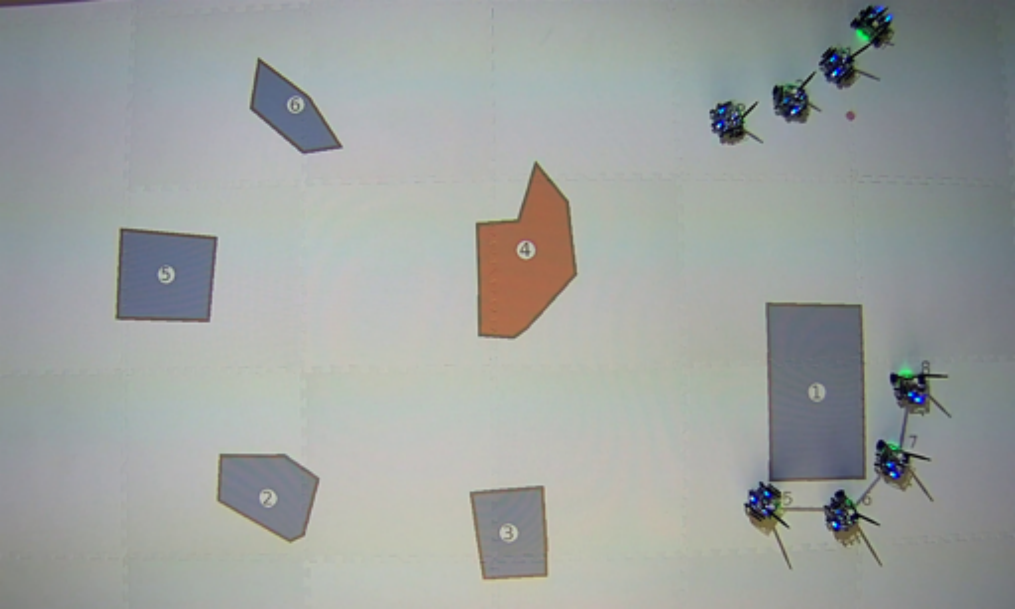
We tested the behavior composition framework described in Section VI on the Securing a Building mission, which was executed on the Robotarium [49]. In Fig. 9, we display selected snapshots of the mission obtained by a camera mounted on the ceiling. In the experiment, differential-drive robots, indexed are deployed in a simulated urban environment composed of buildings, blue polygons indexed . In this experiment, we simulate a maximum sensor range m. Because of the different spatial scales between FIND/ISOLATE phases and RESCUE/FOLLOW-THROUGH phases, the entire mission is divided in two parts. In the first part (Fig. 9(a) to Fig. 9(d)) the experiment is performed at a neighborhood-level scale. The remaining two phases are executed in a zoomed-in environment, which focuses on the one building of interest (Fig. 9(d) to Fig. 9(f)).
During FIND phase (Fig. 9(a) and 9(b)), two groups of robots and investigates preassigned lists of buildings, leaving some agents near the base station (the purple filled dot in the top right corner) if destination building cannot be reached without breaking the connectivity constraints. The red polygon in Fig. 9(b) and 9(c) is the target building after being identified by . During the ISOLATE phase (Fig. 9(c)), maneuvering agents look for the entrance, while the security agents secure the outer perimeter.
During the RESCUE phase (Fig. 9(d) to 9(e)), the agents inside the building, i.e. , localize the target (red dot) using Voronoi coverage (Fig. 9(d)) and escort it to the safe area (red circle) as shown in (Fig. 9(e)). Finally, robots and are left as beacon inside the building, while remaining robots return to the base (Fig. 9(f)).



VIII Conclusion
Sequential execution of multi-robot coordinated behaviors can be employed to solve real-world complex missions. However, sequences of behaviors can be executed only if the robots meet all required communication constraints in finite time. In this paper, we described a distributed framework for the sequential composition of coordinated behaviors designed on finite-time convergence control barrier functions. The resulting composition framework is formulated in the form of a quadratic program, which is solved locally by individual robots. Although the focus of this paper is on coordinated motion, the application of the proposed framework is relevant to other form of autonomous collaborations where the robots need to satisfy prescribed pair-wise proximity requirements that change over time. Finally, a large-scale multi-task scenario, denoted “Securing a Building” mission is proposed as an ideal environment for testing multi-robot techniques.
Appendix A Securing a Building as Benchmark Scenario
Testing the performance of techniques and algorithms for the control of multi-robot systems in real-world scenarios is a challenging task. This is particularly true when addressing novel approaches, as the focus on specific aspects of the problem might obscure all-around performance assessments. To this end, thanks to its modularity, the Securing a Building mission is an ideal testing framework. In this section, we suggest a number of selected research topics, for which this mission could serve as a testing framework when aiming to evaluate performance of new techniques. This appendix is by no mean proposed as a complete list of subjects relevant to multi-robot systems but rather as a discussion to stimulate application of the Securing a Building as a versatile, real-world testing scenario.
Team Assembly
Considerable efforts have been devoted to the development of team composition techniques for heterogeneous robots [51], [52]. Based on the skill set required to solve a particular task, e.g., certain actuation, sensing, locomotion, or communication capabilities, the question is to find a recruitment rule that produces a team capable of delivering the best performance. For instance, in the RESCUE phase, robots capable of opening doors may be required for the maneuvering agents, while agility and communication capabilities might be preferred during the FIND phase.
Communication
In the context of autonomous networked systems, central roles are played by the flow of information between agents, and the infrastructure required for it [53]. A number of questions can be posed in relation to the distribution of agents over a domain, given the constraints of communication systems, such as limited range, power requirements, and privacy of the information.
Unknown Environment
The amount of prior knowledge about the environment plays an important role in the definition of both low-level robot controllers and high-level mission plans. The performance of distributed solutions to the localization and mapping problems [54] can be tested on the Securing a Building. Aspect of interest include balancing between exploitation and exploration of the environment applied, for instance, to the building exploration planning.
Resilience
Failure of the mission can be attributed to factors such as damaged components, sensing errors, communication dropouts, delays, control disturbances, reduction of functionalities due to adversarial attacks, etc. A number of different research thrusts focus on the problem of detecting and responding to faults and malicious attacks in multi-agent and cyber-physical systems [55, 56, 57].
References
- [1] E. Ackerman, “Flying lampshadebots come alive in cirque du soleil performance,” iEEE Spectrum, 2014.
- [2] X. Du, C. E. Luis, M. Vukosavljev, and A. P. Schoellig, “Fast and in sync: Periodic swarm patterns for quadrotors,” arXiv preprint arXiv:1810.03572, 2018.
- [3] M. Santos, Y. Diaz-Mercado, and M. Egerstedt, “Coverage control for multirobot teams with heterogeneous sensing capabilities,” IEEE Robotics and Automation Letters, vol. 3, no. 2, pp. 919–925, 2018.
- [4] D. Shishika and V. Kumar, “Local-game decomposition for multiplayer perimeter-defense problem,” in 2018 IEEE Conference on Decision and Control (CDC). IEEE, 2018, pp. 2093–2100.
- [5] H. Han and R. G. Sanfelice, “A hybrid control algorithm for object grasping using multiple agents,” in 2018 IEEE Conference on Control Technology and Applications (CCTA). IEEE, 2018, pp. 652–657.
- [6] J. Suarez and R. Murphy, “A survey of animal foraging for directed, persistent search by rescue robotics,” in 2011 IEEE International Symposium on Safety, Security, and Rescue Robotics. IEEE, 2011, pp. 314–320.
- [7] D. Zelazo, M. Mesbahi, and M.-A. Belabbas, “Graph theory in systems and controls,” in 2018 IEEE Conference on Decision and Control (CDC). IEEE, 2018, pp. 6168–6179.
- [8] J. Cortés and M. Egerstedt, “Coordinated control of multi-robot systems: A survey,” SICE Journal of Control, Measurement, and System Integration, vol. 10, no. 6, pp. 495–503, 2017.
- [9] J. Lin, A. S. Morse, and B. D. Anderson, “The multi-agent rendezvous problem,” in 42nd IEEE International Conference on Decision and Control (IEEE Cat. No. 03CH37475), vol. 2. IEEE, 2003, pp. 1508–1513.
- [10] W. Ren, R. W. Beard, and T. W. McLain, “Coordination variables and consensus building in multiple vehicle systems,” in Cooperative control. Springer, 2005, pp. 171–188.
- [11] J. L. Ramirez, M. Pavone, and E. Frazzoli, “Cyclic pursuit for spacecraft formation control,” in Proceedings of the American Control Conference, 2009, pp. 4811–4817.
- [12] J. R. Lawton, R. W. Beard, and B. J. Young, “A decentralized approach to formation maneuvers,” IEEE transactions on robotics and automation, vol. 19, no. 6, pp. 933–941, 2003.
- [13] I. Buckley and M. Egerstedt, “Infinitesimally shape-similar motions using relative angle measurements,” in 2017 IEEE/RSJ International Conference on Intelligent Robots and Systems (IROS). IEEE, 2017, pp. 1077–1082.
- [14] J. Cortes, S. Martinez, T. Karatas, and F. Bullo, “Coverage control for mobile sensing networks,” IEEE Transactions on robotics and Automation, vol. 20, no. 2, pp. 243–255, 2004.
- [15] M. Mesbahi and M. Egerstedt, Graph theoretic methods in multiagent networks. Princeton University Press, 2010, vol. 33.
- [16] H. G. Tanner, A. Jadbabaie, and G. J. Pappas, “Flocking in fixed and switching networks,” IEEE Transactions on Automatic control, vol. 52, no. 5, pp. 863–868, 2007.
- [17] S. Nagavalli, N. Chakraborty, and K. Sycara, “Automated sequencing of swarm behaviors for supervisory control of robotic swarms,” in 2017 IEEE International Conference on Robotics and Automation (ICRA). IEEE, 2017, pp. 2674–2681.
- [18] R. K. Ramachandran, J. A. Preiss, and G. S. Sukhatme, “Resilience by reconfiguration: Exploiting heterogeneity in robot teams,” arXiv preprint arXiv:1903.04856, 2019.
- [19] P. Culbertson and M. Schwager, “Decentralized adaptive control for collaborative manipulation,” in 2018 IEEE International Conference on Robotics and Automation (ICRA). IEEE, 2018, pp. 278–285.
- [20] A. Li, L. Wang, P. Pierpaoli, and M. Egerstedt, “Formally correct composition of coordinated behaviors using control barrier certificates,” in 2018 IEEE/RSJ International Conference on Intelligent Robots and Systems (IROS). IEEE, 2018, pp. 3723–3729.
- [21] C. G. Cassandras and S. Lafortune, Introduction to discrete event systems. Springer Science & Business Media, 2009.
- [22] R. C. Arkin, Behavior-based Robotics. MIT press, 1998.
- [23] X. D. Koutsoukos, P. J. Antsaklis, J. A. Stiver, and M. D. Lemmon, “Supervisory control of hybrid systems,” Proceedings of the IEEE, vol. 88, no. 7, pp. 1026–1049, 2000.
- [24] H. Kress-Gazit, M. Lahijanian, and V. Raman, “Synthesis for robots: Guarantees and feedback for robot behavior,” Annual Review of Control, Robotics, and Autonomous Systems, vol. 1, pp. 211–236, 2018.
- [25] M. Srinivasan, S. Coogan, and M. Egerstedt, “Control of multi-agent systems with finite time control barrier certificates and temporal logic,” in 2018 IEEE Conference on Decision and Control (CDC). IEEE, 2018, pp. 1991–1996.
- [26] K. Garg and D. Panagou, “Control-lyapunov and control-barrier functions based quadratic program for spatio-temporal specifications,” arXiv preprint arXiv:1903.06972, 2019.
- [27] P.-J. Meyer and D. V. Dimarogonas, “Hierarchical decomposition of ltl synthesis problem for nonlinear control systems,” IEEE Transactions on Automatic Control, 2019.
- [28] J. Chen, S. Moarref, and H. Kress-Gazit, “Verifiable control of robotic swarm from high-level specifications,” in Proceedings of the 17th International Conference on Autonomous Agents and MultiAgent Systems. International Foundation for Autonomous Agents and Multiagent Systems, 2018, pp. 568–576.
- [29] C. Belta, A. Bicchi, M. Egerstedt, E. Frazzoli, E. Klavins, and G. J. Pappas, “Symbolic planning and control of robot motion [grand challenges of robotics],” IEEE Robotics & Automation Magazine, vol. 14, no. 1, pp. 61–70, 2007.
- [30] E. Klavins and D. E. Koditschek, “A formalism for the composition of concurrent robot behaviors,” in 2000 IEEE International Conference on Robotics and Automation (ICRA), vol. 4. IEEE, 2000, pp. 3395–3402.
- [31] A. Marino, L. Parker, G. Antonelli, and F. Caccavale, “Behavioral control for multi-robot perimeter patrol: A finite state automata approach,” in 2009 IEEE International Conference on Robotics and Automation (ICRA). IEEE, 2009, pp. 831–836.
- [32] M. Vukosavljev, A. P. Schoellig, and M. E. Broucke, “Hierarchically consistent motion primitives for quadrotor coordination,” arXiv preprint arXiv:1905.00500, 2019.
- [33] M. Ji and M. Egerstedt, “Distributed coordination control of multiagent systems while preserving connectedness,” IEEE Transactions on Robotics, vol. 23, no. 4, pp. 693–703, 2007.
- [34] L. Sabattini, C. Secchi, N. Chopra, and A. Gasparri, “Distributed control of multirobot systems with global connectivity maintenance,” IEEE Transactions on Robotics, vol. 29, no. 5, pp. 1326–1332, 2013.
- [35] M. M. Zavlanos, H. G. Tanner, A. Jadbabaie, and G. J. Pappas, “Hybrid control for connectivity preserving flocking,” IEEE Transactions on Automatic Control, vol. 54, no. 12, pp. 2869–2875, 2009.
- [36] Y. Igarashi, T. Hatanaka, M. Fujita, and M. W. Spong, “Passivity-based attitude synchronization in ,” IEEE Transactions on Control Systems Technology, vol. 17, no. 5, pp. 1119–1134, 2009.
- [37] L. Wang, A. D. Ames, and M. Egerstedt, “Multi-objective compositions for collision-free connectivity maintenance in teams of mobile robots,” in 2016 IEEE 55th Conference on Decision and Control (CDC). IEEE, 2016, pp. 2659–2664.
- [38] J. Panerati, M. Minelli, C. Ghedini, L. Meyer, M. Kaufmann, L. Sabattini, and G. Beltrame, “Robust connectivity maintenance for fallible robots,” Autonomous Robots, vol. 43, no. 3, pp. 769–787, 2019.
- [39] V. S. Varadharajan, B. Adams, and G. Beltrame, “The unbroken telephone game: Keeping swarms connected,” in Proceedings of the 18th International Conference on Autonomous Agents and MultiAgent Systems. International Foundation for Autonomous Agents and Multiagent Systems, 2019, pp. 2241–2243.
- [40] P. Twu, P. Martin, and M. Egerstedt, “Graph process specifications for hybrid networked systems,” IFAC Proceedings Volumes, vol. 43, no. 12, pp. 65–70, 2010.
- [41] S. P. Bhat and D. S. Bernstein, “Finite-time stability of continuous autonomous systems,” SIAM Journal on Control and Optimization, vol. 38, no. 3, pp. 751–766, 2000.
- [42] X. Xu, P. Tabuada, J. W. Grizzle, and A. D. Ames, “Robustness of control barrier functions for safety critical control,” IFAC-PapersOnLine, vol. 48, no. 27, pp. 54–61, 2015.
- [43] A. D. Ames, J. W. Grizzle, and P. Tabuada, “Control barrier function based quadratic programs with application to adaptive cruise control,” in 53rd IEEE Conference on Decision and Control. IEEE, 2014, pp. 6271–6278.
- [44] A. D. Ames, S. Coogan, M. Egerstedt, G. Notomista, K. Sreenath, and P. Tabuada, “Control barrier functions: Theory and applications,” 2019 European Control Conference (ECC), pp. 3420–3431, 2019.
- [45] E. Squires, P. Pierpaoli, R. Konda, S. Coogan, and M. Egerstedt, “Composition of safety constraints with applications to decentralized fixed-wing collision avoidance,” arXiv preprint arXiv:1906.03771, 2019.
- [46] R. K. Williams and G. S. Sukhatme, “Observability in topology-constrained multi-robot target tracking,” in 2015 IEEE International Conference on Robotics and Automation (ICRA). IEEE, 2015, pp. 1795–1801.
- [47] J. Aspnes, T. Eren, D. K. Goldenberg, A. S. Morse, W. Whiteley, Y. R. Yang, B. D. Anderson, and P. N. Belhumeur, “A theory of network localization,” IEEE Transactions on Mobile Computing, vol. 5, no. 12, pp. 1663–1678, 2006.
- [48] J. Wagenpfeil, A. Trachte, T. Hatanaka, M. Fujita, and O. Sawodny, “Distributed decision making for task switching via a consensus-like algorithm,” in 2009 American Control Conference. IEEE, 2009, pp. 5761–5766.
- [49] D. Pickem, P. Glotfelter, L. Wang, M. Mote, A. Ames, E. Feron, and M. Egerstedt, “The robotarium: A remotely accessible swarm robotics research testbed,” in 2017 IEEE International Conference on Robotics and Automation (ICRA). IEEE, 2017, pp. 1699–1706.
- [50] “Military operations in urbanized terrain,” US Army Field Manual 90-10, 1975.
- [51] A. Prorok, M. A. Hsieh, and V. Kumar, “Formalizing the impact of diversity on performance in a heterogeneous swarm of robots,” in 2016 IEEE International Conference on Robotics and Automation (ICRA). IEEE, 2016, pp. 5364–5371.
- [52] M. Koes, I. Nourbakhsh, K. Sycara, M. Koes, K. Sycara, I. Nourbakhsh, M. Koes, I. Nourbakhsh, K. Sycara, S. D. Ramchurn et al., “Heterogeneous multirobot coordination with spatial and temporal constraints,” in AAAI, vol. 5, 2005, pp. 1292–1297.
- [53] L. Gupta, R. Jain, and G. Vaszkun, “Survey of important issues in uav communication networks,” IEEE Communications Surveys & Tutorials, vol. 18, no. 2, pp. 1123–1152, 2016.
- [54] C. Forster, S. Lynen, L. Kneip, and D. Scaramuzza, “Collaborative monocular slam with multiple micro aerial vehicles,” in 2013 IEEE/RSJ International Conference on Intelligent Robots and Systems. IEEE, 2013, pp. 3962–3970.
- [55] F. Pasqualetti, A. Bicchi, and F. Bullo, “Consensus computation in unreliable networks: A system theoretic approach,” IEEE Transactions on Automatic Control, vol. 57, no. 1, pp. 90–104, 2011.
- [56] P. Pierpaoli, D. Sauter, and M. Egerstedt, “Fault tolerant control for networked mobile robots,” in 2018 IEEE Conference on Control Technology and Applications (CCTA). IEEE, 2018, pp. 374–379.
- [57] H. Fawzi, P. Tabuada, and S. Diggavi, “Secure estimation and control for cyber-physical systems under adversarial attacks,” IEEE Transactions on Automatic control, vol. 59, no. 6, pp. 1454–1467, 2014.