∎
Clustering Activity-Travel Behavior Time Series using Topological Data Analysis
Abstract
Over the last few years, traffic data has been exploding and the transportation discipline has entered the era of big data. It brings out new opportunities for doing data-driven analysis, but it also challenges traditional analytic methods. This paper proposes a new Divide and Combine based approach to do K-means clustering on activity-travel behavior time series using features that are derived using tools in Time Series Analysis and Topological Data Analysis. Our approach facilitates a case study, where each individual’s daily activity-travel behavior is characterized as a categorical time series consisting of three different levels. Clustering data from five waves of the National Household Travel Survey ranging from 1990 to 2017 suggests that activity-travel patterns of individuals over the last three decades can be grouped into three clusters. Results also provide evidence in support of recent claims about differences in activity-travel patterns of different survey cohorts. The proposed method is generally applicable and is not limited only to activity-travel behavior analysis in transportation studies. Driving behavior, travel mode choice, household vehicle ownership, when being characterized as categorical time series, can all be analyzed using the proposed method.
Keywords:
Activity-travel Patterns Categorical Time Series Divide and Combine Schemes K-means Clustering Persistence Landscapes1 Introduction
Transportation data is exploding in recent years owing to the improved technologies for data collection and storage. A vast amount of data are generated and collected for various purposes. Examples include smartcard data collected by transit operators, mobile phone traces collected by phone carriers, traffic data collected via sensors, smart cameras, global positioning system (GPS) data by road operators, and user’s Wi-Fi locations collected by internet providers. There is an increasing number of studies attempting to leverage big data for answering different transportation-related questions. Studies have sought to use big data for improving traffic management. For example, Jandui Silva 2015 proposed to use data collected by the drivers using apps like Waze and Google Maps to improve urban mobility. Figueiras et al. 2016 proposed to aggregate big data from various sources for implementing dynamic tolling to reduce traffic congestion. Other studies used big data for revealing individuals’ mobility patterns (Calabrese et al. 2013; Candia et al. 2008; Kwan 2000; Huang et al. 2018). For example, Candia et al. 2008 used mobile phone data with time and space resolution to explore collective behavior and detect anomalous events of human activity patterns. Huang et al. 2018 used 7-year transit smartcard data to reveal commute patterns and explore the relationship of job and housing locations of travelers in Beijing, China. When referring to big data analysis, current studies only focus on passively collected data (i.e., phone trace data, smartcard data and sensors data). However, such data has limitations: 1) the datasets do not include the socioeconomic and demographic information of individuals, which are important for understanding the underlying behavior mechanism of individuals’ activity-travel behaviors; 2) the data is not carefully collected to represent a random sample of the population; 3) the data usually requires intensive processing before being used for analysis (Calabrese et al. 2013). On the other side of the spectrum we have traditional surveys that overcome these limitations. Due to the high expense of conducting surveys, most surveys only collect data from a small sample within limited temporal and spatial scales. However, the National Household Travel Survey increased in recent years and it is the largest travel survey that collects detailed trip information. As aforementioned, actively collected survey data shows advantages for analyzing activity-travel patterns. It not only contains activity-travel behavior of each individual, but also includes socioeconomic and demographic information for revealing the underlying mechanisms of the behavior of individuals.
Understanding the relationship between individuals’ activity-travel behaviors and their socioeconomic and demographic characteristics can help transportation planners promote efficient solutions and policies for a given region. When analyzing activity-travel behavior using survey data, researchers tend to focus on one or two aspects of activity and travel (i.e., trip rate, mode choice, or activity type). They often ignore the temporal dimension of activity-travel behaviors (i.e., timing, duration and sequential order of activity and travel). One way to incorporate these is through a categorical time series characterization (Wilson 2001; Recker et al. 1985; Shoval and Isaacson 2007; Zhang et al. 2018; Goulias 1999). Each data point of the time series represents a minute spent in either travel or activity over the course of a day.
It is useful to first cluster the categorical time series, separating individuals into groups of distinct temporal behaviors and then explore the relationship between the temporal behaviors and their demographic characteristics. Two types of clustering methods have been widely adopted, the sequence alignment method (Joh et al. 2001; Wilson 2001; Recker et al. 1985; Pas 1988; Shoval and Isaacson 2007; Zhang et al. 2018) and the Markov modeling approach (Goulias 1999). The sequence alignment method was first developed in molecular biology for calculating the sequential similarity between DNA strings. The method is based on the Levenshtein distance, also called the Edit distance, which is defined as the smallest number of changes made in the elements to equalize two sequences (Joh et al. 2001). The method is very computationally intensive, and so it has only been applied for analyzing small datasets. The Markov model is also useful for characterizing categorical time series and estimates the probability of transitioning from an activity-travel model at time to another activity at time . The Markov model is generally most suitable when the time series patterns change periodically.
We propose an approach that constructs useful features from time series using frequency domain properties and Topological Data Analysis (TDA)11 1 A brief review is provided in the appendix. For details on TDA, see Edelsbrunner and Harer 2010; Wang et al. 2018. Our approach then clusters the series into groups based on these features. That is, we propose a sequence alignment method based on the dissimilarity between series using TDA based features. In order to attain computational speed in applying this approach, we propose a divide and combine scheme for the implementation.
The rest of the paper is organized as follows. Section 2 shows how we can construct useful features of time series using TDA. In Section 3, we discuss K-means clustering of a large number of time series based on these features, by using a divide and combine scheme to handle the computational burden. Both Sections 2 and 3 provide generic descriptions that can be used with any set of categorical time series. Section 4 discusses this approach on a case study on diurnal activity-travel behavior of a large number of participants from the National Household Travel Survey (NHTS)/National Personal Travel Survey (NPTS). Section 5 presents a summary of our contributions and ideas for future research. The appendix provides a brief review of TDA and the persistence landscape construction.
2 TDA Based Features of Categorical Time Series
Section 2 describes feature extraction from categorical time series using TDA on their frequency domain representations. Let , and denote a large set of categorical time series, each of length and each assuming levels. The feature extraction from each categorical time series consists of two steps.
In the first step, we convert the time series to their frequency domain representations, the Walsh-Fourier transforms (WFT), which are useful in representing “sequency patterns” in categorical time series (Stoffer 1991). We use an efficient algorithm developed by Shanks 1969 to compute the fast WFT using discrete, orthogonal Walsh functions generated by a multiplicative iteration equation. Walsh functions constitute a set of piecewise constant functions which assume a value of or on sub-intervals of time defined by dyadic fractions. Although the fast WFT captures the sequency properties of the time series, its usefulness as a feature in clustering the time series may be mitigated when a time series has low (rather than high) sequency patterns. It is useful to retain the dominant sequency features of the WFT, while removing redundancies.
For this purpose, in the second step of the feature construction, we convert the WFT of the time series into a first-order persistence landscape (Bubenik 2015), which is a summary statistic in topological data analysis (TDA) and is easy to compute and combine with tools from statistics and machine learning. The appendix gives a brief review of concepts in TDA, which is being increasingly explored for analyzing big, complex data (Wang et al. 2018; Stolz et al. 2017), and in particular, a description of the first-order persistence landscape corresponding to a function. The persistence landscape of the WFT will be useful to pull up the strongest temporal patterns in the categorical time series, and will be employed as features in the clustering algorithm. The two-step procedure is described below.
Step 2.1. Fast Walsh-Fourier Transform of a Categorical Time Series. Construct the fast WFT using the method of Shanks 1969 to decompose the th time series into a sequence of Walsh functions, each representing a distinctive binary sequency pattern. If the time series length is not a power of , let denote the next power of . For example, if , then . Use zero-padding to obtain a time series of length , i.e., set .
For , let denote the th sequency. Let denote the -th Walsh function value in sequency . Walsh functions are iteratively generated as follows (Shanks 1969):
| (1) | |||||
where denotes the integer part of . For more details on Walsh functions, please refer to Stoffer 1991.
The Walsh-Fourier Transform (WFT) of is computed as
| (2) |
The length of is . We use C++ code to compute the fast WFT and its computational complexity is (Shanks 1969).
Step 2.2. Persistence Landscape Corresponding to a WFT. We construct a first-order persistence landscape (see the appendix for a brief review) corresponding to the WFT of the time series as follows. Denote the minimum and maximum of the WFT values of the time series by
Let
denote the minimum and maximum values of the WFTs across all time series.
We construct the first-order persistence landscape of length , for a time series indexed by . Usually, is chosen to be considerably smaller than the length of the time series for computational speed, while not making it too small to make the persistence landscape from the WFT ineffective to capture essential features of the time series. We have chosen based on the empirical observation that it captures the strongest temporal patterns in the activity-travel categorical time series.
The first-order persistence landscape of is obtained for as
| (3) |
where
and denotes the positive part of a real number . For and , the are piecewise linear functions that constitute features constructed for each of the time series and will be input into a clustering algorithm described in the next section.
3 Divide and Combine K-means Clustering
We use the persistence landscapes for and as features to cluster the series into homogeneous groups via the K-means algorithm. When is large, we can gain efficiency by operating the algorithm in parallel on multiple processors. We use a divide and combine approach for implementing the K-means algorithm using Message Passing Interface (MPI) for parallel computing in C++. This significantly reduces the computing time and automatically resolves the limited memory and power restrictions of a single computer. We use the University of Connecticut (UConn) High Performance Computing (HPC) cluster with cores. The nodes consist of mixed four versions of Xeon processors (Xeon E5-2650, Xeon E5-2680 v2, Xeon E5-2690 v3, and Xeon E5-2699 v4), each having 36 cores and 156 GB; since we use cores, we would receive nodes with different configurations. The procedure consists of several steps.
- 3.1.
Data Division into Processors. Denote the ordering of the categorical time series as , . We randomly divide the full data set of size categorical time series into sets, so that each set consists of time series, which is a manageable number to analyze (in parallel) on each of processors on the UConn HPC cluster. The division is done by randomly sampling the indices of the time series without replacement and then assigning the first time series to the first processor, successive series to the second processor, etc. Usually, we would assume that and assign the remaining time series to the -th processor. The random sampling orders of the indices are saved into the vector .
- 3.2.
Feature Extraction Within Each Processor.
- 3.2.1.
Obtain the WFT of each categorical time series, following Step 2.1.
- 3.2.2.
Convert the WFT to a first-order persistence landscape, following Step 2.2.
- 3.2.1.
- 3.3.
K-means Algorithm on Parallel Processors. We implement the K-means algorithm independently on each processor , using as features the persistence landscapes of length from each time series. Select the number of clusters . The entire algorithm will be run for different choices of . We also set the maximum number of iterations to be , chosen to be . We set the iteration counter at . We implement the following steps.
- 3.3.1.
Set . Generate centroids of each of the clusters, each of length , as follows:
- (i)
if , generate the centroids for each of the clusters randomly on each processor which corresponds to time series. Each of the centroid components are drawn from a Uniform distribution, where and .
- (ii)
if , use the centroids sent by the master processor at the end of Step 3.3.3.
Run the K-means algorithm independently on each processor (note that the K-means algorithm itself includes iterations by default). For and iteration , save into the set of -dimensional centroids from cluster , for . Set a flag for each processor as follows:
- (i)
if , set a flag for each .
- (ii)
if , set if cluster labels change after the K-means algorithm on processor , else set .
- (i)
- 3.3.2.
For , processor returns to the master processor the set of centroids and the flag . For any iteration ,
- (i)
if at least one of the flags is set at 1, the procedure of centroid selection must be iterated further; go to Step 3.3.3.
- (ii)
if all the flags are set at 0, the selection of centroids is complete; go to Step 3.4.
- (i)
- 3.3.3.
The master processor applies the same K-means algorithm with clusters on the centroids , , and updates the new set of centroids as , . Note that each is used an input into the K-means on centroids and is the set of centroids after K-means. The master processor then sends the set back to all processors. For example, when and , the master processor receives centroids from all processes, i.e., , and generates the set from the K-means on centroids algorithm, which is broadcast to all processors, so that each of them may use these centroids in Step 3.3.1.
- 3.3.1.
- 3.4.
Combine Results from Processors. All processors return cluster labels , where denotes the cluster label for the -th subject. Each processor also returns to the master processor its Within-Cluster Sum of Squares defined as
where is the indicator function. The master processor saves the cluster labels from the processors in order, . Let
(4) denote the Total Within Cluster Sum of Squares.
Figure 1 gives an overview of all the steps. The final outputs from the entire procedure are: the random sampling orders ; the WFT from each processor; the first-order persistence landscapes from each processor; the cluster labels ; and the WCSS. For doing interpretations by using the original time series with the cluster labels, , we can use on the raw time series again to make the ordering match with .

4 Case Study: Analysis of Within-Day Activity-Travel Patterns
In this section, we present a detailed case study of applying our TDA based clustering procedure to activity-travel patterns from participants in multiple waves of National Household Travel Survey data ranging from 1990 to 2017. Following a motivation of this case study in section 4.1, we provide a detailed data description in section 4.2 and the study design in section 4.3. In section 4.4, we give a discussion of the divide and conquer algorithm that uses TDA derived feature clustering described in Sections 2 and 3. Section 4.5 discusses the interpretation of results.
4.1 Motivation of the Transportation Case Study
As mentioned in the introduction, the large-scale actively collected travel survey data provides tremendous opportunities for conducting data-driven analysis for understanding activity-travel behaviors. The algorithm described in Sections 2 and 3 is applied to identify clusters of individuals based on their intra-day activity-travel patterns. In particular, we are interested in investigating whether activity-travel behavior varies across different generation cohorts, employment status, income, or gender. These four factors have been acknowledged in the literature as strongly associated with activity-travel behavior. To this end, the primary objective of this case study is to use the proposed approach to identify clusters of individuals based on their daily activity-travel behaviors. Subsequently, the association of activity-travel behaviors and four influence factors (generational cohorts, gender, income, and employment status) is explored by investigating characteristics within each cluster and contrasting them between clusters. Our contribution is the ability to handle state-of-the-art statistical analysis of large datasets using the divide and combine approach, as well as to construct features that garner topological features of categorical time series.
4.2 Description of the Activity-Travel Data
The data for this study was obtained by combining multiple waves of the National Household Travel Survey (NHTS) /National Personal Travel Survey (NPTS). More specifically, the 2001, 2009 and 2017 waves of the NHTS and 1990, and 1995 waves of the NPTS were combined. Each wave of the NHTS/NHPS dataset provides information about the daily activity-travel behaviors of a nationally representative sample. The survey has been sponsored by the Federal Highway Administration and conducted periodically since 1969.
Datasets are currently available for 1983, 1990, 1995, 2001, 2009 and 2017 and we only used the datasets from five waves of NHTS/NPTS including 1990, 1995, 2001, 2009 and 2017. The 1983 survey was excluded due to data quality issues.
The surveys asked each sampled participant to report all trips he/she made during a designated 24-hour time period, from 4 a.m. of one day until 4 a.m. of the next day, yielding a time series of length minutes per respondent. Table 1 shows some basic information about this data. Column 1 shows the name of the survey while Column 2 shows the number of available respondents under each survey. For our analysis, we focus on adults (i.e., 18 years or older) who reported their activity-travel on a typical weekday (Tuesday, Wednesday, or Thursday), and their counts are shown in Column 3 of the table. The number of respondents across all surveys for our analysis is . In addition to the activity-travel behavior information, socioeconomic and demographic information of the respondents (i.e., age, gender, employment status, etc.) are also provided for each survey.
| Data Source | Full Survey | Selected Adults |
|---|---|---|
| 1990 NHTS | 48385 | 9769 |
| 1995 NHTS | 95360 | 20997 |
| 2001 NHTS | 160758 | 44201 |
| 2009 NHTS | 308901 | 84366 |
| 2017 NHTS | 264234 | 91549 |
| Total | 877638 | 250882 |
We denote as the number of participants in survey wave for . Then, . Rather than counting each participant once, we will follow NHTS and assign a “weight” to the th participant, . The weighting scheme is used in order to produce valid population-level estimates by trying to reduce nonresponse bias and sampling bias. This procedure is standard in the analysis of household surveys, including steps of calculating base weights, adjusting the base weights for eligibility and nonresponse, and further poststratifying the adjusted weights to external source data (Shelley Brock Roth 2017); see Table 2. The entries in the table indicate no observations. Specifically, there are no Millennials in Waves 1 and 2 because they were not adults at that time yet. There is no Government Issue Generation in Wave 5 as well.
Different generations are defined based on people’s birth year: Government Issue (GI) Generation (birth year 1901 to 1924); Silent Generation (birth year 1925 to 1943); Baby Boomers (birth year 1944 to 1964); Generation X (birth year 1965 to 1981); Millennials (birth year 1982 to 2000).
| Wave1 | Wave2 | Wave3 | Wave4 | Wave5 | |
| GI | 4101984 | 3607945 | 2993436 | 900313 | 0 |
| Silence Generation | 10805726 | 10766706 | 12304352 | 9329861 | 5895241 |
| Baby Boomer | 22337829 | 23282036 | 27896189 | 27303881 | 28444900 |
| Generation X | 7885177 | 13484379 | 24599990 | 25747942 | 26858832 |
| Millennial | 0 | 0 | 2614342 | 12573553 | 29109232 |
| Worker | 33352378.6 | 37299955.77 | 52174455.13 | 53247605.7 | 61458579.48 |
| Non-worker | 11778337.55 | 13841109.19 | 18232436.39 | 22593569.93 | 28846987.6 |
| Male | 22772337 | 25938351 | 34993077 | 37756891 | 44694301 |
| Female | 22358379 | 25202714 | 35415231 | 38098659 | 45558163 |
4.3 Study Design
We use three activity-travel types to characterize an individual’s daily pattern. These include (a) in-home activity, (b) out-of-home activity, and (c) travel. This information is derived by consolidating detailed trip purpose categories provided by the survey. For each respondent and for each minute , we define the categorical time series with levels as follows:
| (5) |
Figure 2 shows the proportions of these three categories on the different survey waves. The title for each plot shows the year of the wave and the number of respondents. In general, all waves exhibit similar profiles, with the “Home” category having the highest proportion of respondents in the beginning and the end, while the “Out of Home” category is dominant during the middle of the day.

Figure 3 shows the categorical time series for nine randomly selected respondents. The x-axis shows the time in minutes from 4 am on a given day until 4 am of the next day, for a total of minutes. The y-axis shows in which of the three categories the respondent is at each minute . The figure shows that several respondents have normal behaviors, i.e., they go out in the early morning ( is 5:00 to 8:00 am), spend the daytime outside, and return home in the late afternoon ( is 6:00 to 9:00 pm). There is another kind of activity-travel pattern where people stay at home most of the time, except for a couple of hours during the afternoon ( is 3:00 to 7:00 pm).

4.4 Clustering Respondents by the Divide and Combine Scheme
We employ the divide and combine scheme described in Sections 2 and 3. We use Step 3.1 to divide the respondents into sets. The first sets have respondents each, while the last set has respondents. Each set is assigned to a different processor on the UConn cluster, as described in Section 3. Within each of the processors, we extract the first-order persistence landscape corresponding to the WFT of each series.
For a given number of clusters , we carry out the K-means algorithm in parallel on the processors (see Step 3.3), in interaction between these processors and the main processor. We then combine the results (see Step 3.4) to arrive at the final stage of clustering the respondents into groups.
In practice, the number of clusters is unknown. To select , we use WCSS, a measure of overfitting defined in equation (4). Table 3 shows the values of WCSS and computation times for each value of ranging from to . We separate the time cost for the feature extraction and K-means via using UConn HPC cluster with nodes/processors.
| No. | WCSS | seconds (FE + K-means) |
|---|---|---|
| 9.2E4 | 3.3+0.8 | |
| 4.5E4 | 3.3+1.09 | |
| 3.4E4 | 3.3+2.82 | |
| 2.7E4 | 3.3+2.5 |
The procedure takes only a few seconds to construct the features and complete the clustering, which indicates that the method is highly computationally effective. . Figure 4 plots the WCSS versus the number of clusters . Using the Elbow method (Thorndike 1953; Ketchen and Shook 1996), we see that the plot selects clusters.
4.5 Interpretation of Results
Figure 5 also shows the proportion of each category over minutes. Three clusters were obtained by applying the proposed method. () respondents fall into cluster 1, () respondents fall into cluster 2, and () respondents fall into cluster 3. Cluster 1 contains adults staying at home most of the time so will be named “C1-in home”; Cluster 2 is named “C2-night discretionary” as most of the adults in the cluster would stay in the “Out of Home” category until the end of the survey period; Cluster 3 is named “C3-home and work” as people in the Cluster 3 would stay in the “Out of Home” category during the daytime and stay in the “Home” category at night.

We are interested in four demographic variables as they are closely related to activity-travel patterns in the literature, generations (GI Generation, Silent Generation, Baby Boomers, Generation X, Millennials), gender (male, female), income (25k-, 25k-55k, 55k-75k, 75k-100k, 100k+), and employment (worker, non-worker). In the following, we explore the activity-travel patterns of different survey periods by considering these attributes.
In Figure 6, we can see that (a) most of adults in the GI generation are in “C1-in home”, which indicates that they are aged; (b) the adults of Silent Generation are moving from “C3-home and work” to “C1-in home”, which can be the sign of them aging, the same as the Baby Boomers; (c) the majority of both of Generation X and Millennials are in cluster “C3-home and work”, which are workers and students.

We then explore the composition of different clusters over the different survey periods, as functions of demographic variables, like gender, employment and income.
In general, Figure 7 shows that majority of both male and female are in cluster “C3-home and work”, and the proportions of both of male and femalein cluster “C1-in home” increase. What is more, starting from 2009, the distributions of females in cluster “C1-in home” and females in cluster “C3-home and work” are about the same, which indicates that there is a trend of female spending more time at home.

Figure 8 shows a strong connection between the employment types and the clusters. If people are workers, majority of them are in the cluster “C3-home and work”, and the majority of non-workers are in the cluster “C1-in home”. On the other hand, it is interesting to see that an increasing trend of workers in the cluster “C1-in home” and a decreasing trend of workers in the “C3-home and work”, which indicates that there are more workers starting to work from home.

Figure 9 shows the composition for different income levels. It is interesting to see that the middle income levels (from to ) have an increasing trend of cluster “C1-in home” over years and a decreasing trend of the “C3-home and work”. Combining with Figure 8 above, it means that the increasing trend of workers working at home are in the middle income level.

5 Summary and Discussion
In order to understand the relationship between individuals’ activity-travel behaviors and their demographic characteristics using actively collected “big” survey data, a new sequence alignment method to cluster the temporal behaviors is proposed. The proposed method is demonstrated using data from NHTS to identify clusters of activity-travel patterns. The method uses TDA to construct a first-order persistence landscape which is then used as a feature for clustering. The proposed method has been implemented in C++ and the code is posted on Github.
It must be pointed out that there are a large number of other factors that are also highly related to daily activity-travel behaviors, such as, age, life cycle, built environment, etc. however, given the methodology focus of this study, a more comprehensive investigation is left to a follow up paper.
Last but not least, the aggregation procedure of converting features is only focused on the first-order persistence landscape, which is essentially the combination of the maximum and minimum of the Walsh-Fourier Transforms. It is an appropriate approach when the raw time series is relatively simple, not containing too many significant patterns. If the activity-travel patterns are more complex, like a salesman’s business day, it could be meaningful to construct higher order persistence landscapes, which will be related to a set of local maxima and minima of the Walsh-Fourier Transforms. This will be the subject of future research.
Appendix: TDA and the First-order Persistence Landscape
We start with a brief review of Topological Data Analysis (TDA), which is now an emerging area for analyzing big data with complex structures. Using computational homology, TDA is aimed at analyzing the topological features of data and representing these features using low dimensional representations (Carlsson 2009). The input to TDA is often a set of data points (point cloud) or a function, and persistence homology distills essential topological features in the data, which can then be used together with suitable dissimilarity measures to identify patterns in the data sets. We discuss TDA on functions, which is the approach developed in Sections 2 and 3.
Computational Procedure for TDA on Functions
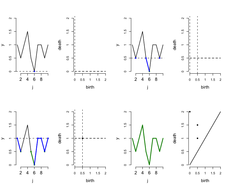
We look at the method to construct persistence diagrams on functions by using the sublevel set filtration. Figure 10 shows the simple procedure of extracting a persistence diagram from a function. Suppose and let the sublevel set be . TDA is used to construct the persistence diagram based on .
- (i)
When , a connected component is identified (marked as a blue dot, which is the oldest connected component). The vertical slash line of the second plot records the “birth time ” and the horizontal slash line indicates . There is no point on the birth/death plot, since no connected components died at .
- (ii)
When , there are two more connected components coming out (indicated in blue); the blue dot in the middle with a blue line connecting it to the dark green dot indicates that the oldest connected component “enlarges” and is “still alive”. The other black vertical slash line in the second plot gives the “birth time” for the other two new connected components. There is no connected component dead yet, and hence no points are shown on the birth/death plot.
- (iii)
When , all old components “enlarge” and there is one newer component “killed” by the older one. Therefore, there is a “black dot with birth and death ” shown on the second plot.
- (iv)
When , the last component is “killed, birth , death ”, which is the black dot on the location . The other black dot corresponding to of the second plot tells the “birth and death” of another connected component.
First-Order Persistence Landscape
First, in the persistence diagram obtained by using the sublevel set filtration, the furthest point away from the diagonal line is always born at the minimum value of the function and dies at the maximum value of the function.
Second, referring to the definition of persistence landscape in Section 2.3 from Bubenik 2015, given a persistence diagram , the first-order persistence landscape is
where is a real number. Because the persistence diagram uses a sublevel set filtration, it has the point . For all that belong to the persistence diagram, . Therefore, for any real number , and , which implies that
which in turn implies that
Finally, let and taking grids , we have
where,
These expressions will be used on the WFT function obtained from each time series in Section 2.
Conflict of interest
The authors declare that they have no conflict of interest.
References
- Bubenik (2015) Bubenik P (2015) Statistical topological data analysis using persistence landscapes. J Mach Learn Res 16(1):77–102
- Calabrese et al. (2013) Calabrese F, Diao M, Lorenzo GD, Ferreira J, Ratti C (2013) Understanding individual mobility patterns from urban sensing data: A mobile phone trace example. Transportation Research Part C: Emerging Technologies 26:301 – 313
- Candia et al. (2008) Candia J, González MC, Wang P, Schoenharl T, Madey G, Barabási AL (2008) Uncovering individual and collective human dynamics from mobile phone records. Journal of Physics A: Mathematical and Theoretical 41(22):224015
- Carlsson (2009) Carlsson G (2009) Topology and data. Bulletin of the American Mathematical Society 46(2):255–308
- Edelsbrunner and Harer (2010) Edelsbrunner H, Harer J (2010) Computational Topology. An Introduction. American Mathematical Society
- Figueiras et al. (2016) Figueiras P, Silva R, Ramos A, Guerreiro G, Costa R, Jardim-Goncalves R (2016) Big data processing and storage framework for its: A case study on dynamic tolling. ASME 2016 International Mechanical Engineering Congress and Exposition
- Goulias (1999) Goulias KG (1999) Longitudinal analysis of activity and travel pattern dynamics using generalized mixed markov latent class models. Transportation Research Part B: Methodological 33(8):535 – 558
- Huang et al. (2018) Huang J, Levinson D, Wang J, Zhou J, Wang Zj (2018) Tracking job and housing dynamics with smartcard data. Proceedings of the National Academy of Sciences 115(50):12710–12715
- Jandui Silva (2015) Jandui Silva LLVSFF Bárbara França (2015) Towards smart traffic lights using big data to improve urban traffic. SMART 2015: The Fourth International Conference on Smart Systems, Devices and Technologies
- Joh et al. (2001) Joh CH, Arentze T, Timmermans H (2001) Pattern recognition in complex activity travel patterns: comparison of euclidean distance, signal-processing theoretical, and multidimensional sequence alignment methods. Transportation Research Record: Journal of the Transportation Research Board (1752):16–22
- Ketchen and Shook (1996) Ketchen DJ, Shook CL (1996) The application of cluster analysis in strategic management research: an analysis and critique. Strategic management journal 17(6):441–458
- Kwan (2000) Kwan MP (2000) Interactive geovisualization of activity-travel patterns using three dimensional geographical information systems: a methodological exploration with a large data set. Transportation Research Part C: Emerging Technologies 8:185–203
- Pas (1988) Pas EI (1988) Weekly travel-activity behavior. Transportation 15(1):89–109
- Recker et al. (1985) Recker WW, McNally MG, Root GS (1985) Travel/activity analysis: Pattern recognition, classification and interpretation. Transportation Research Part A: General 19(4):279 – 296
- Shanks (1969) Shanks JL (1969) Computation of the fast walsh-fourier transform. IEEE Trans Comput 18(5):457–459
- Shelley Brock Roth (2017) Shelley Brock Roth JD Yiting Dai (2017) 2017 nhts weighting report. National Household Travel Survey
- Shoval and Isaacson (2007) Shoval N, Isaacson M (2007) Sequence alignment as a method for human activity analysis in space and time. Annals of the Association of American Geographers 97:282 – 297
- Stoffer (1991) Stoffer DS (1991) Walsh-fourier analysis and its statistical applications. Journal of the American Statistical Association 86(414):461–479
- Stolz et al. (2017) Stolz BJ, Harrington HA, Porter MA (2017) Persistent homology of time-dependent functional networks constructed from coupled time series. Chaos: An Interdisciplinary Journal of Nonlinear Science 27(4):047410
- Thorndike (1953) Thorndike RL (1953) Who belongs in the family. Psychometrika pp 267–276
- Wang et al. (2018) Wang Y, Ombao H, Chung MK (2018) Topological data analysis of single-trial electroencephalographic signals. The annals of applied statistics 12(3):1506
- Wilson (2001) Wilson C (2001) Activity patterns of canadian women: Application of clustalg sequence alignment software. Transportation Research Record 1777(1):55–67
- Zhang et al. (2018) Zhang A, Kang JE, Axhausen K, Kwon C (2018) Multi-day activity-travel pattern sampling based on single-day data. Transportation Research Part C: Emerging Technologies 89:96 – 112