跳到论文正文
W Papers独立论文阅读器 arXiv:1907.07470 论文正文 计算阅读时间 · 0%
引用这篇论文根据当前论文元数据生成,正式投稿前建议核对。


License: CC BY 4.0
arXiv:1907.07470v2 [math.AP] 10 Dec 2019

Inhomogeneous domain walls in spintronic nanowires

L. Siemer Note: Universität Bremen, lars.siemer@uni-bremen.de; Corresponding author    I. Ovsyannikov Note: Universität Hamburg, Lobachevsky State University of Nizhny Novgorod    J.D.M. Rademacher Note: Universität Bremen
August 11, 2026
Abstract

In case of a spin-polarized current, the magnetization dynamics in nanowires are governed by the classical Landau-Lifschitz equation with Gilbert damping term, augmented by a typically non-variational Slonczewski term. Taking axial symmetry into account, we study the existence of domain wall type coherent structure solutions, with focus on one space dimension and spin-polarization, but our results also apply to vanishing spin-torque term. Using methods from bifurcation theory for arbitrary constant applied fields, we prove the existence of domain walls with non-trivial azimuthal profile, referred to as inhomogeneous. We present an apparently new type of domain wall, referred to as non-flat, whose approach of the axial magnetization has a certain oscillatory character. Additionally, we present the leading order mechanism for the parameter selection of flat and non-flat inhomogeneous domain walls for an applied field below a threshold, which depends on anisotropy, damping, and spin-transfer. Moreover, numerical continuation results of all these domain wall solutions are presented.

1 Introduction

Magnetic domain walls (DWs) are of great interest both from a theoretical perspective and for applications, especially in the context of innovative magnetic storages [1]. Recent developments in controlled movement of DWs via spin-polarized current pulses in nanomagnetic structures, in particular in nanowires, are thought to lead to a new class of potential non-volatile storage memories, e.g. racetrack memory [1, 2, 3, 4]. These devices make use of the fact that spin-transfer driven effects can change the dynamics in sufficiently small ferromagnetic structures (e.g. nanowires), where regions of uniform magnetization, separated by DWs, can appear [5, 6, 7]. This motivates further studies of the existence of magnetic domains and their interaction with spin-polarized currents as a building block for the theory in this context. In this paper we take a mathematical perspective and, in a model for nanomagnetic wires, rigorously study the existence of DWs. This led us to discover an apparently new kind of DWs with a certain inhomogeneous and oscillatory structure as explained in more detail below.

The description of magnetization dynamics in nanomagnetic structures, governed by the Landau-Lifschitz-Gilbert (LLG) equation, is based on works by Berger and Slonczewski assuming a spin-polarized current [8, 9]. In the presence of a constant applied field and a spin-polarized current, the dynamics driven by the joint action of magnetic field and spin torque can be studied by adding a spin-transfer term in the direction of the current (current-perpendicular-to-plane (CPP) configuration). In case of a spatially uniform magnetization, the resulting Landau-Lifschitz-Gilbert-Slonczewski (LLGS) equation for unit vector fields (m1,m2,m3)=𝒎=𝒎⁡(x,t)∈𝕊2(m_{1},m_{2},m_{3})=\boldsymbol{m}=\boldsymbol{m}(x,t)\in\mathbb{S}^{2} (cf. Figure 1) reads

∂t𝒎−α𝒎×∂t𝒎=−𝒎×𝒉eff+𝒎×(𝒎×𝑱).\partial_{t}\boldsymbol{m}-\alpha\boldsymbol{m}\times\partial_{t}\boldsymbol{m}=-\boldsymbol{m}\times\boldsymbol{h}_{\textnormal{eff}}+\boldsymbol{m}\times\left(\boldsymbol{m}\times\boldsymbol{J}\right). (LLGS)

with effective field 𝒉eff\boldsymbol{h}_{\textnormal{eff}}, Gilbert damping factor α>0\alpha>0, and the last term is the so-called polarized spin transfer pseudotorque.

Note that the above equation reduces to the LLG equation for 𝑱≡0\boldsymbol{J}\equiv 0, see §2 for more details.

In this paper we consider the axially symmetric case and set

𝒉eff≔∂x2𝒎+𝒉−μ​m3​𝒆3,𝑱≔β1+ccp​m3​𝒆3,\boldsymbol{h}_{\textnormal{eff}}\coloneqq\partial^{2}_{x}\boldsymbol{m}+\boldsymbol{h}-\mu\,\textnormal{m}_{3}\,\boldsymbol{e}_{3}\,,\quad\boldsymbol{J}\coloneqq\frac{\beta}{1+c_{\textnormal{cp}}m_{3}}\boldsymbol{e}_{3}\,, (1)

where 𝒉=h​𝒆3\boldsymbol{h}=h\,\boldsymbol{e}_{3} with a uniform and time-independent field strength h∈ℝh\in\mathbb{R}, and m3=⟨𝒎,𝒆3⟩\textnormal{m}_{3}=\langle\boldsymbol{m},\boldsymbol{e}_{3}\rangle, 𝒆3∈𝕊2\boldsymbol{e}_{3}\in\mathbb{S}^{2}. This effective field 𝒉eff\boldsymbol{h}_{\textnormal{eff}} also includes the diffusive exchange term ∂x2𝒎\partial_{x}^{2}\boldsymbol{m}, the uniaxial anisotropy and demagnetization field. The specific here with parameter μ∈ℝ\mu\in\mathbb{R} derives from a first order approximation in the thin film/wire limit for a uniformly magnetized body [6, 10]. In the axially symmetric structure, β≥0\beta\geq 0 and ccp∈(−1,1)c_{\textnormal{cp}}\in(-1,1) describe the strength of the spin-transfer and the ratio of the polarization [7, 11]. The spin-transfer torque term may provide energy to the system under certain conditions and counterbalance dissipation associated to the Gilbert damping term, which gives rise to coherent non-variational dynamics, see e.g. [12].

Notably, for β=0\beta=0 one obtains the LLG-equation that does not account for spin transfer effects. Moreover, as shown in [12], this also holds up to parameter change in case ccp=0c_{\textnormal{cp}}=0. Hence, solutions to the LLGS equation for β=0\beta=0 or ccp=0c_{\textnormal{cp}}=0 are also solutions to the LLG equation, so that all the analytical as well as numerical results for ccp=0c_{\textnormal{cp}}=0 in this paper directly transfer to the LLG equation.

Refer to caption
(a)
Refer to caption
(b)
Refer to caption
(c)
Figure 1: Homogeneous DW profile (q≡0q\equiv 0) with α=0.5,β=0.1,μ=−1,h=50,ccp=0\alpha=0.5,\beta=0.1,\mu=-1,h=50,c_{\textnormal{cp}}=0. (a) (m2,m3)(m_{2},m_{3})-profile. (b) Projection onto 𝕊2\mathbb{S}^{2}. (c) Zoom-in on m1m_{1} (blue solid) and m2m_{2} (red dashed).

A key ingredient for the separation of uniformly magnetized states in space are interfaces between two magnetic domains. The most coherent form of such interfaces in the uniaxial setting are relative equilibria with respect to translation and rotation symmetry of the form

𝒎⁡(ξ,t)=𝒎0​(ξ)​ei​φ​(ξ,t),where ​ξ=x−s​t​ and ​φ​(ξ,t)≔ϕ⁡(ξ)+Ω​t,\boldsymbol{m}(\xi,t)=\boldsymbol{m}_{0}(\xi)\mathrm{e}^{\mathrm{i}\varphi(\xi,t)},\quad\textnormal{where }\xi=x-st\textnormal{ and }\varphi(\xi,t)\coloneqq\phi(\xi)+\Omega t,

with speed ss and frequency Ω\Omega. Here the complex exponential acts on 𝒎0∈𝕊2\boldsymbol{m}_{0}\in\mathbb{S}^{2} by rotation about the 𝒆3\boldsymbol{e}_{3}-axis, i.e., the azimuth, and in spherical coordinates we can choose 𝒎0​(ξ)=(sin⁡(θ⁡(ξ)),0,cos⁡(θ⁡(ξ)))\boldsymbol{m}_{0}(\xi)=\left(\sin(\theta(\xi)),0,\cos(\theta(\xi))\right) with altitude angle θ\theta.

We refer to such solutions with 𝒎0​(ξ)→±𝒆3\boldsymbol{m}_{0}(\xi)\to\pm\boldsymbol{e}_{3} as ξ→±∞\xi\to\pm\infty or ξ→∓∞\xi\to\mp\infty as domain walls. A first classification of DWs is based on the local wavenumber q:=ϕ′q:=\phi^{\prime}, which determines ϕ\phi uniquely due to the axial rotation symmetry and satisfies

q​(ξ)=⟨(m1′,m2′),(−m2,m1)⟩1−m32​(ξ).q(\xi)=\frac{\langle(m_{1}^{\prime},m_{2}^{\prime}),(-m_{2},m_{1})\rangle}{1-m_{3}^{2}}(\xi). (2)
Definition 1.

We call a DW with constant ϕ\phi homogeneous (hom), i.e., q≡0q\equiv 0, and inhomogeneous otherwise.

Inhomogeneous DWs have a spatially inhomogeneous varying azimuthal angle, compare Figures 1 and 2.

In the case of uniaxial symmetry and the LLG case β=0\beta=0, an explicit family of homogeneous DWs was discovered in [13] for applied fields with arbitrary strength and time dependence, cf. Figure 1. Furthermore, for constant applied fields and in case of ccp≠0c_{\textnormal{cp}}\neq 0 it was shown in [12] that DWs cannot be homogeneous, and the existence of inhomogeneous DWs was proven, whose spatial profile slowly converges to ±𝒆3\pm\boldsymbol{e}_{3} and where |s|≫1|s|\gg 1. This latter type of DWs is ‘weakly localized’ and has large ‘width’ in the sense that the inverse slope of m3m_{3} at m3​(0)=0m_{3}(0)=0 tends to infinity as |s|→∞|s|\to\infty.

small applied field
Refer to caption
(a)
large applied field
Refer to caption
(b)
Refer to caption
(c)
Refer to caption
(d)
Figure 2: Shown are profiles of inhomogeneous DWs 𝒎⁡(ξ)\boldsymbol{m}(\xi) computed by parameter continuation, cf. §4, in ccpc_{\textnormal{cp}} to ccp=0.5c_{\textnormal{cp}}=0.5 with fixed α=0.5,β=0.1,μ=−1\alpha=0.5,\beta=0.1,\mu=-1. (a,c) codim 2 case h=0.5,s=0.112027,Ω=0.447173h=0.5,s=0.112027,\Omega=0.447173, (b,d) codim 0 case h=50,s=19.92,Ω=40.4h=50,s=19.92,\Omega=40.4. (c) magnification of the m1m_{1}-component; note the change of frequency for small vs. large ξ\xi. (d) Magnification of m1m_{1} (blue solid) as well as m2m_{2} (red dashed) component.

An apparently thus far unrecognized distinction of DWs is based on the convergence behavior of qq as ξ→±∞\xi\to\pm\infty.

Definition 2.

We call a DW flat if |q⁡(ξ)||q(\xi)| has a limit on ℝ∪{∞}\mathbb{R}\cup\{\infty\} as |ξ|→∞|\xi|\to\infty and non-flat otherwise.

Note that homogeneous DWs are flat ones by definition (recall ϕ′=q\phi^{\prime}=q). Moreover, for all DWs m0​(ξ)m_{0}(\xi) converges to 𝒆3\boldsymbol{e}_{3} or −𝒆3-\boldsymbol{e}_{3} as |ξ|→∞|\xi|\to\infty.

The main result of this paper is an essentially complete understanding of the existence and the type of DWs near the aforementioned explicit solution family for a nanowire geometry, i.e., μ<0\mu<0. This includes the LLG case β⋅ccp=0\beta\cdot c_{\textnormal{cp}}=0, but our focus is on the spintronic case β⋅ccp≠0\beta\cdot c_{\textnormal{cp}}\neq 0 for which these results pertain 0<|ccp|≪10<|c_{\textnormal{cp}}|\ll 1 and any value of the (constant) applied field hh.

The different types of DWs occur in parameter regimes close to ccp=0c_{\textnormal{cp}}=0 in the (spatial) ODE which results from the coherent structure ansatz. Since the parameters α\alpha and μ\mu are material-dependent we take the applied field strength hh as the primary parameter.

In brief, organized by stability properties of the steady states ±𝒆3\pm\boldsymbol{e}_{3} in the ODE, this leads to the following cases and existence results for localized DWs in nanowires (μ<0\mu<0):

  • •

    ‘codim-2’ (h∗<h<h∗h_{\ast}<h<h^{\ast}) : existence of flat inhomogeneous DWs with s,Ωs,\Omega selected by the other parameters,

  • •

    ‘center’ (h=h∗h=h_{\ast} or h=h∗h=h^{\ast}) : existence of flat and non-flat inhomogeneous DWs,

  • •

    ‘codim-0’ (h<h∗h<h_{\ast} or h>h∗h>h^{\ast}) : existence of flat inhomogeneous DWs,

where h∗≔β/α+2​μα2​(1+α2)h_{\ast}\coloneqq\beta/\alpha+\frac{2\mu}{\alpha^{2}}(1+\alpha^{2}) as well as h∗≔β/α−2​μα2​(1+α2)h^{\ast}\coloneqq\beta/\alpha-\frac{2\mu}{\alpha^{2}}(1+\alpha^{2}). Note that h∗<h∗h_{\ast}<h^{\ast} always (recall α>0\alpha>0 and μ<0\mu<0). Due to symmetry reasons, we mainly discuss the existence of right-moving DWs close to the explicit solution family and thus focus on an applied field β/α≤h\beta/\alpha\leq h (cf. §3). The main results can be directly transferred to the case of left-moving DWs (h≤β/αh\leq\beta/\alpha). Notably, the codim-0 case occurs for ‘large’ magnetic field hh above a material dependent threshold. In the center and codim-2 cases there is a selection of ss and Ω\Omega by the existence problem.

The basic relation between the PDE and the ODE stability properties w.r.t. hh and ccpc_{\textnormal{cp}} are illustrated in Figure 3 for α=1,β=0.5,μ=−1\alpha=1,\beta=0.5,\mu=-1 fixed. Due to the fact that ss and Ω\Omega are ODE parameters only, the diagram illustrates a slice in the four dimensional parameter space with axes h,ccp,sh,c_{\textnormal{cp}},s, and Ω\Omega. Note that homogeneous DWs (hom) can occur only on the line ccp≡0c_{\textnormal{cp}}\equiv 0 (see [12, Theorem 5] for details). The stability regions are defined as follows. monostable- (blue): +𝒆3+\boldsymbol{e}_{3} unstable and −𝒆3-\boldsymbol{e}_{3} stable, bistable (shaded blue): both +𝒆3+\boldsymbol{e}_{3} and −𝒆3-\boldsymbol{e}_{3} stable, monostable+ (red): +𝒆3+\boldsymbol{e}_{3} stable and −𝒆3-\boldsymbol{e}_{3} unstable, unstable (shaded red): both +𝒆3+\boldsymbol{e}_{3} and −𝒆3-\boldsymbol{e}_{3} unstable. For a more detailed stability discussion, see Remark 5. Note that the transition from bistable to monostable in the PDE does not coincide with the transition, of the homogeneous family, from codim-2 to codim-0 in the ODE. In contrast, the analogous transitions occur simultaneously for example in the well-known Allen-Cahn or Nagumo equation.

Refer to caption
Figure 3: Stability diagram of homogeneous states ±𝒆3\pm\boldsymbol{e}_{3} in hh and ccpc_{\textnormal{cp}} for α=1,β=0.5\alpha=1,\beta=0.5, and μ=−1\mu=-1. State +𝒆3+\boldsymbol{e}_{3} unstable to the left and stable to the right of Γ+\Gamma^{+}, −𝒆3-\boldsymbol{e}_{3} stable to the left and unstable to the right of Γ−\Gamma^{-}. Homogeneous DWs (hom) exist only on the hh-axis, i.e., ccp≡0c_{\textnormal{cp}}\equiv 0. See text for further explanations. Note that also negative applied fields are shown.

In Figure 4 below, we present numerical evidence that inhomogeneous DWs are indeed also dynamically selected states, especially for large applied fields, also in the LLG case (β,ccp=0\beta\,,c_{\textnormal{cp}}=0).

The understanding of DW selection by stability properties generally depends on the existence problem discussed in this paper, which is therefore a prerequisite for the dynamical selection problem, cf. Remark 5.

Refer to caption
(a)
Refer to caption
(b)
Refer to caption
(c)
Figure 4: Direct simulation of full PDE (LLGS) for α=0.5,β=0.1,μ=−1,h=50\alpha=0.5,\beta=0.1,\mu=-1,h=50, and ccp=0c_{\textnormal{cp}}=0 with dynamical selection of an inhomogeneous DW. Initial condition near homogeneous DW (9) in codim-0 regime (h∗=10.2,s0=19.92h^{\ast}=10.2,s_{0}=19.92, and Ω0=40.04\Omega_{0}=40.04). (a) Profile at t=20t=20 projected onto the sphere. (b) Speed and frequency of DW over time with asymptotic (selected) values s=12.5s=12.5 and Ω=78.28\Omega=78.28. (c) Space-time plots of DW components (without co-moving frame), range as in black box in (b). Final profile is heteroclinic connection in (7), cf. Proposition 2.

To our knowledge, existence results of DWs for ccp≠0c_{\textnormal{cp}}\neq 0 are new. In more detail, the existence of localised inhomogeneous, i.e. flat as well as non-flat, DWs for ccp≠0c_{\textnormal{cp}}\neq 0 and especially for ccp=0c_{\textnormal{cp}}=0 are new results. Indeed, the existence proof of non-flat DWs is the most technical result and entails an existence proof of heteroclinic orbits in an ODE between an equilibrium and a periodic orbit. These solutions indicate the presence of DWs in other regimes of spin driven phenomena and may be of interest for spin-torque transfer MRAM (Magnetoresistive random-access memory) systems [14].

This paper is organized as follows. In §2, the LLGS equation and coherent structures as well as first properties are discussed. Section 3 more precisely introduces homogeneous and inhomogeneous as well as flat and non-flat DWs and it also includes the main results of this paper (Theorem 1, 2, and 3). The technical proofs of Theorem 2 as well as Theorem 3 are deferred to Appendix 6.1 and 6.2. Section 4 presents results of numerical continuation in parameter ccpc_{\textnormal{cp}} for the three regimes of the applied field (codim-2, center, and codim-0), where the center case is studied in more detail. We conclude with discussion and outlook in §5.

Acknowledgements

L.S. and J.R. acknowledge support by the Deutsche Forschungsgemeinschaft (DFG, German Research Foundation) - Projektnummer 281474342/GRK2224/1. J.R. also acknowledges support by DFG grant Ra 2788/1-1. I.O. acknowledges funding of a previous position by Uni Bremen, where most of this paper was written, as well as support by the recent Russian Scientific Foundation grant 19-11-00280.

2 Model equations and coherent structure form

The classical model for magnetization dynamics was proposed by Landau and Lifschitz based on gyromagnetic precession, and later modified by Gilbert [15, 16]. See [17] for an overview. The Landau-Lifschitz-Gilbert equation for unit vector fields 𝒎⁡(x,t)∈𝕊2\boldsymbol{m}(x,t)\in\mathbb{S}^{2} in one space dimension x∈ℝx\in\mathbb{R} and in terms of normalized time in dimensionless form is

∂t𝒎−α𝒎×∂t𝒎=−𝒎×𝒉eff.\partial_{t}\boldsymbol{m}-\alpha\boldsymbol{m}\times\partial_{t}\boldsymbol{m}=-\boldsymbol{m}\times\boldsymbol{h}_{\textnormal{eff}}. (LLG)

Here 𝒎=𝑴/MS\boldsymbol{m}=\boldsymbol{M}/M_{S} represents the normalized magnetization, 𝒉eff=𝑯eff/MS\boldsymbol{h}_{\textnormal{eff}}=\boldsymbol{H}_{\textnormal{eff}}/M_{S} the effective field, i.e. the negative variational derivative of the total magnetic free energy with respect to 𝒎\boldsymbol{m}, both normalized by the spontaneous magnetization MSM_{S}. For gyromagnetic ratio γ\gamma and saturation magnetization MSM_{S} the time is measured in units of (γ​MS)−1(\gamma M_{S})^{-1}, and it is assumed that the temperature of the magnetic body is constant and below the Curie temperature [5]. Finally, Gilbert damping α>0\alpha>0 turns 𝒎\boldsymbol{m} towards 𝒉eff\boldsymbol{h}_{\textnormal{eff}} and both vectors are parallel in the static solution.

In modern spin-tronic applications, e.g. Spin-Transfer Torque Magnetoresistive Random Access Memories (MRAM), the spin of electrons is flipped using a spin-polarized current. To take these effects into account, the LLG equation is supplemented by an additional spin transfer torque term. Using a semiclassical approach, Slonczewski derived an extended effective field

ℋeff=𝒉eff−𝒎×𝑱,\mathcal{H}_{\textnormal{eff}}=\boldsymbol{h}_{\textnormal{eff}}-\boldsymbol{m}\times\boldsymbol{J},

where 𝑱=𝑱⁡(𝒎)\boldsymbol{J}=\boldsymbol{J}(\boldsymbol{m}) depends on the magnetization and the second term is usually called Slonczewski term [9]. In contrast to the LLG equation, which can be written as the gradient of free ferromagnetic energy, this generalized form is no longer variational and the energy is no longer a Lyapunov functional.

As to the specific form of ℋeff\mathcal{H}_{\textnormal{eff}}, including a leading order form of exchange interaction, uniaxial crystal anisotropy in direction 𝒆3\boldsymbol{e}_{3}, and Zeeman as well as stray-field interactions with an external magnetic field, see e.g. [6], gives the well known form (1).

In this paper we consider a constant applied magnetic field h∈ℝh\in\mathbb{R} along 𝒆3\boldsymbol{e}_{3} and uniaxial anisotropy with parameter μ∈ℝ\mu\in\mathbb{R}, for which the anisotropy energy density is rotationally symmetric w.r.t. 𝒆3\boldsymbol{e}_{3}. According to the energetically preferred direction in the uniaxial case, minima of the anisotropy energy density correspond to easy directions, whereas saddles or maxima correspond to medium-hard or hard directions, respectively. Therefore, one refers to μ<0\mu<0 as easy-axis anisotropy and μ>0\mu>0 as easy-plane, both with regard to 𝒆3\boldsymbol{e}_{3}.

As mentioned before, the LLG equation with its variational structure appears as a special case of (LLGS) for β=0\beta=0 or ccp=0c_{\textnormal{cp}}=0. While our main focus is the non-variational spintronic case β⋅ccp≠0\beta\cdot c_{\textnormal{cp}}\neq 0, all results contain the case β⋅ccp=0\beta\cdot c_{\textnormal{cp}}=0 and thus carry over to (LLG).

It is well-known that (LLGS) admits an equivalent form as an explicit evolution equation of quasilinear parabolic type in the form, see e.g. [12],

∂t𝒎=∂x(A⁡(𝒎)​∂x𝒎)+B⁡(𝒎,∂x𝒎).\partial_{t}\boldsymbol{m}=\partial_{x}\left(A(\boldsymbol{m})\partial_{x}\boldsymbol{m}\right)+B\left(\boldsymbol{m},\partial_{x}\boldsymbol{m}\right).

As a starting point, we briefly note the existence of spatially homogeneous equilibrium solutions of (LLGS) for which 𝒎⁡(x,t)\boldsymbol{m}(x,t) is constant in xx and tt.

Remark 1.

The only ((spatially)) homogeneous equilibria of (LLGS) for β>0\beta>0 are the constant up- and down magnetization states ±𝐞3\pm\boldsymbol{e}_{3}. Indeed, setting ∂t𝐦=∂x2𝐦=0\partial_{t}\boldsymbol{m}=\partial_{x}^{2}\boldsymbol{m}=0 in ((LLGS)), for β≠0\beta\neq 0 the last equation implies that m1=m2=0m_{1}=m_{2}=0 and thus the only solutions 𝐦±∗∈𝕊2\boldsymbol{m}_{\pm}^{\ast}\in\mathbb{S}^{2} are 𝐦±∗=(0,0,±1)𝖳\boldsymbol{m}_{\pm}^{\ast}=(0,0,\pm 1)^{\mkern-1.2mu\mathsf{T}}.

Remark 2.

In case β=0\beta=0 as well as |h/μ|<1|h/\mu|<1 there exist a family of additional homogeneous solutions of (LLGS) given by 𝐦∗=(m1,m2,h/μ)𝖳,\boldsymbol{m}^{\ast}=(m_{1},m_{2},h/\mu)^{\mkern-1.2mu\mathsf{T}}, with m12+m22=1−(h/μ)2m^{2}_{1}+m^{2}_{2}=1-(h/\mu)^{2}. Note that similar cases occur for symmetry axis being 𝐞1\boldsymbol{e}_{1} and 𝐞2\boldsymbol{e}_{2}, respectively ((cf. Brown’s equations)).

2.1 Coherent structure ODE

Due to the rotation symmetry around the 𝒆3\boldsymbol{e}_{3}-axis of (LLGS), it is natural to use spherical coordinates

𝒎=(cos⁡(φ)​sin⁡(θ)sin⁡(φ)​sin⁡(θ)cos⁡(θ)),\boldsymbol{m}=\begin{pmatrix}\cos(\varphi)\sin(\theta)\\ \sin(\varphi)\sin(\theta)\\ \cos(\theta)\end{pmatrix},

where φ=φ⁡(x,t)\varphi=\varphi(x,t) and θ=θ⁡(x,t)\theta=\theta(x,t). This changes (LLGS) to

(α−11α)​(∂tφ​sin⁡(θ)−∂tθ)=(2​∂xφ​∂xθ​cos⁡(θ)−∂x2θ)+sin⁡(θ)​(∂x2φ+β/(1+ccp​cos⁡(θ))(∂xφ)2​cos⁡(θ)+h−μ​cos⁡(θ))\displaystyle\begin{split}\begin{pmatrix}\alpha&-1\\ 1&\alpha\end{pmatrix}\begin{pmatrix}\partial_{t}\varphi\sin(\theta)\\ -\partial_{t}\theta\end{pmatrix}=&\begin{pmatrix}2\partial_{x}\varphi\partial_{x}\theta\cos(\theta)\\ -\partial_{x}^{2}\theta\end{pmatrix}\\ &+\sin(\theta)\begin{pmatrix}\partial_{x}^{2}\varphi+\beta/\left(1+c_{\textnormal{cp}}\cos(\theta)\right)\\ (\partial_{x}\varphi)^{2}\cos(\theta)+h-\mu\cos(\theta)\end{pmatrix}\end{split} (3)

Note that the rotation symmetry has turned into the shift symmetry in the azimutal angle φ\varphi, as (3) depends on derivatives of φ\varphi only.

Recall that DW solutions spatially connect the up and down magnetization states ±𝒆3\pm\boldsymbol{e}_{3} in a coherent way as relative equilibria with respect to the translation symmetry in xx and ϕ\phi, which yields the ansatz

ξ≔x−s​t,θ=θ⁡(ξ),φ=ϕ⁡(ξ)+Ω​t.\xi\coloneqq x-st,\,\theta=\theta(\xi),\,\varphi=\phi(\xi)+\Omega t. (4)

Such solutions are generalized travelling waves that move with constant speed s∈ℝs\in\mathbb{R} in space and rotate pointwise with a constant frequency Ω∈ℝ\Omega\in\mathbb{R} around the 𝒆3\boldsymbol{e}_{3}-axis; solutions with Ω=0\Omega=0 are classical travelling waves.

As in [12], applying ansatz (4) to (3) leads to the so-called coherent structure ODE

(α−11α)​((Ω−s​ϕ′)​sin⁡(θ)s​θ′)=(2​ϕ′​θ′​cos⁡(θ)−θ′′)+sin⁡(θ)​(ϕ′′+β/(1+ccp​cos⁡(θ))(ϕ′)2​cos⁡(θ)+h−μ​cos⁡(θ)),\begin{split}\begin{pmatrix}\alpha&-1\\ 1&\alpha\end{pmatrix}\begin{pmatrix}(\Omega-s\phi^{\prime})\sin(\theta)\\ s\theta^{\prime}\end{pmatrix}=&\begin{pmatrix}2\phi^{\prime}\theta^{\prime}\cos(\theta)\\ -\theta^{\prime\prime}\end{pmatrix}\\ &+\sin(\theta)\begin{pmatrix}\phi^{\prime\prime}+\beta/\left(1+c_{\textnormal{cp}}\cos(\theta)\right)\\ (\phi^{\prime})^{2}\cos(\theta)+h-\mu\cos(\theta)\end{pmatrix},\end{split} (5)

where ′=d/dξ{}^{\prime}=d/d\xi. This system of two second-order ODEs does not depend on ϕ\phi and thus reduces to three dynamical variables (θ,ψ=θ′,q=ϕ′)(\theta,\psi=\theta^{\prime},q=\phi^{\prime}). Following standard terminology for coherent structures, we refer to qq as the local wavenumber.

Writing (5) as a first-order three-dimensional system gives

θ′=ψψ′=sin⁡(θ)​[h−Ω+s​q+(q2−μ)​cos⁡(θ)]−α​s​ψq′=α​Ω−β/(1+ccp​cos⁡(θ))−α​s​q−s+2​q​cos⁡(θ)sin⁡(θ)​ψ,\begin{array}[]{rl}\theta^{\prime}&=\psi\\ \psi^{\prime}&=\sin(\theta)\left[h-\Omega+sq+(q^{2}-\mu)\cos(\theta)\right]-\alpha s\psi\\ q^{\prime}&=\alpha\Omega-\beta/(1+c_{\textnormal{cp}}\cos(\theta))-\alpha sq-\frac{s+2q\cos(\theta)}{\sin(\theta)}\psi\end{array}, (6)

and DWs in the original PDE are in 1-to-1-correspondence with the ODE solutions connecting θ=0\theta=0 and θ=π\theta=\pi.

2.1.1 Blow-up charts and asymptotic states

As in [12], the singularities at zeros of sin⁡(θ)\sin(\theta) in (6) can be removed by the singular coordinate change ψ:=p​sin⁡(θ)\psi:=p\sin(\theta), which is a blow-up transformation mapping the poles of the sphere ±𝒆3\pm\boldsymbol{e}_{3} to circles thus creating a cylinder. The resulting desingularized system reads

θ′=sin⁡(θ)​pp′=h−Ω−α​s​p+s​q−(p2−q2+μ)​cos⁡(θ)q′=α​Ω−β/(1+ccp​cos⁡(θ))−s​p−α​s​q−2​p​q​cos⁡(θ).\begin{array}[]{rl}\theta^{\prime}&=\sin(\theta)p\\ p^{\prime}&=h-\Omega-\alpha sp+sq-(p^{2}-q^{2}+\mu)\cos(\theta)\\ q^{\prime}&=\alpha\Omega-\beta/(1+c_{\textnormal{cp}}\cos(\theta))-sp-\alpha sq-2pq\cos(\theta).\end{array} (7)

The coherent structure system (6) is equivalent to the desingularized system (7) for θ≠n​π,n∈ℤ\theta\neq n\pi\,,n\in\mathbb{Z} and therefore also for 𝒎\boldsymbol{m} away from ±𝒆3\pm\boldsymbol{e}_{3}. Furthermore, the planar blow-up charts θ=0\theta=0 and θ=π\theta=\pi are invariant sets of (7), which are mapped to the single points 𝒆3\boldsymbol{e}_{3} and −𝒆3-\boldsymbol{e}_{3}, respectively by the blow-down transformation. System (7) has a special structure (cf. Figure 6) that will be relevant for the subsequent DW analysis. In the remainder of this section we analyze this in some detail.

Lemma 1.

Consider the equations for pp and qq in (7) for an artificially fixed value of θ\theta. In terms of z≔p+i​qz\coloneqq p+\mathrm{i}q this subsystem can be written as the complex (scalar) ODE

z′=A​z2+B​z+C,z^{\prime}=Az^{2}+Bz+C, (8)

where A≔−cos⁡(θ),B≔−(α+i)​s, and ​Cθ≔h−Ω+A​μ+i⁡(α​Ω−β1−A​ccp)A\coloneqq-\cos(\theta)\,,B\coloneqq-(\alpha+\mathrm{i})s\,,\textnormal{ and }C^{\theta}\coloneqq h-\Omega+A\mu+\mathrm{i}\left(\alpha\Omega-\frac{\beta}{1-Ac_{\textnormal{cp}}}\right).

For A≠0A\neq 0 the solution with z0=z⁡(ξ0)z_{0}=z(\xi_{0}) away from the equilibria z+θ=−B2​A+i​γθ2​Az^{\theta}_{+}=-\frac{B}{2A}+\mathrm{i}\frac{\gamma^{\theta}}{2A} and z−θ=−B2​A−i​γθ2​Az^{\theta}_{-}=-\frac{B}{2A}-\mathrm{i}\frac{\gamma^{\theta}}{2A}, with γθ=γ⁡(θ)≔4​A​Cθ−B2\gamma^{\theta}=\gamma(\theta)\coloneqq\sqrt{\textstyle{4AC^{\theta}-B^{2}}} , reads

z⁡(ξ)=γθ2​A​tan⁡(γθ2​ξ+δ0)−B2​A,z(\xi)=\frac{\gamma^{\theta}}{2A}\tan\left(\frac{\gamma^{\theta}}{2}\xi+\delta_{0}\right)-\frac{B}{2A}\,, (9)

where

δ0=arctan⁡(2​A​z0+Bγθ)−γθ2​ξ0.\delta_{0}=\arctan\left(\frac{2Az_{0}+B}{\gamma^{\theta}}\right)-\frac{\gamma^{\theta}}{2}\xi_{0}.

For A=0A=0, the solution away from the equilibrium zπ/2=−Cπ/2/Bz^{\pi/2}=-C^{\pi/2}/B is given by

z⁡(ξ)=(z0+Cπ/2B)​eB⁡(ξ−ξ0)−Cπ/2B.z(\xi)=\left(z_{0}+\frac{C^{\pi/2}}{B}\right)\mathrm{e}^{B(\xi-\xi_{0})}-\frac{C^{\pi/2}}{B}.

Clearly, the solution of (8) relates only to those solutions of (7) for which θ\theta is constant, i.e., θ=0,π\theta=0,\pi. Although we are mostly interested in the dynamics on the blow-up charts, we consider θ\theta as a parameter in order to demonstrate the special behaviour of (7) for θ\theta artificially fixed. Notably, the equilibria z±θz_{\pm}^{\theta} of (8) for θ≠0,π\theta\neq 0,\pi are not equilibria in the full dynamics, due to the fact that (7) is only invariant for θ\theta at the blow-up charts.

Proof.

We readily verify the claimed form of the ODE and directly check the claimed solutions. ∎

Remark 3.

Lemma 1 states in particular that the desingularized ODE system (7) can be solved explicitly on the invariant blow-up charts, where θ=0,π\theta=0,\pi and thus A=−1,1A=-1,1, respectively. System (7) possesses two real equilibria on each blow-up chart, Z±0≔(0,p±0,q±0)𝖳Z^{0}_{\pm}\coloneqq(0,p^{0}_{\pm},q^{0}_{\pm})^{\mkern-1.2mu\mathsf{T}} and Z±π≔(π,p±π,q±π)𝖳Z^{\pi}_{\pm}\coloneqq(\pi,p^{\pi}_{\pm}\,,q^{\pi}_{\pm})^{\mkern-1.2mu\mathsf{T}}. Here pσθ≔Re⁡(zσθ),qσθ≔Im⁡(zσθ)p^{\theta}_{\sigma}\coloneqq\mathrm{Re}(z^{\theta}_{\sigma})\,,q^{\theta}_{\sigma}\coloneqq\mathrm{Im}(z^{\theta}_{\sigma}) for θ=0,π\theta=0,\pi, σ=±\ \sigma=\pm and

z+0≔1/2​(B−i​γ0),z−0≔1/2​(B+i​γ0)z^{0}_{+}\coloneqq 1/2(B-\mathrm{i}\gamma^{0})\,,\quad z^{0}_{-}\coloneqq 1/2(B+\mathrm{i}\gamma^{0})

and analogously

z+π≔1/2​(−B+i​γπ),z−π≔1/2​(−B−i​γπ),z^{\pi}_{+}\coloneqq 1/2(-B+\mathrm{i}\gamma^{\pi})\,,\quad z^{\pi}_{-}\coloneqq 1/2(-B-\mathrm{i}\gamma^{\pi})\,,

where we set

γ0≔γ|A=−1=−4​C0−B2andγπ≔γ|A=1=4​Cπ−B2\gamma^{0}\coloneqq\gamma\big|_{A=-1}=\sqrt{-4C^{0}-B^{2}}\quad\textnormal{and}\quad\gamma^{\pi}\coloneqq\gamma\big|_{A=1}=\sqrt{4C^{\pi}-B^{2}}

with C0≔C|A=−1C^{0}\coloneqq C\big|_{A=-1} and Cπ≔C|A=1C^{\pi}\coloneqq C\big|_{A=1}.

Due to the analytic solution (9), we obtain the following more detailed result in case θ≠π/2\theta\neq\pi/2 (cf. Figure 6).

Lemma 2.

For each given 0≤θ≤π0\leq\theta\leq\pi with θ≠π/2\theta\neq\pi/2 as a parameter, the fibers of (7) with constant θ\theta consists entirely of heteroclinic orbits between z−θz^{\theta}_{-} and z+θz^{\theta}_{+} in case Im⁡(γθ)≠0\mathrm{Im}(\gamma^{\theta})\neq 0, or γθ≠0\gamma^{\theta}\neq 0, except for the equilibrium states. In case Im⁡(γθ)=0\mathrm{Im}(\gamma^{\theta})=0 and Re⁡(γθ)≠0\mathrm{Re}(\gamma^{\theta})\neq 0, the fiber at fixed θ\theta is filled with periodic orbits away from the invariant line {q=s2​A}\{q=\frac{s}{2A}\}, for which the period of solutions close to it tends to infinity.

Proof.

For θ\theta fixed in (8), consider the case Re⁡(γθ)=0\mathrm{Re}(\gamma^{\theta})=0 and also Im⁡(γθ)≠0\mathrm{Im}(\gamma^{\theta})\neq 0 for A≠0A\neq 0 which leads to

z⁡(ξ)\displaystyle z(\xi) =i​Im⁡(γθ)2​A⋅tan⁡(i⁡(Im⁡(γθ)2​ξ+Im⁡(δ0)⏟≕ξˇ)+Re⁡(δ0))−B2​A\displaystyle=\mathrm{i}\frac{\mathrm{Im}(\gamma^{\theta})}{2A}\cdot\tan\bigg(\mathrm{i}\Big(\underbrace{\frac{\mathrm{Im}(\gamma^{\theta})}{2}\xi+\mathrm{Im}(\delta_{0})}_{\eqqcolon\check{\xi}}\Big)+\mathrm{Re}(\delta_{0})\bigg)-\frac{B}{2A}
=Im⁡(γθ)2​A⋅i​sin⁡(2​Re​(δ0))−sinh⁡(2​ξˇ)cos⁡(2​Re​(δ0))+cosh⁡(2​ξˇ)−B2​A.\displaystyle=\frac{\mathrm{Im}(\gamma^{\theta})}{2A}\cdot\frac{\mathrm{i}\sin\left(2\mathrm{Re}(\delta_{0})\right)-\sinh\left(2\check{\xi}\right)}{\cos\left(2\mathrm{Re}(\delta_{0})\right)+\cosh\left(2\check{\xi}\right)}-\frac{B}{2A}\,.

For Re⁡(γθ)≠0\mathrm{Re}(\gamma^{\theta})\neq 0 as well as Im⁡(γθ)≠0\mathrm{Im}(\gamma^{\theta})\neq 0, we obtain

z⁡(ξ)\displaystyle z(\xi) =γθ2​A​tan⁡(Re⁡(γθ)2​ξ+Re⁡(δ0)⏟≕ξ~+i​Im⁡(γθ)2​ξ+iIm⁡(δ0))−B2​A\displaystyle=\frac{\gamma^{\theta}}{2A}\tan\bigg(\underbrace{\frac{\mathrm{Re}(\gamma^{\theta})}{2}\xi+\mathrm{Re}(\delta_{0})}_{\eqqcolon\tilde{\xi}}+\mathrm{i}\frac{\mathrm{Im}(\gamma^{\theta})}{2}\xi+\mathrm{i}\mathrm{Im}(\delta_{0})\bigg)-\frac{B}{2A}
=γθ2​A⋅sin⁡(2​ξ~)+i​sinh⁡(2​(Im⁡(γθ)Re⁡(γθ)​ξ~−Im⁡(γθ)Re⁡(γθ)​Re​(δ0)+Im⁡(δ0)))cos⁡(2​ξ~)+cosh⁡(2​(Im⁡(γθ)Re⁡(γθ)​ξ~−Im⁡(γθ)Re⁡(γθ)​Re​(δ0)+Im⁡(δ0)))−B2​A,\displaystyle=\frac{\gamma^{\theta}}{2A}\cdot\frac{\sin(2\tilde{\xi})+\mathrm{i}\sinh\left(2\left(\frac{\mathrm{Im}(\gamma^{\theta})}{\mathrm{Re}(\gamma^{\theta})}\tilde{\xi}-\frac{\mathrm{Im}(\gamma^{\theta})}{\mathrm{Re}(\gamma^{\theta})}\mathrm{Re}(\delta_{0})+\mathrm{Im}(\delta_{0})\right)\right)}{\cos(2\tilde{\xi})+\cosh\left(2\left(\frac{\mathrm{Im}(\gamma^{\theta})}{\mathrm{Re}(\gamma^{\theta})}\tilde{\xi}-\frac{\mathrm{Im}(\gamma^{\theta})}{\mathrm{Re}(\gamma^{\theta})}\mathrm{Re}(\delta_{0})+\mathrm{Im}(\delta_{0})\right)\right)}-\frac{B}{2A}\,,

The asymptotic states are

Im⁡(γθ)>0:limξ→−∞z⁡(ξ)=−i​γθ2​A−B2​A,limξ→+∞z⁡(ξ)=i​γθ2​A−B2​A,\mathrm{Im}\left(\gamma^{\theta}\right)>0:\qquad\lim_{\xi\to-\infty}z(\xi)=-\mathrm{i}\frac{\gamma^{\theta}}{2A}-\frac{B}{2A}\,,\quad\lim_{\xi\to+\infty}z(\xi)=\mathrm{i}\frac{\gamma^{\theta}}{2A}-\frac{B}{2A}\,,

as well as

Im⁡(γθ)<0:limξ→−∞z⁡(ξ)=i​γθ2​A−B2​A,limξ→+∞z⁡(ξ)=−i​γθ2​A−B2​A,\mathrm{Im}\left(\gamma^{\theta}\right)<0:\qquad\lim_{\xi\to-\infty}z(\xi)=\mathrm{i}\frac{\gamma^{\theta}}{2A}-\frac{B}{2A}\,,\quad\lim_{\xi\to+\infty}z(\xi)=-\mathrm{i}\frac{\gamma^{\theta}}{2A}-\frac{B}{2A}\,,

which simplify in case Re⁡(γθ)=0\mathrm{Re}(\gamma^{\theta})=0 to

Im⁡(γθ)>0:limξ→−∞z⁡(ξ)=Im⁡(γθ)−B2​A,limξ→+∞z⁡(ξ)=−Im⁡(γθ)+B2​A,\mathrm{Im}\left(\gamma^{\theta}\right)>0:\qquad\lim_{\xi\to-\infty}z(\xi)=\frac{\mathrm{Im}(\gamma^{\theta})-B}{2A}\,,\quad\lim_{\xi\to+\infty}z(\xi)=-\frac{\mathrm{Im}(\gamma^{\theta})+B}{2A}\,,

as well as

Im⁡(γθ)<0:limξ→−∞z⁡(ξ)=−Im⁡(γθ)+B2​A,limξ→+∞z⁡(ξ)=Im⁡(γθ)−B2​A.\mathrm{Im}\left(\gamma^{\theta}\right)<0:\qquad\lim_{\xi\to-\infty}z(\xi)=-\frac{\mathrm{Im}(\gamma^{\theta})+B}{2A}\,,\quad\lim_{\xi\to+\infty}z(\xi)=\frac{\mathrm{Im}(\gamma^{\theta})-B}{2A}\,.

Note that the asymptotic states coincide if γθ=0\gamma^{\theta}=0.

The last case to consider is Re⁡(γθ)≠0\mathrm{Re}\left(\gamma^{\theta}\right)\neq 0 and Im⁡(γθ)=0\mathrm{Im}\left(\gamma^{\theta}\right)=0, where the solutions are

z⁡(ξ)=Re⁡(γθ)2​A⋅sin⁡(2​ξ^)+i​sinh⁡(2​I​m​(δ0))cos⁡(2​ξ^)+cosh⁡(2​I​m​(δ0))−B2​A,z(\xi)=\frac{\mathrm{Re}\left(\gamma^{\theta}\right)}{2A}\cdot\frac{\sin(2\hat{\xi})+\mathrm{i}\sinh(2\mathrm{Im}(\delta_{0}))}{\cos(2\hat{\xi})+\cosh(2\mathrm{Im}(\delta_{0}))}-\frac{B}{2A}\,,

with ξ^≔Re⁡(γθ)2​ξ+Re⁡(δ0)\hat{\xi}\coloneqq\frac{\mathrm{Re}(\gamma^{\theta})}{2}\xi+\mathrm{Re}(\delta_{0}) and which leads to periodic solutions of (8) iff

Im⁡(δ0)≠0\displaystyle\mathrm{Im}(\delta_{0})\neq 0 ⇔2​A​Im​(z0)+Im⁡(B)≠0⇔q0≠s2​A,\displaystyle\Leftrightarrow 2A\mathrm{Im}(z_{0})+\mathrm{Im}(B)\neq 0\Leftrightarrow q_{0}\neq\frac{s}{2A}\,,

where z0=p0+i​q0z_{0}=p_{0}+\mathrm{i}q_{0} and recall that B=−(α+i)​sB=-(\alpha+\mathrm{i})s. ∎

Based on Lemma 2, explicitly on the blow-up chart θ=0\theta=0 the heteroclinic orbits are from z−0z_{-}^{0} to z+0z_{+}^{0} in case Im⁡(−4​C0−B2)>0\mathrm{Im}(-4C^{0}-B^{2})>0, or Im⁡(−4​C0−B2)=0\mathrm{Im}(-4C^{0}-B^{2})=0 and Re⁡(−4​C0−B2)≤0\mathrm{Re}(-4C^{0}-B^{2})\leq 0, and from z+0z_{+}^{0} to z−0z_{-}^{0} if Im⁡(−4​C0−B2)<0\mathrm{Im}(-4C^{0}-B^{2})<0 . For θ=π\theta=\pi, if Im⁡(4​Cπ−B2)>0\mathrm{Im}(4C^{\pi}-B^{2})>0, or Im⁡(4​Cπ−B2)=0\mathrm{Im}(4C^{\pi}-B^{2})=0 and Re⁡(4​Cπ−B2)≤0\mathrm{Re}(4C^{\pi}-B^{2})\leq 0 they are connections from z−πz_{-}^{\pi} to z+πz_{+}^{\pi}, and if Im⁡(4​Cπ−B2)<0\mathrm{Im}(4C^{\pi}-B^{2})<0 from z+πz_{+}^{\pi} to z−πz_{-}^{\pi}.

For A≠0A\neq 0, the case s=0s=0 is a special situation, which will be also discussed in the context of DWs in § 3 later. It turns out that on the blow-up charts θ=0\theta=0 (or θ=π\theta=\pi), the solution with appropriate initial conditions has a limit as |ξ|→∞|\xi|\to\infty if and only if Im⁡(−C0)≠0\mathrm{Im}(\sqrt{\textstyle{-C^{0}}})\neq 0 (Im⁡(Cπ)≠0\mathrm{Im}(\sqrt{\textstyle{C^{\pi}}})\neq 0). In terms of the parameters in (7) and with

𝜷−≔β1−ccpand𝜷+≔β1+ccp,\boldsymbol{\beta}^{-}\coloneqq\frac{\beta}{1-c_{\textnormal{cp}}}\qquad\textnormal{and}\qquad\boldsymbol{\beta}^{+}\coloneqq\frac{\beta}{1+c_{\textnormal{cp}}}\,,

this leads to the conditions for θ=0\theta=0 given by:

Ω≠𝜷+αorΩ=𝜷+α​ and ​Ω≤h−μ,\Omega\neq\frac{\boldsymbol{\beta}^{+}}{\alpha}\quad\textnormal{or}\quad\Omega=\frac{\boldsymbol{\beta}^{+}}{\alpha}\textnormal{ and }\Omega\leq h-\mu\,, (10)

and for θ=π\theta=\pi given by:

Ω≠𝜷−αorΩ=𝜷−α​ and ​Ω≥h+μ,\Omega\neq\frac{\boldsymbol{\beta}^{-}}{\alpha}\quad\textnormal{or}\quad\Omega=\frac{\boldsymbol{\beta}^{-}}{\alpha}\textnormal{ and }\Omega\geq h+\mu\,, (11)

In case ccp=0c_{\textnormal{cp}}=0, i.e. for the LLG equation, the conditions in (10) and (11) reduce to

Ω≠βαorΩ=βα​ and ​2​μ≤βα,\Omega\neq\frac{\beta}{\alpha}\quad\textnormal{or}\quad\Omega=\frac{\beta}{\alpha}\textnormal{ and }2\mu\leq\frac{\beta}{\alpha}\,,

where the latter inequality always holds in case of a nanowire geometry (μ<0\mu<0). Hence standing domain walls in nanowires in case ccp=0c_{\textnormal{cp}}=0 can only connect equilibria, if they exist.

Lemma 2 also states that the equilibria on the blow-up charts θ∈{0,π}\theta\in\{0,\pi\} are surrounded by periodic orbits in case Im⁡(γ0)=0\mathrm{Im}(\gamma^{0})=0 and Re⁡(γ0)≠0\mathrm{Re}(\gamma^{0})\neq 0 (Im⁡(γπ)=0\mathrm{Im}(\gamma^{\pi})=0 and Re⁡(γπ)≠0\mathrm{Re}(\gamma^{\pi})\neq 0). In fact, system (7) is Hamiltonian (up to rescaling) on the blow-up charts for certain frequencies Ω\Omega, as follows

Refer to caption
(a)
Refer to caption
(b)
Figure 5: (a) Phase plane streamplot with Mathematica of (14) around the equilibrium z−πz^{\pi}_{-}, i.e., (7) at θ=π\theta=\pi, for α=0.5,β=0.1,μ=−1,h=10.2,s=4,Ω=8.2\alpha=0.5,\beta=0.1,\mu=-1,h=10.2,s=4,\Omega=8.2 and ccp=0c_{\textnormal{cp}}=0, which leads to (p−π,q−π)𝖳=(1,0)𝖳\left(p^{\pi}_{-},q^{\pi}_{-}\right)^{\mkern-1.2mu\mathsf{T}}=\left(1,0\right)^{\mkern-1.2mu\mathsf{T}}. The red solid line marks the trajectory with initial condition (p0,q0)=(7/4,0)(p_{0},q_{0})=(7/4,0) (cf. plot of solutions in b). (b) Plot of the profile for the solution highlighted in (a), where pp (solid blue line) and qq (dashed red line) are given by (9) for the parameter set as in (a).
Proposition 1.

The dynamics of (7) on the invariant blow-up chart θ=0\theta=0 in case Ω=𝛃+α−s22\Omega=\frac{\boldsymbol{\beta}^{+}}{\alpha}-\frac{s^{2}}{2} possesses the invariant line {q=−s2}\{q=-\frac{s}{2}\} and, after time-rescaling, for q≠−s2q\neq-\frac{s}{2} the Hamiltonian

H0​(p,q)=−p2+q2+α​s​p+s​q−h+𝜷+/α+μq+s2H^{0}(p,q)=-\frac{p^{2}+q^{2}+\alpha sp+sq-h+\boldsymbol{\beta}^{+}/\alpha+\mu}{q+\frac{s}{2}}

along solutions of (8). Analogously on the chart θ=π\theta=\pi, in case

Ω=𝜷−α+s22\Omega=\frac{\boldsymbol{\beta}^{-}}{\alpha}+\frac{s^{2}}{2} (12)

possesses the invariant line {q=s2}\{q=\frac{s}{2}\} and for q≠s/2q\neq s/2 the Hamiltonian

Hπ​(p,q)=p2+q2−α​s​p−s​q+h−𝜷−/α+μq−s2.H^{\pi}(p,q)=\frac{p^{2}+q^{2}-\alpha sp-sq+h-\boldsymbol{\beta}^{-}/\alpha+\mu}{q-\frac{s}{2}}. (13)

Moreover, each half plane {θ=0,q≤−s2}\{\theta=0,q\leq-\frac{s}{2}\}, {θ=0,q≥−s2}\{\theta=0,q\geq-\frac{s}{2}\} ({θ=π,q≤s2}𝐶𝐿𝑂𝑆𝐸\left(\{\theta=\pi,q\leq\frac{s}{2}\}\right. and 𝑂𝑃𝐸𝑁{θ=π,q≥s2})\left.\{\theta=\pi,q\geq\frac{s}{2}\}\right) is filled with periodic orbits encircling the equilibria at z±0z_{\pm}^{0} (z±π)\left(z^{\pi}_{\pm}\right) if additionally Ω>h−μ+s24​(α2−1)\Omega>h-\mu+\frac{s^{2}}{4}(\alpha^{2}-1) (Ω<h+μ+s24​(1+α2))\left(\Omega<h+\mu+\frac{s^{2}}{4}(1+\alpha^{2})\right).

Proof.

For the sake of clarity, we will only present the computation for the blow-up chart θ=π\theta=\pi; the computation on θ=0\theta=0 can be done in the same manner. With respect to the parameters of equation (7), the condition Im⁡(4​C−B2)=0\mathrm{Im}(4C-B^{2})=0 is equivalent to Ω=𝜷−α+s22\Omega=\frac{\boldsymbol{\beta}^{-}}{\alpha}+\frac{s^{2}}{2} and in this case the system (7) on {θ=π}\{\theta=\pi\} is given by

p′=p2−q2−α​s​p+s​q+h+μ−𝜷−α−s22q′=2​p​q−s​p−α​s​q+α​s22\begin{array}[]{rl}p^{\prime}&=p^{2}-q^{2}-\alpha sp+sq+h+\mu-\frac{\boldsymbol{\beta}^{-}}{\alpha}-\frac{s^{2}}{2}\\ q^{\prime}&=2pq-sp-\alpha sq+\frac{\alpha s^{2}}{2}\end{array} (14)

We readily compute that for solutions of this

d​Hπd​ξ=∂Hπ∂p​p′+∂Hπ∂q​q′=q′⋅p′−p′⋅q′(q−s2)2=0,\frac{dH^{\pi}}{d\xi}=\frac{\partial H^{\pi}}{\partial p}p^{\prime}+\frac{\partial H^{\pi}}{\partial q}q^{\prime}=\frac{q^{\prime}\cdot p^{\prime}-p^{\prime}\cdot q^{\prime}}{(q-\frac{s}{2})^{2}}=0\,,

which shows the canonical Hamiltonian structure of (14) up to time rescaling. If additionally Ω<h+μ+s24​(1+α2)\Omega<h+\mu+\frac{s^{2}}{4}(1+\alpha^{2}), it follows from Lemma 2 that each half plane is filled with periodic orbits. ∎

Proposition 1 concerns the special case that ccp∈(−1,1)c_{\textnormal{cp}}\in(-1,1) and β,Ω\beta,\Omega are such that (12) holds, which is henceforth referred to as the center-case. In particular, each orbit except the line q≡s/2q\equiv s/2 on the blow-up chart θ=π\theta=\pi can by identified via the quantity (13), and each equilibrium z±πz^{\pi}_{\pm} has a neighborhood filled with periodic orbits if additionally h>𝜷−α−μ+s24​(1−α2)h>\frac{\boldsymbol{\beta}^{-}}{\alpha}-\mu+\frac{s^{2}}{4}(1-\alpha^{2}) (cf. Figure 5). Note the relation between the conditions (10) and (11) and the conditions in Proposition 1 in case s=0s=0.

Based on Lemma 2, we also state the following uniqueness result.

Proposition 2.

For Ω<𝛃+α−s22\Omega<\frac{\boldsymbol{\beta}^{+}}{\alpha}-\frac{s^{2}}{2} [Ω>𝛃+α−s22]\left[\Omega>\frac{\boldsymbol{\beta}^{+}}{\alpha}-\frac{s^{2}}{2}\right], or Ω=𝛃+α−s22\Omega=\frac{\boldsymbol{\beta}^{+}}{\alpha}-\frac{s^{2}}{2} and Ω≤h−μ+s24​(α2−1)\Omega\leq h-\mu+\frac{s^{2}}{4}(\alpha^{2}-1) there is a unique orbit with (θ,p,q)𝖳​(ξ)(\theta,p,q)^{\mkern-1.2mu\mathsf{T}}(\xi) with θ⁡(ξ)→0\theta(\xi)\to 0 as ξ→−∞\xi\to-\infty, and it holds that (p+i​q)​(ξ)→z−0(p+\mathrm{i}q)(\xi)\to z^{0}_{-} [(p+iq)(ξ)→z+0]\left[(p+\mathrm{i}q)(\xi)\to z_{+}^{0}\right] as ξ→−∞\xi\to-\infty .

Proof.

The conditions on Ω\Omega are equivalent to those in Lemma 2. If the statement were false, it nevertheless follows from Lemma 2 that (p+i​q)​(ξ)→z−0(p+\mathrm{i}q)(\xi)\to z^{0}_{-} as ξ→−∞\xi\to-\infty. However, transverse to the blow-up chart, the equilibrium state Z−0Z^{0}_{-} is stable for increasing ξ\xi and thus repelling for decreasing ξ\xi. This contradicts the requirement θ⁡(ξ)→0\theta(\xi)\to 0 as ξ→−∞\xi\to-\infty. Together with the fact that Z−0Z^{0}_{-} has a one-dimensional unstable manifold uniqueness follows. Analogously in case Ω>𝜷+α−s22\Omega>\frac{\boldsymbol{\beta}^{+}}{\alpha}-\frac{s^{2}}{2}. ∎

Refer to caption
(a)
Refer to caption
(b)
Refer to caption
(c)
Refer to caption
(d)
Refer to caption
(e)
Refer to caption
(f)
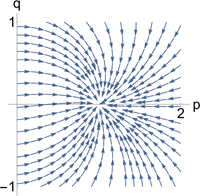
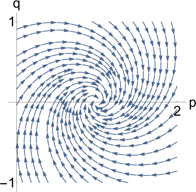
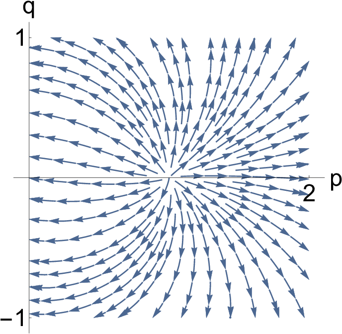
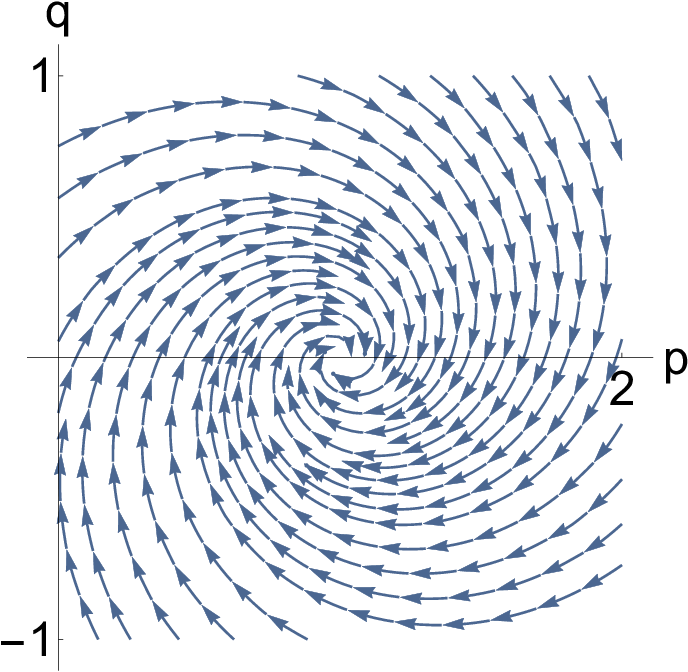
Figure 6: Phase plane streamplots (with Mathematica) in blow-up charts near the equilibrium z−π=(1,0)z_{-}^{\pi}=(1,0) for α=0.5,β=0.1,μ=−1,ccp=0\alpha=0.5\,,\beta=0.1\,,\mu=-1\,,c_{\textnormal{cp}}=0, i.e., the second and third equation of (7). (a-c) θ=0\theta=0 and (d-f) θ=π\theta=\pi. (a,d) codim-2 regime, (b,e) center case, where Ω=β/α+s2/2\Omega=\beta/\alpha+s^{2}/2 holds on the chart θ=π\theta=\pi, and (c,f) codim-0 regime. The remaining parameters and equilibria in (a,d): h=0.5h=0.5, s0=0.12s_{0}=0.12, Ω0=0.44\Omega_{0}=0.44, and z+0=−1.06−0.12​iz_{+}^{0}=-1.06-0.12\mathrm{i}, z+π=−0.94+0.12​iz_{+}^{\pi}=-0.94+0.12\mathrm{i}. In (b,e): h=10.2h=10.2, s0=4s_{0}=4, Ω0=8.2\Omega_{0}=8.2, and z+0=−3−4​iz_{+}^{0}=-3-4\mathrm{i}, z+π=1+4​iz_{+}^{\pi}=1+4\mathrm{i}. In (c,f): h=50.0h=50.0, s0=19.92s_{0}=19.92, Ω0=40.04\Omega_{0}=40.04, and z+0=−10.96−19.92​iz_{+}^{0}=-10.96-19.92\mathrm{i}, z+π=8.96+19.92​iz_{+}^{\pi}=8.96+19.92\mathrm{i}.

Domain walls are heteroclinic orbits between the blow-up charts and decisive for their bifurcation structure are the dimensions (and directions) of un/stable manifolds of the equilibria on these charts. Hence, we next discuss the equilibria Z±0Z^{0}_{\pm} and Z±πZ^{\pi}_{\pm} and their stability.

Transverse to the blow-up charts in θ\theta-direction we readily compute the linearization ∂θ(sin⁡(θ)​p)=cos⁡(θ)​p\partial_{\theta}(\sin(\theta)p)=\cos(\theta)p, i.e., the transverse eigenvalue is −Aθ⋅Re(z±θ)-A^{\theta}\cdot\mathrm{Re}(z^{\theta}_{\pm}) at θ=0\theta=0 and π\pi, respectively. The eigenvalues within the blow-up charts are determined by ±i​γ\pm\mathrm{i}\gamma. With σ=±\sigma=\pm, respectively, the eigenvalues for Zσ0Z^{0}_{\sigma} are

ν1,σ0=−σ​i​γ0,ν2,σ0=ν1,σ0¯,ν3,σ0=Re⁡(zσ0)\nu^{0}_{1,\sigma}=-\sigma\mathrm{i}\gamma^{0}\,,\quad\nu^{0}_{2,\sigma}=\overline{\nu^{0}_{1,\sigma}}\,,\quad\nu^{0}_{3,\sigma}=\mathrm{Re}(z^{0}_{\sigma}) (15)

and for ZσπZ^{\pi}_{\sigma}

ν1,σπ=σ​i​γπ,ν2,σπ=ν1,σπ¯,ν3,σπ=−Re⁡(zσπ).\nu^{\pi}_{1,\sigma}=\sigma\mathrm{i}\gamma^{\pi}\,,\quad\nu^{\pi}_{2,\sigma}=\overline{\nu^{\pi}_{1,\sigma}}\,,\quad\nu^{\pi}_{3,\sigma}=-\mathrm{Re}(z^{\pi}_{\sigma}). (16)

Therefore, the signs of the real parts within each blow-up chart are opposite at Z+πZ^{\pi}_{+} compared to Z−πZ^{\pi}_{-} and determined by the sign of Re⁡(ν1,+0,π)\mathrm{Re}\left(\nu^{0,\pi}_{1,+}\right). Hence, within the blow-up charts each equilibrium is either two-dimensionally stable, unstable or a linearly neutral center point.

For completeness, we next note that the equilibria on both blow-up charts can be neutral centers simultaneously (cf. Figure 3). However, this requires a negative spin polarization and a small Gilbert damping factor, and is not further studied in this paper.

Remark 4.

The equilibria of both blow-up charts are centers simultaneously, if and only if Im⁡(±γ0,π)=0\mathrm{Im}(\pm\gamma^{0,\pi})=0 and γ0,π≠0\gamma^{0,\pi}\neq 0 (compare Lemma 2). For example if α=0.5,β=0.1,μ=−1,ccp=−0.99,h=10\alpha=0.5,\beta=0.1,\mu=-1,c_{\textnormal{cp}}=-0.99,h=10

s2=3960199,Ω=β/α1−ccp+s22=2000199,s^{2}=\frac{3960}{199}\,,\quad\Omega=\frac{\beta/\alpha}{1-c_{\textnormal{cp}}}+\frac{s^{2}}{2}=\frac{2000}{199}\,,

we obtain

γ0=3.33551,γπ=3.27469.\gamma^{0}=3.33551\,,\quad\gamma^{\pi}=3.27469\,.

3 Domain Walls

All domain walls between ±𝒆3\pm\boldsymbol{e}_{3} that we are aware of are of coherent structure type, and thus in one-to-one correspondence to heteroclinic connections between the blow-up charts {θ=0}\{\theta=0\} and {θ=π}\{\theta=\pi\} in (7). Typically we expect these to be heteroclinics between equilibria within the charts, but this is not necessary. Based on the previous analysis, there are three options for heteroclinics between the charts: point-to-point, point-to-cycle, and cycle-to-cycle. We study the first two in this section, for which Proposition 2 implies uniqueness of the DW (up to translations/rotations) for a given set of parameters. The third case can occur at most in a relatively small set of parameters (see Remark 4). Its analysis is beyond the scope of this paper.

Note that in case of an existing connection between an equilibrium and a periodic orbit (see Proposition 1), the domain wall is automatically an inhomogeneous non-flat one. Moreover, via the singular coordinate change any such heteroclinic solution is heteroclinic between θ=0,π\theta=0,\pi in (6) and through the spherical coordinates it is a heteroclinic connection between ±𝒆3\pm\boldsymbol{e}_{3} in the sphere, possibly with unbounded φ\varphi.

3.1 Homogeneous Domain Walls

It is known from [13] in case β=0\beta=0 and from [12] in case ccp=0c_{\textnormal{cp}}=0 (and arbitrary β\beta) that (7) admits for μ<0\mu<0 a family of explicit homogeneous DWs 𝒎0\boldsymbol{m}_{0} given by

(θ0p0q0)=(2​arctan⁡(eσ​−μ​ξ)σ​−μ0)\begin{pmatrix}\theta_{0}\\ p_{0}\\ q_{0}\end{pmatrix}=\begin{pmatrix}2\arctan\left(\mathrm{e}^{\sigma\sqrt{-\mu}\xi}\right)\\ \sigma\sqrt{-\mu}\\ 0\end{pmatrix} (17)

and parameterized by Ω=h+α​β1+α2\Omega=\frac{h+\alpha\beta}{1+\alpha^{2}}, s2=−(β−α​h)2μ​(1+α2)2>0s^{2}=-\frac{(\beta-\alpha h)^{2}}{\mu(1+\alpha^{2})^{2}}>0, and σ=1\sigma=1 for positive speed ss and σ=−1\sigma=-1 for negative ss; the family extends to s=0s=0 in the limit h→βαh\to\frac{\beta}{\alpha} with scaling of the frequency by Ω=βα+−μα​s\Omega=\frac{\beta}{\alpha}+\frac{\sqrt{-\mu}}{\alpha}s. For s=0s=0 (standing) fronts with both orientations exist simultaneously ccp=0c_{\textnormal{cp}}=0 and are given by

(θ0p0q0)=(2​arctan⁡(e±−μ​ξ)±−μ0).\begin{pmatrix}\theta_{0}\\ p_{0}\\ q_{0}\end{pmatrix}=\begin{pmatrix}2\arctan\left(\mathrm{e}^{\pm\sqrt{-\mu}\xi}\right)\\ \pm\sqrt{-\mu}\\ 0\end{pmatrix}.

Hence, the branches of left and right moving walls as parametrized by ss each have termination point at s=0s=0 (cf. Figure 13).

The family of explicit DWs (17) have domain wall width −μ\sqrt{-\mu}, a profile independent of the applied field hh and propagate along a nanowire (μ<0\mu<0) with velocity ss while precessing with azimuthal velocity Ω\Omega. Since these are unique up to spatial reflection symmetry, the direction of motion is related to the spatial direction of connecting ±𝒆3\pm\boldsymbol{e}_{3} through σ\sigma,

θ⁡(−∞)\displaystyle\theta(-\infty) =0\displaystyle=0 θ⁡(+∞)\displaystyle\theta(+\infty) =π\displaystyle=\pi ⇔s\displaystyle\Leftrightarrow s >0​ (wall moves to the right)\displaystyle>0\textnormal{ (wall moves to the right)} (18)
θ⁡(−∞)\displaystyle\theta(-\infty) =π\displaystyle=\pi θ⁡(+∞)\displaystyle\theta(+\infty) =0\displaystyle=0 ⇔s\displaystyle\Leftrightarrow s <0​ (wall moves to the left).\displaystyle<0\textnormal{ (wall moves to the left)}.

To simplify some notation we will focus on the case of right-moving walls including standing walls (s≥0s\geq 0) and thus make the standing assumptions that h≥β/αh\geq\beta/\alpha as well as μ<0\mu<0. We therefore have a 1-to-1 relation of parameters (α,β,h,μ)(\alpha,\beta,h,\mu) and right-moving DWs from

𝒎⁡(ξ,t)=𝒎0​(ξ,t,α,β,h,μ)\boldsymbol{m}(\xi,t)=\boldsymbol{m}_{0}(\xi,t;\alpha,\beta,h,\mu)

with speed and frequency given by

s0=s0​(α,β,h,μ):=α​h−β−μ​(1+α2),Ω0=Ω0​(α,β,h,μ):=h+α​β1+α2s_{0}=s_{0}(\alpha,\beta,h,\mu):=\frac{\alpha h-\beta}{\sqrt{-\mu}(1+\alpha^{2})}\;,\quad\Omega_{0}=\Omega_{0}(\alpha,\beta,h,\mu):=\frac{h+\alpha\beta}{1+\alpha^{2}} (19)

where the subindex 00 emphasizes that ccp=0c_{\textnormal{cp}}=0. Since s0s_{0} is surjective on ℝ≥0\mathbb{R}_{\geq 0} any velocity can be realised. Spatial reflection covers the case h≤β/αh\leq\beta/\alpha.

Based on Lemma 1 as well as Remark 3 for ccp=0c_{\textnormal{cp}}=0 and (homogeneous) speed and frequency (19), one readily finds the asymptotic states of (7) given by

E0≔Z−0|(s0,Ω0)=(0,−μ,0)𝖳andEπ≔Z−π|(s0,Ω0)=(π,−μ,0)𝖳,E^{0}\coloneqq Z^{0}_{-}\big|_{(s_{0},\Omega_{0})}=\left(0,\sqrt{-\mu},0\right)^{\mkern-1.2mu\mathsf{T}}\quad\textnormal{and}\quad E^{\pi}\coloneqq Z^{\pi}_{-}\big|_{(s_{0},\Omega_{0})}=\left(\pi,\sqrt{-\mu},0\right)^{\mkern-1.2mu\mathsf{T}},

with (spatial) eigenvalues (15), (16) given by

νk,−0:=−αs0−2−μ−(−1)kis0,ν03,−=−μ,νk,−π:=−αs0+2−μ−(−1)kis0,νπ3,−=−−μ,\begin{split}\nu_{k,-}^{0}&:=-\alpha s_{0}-2\sqrt{-\mu}-(-1)^{k}\,\mathrm{i}s_{0}\,,\quad\nu^{0}_{3,-}=\sqrt{-\mu}\,,\\ \nu_{k,-}^{\pi}&:=-\alpha s_{0}+2\sqrt{-\mu}-(-1)^{k}\,\mathrm{i}s_{0}\,,\quad\nu^{\pi}_{3,-}=-\sqrt{-\mu}\,,\end{split} (20)

where k=1,2k=1,2. Note that the above equilibria cannot be centers simultaneously (recall μ<0\mu<0), hence a cycle-to-cycle connection can not exist close to it (see Remark 4 for details). For this reason, we focus on point-to-point as well as point-to-cycle connections.

3.2 Inhomogeneous Domain Walls

Homogeneous DWs exist only in case ccp=0c_{\textnormal{cp}}=0 [12, Theorem 5], are explicitly given by (17) and completely characterized by (19). By [12, Theorem 6], fast inhomogeneous DW solutions with |s|≫1|s|\gg 1 exist for any ccp∈(−1,1)c_{\textnormal{cp}}\in(-1,1), but in contrast to (17), the gradient of these profiles is of order 1/|s|1/|s| and thus have a large ‘width’. The natural question arises what happens for any ss in case ccp≠0c_{\textnormal{cp}}\neq 0.

This section contains the main results of this paper: the existence, parameter selection and structure of inhomogeneous DW solutions in case of small |ccp||c_{\textnormal{cp}}| for any value of the applies field hh, and thus any speed ss. This will be achieved by perturbing away from the explicit solution 𝒎0\boldsymbol{m}_{0} given by (17), where the bifurcation structure is largely determined by comparing the dimensions of the un/stable eigenspaces at the asymptotic equilibrium states, which are determined by (20).

Let Ws/u0W^{0}_{s/u} and Ws/uπW^{\pi}_{s/u} denote the stable and unstable manifolds associated to E0E^{0} and EπE^{\pi}, respectively, and ws/u0w_{s/u}^{0} as well as ws/uπw_{s/u}^{\pi} be the dimension of these manifolds so that ws0+wu0=wsπ+wuπ=3w^{0}_{s}+w^{0}_{u}=w^{\pi}_{s}+w^{\pi}_{u}=3. Notably ws0=2w^{0}_{s}=2 and wu0=1w^{0}_{u}=1 for all values of the parameters, and wsπw^{\pi}_{s} is either 11 or 33. Recall the standing assumption s0≥0s_{0}\geq 0.

If wsπ=1w^{\pi}_{s}=1, the heteroclinic connection of E0E^{0} and EπE^{\pi} generically has codimension-2, while for wsπ=3w^{\pi}_{s}=3 it has codimension-0, and we refer to the transition point between these cases, following the discussion in § 2.1.1, as the center case. From (20) we have wsπ=1⇔0≤s0<2​−μαw^{\pi}_{s}=1\Leftrightarrow 0\leq s_{0}<\frac{2\sqrt{-\mu}}{\alpha}, wsπ=3⇔s0>2​−μαw^{\pi}_{s}=3\Leftrightarrow s_{0}>\frac{2\sqrt{-\mu}}{\alpha} and the center case at s0=2​−μαs_{0}=\frac{2\sqrt{-\mu}}{\alpha}.

Hence, within the family of homogeneous DWs given by (17) and satisfying (19), the different bifurcation cases have speed and frequency relations

codim-0: s0>2​−μαandΩ0>βα−2​μα2,\displaystyle s_{0}>\frac{2\sqrt{-\mu}}{\alpha}\quad\textnormal{and}\quad\Omega_{0}>\frac{\beta}{\alpha}-\frac{2\mu}{\alpha^{2}}\,,
center: s0=2​−μαandΩ0=βα−2​μα2,\displaystyle s_{0}=\frac{2\sqrt{-\mu}}{\alpha}\quad\textnormal{and}\quad\Omega_{0}=\frac{\beta}{\alpha}-\frac{2\mu}{\alpha^{2}}\,,
codim-2: 0≤s0<2​−μαandβα≤Ω0<βα−2​μα2.\displaystyle 0\leq s_{0}<\frac{2\sqrt{-\mu}}{\alpha}\quad\textnormal{and}\quad\frac{\beta}{\alpha}\leq\Omega_{0}<\frac{\beta}{\alpha}-\frac{2\mu}{\alpha^{2}}.

Using (19) these can be written in terms of the parameters of (LLGS), which gives the characterization mentioned in the introduction §1.

Remark 5.

The case distinction is also related to the spectral stability of the asymptotic states 𝐦=±𝐞3\boldsymbol{m}=\pm\boldsymbol{e}_{3} in the dynamics of the full PDE (LLGS) which is beyond the scope of this paper, but see Figure 3 for an illustration. In short, it follows from, e.g., [12, Lemma 1] that 𝐞3\boldsymbol{e}_{3} is L2L^{2}-stable for h>β/αh>\beta/\alpha, while −𝐞3-\boldsymbol{e}_{3} is L2L^{2}-stable for h<β/α−μh<\beta/\alpha-\mu and unstable for h>β/α−μh>\beta/\alpha-\mu. Based on this, the stability curves in Figure 3 are defined as follows

Γ+≔β/αh−μ−1,Γ−≔1−β/αh+μ,\Gamma^{+}\coloneqq\frac{\beta/\alpha}{h-\mu}-1,\qquad\Gamma^{-}\coloneqq 1-\frac{\beta/\alpha}{h+\mu},

which intersect at

h=β2​α+β24​α2+μ2.h=\frac{\beta}{2\alpha}+\sqrt{\frac{\beta^{2}}{4\alpha^{2}}+\mu^{2}}.

Since the destabilisation of −𝐞3-\boldsymbol{e}_{3} if β>0\beta>0 corresponds to a Hopf-instability of the ((purely essential)) spectrum, it is effectively invisible in the coherent structure ODE, which detects changes in the linearization at zero temporal eigenvalue only. Visible from the PDE stability viewpoint is a transition of absolute spectrum through the origin in the complex plane of temporal eigenmodes, cf. [18]. Now in the center case, the state −𝐞3-\boldsymbol{e}_{3} is already L2L^{2}-unstable since α>0\alpha>0 as well as μ<0\mu<0 and h>β/αh>\beta/\alpha implies

h=h∗=βα−2​μα2​(1+α2)>βα−μh=h^{\ast}=\frac{\beta}{\alpha}-\frac{2\mu}{\alpha^{2}}(1+\alpha^{2})>\frac{\beta}{\alpha}-\mu

and therefore that Γ−\Gamma^{-} never intersects the line ccp≡0c_{\textnormal{cp}}\equiv 0 at h=h∗h=h^{\ast}.

Moreover, it was shown in [19] that the family of explicit homogeneous DWs (9) is (l​i​n​e​a​r​l​ylinearly) stable for sufficiently small applied fields, actually for h<−μ/2h<-\mu/2, in case β=0\beta=0, hence in the bi-stable case where ±𝐞3\pm\boldsymbol{e}_{3} are L2L^{2}-stable. As mentioned before, β=0\beta=0 is equivalent to ccp=0c_{\textnormal{cp}}=0 in the LLGS equation with an additional shift in hh and β\beta, which leads to the (LLG) case. We expect these DWs are also stable for small perturbations in ccpc_{\textnormal{cp}}, due to the properties of the operator established in [19], but further analysis also on the transition from convective/transient to absolute instability will be done elsewhere.

With these preparations, we next state the main results, which concern existence of DWs in the three regimes.

Theorem 1.

For any parameter set (α0,β0,h0,μ0)(\alpha_{0},\beta_{0},h_{0},\mu_{0}) in the codim-0 case, i.e., μ0<0\mu_{0}<0 and h0>β0/α0−2​μ0−2​μ0/α02h_{0}>\beta_{0}/\alpha_{0}-2\mu_{0}-2\mu_{0}/\alpha_{0}^{2}, the following holds. The explicit homogeneous DWs 𝐦0\boldsymbol{m}_{0} in (9) lies in a smooth family 𝐦ccp\boldsymbol{m}_{c_{\textnormal{cp}}} of DWs parameterized by (ccp,α,β,h,μ,s,Ω)(c_{\textnormal{cp}},\alpha,\beta,h,\mu,s,\Omega) near (0,α0,β0,h0,μ0,s0,Ω0)(0,\alpha_{0},\beta_{0},h_{0},\mu_{0},s_{0},\Omega_{0}) with s0s_{0}, Ω0\Omega_{0} from (19) evaluated at (α0,β0,h0,μ0)(\alpha_{0},\beta_{0},h_{0},\mu_{0}). Moreover, in case ccp=0c_{\textnormal{cp}}=0 and (s,Ω)≠(s0,Ω0)(s,\Omega)\neq(s_{0},\Omega_{0}) evaluated at (α,β,h,μ)(\alpha,\beta,h,\mu), or ccp≠0c_{\textnormal{cp}}\neq 0, these are inhomogeneous flat DWs.

Proof.

As mentioned, in the codim-0 case we have wsπ=3w_{s}^{\pi}=3 and for all parameters wu0=1w_{u}^{0}=1. Due to the existence of the heteroclinic orbit (17), this means Wu0W^{0}_{u} intersects WsπW^{\pi}_{s} transversely and non-trivially for ccp=0c_{\textnormal{cp}}=0 in a unique trajectory. Therefore, this DW perturbs to a locally unique family by the implicit function theorem for perturbations of the parameters in (7).

For ccp≠0c_{\textnormal{cp}}\neq 0 sufficiently small these are inhomogeneous DWs since the derivative of the third equation, the qq-equation, in (7) with respect to ccpc_{\textnormal{cp}} is nonzero in this case; hence already the equilibrium states move into the inhomogeneous regime.

For ccp=0c_{\textnormal{cp}}=0 but (s,Ω)≠(s0,Ω0)(s,\Omega)\neq(s_{0},\Omega_{0}) at (α,β,h,μ)(\alpha,\beta,h,\mu), it follows from [12, Theorem 5] that these DWs cannot be homogeneous. ∎

Next we consider the center case, where h=h∗=β/α−2​μ−2​μ/α2h=h^{\ast}=\beta/\alpha-2\mu-2\mu/\alpha^{2}. We start with a result that follows from the same approach used in the codim-2 case and give refined results below.

Corollary 1.

The statement of Theorem 1 also holds for a parameter set in the center case if the perturbed parameters (ccp,α,β,h,μ,s,Ω)(c_{\textnormal{cp}},\alpha,\beta,h,\mu,s,\Omega) satisfy Ω>s2/2+𝛃−/α\Omega>s^{2}/2+\boldsymbol{\beta}^{-}/\alpha. If Ω=s2/2+𝛃−/α\Omega=s^{2}/2+\boldsymbol{\beta}^{-}/\alpha and Ω<h+μ+s24​(1+α2)\Omega<h+\mu+\frac{s^{2}}{4}(1+\alpha^{2}) the same holds except the DW is possibly non-flat.

Proof.

It follows from Proposition 1 and the discussion before that Ω>s2/2+𝜷−/α\Omega>s^{2}/2+\boldsymbol{\beta}^{-}/\alpha for the parameter perturbation implies that the eigenvalues of the perturbed equilibrium Z−π≈EπZ^{\pi}_{-}\approx E^{\pi} satisfy Re⁡(νk,−π)<0\mathrm{Re}(\nu_{k,-}^{\pi})<0, k=1,2k=1,2. Hence, the stable manifold at the target equilibrium is two-dimensional and lies in a smooth family with the center-stable manifold at the transition point. Then the proof is the same as in the codim-0 case. If the perturbation has Ω=s2/2+𝜷−/α\Omega=s^{2}/2+\boldsymbol{\beta}^{-}/\alpha then we consider as target manifold the three-dimensional stable manifold of a neighborhood of Z−πZ^{\pi}_{-} within the blow-up chart θ=0\theta=0. This neighborhood consists of periodic orbits by Proposition 1 if Ω<h+μ+s24​(1+α2)\Omega<h+\mu+\frac{s^{2}}{4}(1+\alpha^{2}). By dimensionality the intersection with the unstable manifold of Z−0Z^{0}_{-} persists and yields a heteroclinic orbit from the perturbed equilibrium at θ=0\theta=0 to the blow-up chart at θ=π\theta=\pi. Perturbing ccpc_{\textnormal{cp}} away from zero moves the left-asymptotic state into the inhomogeneous regime and thus generates an inhomogeneous DWs. Note from Proposition 1 that the right-asymptotic state is either an equilibrium with q≠0q\neq 0 or a periodic orbit along which q=0q=0 happens at most at two points. ∎

Next we present a refined result in which we show that typical perturbations indeed give non-flat DWs, i.e., heteroclinic connections with right-asymptotic state being a periodic orbit. The existence of flat DWs for ccp≠0c_{\textnormal{cp}}\neq 0 is severely constrained, but not ruled out by this result. Our numerical results, such as those presented in §4, always lead to a selected solution with a periodic asymptotic state.

In addition, attempts to perform numerical continuation (see §4) of flat DWs to ccp≠0c_{\textnormal{cp}}\neq 0 failed. Here we added the constraint H~=0\widetilde{H}=0 and allowed adjustment the parameters hh and ss, but the continuation process did not converge, which confirms numerically the generic selection of a periodic orbit.

As mentioned before, the right asymptotic state is 𝒆3\boldsymbol{e}_{3} in either case in the PDE coordinates; the difference between flat and non-flat lies in the finer details of how the profile approaches 𝒆3\boldsymbol{e}_{3} in term of pp and also qq, which relates to 𝒎\boldsymbol{m} through (2).

Theorem 2.

Consider the smooth family of DWs from Corollary 1 with ccp=0c_{\textnormal{cp}}=0 for parameters satisfying (12) with fixed α>0\alpha>0, β≥0\beta\geq 0, and μ<0\mu<0. Then there is a neighborhood (ccp,s,h)(c_{\textnormal{cp}},s,h) of (0,s0,h∗)(0,s_{0},h^{*}) such that the following holds. Flat DWs occur at most on a surface in the (ccp,s,h)(c_{\textnormal{cp}},s,h)-parameter space and, for β≠0\beta\neq 0, satisfy |h−h0|2+|s−s0|2=𝒪⁡(|ccp|3)|h-h_{0}|^{2}+|s-s_{0}|^{2}=\mathcal{O}(|c_{\textnormal{cp}}|^{3}), more precisely (31) holds, where h0=h∗h_{0}=h^{\ast} and s0=2​−μ/αs_{0}=2\sqrt{-\mu}/\alpha. Otherwise DWs are non-flat, in particular all DWs not equal to 𝐦0\boldsymbol{m}_{0} for ccp=0c_{\textnormal{cp}}=0 or β=0\beta=0 are non-flat.

Due to its more technical nature, the proof of this theorem is deferred to Appendix 6.1.

It remains to consider the codim-2 case.

Theorem 3.

For any parameter set (α0,β0,h0,μ0)(\alpha_{0},\beta_{0},h_{0},\mu_{0}) in the codim-2 case, i.e., μ0<0\mu_{0}<0 and β0/α0≤h0<β0/α0−2​μ0−2​μ0/α02\beta_{0}/\alpha_{0}\leq h_{0}<\beta_{0}/\alpha_{0}-2\mu_{0}-2\mu_{0}/\alpha_{0}^{2}, the following holds. The explicit homogeneous DWs 𝐦0\boldsymbol{m}_{0} in (9) lies in a smooth family of DWs parameterized by (ccp,α,β,h,μ)(c_{\textnormal{cp}},\alpha,\beta,h,\mu) near (0,α0,β0,h0,μ0)(0,\alpha_{0},\beta_{0},h_{0},\mu_{0}). Here the values of (s,Ω)(s,\Omega) are functions of the parameters (ccp,α,β,h,μ)(c_{\textnormal{cp}},\alpha,\beta,h,\mu) and lie in a neighbourhood of (s0,Ω0)(s_{0},\Omega_{0}) from (19). This family is locally unique near 𝐦0\boldsymbol{m}_{0} and for ccp≠0c_{\textnormal{cp}}\neq 0 consists of inhomogeneous flat DWs.

The proof of Theorem 3 is presented in Appendix 6.2 and is based on the Melnikov method for perturbing from 𝒎0\boldsymbol{m}_{0}. As the unperturbed heteroclinic orbit has codimension two, the bifurcation is studied in a three-parametric family with perturbation parameters η≔(ccp,s,Ω)𝖳\eta\coloneqq\left(c_{\textnormal{cp}},s,\Omega\right)^{\mkern-1.2mu\mathsf{T}}, which yields a two-component splitting function M⁡(η)M(\eta) that measures the mutual displacement of the manifolds Wu0W^{0}_{u} and WsπW^{\pi}_{s}.

Due to the fact that Re⁡(νj,−π)<0\mathrm{Re}(\nu^{\pi}_{j,-})<0 also for β=0\beta=0 in the codim-0 regime and the case β=0\beta=0 is included in Theorem 2 as well as Theorem 3, we immediately get the following result.

Corollary 2.

Inhomogeneous flat DWs also exist in the LLG equation (β=0)(\beta=0), which can be flat or non-flat, respectively.

Theorem 3 completes the existence study of DWs. Therefore, for any value of the applied field hh there exists a heteroclinic connection between the blow-up charts with ccp≠0c_{\textnormal{cp}}\neq 0 and q≢0q\not\equiv 0, thus an inhomogeneous (typically flat) DW. Recall that we have focused on right moving DWs, but all results are also valid for left moving walls due to symmetry. Therefore inhomogeneous DWs exist with ccp≠0c_{\textnormal{cp}}\neq 0 for any value of the applied field h∈ℝh\in\mathbb{R}.

4 Numerical Results

Numerical continuation for ordinary differential equations is an established tool for bifurcation analysis in dynamical system. In this section we present continuation results to illustrate the analytical results discussed in § 3. In particular, we will focus on continuation in the parameter ccpc_{\textnormal{cp}} in the range of (−0.5,0.5)(-0.5,0.5) as this perturbs away from the known family 𝒎0\boldsymbol{m}_{0} from (17) (cf. Figure 1(b)) with speed and frequency determined by (19) for a given applied field. Note that we also focus only on right-moving fronts in this section for reasons of clarity. All results were produced by continuation in AUTO-07P and graphics were created with Mathematica as well as MATLAB.

Heteroclinic orbits were detected as solutions to the boundary value problem given by the desingularized system (7) plus a phase condition and boundary conditions at ξ=−L\xi=-L and ξ=L\xi=L taken from the analytic equilibrium states in pp and qq on the blow-up charts (Remark 3). In the codim-2 case, the four required conditions are the p,qp,q values at the charts. In the center case, the three required conditions are: (1,2) the two p,qp,q values at the left chart and (3) the energy difference determined by the function (13). In the codim-0 case, the two required conditions are the pp values at both charts. Moreover, we found L=50L=50 was sufficiently large.

In order to relate to (LLGS), we plot most of the profiles after blowing down to the sphere rather than using the ODE phase space.

Refer to caption
(a)
Refer to caption
(b)
Figure 7: DWs obtained from continuation of 𝒎0\boldsymbol{m}_{0} in system (7) in the codim-2 regime h=0.5h=0.5 (h∗=10.2h^{\ast}=10.2) with initial speed and frequency s0=0.12s_{0}=0.12 as well as Ω0=0.44\Omega_{0}=0.44, and (ccp,s,Ω)=(−0.5,0.11221,0.44077)(c_{\textnormal{cp}},s,\Omega)=(-0.5,0.11221,0.44077). (a) Projection onto the sphere. (b) Zoom-in of corresponding qq-profile (red) and m1m_{1} component (blue).

Following the standing assumption on positive speeds and using ccpc_{\textnormal{cp}} as well as hh as the main parameters, we keep the other parameters fixed with values

α=0.5,β=0.1,μ=−1.\alpha=0.5,\beta=0.1,\mu=-1.

The value of the applied field for the center case, given the fixed parameters, is h∗=10.2h^{\ast}=10.2 (cf. § 3.2), which leads to s0=4.0s_{0}=4.0 as well as Ω0=8.2\Omega_{0}=8.2 (cf. (19)).

4.1 Codim-2 case

The lower boundary for values of the applied field hh lies in the codim-2 regime and is given by h=β/α=0.2h=\beta/\alpha=0.2. As a first numerical example we consider the slightly larger value h=0.5h=0.5. The results upon continuation in the negative as well as positive direction of ccpc_{\textnormal{cp}} are presented in Figures 2(a), 2(c), and 7. The inhomogeneous nature of these solutions (ccp≠0c_{\textnormal{cp}}\neq 0) is reflected in the significantly varying azimuthal angles, also visible in the oscillatory nature of the m1m_{1} component in Figures 2(c) as well as 7b.

The linear part of the splitting function (33) (see Theorem 3), which predicts the direction of parameter variation for the existence of inhomogeneous DWs (ccp≠0c_{\textnormal{cp}}\neq 0) to leading order, reads in this example

M⁡(ccp,s,Ω)=(−0.00147567−0.4992450.245945−0.000577908−0.245945−0.499245)⋅(ccpsΩ),M(c_{\textnormal{cp}},s,\Omega)=\begin{pmatrix}-0.00147567&-0.499245&0.245945\\ -0.000577908&-0.245945&-0.499245\end{pmatrix}\cdot\begin{pmatrix}c_{\textnormal{cp}}\\ s\\ \Omega\end{pmatrix},

so that M=(0,0)𝖳M=(0,0)^{\mkern-1.2mu\mathsf{T}} for (s,Ω)=(−0.00283744⋅ccp,0.000240252⋅ccp)(s,\Omega)=\left(-0.00283744\cdot c_{\textnormal{cp}},0.000240252\cdot c_{\textnormal{cp}}\right). For the parameter values in Figure 7 and 2(a) we obtain, respectively,

M⁡(−0.5,−0.007788,0.000771)=(0.00481558,0.00181945)𝖳,M(-0.5,-0.007788,0.000771)=\left(0.00481558,0.00181945\right)^{\mkern-1.2mu\mathsf{T}},
M⁡(0.5,−0.007973,0.007173)=(0.00648248,−0.00133122)𝖳.M(0.5,-0.007973,0.007173)=\left(0.00648248,-0.00133122\right)^{\mkern-1.2mu\mathsf{T}}.

Note that here the splitting of the (1-dimensional) unstable manifold of the left equilibrium and the (1-dimensional) stable manifold of the right equilibrium differ, i.e., are in opposite directions (signs) in frequency and speed for variations in ccpc_{\textnormal{cp}}.

Refer to caption
(a)
Refer to caption
(b)
Figure 8: DWs obtained from continuation of 𝒎0\boldsymbol{m}_{0} in system (7) projected onto the sphere in the codim-2 regime h=10.1h=10.1 (h∗=10.2h^{\ast}=10.2) with initial speed and frequency s0=3.96s_{0}=3.96 and Ω0=8.12\Omega_{0}=8.12. (a) (ccp,s,Ω)=(−0.5,3.99541,8.05973)(c_{\textnormal{cp}},s,\Omega)=(-0.5,3.99541,8.05973). (b) (ccp,s,Ω)=(0.5,4.08089,8.22402)(c_{\textnormal{cp}},s,\Omega)=(0.5,4.08089,8.22402).

In addition note the decrease in frequency in the m1m_{1} component, and thus also in the m2m_{2} as a result of the increase of the qq component towards zero, cf. Figure 7b. Here, the azimuthal angle decreases since ϕ=∫q\phi=\int q and q<0q<0.

As a further example in the codim-2 regime, we consider h=10.1<10.2=h∗h=10.1<10.2=h^{\ast} near the upper boundary of the codim-2 regime in terms of the applied field hh. The results of the continuation in ccpc_{\textnormal{cp}} are presented in Figure 8. The linear approximation of the splitting in this case is given by M⁡(−0.5,0.03541,−0.06027)=(−0.000175537,−0.00104378)𝖳M(-0.5,0.03541,-0.06027)=\left(-0.000175537,-0.00104378\right)^{\mkern-1.2mu\mathsf{T}} as well as M⁡(0.5,0.12089,0.10402)=(−0.00149519,0.0014975)𝖳M(0.5,0.12089,0.10402)=\left(-0.00149519,0.0014975\right)^{\mkern-1.2mu\mathsf{T}} in (a) and (b), respectively. Note that the direction of splitting of the two components in this case is also dependent on the polarity sign, as in the previous example. In both cases (h=0.5h=0.5 and h=10.1h=10.1), the continuation results look basically the same in the codim-2 regime, where the solution is, roughly speaking, constantly spiraling down from the north to the south pole.

4.2 Center case

Refer to caption
(a)
Refer to caption
(b)
Figure 9: DWs obtained from continuation of 𝒎0\boldsymbol{m}_{0} in system (7) in the center regime h=h∗=10.2h=h^{\ast}=10.2 with s=s0=4,Ω=Ω0=8.2s=s_{0}=4,\Omega=\Omega_{0}=8.2, and ccp=0.5c_{\textnormal{cp}}=0.5. (a) Projection onto the sphere. (b) Profile of corresponding qq-component.

We perform computations in the center case with applied field h=h∗=10.2h=h^{\ast}=10.2 and fixed frequency Ω=𝜷−/α+s2/2\Omega=\boldsymbol{\beta}^{-}/\alpha+s^{2}/2 (see Proposition 1 and its discussion details). Theorem 2 shows that the right asymptotic state is generically a periodic orbit and more precisely that in case ccp=0c_{\textnormal{cp}}=0, no constellation of hh and ss exists, both not equal to zero, for which the right asymptotic state is the (shifted) equilibrium. The results of continuation in ccpc_{\textnormal{cp}} projected on the sphere look quite the same, which is why only the result for ccp=0.5c_{\textnormal{cp}}=0.5 is presented in Figure 9. The fact that the right asymptotic state is a periodic orbit on the blow-up chart θ=π\theta=\pi is reflected by the nearly constant oscillations in the qq-profile for ξ\xi close to the right boundary (cf. Figure 9b).

Refer to caption
(a)
Refer to caption
(b)
Refer to caption
(c)
Figure 10: Continuation of 𝒎0\boldsymbol{m}_{0} in system (7) in the center case with applied field h=h∗=10.2h=h^{\ast}=10.2 and fixed frequency Ω=𝜷−/α+s2/2\Omega=\boldsymbol{\beta}^{-}/\alpha+s^{2}/2; here s0=4s_{0}=4. Shown is the energy difference (solid blue line) between the equilibrium and asymptotic state from continuation on right boundary against the continuation parameter ccpc_{\textnormal{cp}} in (a), hh in (b), and ss in (c). The red dashed curve in (b) and (c) is the quadratic approximation (21).

That the right state is not the equilibrium in the blow-up chart is further corroborated by computing the difference in energy H~\widetilde{H} between this equilibrium state (see Remark 3) and the approximate right asymptotic state obtained from continuation. The analytic prediction of this difference up to second order is given by (31), which reads, for the chosen parameters,

−0.006612+0.00673​s−0.00183​s2−0.00134​h−0.000086​h2+0.00077​h​s.-0.006612+0.00673s-0.00183s^{2}-0.00134h-0.000086h^{2}+0.00077hs\,. (21)

As this analytic prediction is independent of ccpc_{\textnormal{cp}} the dependence of H~\widetilde{H} on ccp≈0c_{\textnormal{cp}}\approx 0 is of cubic or higher power. Indeed, the results plotted in Figure 10a suggest an at least quartic dependence since a maximum lies at ccp=0c_{\textnormal{cp}}=0. The asymmetric nature of the graph suggests that odd powers appear in the expansion beyond our analysis, but also note the order of ​10−6{10}^{-6} in H~\widetilde{H}. In addition to the dependence on ccpc_{\textnormal{cp}}, continuations for ccp=0c_{\textnormal{cp}}=0 of H~\widetilde{H} in hh with fixed s=s0=4s=s_{0}=4 and in ss with fixed h=h∗=10.2h=h^{\ast}=10.2 are plotted in Figure 10b and 10c, respectively. Here we also plot the quadratic prediction (21).

4.3 Codim-0 case

Next, we consider an applied field h=10.3h=10.3 in the codim-0 regime, just above the applied field value for the center case h∗=10.2h^{*}=10.2. The results of continuation in ccpc_{\textnormal{cp}} are plotted on the sphere in Figure 11. The azimuthal profile in ϕ\phi and hence in qq are non-trivial as predicted for inhomogeneous DWs.

In the ODE, qq possesses an oscillating profile and has a monotonically decreasing amplitude in both cases. This is a consequence of the proximity to the center case and the convergence to equilibria (see § 3.2 for details). Recall that the speed and frequency are not selected by the existence problem during continuation in ccpc_{\textnormal{cp}}, but are taken as the fixed parameters (s0,Ω0)(s_{0},\Omega_{0}) defined in (19).

Refer to caption
(a)
Refer to caption
(b)
Figure 11: DWs obtained from continuation of 𝒎0\boldsymbol{m}_{0} in system (7) projected onto the sphere in the codim-0 regime h=10.3h=10.3 (h∗=10.2h^{\ast}=10.2) and initial speed and frequency s0=4.04s_{0}=4.04 and Ω0=8.28\Omega_{0}=8.28. (a) ccp=−0.5c_{\textnormal{cp}}=-0.5. (b) ccp=0.5c_{\textnormal{cp}}=0.5.

The final example is for a relatively large applied field h=50h=50 in the codim-0 regime, far away from the center case, and the results of continuation in ccpc_{\textnormal{cp}} projected on the sphere are presented in Figure 2(b) as well as Figure 12a. Moreover, the corresponding m1m_{1} and m2m_{2} profiles for ccp=0.5c_{\textnormal{cp}}=0.5 are presented in Figure 2(d), and for ccp=−0.5c_{\textnormal{cp}}=-0.5, in Figure 12b. As in the previous example, the inhomogeneous nature is visible in the non-trivial azimuthal profile.

Refer to caption
(a)
Refer to caption
(b)
Figure 12: DWs obtained from continuation of 𝒎0\boldsymbol{m}_{0} in system (7) in the codim-0 regime h=50h=50 (h∗=10.2h^{\ast}=10.2) with initial speed and frequency s0=19.92,Ω0=40.04s_{0}=19.92,\Omega_{0}=40.04, and ccp=−0.5c_{\textnormal{cp}}=-0.5. (a) Projection onto the sphere. (b) Zoom-in of the corresponding m1m_{1} (solid blue) and m2m_{2} (dashed red) component.

In summary, switching on the parameter ccpc_{\textnormal{cp}} leads to a variety of inhomogeneous flat as well as non-flat DW solutions, but also in case ccp=0c_{\textnormal{cp}}=0 there exist inhomogeneous DWs (cf. Figure 4) which are much more complex than the homogeneous one given by (9) (cf. Figure 1(b)).

Finally, recall from § 3.1 that in the explicit family (9), the right moving DWs terminate at s=0s=0. The question arises what happens for ccp≠0c_{\textnormal{cp}}\neq 0 along the parameter ss. To study this, we performed a continuation in the parameter ss for different values of ccpc_{\textnormal{cp}}. For decreasing ss we found that numerical continuation failed at some s>0s>0 for ccp≠0c_{\textnormal{cp}}\neq 0 (cf. Figure 13). The details of this apparent existence boundary are beyond the scope of this paper. Note that the special role of ss is reflected in the splitting function (34). In case s0=s=0s_{0}=s=0, the first column of (32) is zero (see (34)) and thus the parameterization of ccpc_{\textnormal{cp}} can not be written as a function in ss.

In detail, we continued the analytic solution (9) in ccpc_{\textnormal{cp}} away from zero for different initial values of β/α<h<h∗\beta/\alpha<h<h^{\ast}. This led to inhomogeneous (ccp≠0c_{\textnormal{cp}}\neq 0) DWs, which we in turn continued in the parameter ss towards zero for different fixed values of ccpc_{\textnormal{cp}} until the continuation process fails to converge. Based on this, there is numerical evidence that DWs with opposite speed sign (counter-propagating fronts) can only exist simultaneously for s=0s=0 (standing fronts). We took a polynomial fit on these points as an approximation of the existence boundary (cf. blue curve in Figure 13a). The continuation process towards the boundary is indicated by red arrows in Figure 13a for positive ccpc_{\textnormal{cp}}. Additionally, the corresponding results in the parameter space Ω\Omega and ccpc_{\textnormal{cp}} is presented in 13b.

Refer to caption
(a)
Refer to caption
(b)
Figure 13: Continuation results in ss and Ω\Omega for fixed ccpc_{\textnormal{cp}} in the codim-2 parameter regime. Further parameters are α=0.5,β=0.1,μ=−1\alpha=0.5,\beta=0.1,\mu=-1, and hh free. Blue solid line represents interpolated termination boundary for ss in (a) and Ω\Omega in (b), respectively. Red arrows indicate continuation approach towards boundary.

As a last point, we briefly describe the numerical method for time-integration near DWs, including freezing of speed and frequency (cf. Figure 4). All calculations were done with the (free) software package pde2path which is based on a Finite Element Method (FEM), cf. [20] and the references therein. Time-integration in pde2path with the so-called ‘freezing’ method is discussed in [21]. In addition to the phase condition for the speed we added a phase condition for the rotation and time-integrated via a semi-implicit Euler scheme.

5 Discussion and Outlook

We have presented results pertaining the existence of different types of domain walls for the LLG as well as LLGS equation. Our main focus has been on a nonzero polarisation parameter ccp≠0c_{\textnormal{cp}}\neq 0 for any value of the applied field, including the high-field case, and thus for any domain wall speed. These results extend what is known in particular for inhomogeneously structured DWs, and we have discovered an apparently new type of DWs with certain oscillatory tails, referred to as non-flat here.

In detail, we have provided a classification of DWs based on co-dimension properties in a reduced (spatial) coherent structure ODE, which relates to stability and selection properties that we review next. First, we have proven the existence of inhomogeneous flat DWs in case ccp=0c_{\textnormal{cp}}=0 as well as ccp≠0c_{\textnormal{cp}}\neq 0 for an applied field above a certain threshold, which is mainly material depending. To our knowledge, the only previous existence result for ccp≠0c_{\textnormal{cp}}\neq 0 with ’large’ applied fields concerns less relevant non-localized DWs [12]. Here the existence problem does not select speed and frequency.

Second, we have discussed the so-called center case, which is characterized by non-hyperbolic equilibria in the underlying coherent structure ODE. In this case, we have shown the existence of inhomogeneous DWs including the leading order selection mechanism. These solutions are non-flat in case ccp=0c_{\textnormal{cp}}=0 and generically also non-flat for ccpc_{\textnormal{cp}} away from zero, which was substantiated by numerical results. The fundamental observation has been the existence of a Hamiltonian function in a certain parameter regime in the corresponding coherent structure ODE.

Third, we have proven the existence of inhomogeneous DWs in the so-called codim-2 regime, which is a range of values for the applied field in which the speed ss is between zero and the center case speed. In this regime, each solution in case ccp≠0c_{\textnormal{cp}}\neq 0 is uniquely determined by its speed as well as frequency. Here we have also presented the leading order selection function in the coherent structure ODE variables pp and qq, which depends on the speed ss, the frequency Ω\Omega, and is independent of ccpc_{\textnormal{cp}} for standing fronts.

We believe that these results are not only interesting and relevant from a theoretical and mathematical viewpoint, but also from an application viewpoint. They could help to better understand the interfaces between different magnetic domains in nanostructures, e.g. in the development of racetrack memories, which are a promising prospective high density storage unit that utilize a series of DWs by shifting at high speed along magnetic nanowires through nanosecond current pulses.

In order to illustrate and corroborate these theoretical results, we have presented numerical computations for a variety of values for the applied field in § 4. On the one hand, the examples in essence show that large applied fields lead to more complex profiles of the DWs in case ccp≠0c_{\textnormal{cp}}\neq 0. On the other hand, while in the center case the DWs projected on the sphere appear similar to those for small applied fields, these solutions approach the poles in a qualitatively different ‘non-flat’ manner – as predicted by our analysis. Moreover, we compared the numerical and analytical results of the selection mechanism in the center case, showing that the analytical leading order approximation predicts the effect of small perturbations in the parameters. Notably, for applied fields above a certain threshold, where the existence analysis does not provide a selection of speed and frequency, numerically the DWs selected in the PDE dynamics are in the center case, both for ccp=0c_{\textnormal{cp}}=0 as well as ccp≠0c_{\textnormal{cp}}\neq 0. Hence, it might be possible to detect these solutions in a high-field regime in real materials.

One question concerning existence beyond our analysis is whether inhomogeneous (flat or non-flat) solutions exist for any value of ccp∈(−1,1)c_{\textnormal{cp}}\in(-1,1), and whether this class could be utilized in applications.

A natural step towards the understanding of domain wall motion in nanowires beyond the question of existence concerns the dynamic stability. For inhomogeneous solutions there appears to be no rigorous result in this direction. In particular for larger applied fields, stability results would be an essential step towards understanding the selection mechanism of solutions in terms of speed and frequency; our first numerical investigations show that solutions in the center parameter regime are selected, i.e., inhomogeneous non-flat DWs.

Moreover, preliminary analytic results, for ccp=0c_{\textnormal{cp}}=0 as well as ccp≠0c_{\textnormal{cp}}\neq 0, show that selection mechanism is mainly determined by the value of the applied field, where in the bi-stable case (±𝒆3\pm\boldsymbol{e}_{3} linearly stable) homogeneous DWs are selected, and in the mono-stable case inhomogeneous non-flat DWs are selected, which will be studied in detail in an upcoming work.

References

  • [1] Stuart SP Parkin, Masamitsu Hayashi, and Luc Thomas. Magnetic domain-wall racetrack memory. Science, 320(5873):190–194, 2008.
  • [2] William Reohr, Heinz Honigschmid, Raphael Robertazzi, Dietmar Gogl, Frank Pesavento, Stefan Lammers, Kelvin Lewis, Christian Arndt, Yu Lu, Hans Viehmann, et al. Memories of tomorrow. IEEE circuits and devices magazine, 18(5):17–27, 2002.
  • [3] CJ Lin, SH Kang, YJ Wang, K Lee, X Zhu, WC Chen, X Li, WN Hsu, YC Kao, MT Liu, et al. 45nm low power cmos logic compatible embedded stt mram utilizing a reverse-connection 1t/1mtj cell. In Electron Devices Meeting (IEDM), 2009 IEEE International, pages 1–4. IEEE, 2009.
  • [4] Moinuddin K Qureshi, Vijayalakshmi Srinivasan, and Jude A Rivers. Scalable high performance main memory system using phase-change memory technology. ACM SIGARCH Computer Architecture News, 37(3):24–33, 2009.
  • [5] Isaak D Mayergoyz, Giorgio Bertotti, and Claudio Serpico. Nonlinear magnetization dynamics in nanosystems. Elsevier, 2009.
  • [6] Alex Hubert and Rudolf Schäfer. Magnetic domains: the analysis of magnetic microstructures. Springer Science & Business Media, 2008.
  • [7] Giorgio Bertotti. Spin-transfer-driven magnetization dynamics. Magnetic Nanostructures in Modern Technology, pages 37–60, 2008.
  • [8] L Berger. Emission of spin waves by a magnetic multilayer traversed by a current. Physical Review B, 54(13):9353, 1996.
  • [9] John C Slonczewski. Current-driven excitation of magnetic multilayers. Journal of Magnetism and Magnetic Materials, 159(1-2):L1–L7, 1996.
  • [10] JA Osborn. Demagnetizing factors of the general ellipsoid. Physical review, 67(11-12):351, 1945.
  • [11] JC Slonczewski. Currents and torques in metallic magnetic multilayers. Journal of Magnetism and Magnetic Materials, 247(3):324–338, 2002.
  • [12] Christof Melcher and Jens DM Rademacher. Pattern formation in axially symmetric landau–lifshitz–gilbert–slonczewski equations. Journal of Nonlinear Science, 27(5):1551–1587, 2017.
  • [13] Arseni Goussev, JM Robbins, and Valeriy Slastikov. Domain-wall motion in ferromagnetic nanowires driven by arbitrary time-dependent fields: An exact result. Physical review letters, 104(14):147202, 2010.
  • [14] Johan Åkerman. Toward a universal memory. Science, 308(5721):508–510, 2005.
  • [15] LD Landau and EM Lifshitz. On the theory of the dispersion of magnetic permeability in ferromagnetic bodies, phy. z. sowjetunion 8: 153. Reproduced in Collected Papers of LD Landau, pages 101–114, 1935.
  • [16] Thomas L Gilbert. A phenomenological theory of damping in ferromagnetic materials. IEEE Transactions on Magnetics, 40(6):3443–3449, 2004.
  • [17] M Lakshmanan. The fascinating world of the landau–lifshitz–gilbert equation: an overview. Philosophical Transactions of the Royal Society of London A: Mathematical, Physical and Engineering Sciences, 369(1939):1280–1300, 2011.
  • [18] Björn Sandstede and Arnd Scheel. Absolute and convective instabilities of waves on unbounded and large bounded domains. Physica D: Nonlinear Phenomena, 145(3-4):233–277, 2000.
  • [19] Yan Gou, Arseni Goussev, JM Robbins, and Valeriy Slastikov. Stability of precessing domain walls in ferromagnetic nanowires. Physical Review B, 84(10):104445, 2011.
  • [20] T Dohnal, J Rademacher, H Uecker, and D Wetzel. pde2path 2.0. ENOC, 2014.
  • [21] Jens DM Rademacher and Hannes Uecker. Symmetries, freezing, and hopf bifurcations of traveling waves in pde2path, 2017.
  • [22] Yuri A Kuznetsov. Elements of applied bifurcation theory, volume 112. Springer Science & Business Media, 2013.

6 Appendix

6.1 Proof of Theorem 2

We use the notation

u=u⁡(ξ,η,α,β,μ)=(θ⁡(ξ,η,α,β,μ),p⁡(ξ,η,α,β,μ),q⁡(ξ,η,α,β,μ))𝖳u=u(\xi;\eta,\alpha,\beta,\mu)=\left(\theta(\xi;\eta,\alpha,\beta,\mu),p(\xi;\eta,\alpha,\beta,\mu),q(\xi;\eta,\alpha,\beta,\mu)\right)^{\mkern-1.2mu\mathsf{T}}

and bifurcation parameters η=(ccp,s,h)𝖳\eta=\left(c_{\textnormal{cp}},s,h\right)^{\mkern-1.2mu\mathsf{T}}, where s0s_{0} and h0=h∗h_{0}=h^{\ast} are defined below (see § 3.2 for details). The starting point for our perturbation analysis are the unperturbed parameters and explicit heteroclinic solution in the center case (12), where the frequency is Ω0=s02/2+β/α\Omega_{0}=s_{0}^{2}/2+\beta/\alpha. These are given by

η0:=(ccp0s0h0):=(02​−μαβα−2​μ−2​μα2)\eta_{0}:=\begin{pmatrix}c_{\textnormal{cp}_{0}}\\ s_{0}\\ h_{0}\end{pmatrix}:=\begin{pmatrix}0\\ \frac{2\sqrt{-\mu}}{\alpha}\\ \frac{\beta}{\alpha}-2\mu-\frac{2\mu}{\alpha^{2}}\end{pmatrix}

as well as

u0=u0​(ξ,η0,α,β,μ):=(θ0​(ξ,η0,α,β,μ)p0​(ξ,η0,α,β,μ)q0​(ξ,η0,α,β,μ)):=(2​arctan⁡(exp⁡(−μ​ξ))−μ0).u_{0}=u_{0}(\xi;\eta_{0},\alpha,\beta,\mu):=\begin{pmatrix}\theta_{0}(\xi;\eta_{0},\alpha,\beta,\mu)\\ p_{0}(\xi;\eta_{0},\alpha,\beta,\mu)\\ q_{0}(\xi;\eta_{0},\alpha,\beta,\mu)\end{pmatrix}:=\begin{pmatrix}2\arctan\left(\exp(\sqrt{-\mu}\;\xi)\right)\\ \sqrt{-\mu}\\ 0\end{pmatrix}.

Unless stated otherwise, we suppress the explicit dependence of uu on α,β\alpha,\beta, and μ\mu in the following discussion. Let us write Zπ:=Z−πZ^{\pi}:=Z^{\pi}_{-} with the notation from Remark 3 so that the unperturbed right asymptotic state is given by

Zπ​(η0)=(π,α​s02,s02−−μα2)𝖳=(π,−μ,0)𝖳Z^{\pi}(\eta_{0})=\left(\pi,\frac{\alpha s_{0}}{2},\frac{s_{0}}{2}-\sqrt{-\frac{\mu}{\alpha^{2}}}\right)^{\mkern-1.2mu\mathsf{T}}=\left(\pi,\sqrt{-\mu},0\right)^{\mkern-1.2mu\mathsf{T}}

and its derivative with respect to η\eta is given by

Zηπ​(η0)=(0000α20β2​−μ2+α22−α2​−μ).Z^{\pi}_{\eta}(\eta_{0})=\begin{pmatrix}0&0&0\\ 0&\frac{\alpha}{2}&0\\ \frac{\beta}{2\sqrt{-\mu}}&\frac{2+\alpha^{2}}{2}&-\frac{\alpha}{2\sqrt{-\mu}}\end{pmatrix}.

We write system (7) for brevity as

u′=f⁡(u,η),u^{\prime}=f(u;\eta)\,, (22)

so f⁡(u,η)f(u;\eta) denotes the right side of (7). The linearization w.r.t. η\eta in the unperturbed heteroclinic connection u0u_{0}, given by (17), is the non-autonomous linear equation

uη′=fu​(u0,η0)​uη+fη​(u0,η0)​η,u_{\eta}^{\prime}=f_{u}(u_{0};\eta_{0})u_{\eta}+f_{\eta}(u_{0};\eta_{0})\eta, (23)

where uη=(θη,pη,qη)𝖳u_{\eta}=\left(\theta_{\eta},p_{\eta},q_{\eta}\right)^{\mkern-1.2mu\mathsf{T}}. Its homogeneous part is

θη′=−μ​cos⁡(θ0)​θη+pη​sin⁡(θ0)pη′=−(α​s0+2​−μ​cos⁡(θ0))​pη+s0​qηqη′=−s0​pη−(α​s0+2​−μ​cos⁡(θ0))​qη,\begin{array}[]{rl}\theta^{\prime}_{\eta}&=\sqrt{-\mu}\cos(\theta_{0})\theta_{\eta}+p_{\eta}\sin(\theta_{0})\\ p^{\prime}_{\eta}&=-\left(\alpha s_{0}+2\sqrt{-\mu}\cos(\theta_{0})\right)p_{\eta}+s_{0}q_{\eta}\\ q^{\prime}_{\eta}&=-s_{0}p_{\eta}-\left(\alpha s_{0}+2\sqrt{-\mu}\cos(\theta_{0})\right)q_{\eta}\end{array}, (24)

with θ0​(ξ)=2​arctan⁡(exp⁡(−μ​ξ))\theta_{0}(\xi)=2\arctan\left(\exp(\sqrt{-\mu}\,\xi)\right) due to (17). We next solve (24) and determine its fundamental solution matrix.

The first obvious vector-solution of it is U1=u0′=(θ0′,0,0)U_{1}=u_{0}^{\prime}=(\theta^{\prime}_{0},0,0) since the second and the third equation of (24) do not depend on θη\theta_{\eta}. The other solutions can be obtained from U1U_{1} and the result of Lemma 1. Changing to polar coordinates

pη=r​cos⁡φ,qη=r​sin⁡φ,p_{\eta}=r\cos\varphi\,,\quad q_{\eta}=r\sin\varphi\,,

the equations for pηp_{\eta} and qηq_{\eta} become

r′=−(α​s0+2​−μ​cos⁡(θ0))​rφ′=−s0,\begin{array}[]{rl}r^{\prime}&=-\left(\alpha s_{0}+2\sqrt{-\mu}\cos(\theta_{0})\right)r\\ \varphi^{\prime}&=-s_{0}\,,\end{array}

whose general solution can be written as

pη=r0​r​(ξ)​cos⁡(−s0​ξ+φ0)qη=r0​r​(ξ)​sin⁡(−s0​ξ+φ0)\begin{array}[]{rl}p_{\eta}&=r_{0}r(\xi)\cos(-s_{0}\xi+\varphi_{0})\\ q_{\eta}&=r_{0}r(\xi)\sin(-s_{0}\xi+\varphi_{0})\end{array}

where

r⁡(ξ)=exp⁡(−α​s0​ξ−2​−μ​∫ξcos⁡(θ0​(τ))​𝑑τ)=(1+e2​−μ​ξ)2​e(−2​−μ−α​s0)​ξ,r(\xi)=\exp\left(-\alpha s_{0}\xi-2\sqrt{-\mu}\int\limits_{\xi}\cos(\theta_{0}(\tau))d\tau\right)=\left(1+\mathrm{e}^{2\sqrt{-\mu}\xi}\right)^{2}\,\mathrm{e}^{(-2\sqrt{-\mu}-\alpha s_{0})\xi},

and r0,φ0r_{0},\varphi_{0} are arbitrary integration constants corresponding to suitable initial conditions. Note that limξ→±∞r⁡(ξ)=∞\lim\limits_{\xi\to\pm\infty}r(\xi)=\infty for 0≤s0<2​−μ/α0\leq s_{0}<2\sqrt{-\mu}/\alpha.

Next, the values of the integration constants have to be selected in order for the second and the third vector-solutions

U2=(θ11r1​r​(ξ)​cos⁡(−s0​ξ+φ1)r1​r​(ξ)​sin⁡(−s0​ξ+φ1)),U3=(θ12r2​r​(ξ)​cos⁡(−s0​ξ+φ2)r2​r​(ξ)​sin⁡(−s0​ξ+φ2))U_{2}=\begin{pmatrix}\theta^{1}_{1}\\ r_{1}r(\xi)\cos(-s_{0}\xi+\varphi_{1})\\ r_{1}r(\xi)\sin(-s_{0}\xi+\varphi_{1})\end{pmatrix}\,,\quad U_{3}=\begin{pmatrix}\theta^{2}_{1}\\ r_{2}r(\xi)\cos(-s_{0}\xi+\varphi_{2})\\ r_{2}r(\xi)\sin(-s_{0}\xi+\varphi_{2})\end{pmatrix} (25)

to be linearly independent. Here θ11,θ12\theta^{1}_{1},\theta^{2}_{1} are not relevant for what follows. The determinant of the fundamental matrix reads

detΦ⁡(ξ)=det(U1​(ξ),U2​(ξ),U3​(ξ))=r1​r2​r2​(ξ)​θ0′​(ξ)​sin⁡(φ2−φ1),\det\Phi(\xi)=\det\left(U_{1}(\xi),U_{2}(\xi),U_{3}(\xi)\right)=r_{1}r_{2}r^{2}(\xi)\theta^{\prime}_{0}(\xi)\sin(\varphi_{2}-\varphi_{1}),

which is non-zero for r1=r2=1r_{1}=r_{2}=1, φ1=0\varphi_{1}=0 and φ2=π/2\varphi_{2}=\pi/2, i.e. detΦ⁡(ξ)=r2​(ξ)​θ0′​(ξ)\det\Phi(\xi)=r^{2}(\xi)\theta^{\prime}_{0}(\xi). Together, we get the fundamental solution matrix of the homogeneous part as

Φ⁡(ξ)=(θ0′​(ξ)θ11​(ξ)θ12​(ξ)0r⁡(ξ)​cos⁡(−s0​ξ)−r⁡(ξ)​sin⁡(−s0​ξ)0r⁡(ξ)​sin⁡(−s0​ξ)r⁡(ξ)​cos⁡(−s0​ξ)).\Phi(\xi)=\begin{pmatrix}\theta^{\prime}_{0}(\xi)&\theta^{1}_{1}(\xi)&\theta^{2}_{1}(\xi)\\ 0&r(\xi)\cos(-s_{0}\xi)&-r(\xi)\sin(-s_{0}\xi)\\ 0&r(\xi)\sin(-s_{0}\xi)&r(\xi)\cos(-s_{0}\xi)\end{pmatrix}. (26)

The derivative of (22) with respect to η\eta is given by (23) and from the variation of constants formula we get for some ξ0\xi_{0} that

uη​(ξ)=Φξ,ξ0​uη​(ξ0)+∫ξ0ξΦξ,τ​fη​(u0​(τ),η0)​𝑑τ,u_{\eta}(\xi)=\Phi_{\xi,\xi_{0}}u_{\eta}(\xi_{0})+\int\limits_{\xi_{0}}^{\xi}{\Phi_{\xi,\tau}f_{\eta}(u_{0}(\tau);\eta_{0})d\tau}\,,

where Φξ,τ=Φ⁡(ξ)⋅Φ−1​(τ)\Phi_{\xi,\tau}=\Phi(\xi)\cdot\Phi^{-1}(\tau) is the evolution operator. Using (26) we find

Φξ,τ​(ξ,τ,η)=(Θ1Θ2Θ30r⁡(ξ)r⁡(τ)​cos⁡(−s0​(ξ−τ))−r⁡(ξ)r⁡(τ)​sin⁡(−s0​(ξ−τ))0r⁡(ξ)r⁡(τ)​sin⁡(−s0​(ξ−τ))r⁡(ξ)r⁡(τ)​cos⁡(−s0​(ξ−τ))),\Phi_{\xi,\tau}(\xi,\tau;\eta)=\begin{pmatrix}\Theta_{1}&\Theta_{2}&\Theta_{3}\\ 0&\frac{r(\xi)}{r(\tau)}\cos\left(-s_{0}(\xi-\tau)\right)&-\frac{r(\xi)}{r(\tau)}\sin\left(-s_{0}(\xi-\tau)\right)\\ 0&\frac{r(\xi)}{r(\tau)}\sin\left(-s_{0}(\xi-\tau)\right)&\frac{r(\xi)}{r(\tau)}\cos\left(-s_{0}(\xi-\tau)\right)\end{pmatrix}, (27)

where the explicit forms of the functions Θ1,2,3​(ξ)\Theta_{1,2,3}(\xi) are not relevant for the remainder of this proof. Since uη​(ξ)u_{\eta}(\xi) tends to ∂ηZ−0\partial_{\eta}Z^{0}_{-} for ξ→−∞\xi\to-\infty the hyperbolicity of Z−0Z^{0}_{-} (more precisely the resulting exponential dichotomy) implies Φξ,ξ0​uη​(ξ0)→0\Phi_{\xi,\xi_{0}}u_{\eta}(\xi_{0})\to 0 as ξ0→−∞\xi_{0}\to-\infty and so

uη​(ξ)=∫−∞ξΦξ,τ​fη​(u⁡(τ,η0),η0)​𝑑τ.u_{\eta}(\xi)=\int\limits_{-\infty}^{\xi}{\Phi_{\xi,\tau}f_{\eta}(u(\tau;\eta_{0});\eta_{0})d\tau}\,. (28)

Regarding the limiting behavior as ξ→∞\xi\to\infty, recall that Corollary 1 states that the right asymptotic limit of the perturbed heteroclinic orbit is either the perturbed equilibrium Zπ​(η)Z^{\pi}(\eta) or a periodic orbit around it in the blow-up chart at θ=π\theta=\pi. The integral (28) distinguishes these case in the sense that either it has a limit as ξ→+∞\xi\to+\infty so the heteroclinic orbit connects the two equilibria, or it does not and the heteroclinic orbit connects to a periodic solution.

We next determine uη​(ξ)u_{\eta}(\xi) componentwise

uη​(ξ)=v≔(v11v12v13v21v22v23v31v32v33),u_{\eta}(\xi)=v\coloneqq\begin{pmatrix}v_{11}&v_{12}&v_{13}\\ v_{21}&v_{22}&v_{23}\\ v_{31}&v_{32}&v_{33}\end{pmatrix},

where vi​jv_{ij} are the components of (28) and index i=1,2,3i=1,2,3 relates to θ,p,q\theta,p,q as well as j=1,2,3j=1,2,3 to ccp,s,hc_{\textnormal{cp}},s,h.

Towards this, we compute

fη​(u0​(τ),η0)=(000−β/α−−μα​(2+α2)12​β1+e2​−μ​τ−μ0),f_{\eta}(u_{0}(\tau),\eta_{0})=\begin{pmatrix}0&0&0\\ -\beta/\alpha&-\frac{\sqrt{-\mu}}{\alpha}(2+\alpha^{2})&1\\ \frac{2\beta}{1+\mathrm{e}^{2\sqrt{-\mu}\;\tau}}&\sqrt{-\mu}&0\end{pmatrix},

and together with (28) and (27) we obtain

v21=−βα​IC−2​β​JS,v_{21}=-\frac{\beta}{\alpha}I_{C}-2\beta J_{S}\,, v22=−−μα​(2+α2)​IC−−μ​IS,v_{22}=-\frac{\sqrt{-\mu}}{\alpha}(2+\alpha^{2})I_{C}-\sqrt{-\mu}I_{S}\,, v23=IC,v_{23}=I_{C}\,,
v31=−βα​IS+2​β​JC,v_{31}=-\frac{\beta}{\alpha}I_{S}+2\beta J_{C}\,, v32=−−μα​(2+α2)​IS+−μ​ICv_{32}=-\frac{\sqrt{-\mu}}{\alpha}(2+\alpha^{2})I_{S}+\sqrt{-\mu}I_{C} v33=IS,v_{33}=I_{S}\,,

where

IC=IC​(ξ)≔∫−∞ξ(1+exp⁡(−2​−μ​ξ))2(1+exp⁡(−2​−μ​τ))2​cos⁡(−s0​(ξ−τ))​𝑑τ,I_{C}=I_{C}(\xi)\coloneqq\int\limits_{-\infty}^{\xi}\frac{\left(1+\exp\left(-2\sqrt{-\mu}\;\xi\right)\right)^{2}}{\left(1+\exp\left(-2\sqrt{-\mu}\;\tau\right)\right)^{2}}\cos\left(-s_{0}(\xi-\tau)\right)d\tau\,,
IS=IS​(ξ)≔∫−∞ξ(1+exp⁡(−2​−μ​ξ))2(1+exp⁡(−2​−μ​τ))2​sin⁡(−s0​(ξ−τ))​𝑑τ,I_{S}=I_{S}(\xi)\coloneqq\int\limits_{-\infty}^{\xi}\frac{\left(1+\exp\left(-2\sqrt{-\mu}\;\xi\right)\right)^{2}}{\left(1+\exp\left(-2\sqrt{-\mu}\;\tau\right)\right)^{2}}\sin\left(-s_{0}(\xi-\tau)\right)d\tau\,,
JC=JC​(ξ)≔∫−∞ξexp⁡(−2​−μ​τ)​(1+exp⁡(−2​−μ​ξ))2(1+exp⁡(−2​−μ​τ))3​cos⁡(−s0​(ξ−τ))​𝑑τ,J_{C}=J_{C}(\xi)\coloneqq\int\limits_{-\infty}^{\xi}\frac{\exp\left(-2\sqrt{-\mu}\;\tau\right)\left(1+\exp\left(-2\sqrt{-\mu}\;\xi\right)\right)^{2}}{\left(1+\exp\left(-2\sqrt{-\mu}\;\tau\right)\right)^{3}}\cos\left(-s_{0}(\xi-\tau)\right)d\tau\,,
JS=JS​(ξ)≔∫−∞ξexp⁡(−2​−μ​τ)​(1+exp⁡(−2​−μ​ξ))2(1+exp⁡(−2​−μ​τ))3​sin⁡(−s0​(ξ−τ))​𝑑τ.J_{S}=J_{S}(\xi)\coloneqq\int\limits_{-\infty}^{\xi}\frac{\exp\left(-2\sqrt{-\mu}\;\tau\right)\left(1+\exp\left(-2\sqrt{-\mu}\;\xi\right)\right)^{2}}{\left(1+\exp\left(-2\sqrt{-\mu}\;\tau\right)\right)^{3}}\sin\left(-s_{0}(\xi-\tau)\right)d\tau\,.

Note that we do not provide explicit formulas for v11v_{11}, v12v_{12} and v13v_{13}, because they are not needed for further computations. This is the reason why we neglected the explicit expressions of Θ1,Θ2\Theta_{1}\,,\Theta_{2}, and Θ3\Theta_{3} before. We now introduce the following complex-valued integrals for further computations:

I⁡(ξ)≔IC​(ξ)+i​IS​(ξ)=∫−∞ξ(1+e−2​−μ​ξ)2(1+e−2​−μ​τ)2​exp⁡(−i​2​−μα​(ξ−τ))​𝑑τ,I(\xi)\coloneqq I_{C}(\xi)+\mathrm{i}I_{S}(\xi)=\int\limits_{-\infty}^{\xi}\frac{\left(1+\mathrm{e}^{-2\sqrt{-\mu}\xi}\right)^{2}}{\left(1+\mathrm{e}^{-2\sqrt{-\mu}\tau}\right)^{2}}\,\exp\left(-\mathrm{i}\frac{2\sqrt{-\mu}}{\alpha}(\xi-\tau)\right)d\tau\,,

for ICI_{C} and ISI_{S} as well as

J⁡(ξ)≔JC​(ξ)+i​JS​(ξ)=∫−∞ξe−2​−μ​τ​(1+e−2​−μ​ξ)2(1+e−2​−μ​τ)2​exp⁡(−i​2​−μα​(ξ−τ))​𝑑τJ(\xi)\coloneqq J_{C}(\xi)+\mathrm{i}J_{S}(\xi)=\int\limits_{-\infty}^{\xi}{\frac{\mathrm{e}^{-2\sqrt{-\mu}\tau}\left(1+\mathrm{e}^{-2\sqrt{-\mu}\xi}\right)^{2}}{\left(1+\mathrm{e}^{-2\sqrt{-\mu}\tau}\right)^{2}}\exp\left(-\mathrm{i}\frac{2\sqrt{-\mu}}{\alpha}(\xi-\tau)\right)d\tau}\,

for JCJ_{C} and JSJ_{S}.

ξ\xiξ0\xi_{0}i​π2​−μ\frac{\mathrm{i}\pi}{2\sqrt{-\mu}}I1I_{1}I2I_{2}I3I_{3}I4I_{4}
Figure 14: Contour 𝐂\mathbf{C} in ℂ\mathbb{C} for the integrals II and JJ.

We extend the above integrals to the complex plane and integrate along the counter-clockwise oriented rectangular contour 𝐂\mathbf{C} as illustrated in Figure 14, and let ξ0→−∞\xi_{0}\to-\infty. We will provide the details of the computation of II only, as JJ can be calculated in a fully analogous way.

The complex integrand of II is

g⁡(z,ξ)≔(1+e−2​−μ​ξ)2(1+e−2​−μ​z)2​exp⁡(−i​2​−μα​(ξ−z)),g(z;\xi)\coloneqq\frac{\left(1+\mathrm{e}^{-2\sqrt{-\mu}\xi}\right)^{2}}{\left(1+\mathrm{e}^{-2\sqrt{-\mu}z}\right)^{2}}\exp\left(-\mathrm{i}\frac{2\sqrt{-\mu}}{\alpha}(\xi-z)\right)\,,

with singularities in ℂ\mathbb{C} at the points i⁡(π+2​k​π)2​−μ\frac{\mathrm{i}(\pi+2k\pi)}{2\sqrt{-\mu}}, k∈ℤk\in\mathbb{Z}, one of which lies in the interior of 𝐂\mathbf{C}, namely z0:=i​π2​−μz_{0}:=\frac{\mathrm{i}\pi}{2\sqrt{-\mu}}. The contour integral II can now be written via the residue theorem as

I1​(ξ)+I2​(ξ)+I3​(ξ)+I4​(ξ)=2​π​i​∑int​𝐂Res​g​(z,ξ),I_{1}(\xi)+I_{2}(\xi)+I_{3}(\xi)+I_{4}(\xi)=2\pi\mathrm{i}\sum\limits_{\textnormal{int}\mathbf{C}}\textnormal{Res}\,g\left(z;\xi\right)\,,

where I1,…,I4I_{1},\ldots,I_{4} are given by

  1. I1:I_{1}:

    z=xz=x,

    I1​(ξ0,ξ)\displaystyle I_{1}(\xi_{0},\xi) =(1+e−2​−μ​ξ)2​exp⁡(−i​2​−μα​ξ)​∫ξ0ξexp⁡(i​2​−μα​x)(1+e−2​−μ​x)2​𝑑x\displaystyle=\left(1+\mathrm{e}^{-2\sqrt{-\mu}\xi}\right)^{2}\exp\left(-\mathrm{i}\frac{2\sqrt{-\mu}}{\alpha}\xi\right)\int\limits_{\xi_{0}}^{\xi}{\frac{\exp\left(\mathrm{i}\frac{2\sqrt{-\mu}}{\alpha}x\right)}{\left(1+\mathrm{e}^{-2\sqrt{-\mu}x}\right)^{2}}dx}
    I⁡(ξ)=limξ0→−∞I1​(ξ0,ξ)\displaystyle I(\xi)=\lim_{\xi_{0}\to-\infty}I_{1}(\xi_{0},\xi) =(1+e−2​−μ​ξ)2​exp⁡(−i​2​−μα​ξ)​∫−∞ξexp⁡(i​2​−μα​x)(1+e−2​−μ​x)2​𝑑x,\displaystyle=\left(1+\mathrm{e}^{-2\sqrt{-\mu}\xi}\right)^{2}\exp\left(-\mathrm{i}\frac{2\sqrt{-\mu}}{\alpha}\xi\right)\int\limits_{-\infty}^{\xi}{\frac{\exp\left(\mathrm{i}\frac{2\sqrt{-\mu}}{\alpha}x\right)}{\left(1+\mathrm{e}^{-2\sqrt{-\mu}x}\right)^{2}}dx},
  2. I2:I_{2}:

    z=ξ+i​yz=\xi+\mathrm{i}y,

    I2​(ξ)=(1+e−2​−μ​ξ)2​∫0π−μi​exp⁡(−2​−μα​y)(1+e−2​−μ​(ξ+i​y))2​𝑑y,I_{2}(\xi)=\left(1+\mathrm{e}^{-2\sqrt{-\mu}\xi}\right)^{2}\int\limits_{0}^{\frac{\pi}{\sqrt{-\mu}}}{\frac{\mathrm{i}\exp\left(-\frac{2\sqrt{-\mu}}{\alpha}y\right)}{\left(1+\mathrm{e}^{-2\sqrt{-\mu}(\xi+\mathrm{i}y)}\right)^{2}}dy},
  3. I3:I_{3}:

    z=x+π−μ​iz=x+\frac{\pi}{\sqrt{-\mu}}\mathrm{i},

    I3​(ξ0,ξ)\displaystyle I_{3}(\xi_{0},\xi) =(1+e−2​−μ​ξ)2​exp⁡(−i​2​−μα​ξ)​e−2​πα​∫ξξ0exp⁡(i​2​−μα​x)(1+e−2​−μ​ξ)2​𝑑x\displaystyle=\left(1+\mathrm{e}^{-2\sqrt{-\mu}\xi}\right)^{2}\exp\left(-\mathrm{i}\frac{2\sqrt{-\mu}}{\alpha}\xi\right)\mathrm{e}^{-\frac{2\pi}{\alpha}}\int\limits_{\xi}^{\xi_{0}}{\frac{\exp\left(\mathrm{i}\frac{2\sqrt{-\mu}}{\alpha}x\right)}{\left(1+\mathrm{e}^{-2\sqrt{-\mu}\xi}\right)^{2}}dx}
    =−e−2​πα​I1​(ξ0,ξ),\displaystyle=-\mathrm{e}^{-\frac{2\pi}{\alpha}}I_{1}(\xi_{0},\xi)\,,
  4. I4:I_{4}:

    z=ξ0+i​yz=\xi_{0}+\mathrm{i}y,

    I4​(ξ0,ξ)\displaystyle I_{4}(\xi_{0},\xi) =(1+e−2​−μ​ξ)2​exp⁡(i​2​−μα​(ξ0−ξ))​∫π−μ0i​exp⁡(−2​−μα​y)(1+e−2​−μ​(ξ0+i​y))2​𝑑y,\displaystyle=\left(1+\mathrm{e}^{-2\sqrt{-\mu}\xi}\right)^{2}\exp\left(\mathrm{i}\frac{2\sqrt{-\mu}}{\alpha}(\xi_{0}-\xi)\right)\int\limits_{\frac{\pi}{\sqrt{-\mu}}}^{0}{\frac{\mathrm{i}\exp\left(-\frac{2\sqrt{-\mu}}{\alpha}y\right)}{\left(1+\mathrm{e}^{-2\sqrt{-\mu}(\xi_{0}+iy)}\right)^{2}}dy,}
    limξ0→−∞I4​(ξ0,ξ)\displaystyle\lim_{\xi_{0}\to-\infty}I_{4}(\xi_{0},\xi) =0.\displaystyle=0\,.

Utilizing the Laurent series of gg we obtain

Res​g​(z,ξ)|z=z0=α+i2​α​−μ​e−πα​(1+e−2​−μ​ξ)2​exp⁡(−i​2​−μα​ξ),\textnormal{Res}\,g\left(z;\xi\right)|_{z=z_{0}}=\frac{\alpha+\mathrm{i}}{2\alpha\sqrt{-\mu}}\mathrm{e}^{-\frac{\pi}{\alpha}}\left(1+\mathrm{e}^{-2\sqrt{-\mu}\xi}\right)^{2}\exp\left(-\mathrm{i}\frac{2\sqrt{-\mu}}{\alpha}\xi\right)\,,

which leads to

I⁡(ξ)=(1−e−2​πα)−1​(π​i​(α+i)α​−μ​e−πα​(1+e−2​−μ​ξ)2​exp⁡(−i​2​−μα​ξ)−I2​(ξ)).I(\xi)=\left(1-\mathrm{e}^{-\frac{2\pi}{\alpha}}\right)^{-1}\left(\frac{\pi\mathrm{i}(\alpha+\mathrm{i})}{\alpha\sqrt{-\mu}}\mathrm{e}^{-\frac{\pi}{\alpha}}\left(1+\mathrm{e}^{-2\sqrt{-\mu}\xi}\right)^{2}\exp\left(-\mathrm{i}\frac{2\sqrt{-\mu}}{\alpha}\xi\right)-I_{2}(\xi)\right).

Now we can write

IC​(ξ)=Re​I​(ξ)I_{C}(\xi)=\mathrm{Re}\,I(\xi)
=π​(1+e−2​−μ​ξ)2α​−μ​(eπα−e−πα)​[−cos⁡(−2​−μα​ξ)−α​sin⁡(−2​−μα​ξ)]−11−e−2​πα​I2r​(ξ)=\frac{\pi\left(1+\mathrm{e}^{-2\sqrt{-\mu}\xi}\right)^{2}}{\alpha\sqrt{-\mu}\left(\mathrm{e}^{\frac{\pi}{\alpha}}-\mathrm{e}^{-\frac{\pi}{\alpha}}\right)}\left[-\cos\left(-\frac{2\sqrt{-\mu}}{\alpha}\xi\right)-\alpha\sin\left(-\frac{2\sqrt{-\mu}}{\alpha}\xi\right)\right]-\frac{1}{1-\mathrm{e}^{-\frac{2\pi}{\alpha}}}I_{2}^{r}(\xi)

as well as

IS​(ξ)=Im​I​(ξ)I_{S}(\xi)=\mathrm{Im}\,I(\xi)
=π​(1+e−2​−μ​ξ)2α​−μ​(eπα−e−πα)​[α​cos⁡(−2​−μα​ξ)−sin⁡(−2​−μα​ξ)]−11−e−2​πα​I2i​(ξ),=\frac{\pi\left(1+\mathrm{e}^{-2\sqrt{-\mu}\xi}\right)^{2}}{\alpha\sqrt{-\mu}\left(\mathrm{e}^{\frac{\pi}{\alpha}}-\mathrm{e}^{-\frac{\pi}{\alpha}}\right)}\left[\alpha\cos\left(-\frac{2\sqrt{-\mu}}{\alpha}\xi\right)-\sin\left(-\frac{2\sqrt{-\mu}}{\alpha}\xi\right)\right]-\frac{1}{1-\mathrm{e}^{-\frac{2\pi}{\alpha}}}I_{2}^{i}(\xi)\,,

where I2r​(ξ)I_{2}^{r}(\xi) and I2i​(ξ)I_{2}^{i}(\xi) are the real and imaginary part of I2​(ξ)I_{2}(\xi), respectively.

Studying the integral JJ in a similar fashion, we obtain

JC​(ξ)=Re​J​(ξ)J_{C}(\xi)=\mathrm{Re}\,J(\xi)
=π​(1+e−2​−μ​ξ)22​α2​−μ​(eπα−e−πα)​[α​cos⁡(−2​−μα​ξ)−sin⁡(−2​−μα​ξ)]−1(1−e−2​πα)​J2r​(ξ)=\frac{\pi\left(1+\mathrm{e}^{-2\sqrt{-\mu}\xi}\right)^{2}}{2\alpha^{2}\sqrt{-\mu}\left(\mathrm{e}^{\frac{\pi}{\alpha}}-\mathrm{e}^{-\frac{\pi}{\alpha}}\right)}\left[\alpha\cos\left(-\frac{2\sqrt{-\mu}}{\alpha}\xi\right)-\sin\left(-\frac{2\sqrt{-\mu}}{\alpha}\xi\right)\right]-\frac{1}{\left(1-\mathrm{e}^{-\frac{2\pi}{\alpha}}\right)}J_{2}^{r}(\xi)

as well as

JS​(ξ)=Im​J​(ξ)J_{S}(\xi)=\mathrm{Im}\,J(\xi)
=π​(1+e−2​−μ​ξ)22​α2​−μ​(eπα−e−πα)​[cos⁡(−2​−μα​ξ)+α​sin⁡(−2​−μα​ξ)]−1(1−e−2​πα)​J2i​(ξ),=\frac{\pi\left(1+\mathrm{e}^{-2\sqrt{-\mu}\xi}\right)^{2}}{2\alpha^{2}\sqrt{-\mu}\left(\mathrm{e}^{\frac{\pi}{\alpha}}-\mathrm{e}^{-\frac{\pi}{\alpha}}\right)}\left[\cos\left(-\frac{2\sqrt{-\mu}}{\alpha}\xi\right)+\alpha\sin\left(-\frac{2\sqrt{-\mu}}{\alpha}\xi\right)\right]-\frac{1}{\left(1-\mathrm{e}^{-\frac{2\pi}{\alpha}}\right)}J_{2}^{i}(\xi)\,,

where also here J2r​(ξ)J_{2}^{r}(\xi) and J2i​(ξ)J_{2}^{i}(\xi) are the real and imaginary part of J2​(ξ)J_{2}(\xi). Direct computations show also that

limξ→+∞I2i​(ξ)=α2​−μ​(1−exp⁡(−2​πα))\lim_{\xi\to+\infty}I_{2}^{i}(\xi)=\frac{\alpha}{2\sqrt{-\mu}}\left(1-\exp\left(-\frac{2\pi}{\alpha}\right)\right)

and

limξ→+∞I2r​(ξ)=limξ→+∞J2r​(ξ)=limξ→+∞J2i​(ξ)=0.\lim\limits_{\xi\to+\infty}I_{2}^{r}(\xi)=\lim\limits_{\xi\to+\infty}J_{2}^{r}(\xi)=\lim\limits_{\xi\to+\infty}J_{2}^{i}(\xi)=0\,.

Summing up, the second and third component of uη​(ξ)⋅ηu_{\eta}(\xi)\cdot\eta for sufficiently large ξ\xi are

(α2​sβ2​−μ​ccp+2+α22​s−α2​−μ​h)+\begin{pmatrix}\frac{\alpha}{2}s\\ \frac{\beta}{2\sqrt{-\mu}}c_{\textnormal{cp}}+\frac{2+\alpha^{2}}{2}s-\frac{\alpha}{2\sqrt{-\mu}}h\end{pmatrix}+
πρ​((−1α​−μ​h+2α2​s)​cos⁡(−2​−μα​ξ)+(−1−μ​h+(3+α2)α​s)​sin⁡(−2​−μα​ξ)(1−μ​h−(3+α2)α​s)​cos⁡(−2​−μα​ξ)+(−1α​−μ​h+2α2​s)​sin⁡(−2​−μα​ξ))+\frac{\pi}{\rho}\begin{pmatrix}\left(-\frac{1}{\alpha\sqrt{-\mu}}h+\frac{2}{\alpha^{2}}s\right)\cos\left(-\frac{2\sqrt{-\mu}}{\alpha}\xi\right)+\left(-\frac{1}{\sqrt{-\mu}}h+\frac{(3+\alpha^{2})}{\alpha}s\right)\sin\left(-\frac{2\sqrt{-\mu}}{\alpha}\xi\right)\\ \left(\frac{1}{\sqrt{-\mu}}h-\frac{(3+\alpha^{2})}{\alpha}s\right)\cos\left(-\frac{2\sqrt{-\mu}}{\alpha}\xi\right)+\left(-\frac{1}{\alpha\sqrt{-\mu}}h+\frac{2}{\alpha^{2}}s\right)\sin\left(-\frac{2\sqrt{-\mu}}{\alpha}\xi\right)\end{pmatrix}+
+𝒪⁡(e−2​−μ​ξ),+\mathcal{O}(\mathrm{e}^{-2\sqrt{-\mu}\xi}),

where ρ≔exp(π/α)−exp(−π/α)\rho\coloneqq\exp(\pi/\alpha)-\exp(-\pi/\alpha). One readily verifies that the oscillatory part in the expression above vanishes if and only if ss and hh are zero and thus we infer that the heteroclinic connection cannot be between equilibria to first order in the parameters.

In order to detect cancellations of these oscillatory parts for higher orders of ss and hh, we next consider the behavior of the quantity (13) with respect to parameter perturbations. With slight abuse of notation, for u=(θ,p,q)𝖳u=(\theta,p,q)^{\mkern-1.2mu\mathsf{T}} we write H⁡(u,η):=H⁡(p,q)H(u;\eta):=H(p,q) evaluated at parameters η\eta, and other parameters at some fixed value, and we always consider the heteroclinic solutions from Corollary 1.

Our strategy in the following steps is as follows: we utilize the quantity HH because limξ→+∞H\lim_{\xi\to+\infty}H always exists along these solutions. In order to distinguish whether this limit is an equilibrium or a periodic orbit, we consider

H~​(u,η)≔H⁡(u,η)−H⁡(Zπ,η),\widetilde{H}(u;\eta)\coloneqq H(u;\eta)-H(Z^{\pi};\eta),

i.e., the difference of the HH-values of the (parameter dependent) equilibrium ZπZ^{\pi} and the limit of uu as ξ\xi tends to infinity. Expanding H~\widetilde{H} in the limit ξ→∞\xi\to\infty with respect to the parameter η\eta yields conditions for periodic asymptotics. In the following, subindices of HH denote partial derivatives, e.g. Hu=∂uHH_{u}=\partial_{u}H.

Clearly, H⁡(u0,η0)=H⁡(Zπ​(η0),η0)H(u_{0};\eta_{0})=H(Z^{\pi}(\eta_{0});\eta_{0}), thus H~0=0\widetilde{H}_{0}=0 and, since equilibria are critical points of HH, we have H~u​(u0,η0)=H~η​(u0,η0)=(0,0,0)𝖳\widetilde{H}_{u}(u_{0};\eta_{0})=\widetilde{H}_{\eta}(u_{0};\eta_{0})=(0,0,0)^{\mkern-1.2mu\mathsf{T}}. The second derivative is given by

d2d​η2​H~=⟨uη,H~u​u​uη⟩+⟨uη,H~u​η⟩+⟨H~η​u,uη⟩,\frac{d^{2}}{d\eta^{2}}\widetilde{H}=\langle u_{\eta},\widetilde{H}_{uu}u_{\eta}\rangle+\langle u_{\eta},\widetilde{H}_{u\eta}\rangle+\langle\widetilde{H}_{\eta u},u_{\eta}\rangle\,, (29)

since H~η​η\widetilde{H}_{\eta\eta} is the zero matrix, H~u\widetilde{H}_{u} the zero vector, and H~u​η=H~η​u𝖳\widetilde{H}_{u\eta}=\widetilde{H}_{\eta u}^{\mkern-1.2mu\mathsf{T}}. Thus

H~​(u0+uη​η,η)=12​(uη​η)𝖳​Hu​u​(u0,η0)​(uη​η)+(uη​η)𝖳​Hu​η​(u0,η0)​η−12​(Zηπ​(η0)​η)𝖳​Hu​u​(Zπ​(η0),η0)​(Zηπ​(η0)​η)−(Zηπ​(η0)​η)𝖳​Hu​η​(Zπ​(η0),η0)​η+𝒪⁡(‖η‖3).\begin{split}\widetilde{H}(u_{0}+u_{\eta}\eta;\eta)&=\frac{1}{2}\left(u_{\eta}\eta\right)^{\mkern-1.2mu\mathsf{T}}H_{uu}(u_{0};\eta_{0})(u_{\eta}\eta)+(u_{\eta}\eta)^{\mkern-1.2mu\mathsf{T}}H_{u\eta}(u_{0};\eta_{0})\eta\\ &\quad-\frac{1}{2}\left(Z^{\pi}_{\eta}(\eta_{0})\eta\right)^{\mkern-1.2mu\mathsf{T}}H_{uu}\left(Z^{\pi}(\eta_{0});\eta_{0}\right)\left(Z^{\pi}_{\eta}(\eta_{0})\eta\right)\\ &\quad-\left(Z^{\pi}_{\eta}(\eta_{0})\eta\right)^{\mkern-1.2mu\mathsf{T}}H_{u\eta}\left(Z^{\pi}(\eta_{0});\eta_{0}\right)\eta+\mathcal{O}\left(\|\eta\|^{3}\right)\,.\end{split} (30)

With the derivatives Hu​u,Hu​ηH_{uu},H_{u\eta} in (30) given by

Hu​u​(u,η)\displaystyle H_{uu}(u;\eta) =(00002q−s/2−2​p−α​s(q−s/2)20−2​p−α​s(q−s/2)22​p2−α​s​p+h−β−/α+μ−s2/4(q−s/2)3),\displaystyle=\begin{pmatrix}0&0&0\\ 0&\frac{2}{q-s/2}&-\frac{2p-\alpha s}{(q-s/2)^{2}}\\ 0&-\frac{2p-\alpha s}{(q-s/2)^{2}}&2\frac{p^{2}-\alpha sp+h-\beta^{-}/\alpha+\mu-s^{2}/4}{(q-s/2)^{3}}\end{pmatrix},
Hu​η​(u,η)\displaystyle H_{u\eta}(u;\eta) =(0000p−α​q(q−s/2)20β/α(1−ccp)2​(q−s/2)2−p2−α​p​q−α​s2​p−s2​q+h−β−/α+μ(q−s/2)3−1(q−s/2)2),\displaystyle=\begin{pmatrix}0&0&0\\ 0&\frac{p-\alpha q}{(q-s/2)^{2}}&0\\ \frac{\beta/\alpha}{(1-c_{\textnormal{cp}})^{2}(q-s/2)^{2}}&-\frac{p^{2}-\alpha pq-\frac{\alpha s}{2}p-\frac{s}{2}q+h-\beta^{-}/\alpha+\mu}{(q-s/2)^{3}}&-\frac{1}{(q-s/2)^{2}}\end{pmatrix},

for the right hand side of (30) in the limit ξ→+∞\xi\to+\infty we obtain

12​(uη​η)𝖳​Hu​u​(u0,η0)​(uη​η)+(uη​η)𝖳​Hu​η​(u0,η0)​η=−α​β24​μ​−μ​ccp2\displaystyle\frac{1}{2}\left(u_{\eta}\eta\right)^{\mkern-1.2mu\mathsf{T}}H_{uu}(u_{0};\eta_{0})\left(u_{\eta}\eta\right)+\left(u_{\eta}\eta\right)^{\mkern-1.2mu\mathsf{T}}H_{u\eta}(u_{0};\eta_{0})\eta=-\frac{\alpha\beta^{2}}{4\mu\sqrt{-\mu}}c_{\textnormal{cp}}^{2}
+(4+5​α2+α4)​(α2​ρ2−4​(1+α2)​π2)4​α3​ρ2​−μ​(s−s0)2−α4​ρ2−4​(1+α2)​π24​α​ρ2​μ​−μ​(h−h0)2\displaystyle~+\frac{(4+5\alpha^{2}+\alpha^{4})(\alpha^{2}\rho^{2}-4(1+\alpha^{2})\pi^{2})}{4\alpha^{3}\rho^{2}\sqrt{-\mu}}(s-s_{0})^{2}-\frac{\alpha^{4}\rho^{2}-4(1+\alpha^{2})\pi^{2}}{4\alpha\rho^{2}\mu\sqrt{-\mu}}(h-h_{0})^{2}
−α​β​(2+α2)2​μ​ccp​(s−s0)+α2​β2​μ​−μ​ccp​(h−h0)\displaystyle-\frac{\alpha\beta(2+\alpha^{2})}{2\mu}c_{\textnormal{cp}}(s-s_{0})+\frac{\alpha^{2}\beta}{2\mu\sqrt{-\mu}}c_{\textnormal{cp}}(h-h_{0})
+(2+α2)​(α4​ρ2−4​(1+α2)​π2)2​α2​ρ2​μ​(s−s0)​(h−h0),\displaystyle~+\frac{(2+\alpha^{2})(\alpha^{4}\rho^{2}-4(1+\alpha^{2})\pi^{2})}{2\alpha^{2}\rho^{2}\mu}(s-s_{0})(h-h_{0})\,,

as well as

12​(Zηπ​(η0)​η)𝖳​Hu​u​(Zπ​(η0),η0)​(Zηπ​(η0)​η)+(Zηπ​(η0)​η)𝖳​Hu​η​(Zπ​(η0),η0)​η=\displaystyle\frac{1}{2}\left(Z^{\pi}_{\eta}(\eta_{0})\eta\right)^{\mkern-1.2mu\mathsf{T}}H_{uu}(Z^{\pi}(\eta_{0});\eta_{0})\left(Z^{\pi}_{\eta}(\eta_{0})\eta\right)+\left(Z^{\pi}_{\eta}(\eta_{0})\eta\right)^{\mkern-1.2mu\mathsf{T}}H_{u\eta}(Z^{\pi}(\eta_{0});\eta_{0})\eta=
−α​β24​μ​−μ​ccp2+α⁡(4+5​α2+α4)4​−μ​(s−s0)2−α34​μ​−μ​(h−h0)2\displaystyle~-\frac{\alpha\beta^{2}}{4\mu\sqrt{-\mu}}c_{\textnormal{cp}}^{2}+\frac{\alpha(4+5\alpha^{2}+\alpha^{4})}{4\sqrt{-\mu}}(s-s_{0})^{2}-\frac{\alpha^{3}}{4\mu\sqrt{-\mu}}(h-h_{0})^{2}
−α​β​(2+α2)2​μ​ccp​(s−s0)+α2​β2​μ​−μ​ccp​(h−h0)+α2​(2+α2)2​μ​(s−s0)​(h−h0).\displaystyle\quad-\frac{\alpha\beta(2+\alpha^{2})}{2\mu}c_{\textnormal{cp}}(s-s_{0})+\frac{\alpha^{2}\beta}{2\mu\sqrt{-\mu}}c_{\textnormal{cp}}(h-h_{0})+\frac{\alpha^{2}(2+\alpha^{2})}{2\mu}(s-s_{0})(h-h_{0}).

Therefore, the expansion in the limit ξ→+∞\xi\to+\infty is independent of ccpc_{\textnormal{cp}} and reads

limξ→∞H~​(u0+uη​η,η)=−(1+α2)2​(4+α2)​π2α3​ρ2​−μ​(s−s0)2−2​(1+α2)​(2+α2)​π2α2​ρ2​μ​(s−s0)​(h−h0)+(1+α2)​π2α​ρ2​μ​−μ​(h−h0)2+𝒪⁡(‖η−η0‖3).\begin{split}\lim\limits_{\xi\to\infty}\widetilde{H}(u_{0}+u_{\eta}\eta;\eta)&=-\frac{(1+\alpha^{2})^{2}(4+\alpha^{2})\pi^{2}}{\alpha^{3}\rho^{2}\sqrt{-\mu}}(s-s_{0})^{2}\\ &\quad-\frac{2(1+\alpha^{2})(2+\alpha^{2})\pi^{2}}{\alpha^{2}\rho^{2}\mu}(s-s_{0})(h-h_{0})\\ &\quad+\frac{(1+\alpha^{2})\pi^{2}}{\alpha\rho^{2}\mu\sqrt{-\mu}}(h-h_{0})^{2}+\mathcal{O}\left(\|\eta-\eta_{0}\|^{3}\right)\,.\end{split} (31)

Recall ρ=exp(π/α)−exp(−π/α)\rho=\exp(\pi/\alpha)-\exp(-\pi/\alpha). One readily verifies that the resulting (binary) quadratic form of (31) is negative definite for all α>0\alpha>0 so the only solution to the leading order problem

d2d​η2​H~​(u0,η0)=0\frac{d^{2}}{d\eta^{2}}\widetilde{H}(u_{0};\eta_{0})=0

is the trivial one (s,h)=(0,0)(s,h)=(0,0), and any non-trivial solution satisfies |s−s0|2+|h−h0|2=𝒪⁡(|ccp|3)|s-s_{0}|^{2}+|h-h_{0}|^{2}=\mathcal{O}(|c_{\textnormal{cp}}|^{3}).

In particular, for ccp=0c_{\textnormal{cp}}=0 there is a neighborhood of (s0,h0)(s_{0},h_{0}) such that the only solution is the trivial one, which is therefore also the case in the LLG equation. In case ccp≠0c_{\textnormal{cp}}\neq 0, higher orders may lead to a solution with non-zero ss and/or hh, but there is numerical evidence that such solutions do not exist (see § 4 for details).

6.2 Proof of Theorem 3

The idea of the proof is to apply Lyapunov-Schmidt reduction, i.e., to determine a bifurcation equation whose solutions are in one-to-one correspondence with heteroclinic connections between equilibria (7) near one of the explicit solutions u0u_{0} from (17) connecting the equilibria Z−0Z^{0}_{-} and Z−πZ^{\pi}_{-}. In the present context this is known as Melnikov’s method, see for example [22].

Recall u0u_{0} corresponds to a homogeneous DW for ccp=0c_{\textnormal{cp}}=0 with speed s0s_{0} and rotation frequency Ω0\Omega_{0} given by (19). In the present codim-2 parameter regime we will show that the bifurcation equation defines a codimension two bifurcation curve in the three-dimensional parameter space (ccp,s,Ω)(c_{\textnormal{cp}},s,\Omega), which passes through the point (0,s0,Ω0)(0,s_{0},\Omega_{0}). The main part of the proof is to show the existence of certain integrals for the considered parameter set. These integrals are almost identical to the ones studied within the proof of Theorem 2 and we use the same approach.

In this section we denote the parameter vector by η≔(ccp,s,Ω)𝖳∈ℝ3\eta\coloneqq(c_{\textnormal{cp}},s,\Omega)^{\mkern-1.2mu\mathsf{T}}\in\mathbb{R}^{3}, with initial value η0=(0,s0,Ω0)𝖳\eta_{0}=(0,s_{0},\Omega_{0})^{\mkern-1.2mu\mathsf{T}} corresponding to the unperturbed values. The solutions of the perturbed system close to u0u_{0} has the form u⁡(ξ,η)=u0​(ξ)+uη​(ξ,η0)​(η−η0)+𝒪⁡(‖η−η0‖2)u(\xi;\eta)=u_{0}(\xi)+u_{\eta}(\xi;\eta_{0})(\eta-\eta_{0})+\mathcal{O}(\|\eta-\eta_{0}\|^{2}), where uη=(θη,pη,qη)𝖳=𝒪⁡(‖η−η0‖)u_{\eta}=(\theta_{\eta},p_{\eta},q_{\eta})^{\mkern-1.2mu\mathsf{T}}=\mathcal{O}(\|\eta-\eta_{0}\|).

As discussed in Appendix 6.1, the linearization (23) of system (7) around the unperturbed heteroclinic connection u0u_{0} has the fundamental solution matrix Φ⁡(ξ)\Phi(\xi) as defined in (26). In the present codim-2 case with dim(Wu0)=dim(Wsπ)=1\dim(W^{0}_{u})=\dim(W^{\pi}_{s})=1 in ℝ3\mathbb{R}^{3}, the bifurcation equation M⁡(η)=0M(\eta)=0 entails two equations. Here M⁡(η)M(\eta) measures the displacement of the manifolds Wu0W^{0}_{u} and WsπW^{\pi}_{s}, and we will choose this to be near the point u0​(0)=(π2,−μ,0)𝖳u_{0}(0)=\left(\frac{\pi}{2},\sqrt{-\mu},0\right)^{\mkern-1.2mu\mathsf{T}} in the directions given by vectors v1​(0)v_{1}(0) and v2​(0)v_{2}(0) from adjoint solutions as detailed below. From the Taylor expansion M⁡(η)=Mη​(η0)​(η−η0)+𝒪⁡(‖η−η0‖2)M(\eta)=M_{\eta}(\eta_{0})(\eta-\eta_{0})+\mathcal{O}(\|\eta-\eta_{0}\|^{2}) we infer by the implicit function theorem that a full rank of Mη​(η0)M_{\eta}(\eta_{0}) implies a one-to-one correspondence of solutions to the bifurcation equation with elements in the kernel of M⁡(η0)M(\eta_{0}).

In order to compute Mη​(η0)M_{\eta}(\eta_{0}) and its rank, we project onto the transverse directions to u0u_{0}, which means to project the inhomogeneous part of equation (23) onto two linearly independent bounded solutions v1,v2v_{1},v_{2} of the adjoint variational equation v′=−A𝖳⋅vv^{\prime}=-A^{\mkern-1.2mu\mathsf{T}}\cdot v, where

A𝖳=(−μ​cos⁡(θ0)00sin⁡(θ0)−α​s0−2​−μ​cos⁡(θ0)−s00s0−α​s0−2​−μ​cos⁡(θ0)).A^{\mkern-1.2mu\mathsf{T}}=\begin{pmatrix}\sqrt{-\mu}\cos(\theta_{0})&0&0\\ \sin(\theta_{0})&-\alpha s_{0}-2\sqrt{-\mu}\cos(\theta_{0})&-s_{0}\\ 0&s_{0}&-\alpha s_{0}-2\sqrt{-\mu}\cos(\theta_{0})\end{pmatrix}.

The solutions are given in terms of (25) by

v1=U1×U2detΦ=(0−1r⁡(ξ)​sin⁡(−s0​ξ)1r⁡(ξ)​cos⁡(−s0​ξ))andv2=U3×U1detΦ=(01r⁡(ξ)​cos⁡(−s0​ξ)1r⁡(ξ)​sin⁡(−s0​ξ)).v_{1}=\frac{U_{1}\times U_{2}}{\det\Phi}=\begin{pmatrix}0\\ -\frac{1}{r(\xi)}\sin(-s_{0}\xi)\\ \frac{1}{r(\xi)}\cos(-s_{0}\xi)\end{pmatrix}\quad\textnormal{and}\quad v_{2}=\frac{U_{3}\times U_{1}}{\det\Phi}=\begin{pmatrix}0\\ \frac{1}{r(\xi)}\cos(-s_{0}\xi)\\ \frac{1}{r(\xi)}\sin(-s_{0}\xi)\end{pmatrix}\,.

Implementing the projection onto these, we obtain the so-called Melnikov integral

Mη​(η0)≔∫−∞+∞(v1,v2)𝖳⋅fη​(u0,η0)​𝑑ξ=(β​IC​Cα​−μ​IS−−μ​ICIS+α​ICβ​IC​S−α​−μ​IC−−μ​IS−IC+α​IS),\begin{split}M_{\eta}(\eta_{0})&\coloneqq\int\limits_{-\infty}^{+\infty}{\left(v_{1},v_{2}\right)^{\mkern-1.2mu\mathsf{T}}\cdot f_{\eta}(u_{0};\eta_{0})}\,d\xi\\ &=\begin{pmatrix}\beta I_{CC}&\alpha\sqrt{-\mu}I_{S}-\sqrt{-\mu}I_{C}&I_{S}+\alpha I_{C}\\ \beta I_{CS}&-\alpha\sqrt{-\mu}I_{C}-\sqrt{-\mu}I_{S}&-I_{C}+\alpha I_{S}\end{pmatrix},\end{split} (32)

where

IC​C\displaystyle I_{CC} :=∫−∞+∞(1−e2​−μ​ξ)​eα​s0​ξ+2​−μ​ξ​cos⁡(−s0​ξ)(1+e2​−μ​ξ)3​𝑑ξ,\displaystyle:=\int\limits_{-\infty}^{+\infty}{\frac{\left(1-\mathrm{e}^{2\sqrt{-\mu}\xi}\right)\mathrm{e}^{\alpha s_{0}\xi+2\sqrt{-\mu}\xi}\cos(-s_{0}\xi)}{\left(1+\mathrm{e}^{2\sqrt{-\mu}\xi}\right)^{3}}}d\xi\,,
IC​S\displaystyle I_{CS} :=∫−∞+∞(1−e2​−μ​ξ)​eα​s0​ξ+2​−μ​ξ​sin⁡(−s0​ξ)(1+e2​−μ​ξ)3​𝑑ξ,\displaystyle:=\int\limits_{-\infty}^{+\infty}{\frac{\left(1-\mathrm{e}^{2\sqrt{-\mu}\xi}\right)\mathrm{e}^{\alpha s_{0}\xi+2\sqrt{-\mu}\xi}\sin(-s_{0}\xi)}{\left(1+\mathrm{e}^{2\sqrt{-\mu}\xi}\right)^{3}}}d\xi\,,
IC\displaystyle I_{C} :=∫−∞+∞eα​s0​ξ​cos⁡(−s0​ξ)(1+e2​−μ​ξ)⋅(1+e−2​−μ​ξ)​𝑑ξ,\displaystyle:=\int\limits_{-\infty}^{+\infty}{\frac{\mathrm{e}^{\alpha s_{0}\xi}\cos(-s_{0}\xi)}{\left(1+\mathrm{e}^{2\sqrt{-\mu}\xi}\right)\cdot\left(1+\mathrm{e}^{-2\sqrt{-\mu}\xi}\right)}}d\xi\,,
IS\displaystyle I_{S} :=∫−∞+∞eα​s0​ξ​sin⁡(−s0​ξ)(1+e2​−μ​ξ)⋅(1+e−2​−μ​ξ)​𝑑ξ.\displaystyle:=\int\limits_{-\infty}^{+\infty}{\frac{\mathrm{e}^{\alpha s_{0}\xi}\sin(-s_{0}\xi)}{\left(1+\mathrm{e}^{2\sqrt{-\mu}\xi}\right)\cdot\left(1+\mathrm{e}^{-2\sqrt{-\mu}\xi}\right)}}d\xi\,.

We next show that the second and third columns in (32) have non-vanishing determinant so that the rank is always 2, in particular also for β=0\beta=0.

For brevity, we present the calculations of IC​CI_{CC} and IC​SI_{CS} only, which are based on the same idea as the computations in Appendix 6.1. The solutions for ICI_{C} and ISI_{S} can be computed in an analogous way.

From Appendix 6.1 we know that the following integral would not exist in case s0=2​−μ/αs_{0}=2\sqrt{-\mu}/\alpha and one readily verifies the existence for s0=0s_{0}=0. Therefore, we first assume 0<s0<2​−μ/α0<s_{0}<2\sqrt{-\mu}/\alpha for the moment and discuss the case s0=0s_{0}=0 later. We set

I≔∫−∞+∞g⁡(ξ)​𝑑ξ,g⁡(ξ)≔(1−e2​−μ​ξ)​e(α​s0+2​−μ)​ξ​e−i​s0​ξ(1+e2​−μ​ξ)3,I\coloneqq\int\limits_{-\infty}^{+\infty}{g(\xi)}d\xi\,,\quad g(\xi)\coloneqq\frac{\left(1-\mathrm{e}^{2\sqrt{-\mu}\xi}\right)\mathrm{e}^{(\alpha s_{0}+2\sqrt{-\mu})\xi}\mathrm{e}^{-\mathrm{i}s_{0}\xi}}{\left(1+\mathrm{e}^{2\sqrt{-\mu}\xi}\right)^{3}}\,,

so that IC​C=Re⁡(I)I_{CC}=\mathrm{Re}(I) and IC​S=Im⁡(I)I_{CS}=\mathrm{Im}(I). Utilizing the same idea for the contour integral as in Appendix 6.1 (cf. Figure 14) and the residue theorem, we obtain

I−eα​s0​i​π−μ⋅es0​π−μ⋅I=2​π​i​∑Res⁡(g).I-\mathrm{e}^{\alpha s_{0}\frac{\mathrm{i}\pi}{\sqrt{-\mu}}}\cdot\mathrm{e}^{s_{0}\frac{\pi}{\sqrt{-\mu}}}\cdot I=2\pi\mathrm{i}\sum{\mathrm{Res}(g)}\,.

The function gg has a pole of order three at i​π2​−μ\frac{\mathrm{i}\pi}{2\sqrt{-\mu}} and the Laurent series gives

Res⁡(g)=−(α−i)2​s028​μ​−μ​exp⁡((α−i)​i​π​s02​−μ),\mathrm{Res}(g)=-\frac{(\alpha-\mathrm{i})^{2}s^{2}_{0}}{8\mu\sqrt{-\mu}}\exp\left((\alpha-\mathrm{i})\frac{\mathrm{i}\pi s_{0}}{2\sqrt{-\mu}}\right),

and therefore

I\displaystyle I =2​π​s02​eπ​s02​−μ​[−2​α​cos⁡(π​α​s02​−μ)+(α2−1)​sin⁡(π​α​s02​−μ)]8​μ​−μ​(1−eπ​s0−μ​cos⁡(π​α​s0−μ)−ieπ​s0−μ​sin⁡(π​α​s0−μ))\displaystyle=\frac{2\pi s_{0}^{2}\mathrm{e}^{\frac{\pi s_{0}}{2\sqrt{-\mu}}}\left[-2\alpha\cos\left(\frac{\pi\alpha s_{0}}{2\sqrt{-\mu}}\right)+\left(\alpha^{2}-1\right)\sin\left(\frac{\pi\alpha s_{0}}{2\sqrt{-\mu}}\right)\right]}{8\mu\sqrt{-\mu}\left(1-\mathrm{e}^{\frac{\pi s_{0}}{\sqrt{-\mu}}}\cos\left(\frac{\pi\alpha s_{0}}{\sqrt{-\mu}}\right)-\mathrm{i}\mathrm{e}^{\frac{\pi s_{0}}{\sqrt{-\mu}}}\sin\left(\frac{\pi\alpha s_{0}}{\sqrt{-\mu}}\right)\right)}
+i​2​π​s02​eπ​s02​−μ​[(1−α2)​cos⁡(π​α​s02​−μ)−2​α​sin⁡(π​α​s02​−μ)]8​μ​−μ​(1−eπ​s0−μ​cos⁡(π​α​s0−μ)−ieπ​s0−μ​sin⁡(π​α​s0−μ)).\displaystyle\quad+\frac{\mathrm{i}2\pi s_{0}^{2}\mathrm{e}^{\frac{\pi s_{0}}{2\sqrt{-\mu}}}\left[\left(1-\alpha^{2}\right)\cos\left(\frac{\pi\alpha s_{0}}{2\sqrt{-\mu}}\right)-2\alpha\sin\left(\frac{\pi\alpha s_{0}}{2\sqrt{-\mu}}\right)\right]}{8\mu\sqrt{-\mu}\left(1-\mathrm{e}^{\frac{\pi s_{0}}{\sqrt{-\mu}}}\cos\left(\frac{\pi\alpha s_{0}}{\sqrt{-\mu}}\right)-\mathrm{i}\mathrm{e}^{\frac{\pi s_{0}}{\sqrt{-\mu}}}\sin\left(\frac{\pi\alpha s_{0}}{\sqrt{-\mu}}\right)\right)}\,.

Separating the real and imaginary parts of II we get

IC​C=π​s02​−μ​eπ​s02​−μ4​μ2⋅2​α​(1−eπ​s0−μ)​cos⁡(π​α​s02​−μ)+(1−α2)​(1+eπ​s0−μ)​sin⁡(π​α​s02​−μ)1+e2​π​s0−μ−2​eπ​s0−μ​cos⁡(π​α​s0−μ)I_{CC}=\frac{\pi s_{0}^{2}\sqrt{-\mu}\,\mathrm{e}^{\frac{\pi s_{0}}{2\sqrt{-\mu}}}}{4\mu^{2}}\cdot\frac{2\alpha\left(1-\mathrm{e}^{\frac{\pi s_{0}}{\sqrt{-\mu}}}\right)\cos\left(\frac{\pi\alpha s_{0}}{2\sqrt{-\mu}}\right)+\left(1-\alpha^{2}\right)\left(1+\mathrm{e}^{\frac{\pi s_{0}}{\sqrt{-\mu}}}\right)\sin\left(\frac{\pi\alpha s_{0}}{2\sqrt{-\mu}}\right)}{1+\mathrm{e}^{\frac{2\pi s_{0}}{\sqrt{-\mu}}}-2\mathrm{e}^{\frac{\pi s_{0}}{\sqrt{-\mu}}}\cos\left(\frac{\pi\alpha s_{0}}{\sqrt{-\mu}}\right)}
IC​S=π​s02​−μ​eπ​s02​−μ4​μ2⋅(1−α2)​(1−eπ​s0−μ)​cos⁡(π​α​s02​−μ)+2​α​(1+eπ​s0−μ)​sin⁡(π​α​s02​−μ)1+e2​π​s0−μ−2​eπ​s0−μ​cos⁡(π​α​s0−μ).I_{CS}=\frac{\pi s_{0}^{2}\sqrt{-\mu}\,\mathrm{e}^{\frac{\pi s_{0}}{2\sqrt{-\mu}}}}{4\mu^{2}}\cdot\frac{\left(1-\alpha^{2}\right)\left(1-\mathrm{e}^{\frac{\pi s_{0}}{\sqrt{-\mu}}}\right)\cos\left(\frac{\pi\alpha s_{0}}{2\sqrt{-\mu}}\right)+2\alpha\left(1+\mathrm{e}^{\frac{\pi s_{0}}{\sqrt{-\mu}}}\right)\sin\left(\frac{\pi\alpha s_{0}}{2\sqrt{-\mu}}\right)}{1+\mathrm{e}^{\frac{2\pi s_{0}}{\sqrt{-\mu}}}-2\mathrm{e}^{\frac{\pi s_{0}}{\sqrt{-\mu}}}\cos\left(\frac{\pi\alpha s_{0}}{\sqrt{-\mu}}\right)}\,.

As mentioned before, one analogously gets

IC=π​s0​eπ​s02​−μ2​μ⋅(1−eπ​s0−μ)​cos⁡(π​α​s02​−μ)−α⁡(1+eπ​s0−μ)​sin⁡(π​α​s02​−μ)1+e2​π​s0−μ−2​eπ​s0−μ​cos⁡(π​α​s0−μ)I_{C}=\frac{\pi s_{0}\,\mathrm{e}^{\frac{\pi s_{0}}{2\sqrt{-\mu}}}}{2\mu}\cdot\frac{\left(1-\mathrm{e}^{\frac{\pi s_{0}}{\sqrt{-\mu}}}\right)\cos\left(\frac{\pi\alpha s_{0}}{2\sqrt{-\mu}}\right)-\alpha\left(1+\mathrm{e}^{\frac{\pi s_{0}}{\sqrt{-\mu}}}\right)\sin\left(\frac{\pi\alpha s_{0}}{2\sqrt{-\mu}}\right)}{1+\mathrm{e}^{\frac{2\pi s_{0}}{\sqrt{-\mu}}}-2\mathrm{e}^{\frac{\pi s_{0}}{\sqrt{-\mu}}}\cos\left(\frac{\pi\alpha s_{0}}{\sqrt{-\mu}}\right)}
IS=π​s0​eπ​s02​−μ2​μ⋅α⁡(1−eπ​s0−μ)​cos⁡(π​α​s02​−μ)+(1+eπ​s0−μ)​sin⁡(π​α​s02​−μ)1+e2​π​s0−μ−2​eπ​s0−μ​cos⁡(π​α​s0−μ).I_{S}=\frac{\pi s_{0}\,\mathrm{e}^{\frac{\pi s_{0}}{2\sqrt{-\mu}}}}{2\mu}\cdot\frac{\alpha\left(1-\mathrm{e}^{\frac{\pi s_{0}}{\sqrt{-\mu}}}\right)\cos\left(\frac{\pi\alpha s_{0}}{2\sqrt{-\mu}}\right)+\left(1+\mathrm{e}^{\frac{\pi s_{0}}{\sqrt{-\mu}}}\right)\sin\left(\frac{\pi\alpha s_{0}}{2\sqrt{-\mu}}\right)}{1+\mathrm{e}^{\frac{2\pi s_{0}}{\sqrt{-\mu}}}-2\mathrm{e}^{\frac{\pi s_{0}}{\sqrt{-\mu}}}\cos\left(\frac{\pi\alpha s_{0}}{\sqrt{-\mu}}\right)}\,.

Having the explicit expressions for ICI_{C}, ISI_{S}, IC​CI_{CC}, as well as IC​SI_{CS}, we can study the rank of (32) in case 0<s0<2​−μ/α0<s_{0}<2\sqrt{-\mu}/\alpha. The determinant of the second and third column of (32) simplifies to

(α​IS−IC)2+(IS+α​IC)2=(1+α2)2​π2​s02​eπ​s0−μ≠0,∀s0≠0.\left(\alpha I_{S}-I_{C}\right)^{2}+\left(I_{S}+\alpha I_{C}\right)^{2}=\left(1+\alpha^{2}\right)^{2}\pi^{2}s_{0}^{2}\mathrm{e}^{\frac{\pi s_{0}}{\sqrt{-\mu}}}\neq 0\,,\quad\forall s_{0}\neq 0\,.

Therefore, Mη​(η0)M_{\eta}(\eta_{0}) has full rank and we obtain

M⁡(η)=(β​IC​Cα​−μ​IS−−μ​ICIS+α​ICβ​IC​S−α​−μ​IC−−μ​IS−IC+α​IS)⋅(η−η0)+𝒪⁡(‖η−η0‖2).M(\eta)=\begin{pmatrix}\beta I_{CC}&\alpha\sqrt{-\mu}I_{S}-\sqrt{-\mu}I_{C}&I_{S}+\alpha I_{C}\\ \beta I_{CS}&-\alpha\sqrt{-\mu}I_{C}-\sqrt{-\mu}I_{S}&-I_{C}+\alpha I_{S}\end{pmatrix}\cdot(\eta-\eta_{0})+\mathcal{O}\left(\|\eta-\eta_{0}\|^{2}\right). (33)

In the remaining case s0=0s_{0}=0, which means h=β/αh=\beta/\alpha, we have IC​C=IC​S=IS=0I_{CC}=I_{CS}=I_{S}=0, IC=12​−μI_{C}=\frac{1}{2\sqrt{-\mu}}, and thus

Mη​(η0)=(0−12α2​−μ0−α2−12​−μ),M_{\eta}(\eta_{0})=\begin{pmatrix}0&-\frac{1}{2}&\frac{\alpha}{2\sqrt{-\mu}}\\ 0&-\frac{\alpha}{2}&-\frac{1}{2\sqrt{-\mu}}\end{pmatrix}, (34)

whose rank is always 2. Thus the splitting directions are independent of ccpc_{\textnormal{cp}} in first order in case h=β/αh=\beta/\alpha. Moreover, note that the splitting in ss is independent of the anisotropy μ\mu to first order in case h=β/αh=\beta/\alpha. This completes the proof of Theorem 2.