跳到论文正文
W Papers独立论文阅读器 arXiv:1907.07153 论文正文 计算阅读时间 · 0%
引用这篇论文根据当前论文元数据生成,正式投稿前建议核对。


License: arXiv.org perpetual non-exclusive license
arXiv:1907.07153v2 [hep-ph] 01 Dec 2019

Vacuum Stability and Symmetry Breaking in Left-Right Symmetric Model

Garv Chauhan Affiliation: Department of Physics and McDonnell Center for the Space Sciences, Washington University, St. Louis, MO 63130, USA Email: garv.chauhan@wustl.edu
August 11, 2026
Abstract

We derive analytic necessary and sufficient conditions for the vacuum stability of the left-right symmetric model by using the concepts of copositivity and gauge orbit spaces. We also derive the conditions sufficient for successful symmetry breaking and the existence of a correct vacuum. We then compare results obtained from the derived conditions with those from numerical minimization of the scalar potential. Finally, we discuss the renormalization group analysis of the scalar quartic couplings through an example study that satisfies vacuum stability, perturbativity, unitarity and experimental bounds on the physical scalar masses.

1 Introduction

The Standard Model (SM) has been one of the most successful theory with its predictions in remarkable agreement with the experimental data. Yet the SM leaves many open questions to be answered. Discovery of neutrino oscillations has decisively proved the existence of neutrino masses11 1 The lightest neutrino may still be massless.. This is in glaring contradiction with SM which only features massless neutrinos.

Left-Right Symmetric Model (LRSM) is the simplest extension of the SM with modified electroweak gauge group: S​U​(2)L⊗S​U​(2)R⊗U​(1)B−LSU(2)_{L}\otimes SU(2)_{R}\otimes U(1)_{B-L} Pati:1974yy; Mohapatra:1974gc; Senjanovic:1975rk; Davidson:1978pm. It features heavy Majorana right-handed neutrinos and can naturally explain the small masses of left-handed neutrinos through see-saw mechanism Minkowski:1977sc; Mohapatra:1979ia; Yanagida:1979as; GellMann:1980vs; Glashow:1979nm. It explains the asymmetric chiral structure of SM through restoration of parity symmetry at high energies.

An important problem with the SM is the stability of the scalar Higgs potential at high-energies. The condition for stability of the scalar potential in the SM is the positivity of the Higgs quartic coupling λh\lambda_{h}. However, renormalization group equation (RGE) analysis shows that λh\lambda_{h} becomes negative at a scale of around 101010^{10} GeV for experimentally measured value of the Higgs mass Isidori:2001bm. Thus, the potential in the SM is unbounded from below around this scale and makes the theory unstable. This motivates us to to ensure the stability of the scalar Higgs potential in LRSM as a candidate theory for physics beyond the SM.

Scalar sector of LRSM features an SU(2) bi-doublet, left and right-handed weak isospin triplets. Such an extended scalar sector leads to a complicated form of the potential which contains 17 free parameters (3 negative mass squares and 14 scalar quartic couplings). Analytical study of vacuum stability and desired minimum for the entire scalar potential is an arduous task. There has been some work in this direction Chakrabortty:2013mha; Dev:2018foq but the results only hold for a small parameter space with most of the quartic couplings set to zero. Moreover, just ensuring vacuum stability does not yield the desirable vacuum expectation values (VEVs) to ensure correct spontaneous symmetry breaking to SM Dev:2018foq. In this work, we have derived most general conditions sufficient22 2 We have set only few of the couplings(α2,βi\alpha_{2},\beta_{i}’s) to zero. to obtain the correct symmetry breaking and ensure vacuum stability of the LRSM. As we show later, it is necessary to obtain conditions for vacuum stability of the general scalar potential before requiring the correct VEV alignment at the minimum. The procedure outlined here for finding conditions for correct symmetry breaking is general in nature and can be applied to different theories with varied forms of the scalar sector.

This work is organised as follows. In section 2, concepts of copositivity and gauge orbit spaces are presented in context of vacuum stability. In section 3, we review the model details of LRSM. In section 4, we derive the necessary and sufficient conditions for the boundedness of scalar potential of the LRSM. In section 5, we derive conditions sufficient for scalar parameters to lead to spontaneous symmetry breaking (SSB) to the correct global minimum. In section 6, we compare the results from numerical minimization of the potential with those from the derived conditions. In section 7, we present an example study to use these conditions and other theoretical constraints (unitarity, scalar mass spectrum, perturbativity) on the quartic couplings to study the stability of the vacuum at high energies and agreement with current experimental limits on scalar mass spectrum. Finally, we conclude in section 8.

2 Boundedness

For the stability of the vacuum state, the potential should be bounded in all field directions. In the large-field limit, terms with dimension d<4d<4 can be ignored as they are negligible in comparison to the quartic terms ( denoted by V4​(ϕi)V_{4}(\phi_{i})) in the potential. Thus, requiring V4​(ϕi)>0V_{4}(\phi_{i})>0 as field values ϕi→∞\phi_{i}\rightarrow\infty is a strong condition for boundedness. This criterion is termed as Bounded From Below (BFB) condition.

For obtaining conditions for vacuum stability of a scalar potential using BFB criterion, concepts of copositivity criteria and gauge orbit spaces can help greatly simplify the analysis.

2.1 Copositivity Criteria

Given a condition of the form:

a​x2+b​x+c>0ax^{2}+bx+c>0 (1)

where x∈ℝx\in\mathbb{R}, the conditions for it to be positive-definite are very well known. If x∈ℝ+x\in\mathbb{R}^{+}, then the requirement that eq. (1) holds is termed as copositivity. The conditions for copositivity are given below:

a>0,c>0,b+2​a​c>0a>0,\,c>0,\,b+2\sqrt{ac}>0

The quartic part of the vacuum potential is bounded from below if it satisfies the copositivity conditions. The criteria of copositivity has been applied to numerous models in literature to obtain vacuum stability conditions Kannike:2012pe; Chakrabortty:2013mha; Kannike:2016fmd; Sanchez-Vega:2018qje. The difficulty to solve these conditions based solely on copositive criteria is a formidable task. Usually it involves checking copositivity in all n-field directions to obtain an exhaustive list of conditions for vacuum stability .

In sec. 4.1 and 4.2, copositive criteria is used in conjunction with suitable parametrization of gauge orbit parameters to yield results easily. In the coupled case (Sec. 4.3), when mixed field terms are present33 3 i.e α\alpha’s ≠0\neq 0, we observe that exact values of minima are required and copositivity isn’t helpful as it yields results only upto a multiplicative constant.

2.2 Gauge Orbit Spaces

Due to the gauge freedom of the theory, different values of the fields can lead to same value of the potential. These field values connected through gauge transformations collectively form a gauge orbit. Minimization of the Higgs potentials in orbit spaces has been extensively studied in context of grand unified theories in the 1980’s Kim:1981xu; Kim:1981jj; Frautschi:1981jh; Kim:1983mc; Abud:1981tf; Abud:1983id. Here, we present the method of orbit spaces for the two higgs fields case Kim:1981xu. This is an extension of the one-field treatment as presented in ref.Kim:1981xu; Kannike:2016fmd.

Consider the scalar potential of a theory with two higgs fields ϕ\phi and π\pi charged under non-abelian gauge groups GG and G′G^{\prime} respectively, with the following form :

V⁡(ϕ,π)\displaystyle V(\phi,\pi) =\displaystyle\ =\ −μ12​(ϕi∗​ϕi)−μ22​(πi∗​πi)+λ1​(ϕi∗​ϕi)2+λ2​fi​j​k​l​ϕi∗​ϕj​ϕk∗​ϕl+⋯\displaystyle-\mu_{1}^{2}(\phi_{i}^{*}\phi_{i})-\mu_{2}^{2}(\pi_{i}^{*}\pi_{i})+\lambda_{1}(\phi_{i}^{*}\phi_{i})^{2}+\lambda_{2}f_{ijkl}\phi_{i}^{*}\phi_{j}\phi_{k}^{*}\phi_{l}+\cdots (2)
+ρ1​(πi∗​πi)2+ρ2​gi​j​k​l​πi∗​πj​πk∗​πl+⋯\displaystyle+\rho_{1}(\pi_{i}^{*}\pi_{i})^{2}+\rho_{2}g_{ijkl}\pi_{i}^{*}\pi_{j}\pi_{k}^{*}\pi_{l}+\cdots
+α1(ϕi∗ϕi)(πj∗πj)+⋯(other terms coupling (ϕ,π))\displaystyle+\alpha_{1}(\phi_{i}^{*}\phi_{i})(\pi_{j}^{*}\pi_{j})+\cdots(\text{other terms coupling $(\phi,\pi)$})

where V⁡(ϕ,π)V(\phi,\pi) remains invariant under the action of the group elements of GG and G′G^{\prime}. Field ϕ\phi(π\pi) (with components denoted by ϕi\phi_{i}(πi\pi_{i})) live in the representation R(R′) of group GG(G′G^{\prime}).

The group elements of GG rotate a field into other field values on the same orbit space. It can be shown that all the fields ψi\psi_{i} on the orbit respect the same group, called the little group. If their action on the fields is unitary, the norm of the field value ϕi∗​ϕi\phi_{i}^{*}\phi_{i} is preserved. This similarly holds for field π\pi. Several different orbits respect the same group and form a set. The set of these orbits is called the stratum of the little group. Thus, we need to find the gauge orbit that minimizes the potential.
The dimensionless ratios of invariants called orbit space parameters specifies a strata as follows:

An​(ϕ^)=fi​j​k​l​ϕi∗​ϕj​ϕk∗​ϕl(ϕi∗​ϕi)2Bn​(π^)=gi​j​k​l​πi∗​πj​πk∗​πl(πj∗​πj)2A_{n}(\hat{\phi})=\frac{f_{ijkl}\phi_{i}^{*}\phi_{j}\phi_{k}^{*}\phi_{l}}{(\phi_{i}^{*}\phi_{i})^{2}}\quad B_{n}(\hat{\pi})=\frac{g_{ijkl}\pi_{i}^{*}\pi_{j}\pi_{k}^{*}\pi_{l}}{(\pi_{j}^{*}\pi_{j})^{2}}

Similarly, for coupled terms Cn​(ϕ^,π^)C_{n}(\hat{\phi},\hat{\pi}) can be defined but normalized by ϕi∗​ϕi​πj∗​πj\phi_{i}^{*}\phi_{i}\pi_{j}^{*}\pi_{j}. Orbit space parameters greatly reduce the number of parameters and contain all the directional information required for the minimization. Defining orbit space parameters for eq. (2),

V⁡(ϕ,π)\displaystyle V(\phi,\pi) =\displaystyle\ =\ −μ12​|ϕ|2−μ22​|π|2+|ϕ|4​(λ1+λ2​A1​(ϕ^)+λ3​A2​(ϕ^)+⋯)\displaystyle-\mu_{1}^{2}|\phi|^{2}-\mu_{2}^{2}|\pi|^{2}+|\phi|^{4}(\lambda_{1}+\lambda_{2}A_{1}(\hat{\phi})+\lambda_{3}A_{2}(\hat{\phi})+\cdots) (3)
+|π|4​(ρ1+ρ2​B1​(π^)+ρ3​B2​(π^)+⋯)\displaystyle+|\pi|^{4}(\rho_{1}+\rho_{2}B_{1}(\hat{\pi})+\rho_{3}B_{2}(\hat{\pi})+\cdots)
+|ϕ|2​|π|2​(α1+α2​C1​(ϕ^,π^)+⋯)\displaystyle+|\phi|^{2}|\pi|^{2}(\alpha_{1}+\alpha_{2}C_{1}(\hat{\phi},\hat{\pi})+\cdots)
≡\displaystyle\equiv −μ12​|ϕ|2−μ22​|π|2+|ϕ|4​A​(λ,ϕ^)+|π|4​B​(ρ,π^)+|ϕ|2​|π|2​C​(α,ϕ^,π^)\displaystyle-\mu_{1}^{2}|\phi|^{2}-\mu_{2}^{2}|\pi|^{2}+|\phi|^{4}A(\lambda,\hat{\phi})+|\pi|^{4}B(\rho,\hat{\pi})+|\phi|^{2}|\pi|^{2}C(\alpha,\hat{\phi},\hat{\pi})

where

|ϕ|2=ϕi∗​ϕi,|π|2=πi∗​πi,ϕ^=ϕ|ϕ|,π^=π|π||\phi|^{2}=\phi_{i}^{*}\phi_{i},\quad|\pi|^{2}=\pi_{i}^{*}\pi_{i},\quad\hat{\phi}=\frac{\phi}{|\phi|},\quad\hat{\pi}=\frac{\pi}{|\pi|}
A⁡(λ,ϕ^)=λ1+λ2​A1​(ϕ^)+λ3​A2​(ϕ^)+⋯A(\lambda,\hat{\phi})=\lambda_{1}+\lambda_{2}A_{1}(\hat{\phi})+\lambda_{3}A_{2}(\hat{\phi})+\cdots
B⁡(ρ,π^)=ρ1+ρ2​B1​(π^)+ρ3​B2​(π^)+⋯B(\rho,\hat{\pi})=\rho_{1}+\rho_{2}B_{1}(\hat{\pi})+\rho_{3}B_{2}(\hat{\pi})+\cdots
C⁡(α,ϕ^,π^)=α1+α2​C1​(ϕ^,π^)+⋯C(\alpha,\hat{\phi},\hat{\pi})=\alpha_{1}+\alpha_{2}C_{1}(\hat{\phi},\hat{\pi})+\cdots

Note that we have assumed terms like |ϕ|3​|π||\phi|^{3}|\pi| and |ϕ|​|π|3|\phi||\pi|^{3} to be absent from the expression for V⁡(ϕ,π)V(\phi,\pi). This is particularly true if the higgs potential is invariant under a reflection symmetry for ϕ\phi and π\pi. Requiring boundedness and applying copositivity criterion, we get the following conditions for the stability of the potential,

|ϕ|4​A​(λ,ϕ^)+|π|4​B​(ρ,π^)+|ϕ|2​|π|2​C​(α,ϕ^,π^)>0∀A⁡(λ,ϕ^),B⁡(ρ,π^),C⁡(α,ϕ^,π^)|\phi|^{4}A(\lambda,\hat{\phi})+|\pi|^{4}B(\rho,\hat{\pi})+|\phi|^{2}|\pi|^{2}C(\alpha,\hat{\phi},\hat{\pi})>0\quad\forall\,A(\lambda,\hat{\phi}),B(\rho,\hat{\pi}),C(\alpha,\hat{\phi},\hat{\pi})
⟹A>0,B>0,C+2​A​B>0\implies A>0,\,B>0,\,C+2\sqrt{AB}>0 (4)

Treatment in ref.Kim:1981xu assumes the monotonicity of the orbit space parameters in the potential and thus minimization of these parameters are not required. Our treatment for the left-right model differs here due to the presence of non-linearity in orbit space parameters. It should be noted that eq. (4) must also be minimized over all orbit space parameters. We also study the VEV structure of the scalar fields in the theory. Thus, minimizing VV w.r.t to |ϕ||\phi| and |π||\pi| yields,

∂V∂|ϕ|=2​|ϕ|​(−μ12+2​|ϕ|2​A+|π|2​C)=0\frac{\partial{V}}{\partial{|\phi|}}=2|\phi|\left(-\mu_{1}^{2}+2|\phi|^{2}A+|\pi|^{2}C\right)=0
∂V∂|π|=2​|π|​(−μ22+2​|π|2​B+|ϕ|2​C)=0\frac{\partial{V}}{\partial{|\pi|}}=2|\pi|\left(-\mu_{2}^{2}+2|\pi|^{2}B+|\phi|^{2}C\right)=0

Since, field value should be non-zero, the minimum occurs at:

|ϕ0|2=2​B​μ12−C​μ224​A​B−C2|π0|2=2​A​μ22−C​μ124​A​B−C2|\phi_{0}|^{2}=\frac{2B\mu_{1}^{2}-C\mu_{2}^{2}}{4AB-C^{2}}\quad|\pi_{0}|^{2}=\frac{2A\mu_{2}^{2}-C\mu_{1}^{2}}{4AB-C^{2}} (5)

Using second derivative analysis for ϕ\phi and π\pi, it can be proved that field values in eq. (5) leads to a minimum of the potential if and only if following conditions are satisfied.

2​B​μ12−C​μ22>02B\mu_{1}^{2}-C\mu_{2}^{2}>0 (6)
2​A​μ22−C​μ12>02A\mu_{2}^{2}-C\mu_{1}^{2}>0 (7)
4​A​B−C2>04AB-C^{2}>0 (8)

Plugging obtained field values at the minimum in eq. (3), we get

V0​(ϕ)=−B​μ14−C​μ12​μ22+A​μ244​A​B−C2V_{0}(\phi)=-\frac{B\mu_{1}^{4}-C\mu_{1}^{2}\mu_{2}^{2}+A\mu_{2}^{4}}{4AB-C^{2}} (9)

It can be shown using conditions obtained above that this minimum is guaranteed to be the global minimum of the potential.

3 Left-Right Symmetric Model

Left-Right Symmetric model (LRSM) is a gauge extension of the Standard Model (SM), which restores parity symmetry at high-energies Pati:1974yy; Mohapatra:1974gc; Senjanovic:1975rk. It treats left and right handed chiralities of fermions equally prior to spontaneous symmetry breaking. It features heavy right-handed Majorana neutrinos, and thus explains small masses of left-handed neutrinos via the see-saw mechanism Minkowski:1977sc; Mohapatra:1979ia; Yanagida:1979as. The extended gauge group for this model : S​U​(3)C⊗S​U​(2)L⊗S​U​(2)R⊗U​(1)B−LSU(3)_{C}\otimes SU(2)_{L}\otimes SU(2)_{R}\otimes U(1)_{B-L}. The particle content and their irreducible representations under the gauge group is given in table 1. The spontaneous symmetry breaking (SSB) of LRSM proceeds in two steps. First, the electrically neutral component of ΔR\Delta_{R} acquires a VEV vRv_{R} and breaks the gauge group from S​U​(2)R⊗U​(1)B−LSU(2)_{R}\otimes U(1)_{B-L} to U​(1)YU(1)_{Y}. Finally, the VEV of bidoublet Φ\Phi breaks the symmetry down to U​(1)QU(1)_{Q} Gunion:1989in; Deshpande:1990ip. The VEV structure of the scalar fields is

Φ=12​(κ100κ2​ei​θ2),ΔL=12​(00vL​ei​θL0),ΔR=12​(00vR0)\Phi\ =\ \frac{1}{\sqrt{2}}\left(\begin{array}[]{cc}\kappa_{1}&0\\ 0&\kappa_{2}e^{i\theta_{2}}\end{array}\right),\qquad\Delta_{L}\ =\ \frac{1}{\sqrt{2}}\left(\begin{array}[]{cc}0&0\\ v_{L}e^{i\theta_{L}}&0\end{array}\right),\qquad\Delta_{R}\ =\ \frac{1}{\sqrt{2}}\left(\begin{array}[]{cc}0&0\\ v_{R}&0\end{array}\right) (10)

Note that only the neutral components acquire VEV so that U​(1)EMU(1)_{\text{EM}} does not break. Using the gauge transformations, two of the phases in κ1\kappa_{1} and vRv_{R} have been rotated away. It is required that the VEV’s respect the following hierarchy for correct phenomenology:

vL≪κ1,2≪vRv_{L}\ll\kappa_{1,2}\ll v_{R}

The electric charge formula takes the form:

Q=T3​L+T3​R+B−L2Q=T_{3L}+T_{3R}+\frac{B-L}{2}

where T3​X,X=(L,R)T_{3X},\>X=(L,R) is the third generator of the group S​U​(2)XSU(2)_{X} and B−LB-L is the baryon minus lepton number, the charge for group U​(1)B−LU(1)_{B-L} Marshak:1979fm; Mohapatra:1980qe.

S​U​(3)CSU(3)_{C} S​U​(2)LSU(2)_{L} S​U​(2)RSU(2)_{R} U​(1)B−LU(1)_{B-L}
QL≡(uLdL)Q_{L}\equiv\begin{pmatrix}u_{L}\\ d_{L}\end{pmatrix} 𝟑\mathbf{3} 𝟐\mathbf{2} 𝟏\mathbf{1} 13\frac{1}{3}
QR≡(uRdR)Q_{R}\equiv\begin{pmatrix}u_{R}\\ d_{R}\end{pmatrix} 𝟑\mathbf{3} 𝟏\mathbf{1} 𝟐\mathbf{2} 13\frac{1}{3}
ψL≡(νLeL)\psi_{L}\equiv\begin{pmatrix}\nu_{L}\\ e_{L}\end{pmatrix} 𝟏\mathbf{1} 𝟐\mathbf{2} 𝟏\mathbf{1} −1-1
ψR≡(NeR)\psi_{R}\equiv\begin{pmatrix}N\\ e_{R}\end{pmatrix} 𝟏\mathbf{1} 𝟏\mathbf{1} 𝟐\mathbf{2} −1-1
Φ=(ϕ10ϕ2+ϕ1−ϕ20)\Phi=\left(\begin{matrix}\phi^{0}_{1}&\phi^{+}_{2}\\ \phi^{-}_{1}&\phi^{0}_{2}\end{matrix}\right) 𝟏\mathbf{1} 𝟐\mathbf{2} 𝟐\mathbf{2} 0
ΔL=(12​ΔL+ΔL+⁣+ΔL0−12​ΔL+)\Delta_{L}=\left(\begin{matrix}\frac{1}{\sqrt{2}}\Delta^{+}_{L}&\Delta^{++}_{L}\\ \Delta^{0}_{L}&-\frac{1}{\sqrt{2}}\Delta^{+}_{L}\end{matrix}\right) 𝟏\mathbf{1} 𝟑\mathbf{3} 𝟏\mathbf{1} 2
ΔR=(12​ΔR+ΔR+⁣+ΔR0−12​ΔR+)\Delta_{R}=\left(\begin{matrix}\frac{1}{\sqrt{2}}\Delta^{+}_{R}&\Delta^{++}_{R}\\ \Delta^{0}_{R}&-\frac{1}{\sqrt{2}}\Delta^{+}_{R}\end{matrix}\right) 𝟏\mathbf{1} 𝟏\mathbf{1} 𝟑\mathbf{3} 2
Table 1: Particle content of left-right symmetric model based on the gauge group S​U​(3)C⊗S​U​(2)L⊗S​U​(2)R⊗U​(1)B−LSU(3)_{C}\otimes SU(2)_{L}\otimes SU(2)_{R}\otimes U(1)_{B-L}.

The most general renormalizable scalar potential for LRSM contains 17 independent terms Deshpande:1990ip; Dev:2018foq:

V\displaystyle V =\displaystyle\ =\ −μ12​Tr​[Φ†​Φ]−μ22​(Tr​[Φ~​Φ†]+Tr​[Φ~†​Φ])−μ32​(Tr​[ΔL​ΔL†]+Tr​[ΔR​ΔR†])+λ1​Tr​[Φ†​Φ]2\displaystyle-\mu_{1}^{2}\text{Tr}[\Phi^{\dagger}\Phi]-\mu_{2}^{2}\left(\text{Tr}[\tilde{\Phi}\Phi^{\dagger}]+\text{Tr}[\tilde{\Phi}^{\dagger}\Phi]\right)-\mu_{3}^{2}\left(\text{Tr}[\Delta_{L}\Delta_{L}^{\dagger}]+\text{Tr}[\Delta_{R}\Delta_{R}^{\dagger}]\right)+\lambda_{1}\text{Tr}[\Phi^{\dagger}\Phi]^{2} (11)
+λ2​(Tr​[Φ~​Φ†]2+Tr​[Φ~†​Φ]2)+λ3​Tr​[Φ~​Φ†]​Tr​[Φ~†​Φ]+λ4​Tr​[Φ†​Φ]​(Tr​[Φ~​Φ†]+Tr​[Φ~†​Φ])\displaystyle+\lambda_{2}\left(\text{Tr}[\tilde{\Phi}\Phi^{\dagger}]^{2}+\text{Tr}[\tilde{\Phi}^{\dagger}\Phi]^{2}\right)+\lambda_{3}\text{Tr}[\tilde{\Phi}\Phi^{\dagger}]\text{Tr}[\tilde{\Phi}^{\dagger}\Phi]+\lambda_{4}\text{Tr}[\Phi^{\dagger}\Phi]\left(\text{Tr}[\tilde{\Phi}\Phi^{\dagger}]+\text{Tr}[\tilde{\Phi}^{\dagger}\Phi]\right)
+ρ1​(Tr​[ΔL​ΔL†]2+Tr​[ΔR​ΔR†]2)+ρ2​(Tr​[ΔL​ΔL]​Tr​[ΔL†​ΔL†]+Tr​[ΔR​ΔR]​Tr​[ΔR†​ΔR†])\displaystyle+\rho_{1}\left(\text{Tr}[\Delta_{L}\Delta_{L}^{\dagger}]^{2}+\text{Tr}[\Delta_{R}\Delta_{R}^{\dagger}]^{2}\right)+\rho_{2}\left(\text{Tr}[\Delta_{L}\Delta_{L}]\text{Tr}[\Delta_{L}^{\dagger}\Delta_{L}^{\dagger}]+\text{Tr}[\Delta_{R}\Delta_{R}]\text{Tr}[\Delta_{R}^{\dagger}\Delta_{R}^{\dagger}]\right)
+ρ3​Tr​[ΔL​ΔL†]​Tr​[ΔR​ΔR†]+ρ4​(Tr​[ΔL​ΔL]​Tr​[ΔR†​ΔR†]+Tr​[ΔL†​ΔL†]​Tr​[ΔR​ΔR])\displaystyle+\rho_{3}\text{Tr}[\Delta_{L}\Delta_{L}^{\dagger}]\text{Tr}[\Delta_{R}\Delta_{R}^{\dagger}]+\rho_{4}\left(\text{Tr}[\Delta_{L}\Delta_{L}]\text{Tr}[\Delta_{R}^{\dagger}\Delta_{R}^{\dagger}]+\text{Tr}[\Delta_{L}^{\dagger}\Delta_{L}^{\dagger}]\text{Tr}[\Delta_{R}\Delta_{R}]\right)
+α1​Tr​[Φ†​Φ]​(Tr​[ΔL​ΔL†]+Tr​[ΔR​ΔR†])+α3​(Tr​[Φ​Φ†​ΔL​ΔL†]+Tr​[Φ†​Φ​ΔR​ΔR†])\displaystyle+\alpha_{1}\text{Tr}[\Phi^{\dagger}\Phi]\left(\text{Tr}[\Delta_{L}\Delta_{L}^{\dagger}]+\text{Tr}[\Delta_{R}\Delta_{R}^{\dagger}])+\alpha_{3}(\text{Tr}[\Phi\Phi^{\dagger}\Delta_{L}\Delta_{L}^{\dagger}]+\text{Tr}[\Phi^{\dagger}\Phi\Delta_{R}\Delta_{R}^{\dagger}]\right)
+α2(Tr[ΔLΔL†]Tr[Φ~Φ†]+Tr[ΔRΔR†]Tr[Φ~†Φ]+H.c.)\displaystyle+\alpha_{2}\left(\text{Tr}[\Delta_{L}\Delta_{L}^{\dagger}]\text{Tr}[\tilde{\Phi}\Phi^{\dagger}]+\text{Tr}[\Delta_{R}\Delta_{R}^{\dagger}]\text{Tr}[\tilde{\Phi}^{\dagger}\Phi]+{\rm H.c.}\right)
+β1​(Tr​[Φ​ΔR​Φ†​ΔL†]+Tr​[Φ†​ΔL​Φ​ΔR†])+β2​(Tr​[Φ~​ΔR​Φ†​ΔL†]+Tr​[Φ~†​ΔL​Φ​ΔR†])\displaystyle+\beta_{1}\left(\text{Tr}[\Phi\Delta_{R}\Phi^{\dagger}\Delta_{L}^{\dagger}]+\text{Tr}[\Phi^{\dagger}\Delta_{L}\Phi\Delta_{R}^{\dagger}]\right)+\beta_{2}\left(\text{Tr}[\tilde{\Phi}\Delta_{R}\Phi^{\dagger}\Delta_{L}^{\dagger}]+\text{Tr}[\tilde{\Phi}^{\dagger}\Delta_{L}\Phi\Delta_{R}^{\dagger}]\right)
+β3​(Tr​[Φ​ΔR​Φ~†​ΔL†]+Tr​[Φ†​ΔL​Φ~​ΔR†])\displaystyle+\beta_{3}\left(\text{Tr}[\Phi\Delta_{R}\text{$\tilde{\Phi}^{\dagger}\Delta_{L}^{\dagger}$}]+\text{Tr}[\Phi^{\dagger}\Delta_{L}\text{$\tilde{\Phi}\Delta_{R}^{\dagger}$}]\right)\,

where all couplings are assumed real. Here, Φ~=σ2​Φ∗​σ2\tilde{\Phi}=\sigma_{2}\Phi^{*}\sigma_{2}, where σ2\sigma_{2} is the 2nd Pauli matrix. Φ~\tilde{\Phi} transforms the same way as Φ\Phi does.

Assume that after the SSB, the vacuum state of the potential is stable and has the form of VEV structure eq. (10). We can then minimize the potential w.r.t the VEV parameters,

∂V∂κ1=∂V∂κ2=∂V∂θ2=∂V∂vL=∂V∂θL=∂V∂vR=0\frac{\partial V}{\partial\kappa_{1}}=\frac{\partial V}{\partial\kappa_{2}}=\frac{\partial V}{\partial\theta_{2}}=\frac{\partial V}{\partial v_{L}}=\frac{\partial V}{\partial\theta_{L}}=\frac{\partial V}{\partial v_{R}}=0

This yields a set of 6 equations which can be solved to yield the famous VEV see-saw relation Dev:2018foq.

β1cos(θ2−θL)κ2κ1+β2κ12cosθL+β3cos(2θ2−θL)κ22=(2ρ1−ρ3)vLvR\beta_{1}\cos\left(\theta_{2}-\theta_{L}\right)\kappa_{2}\kappa_{1}+\beta_{2}\kappa_{1}^{2}\cos\theta_{L}+\beta_{3}\cos\left(2\theta_{2}-\theta_{L}\right)\kappa_{2}^{2}=\left(2\rho_{1}-\rho_{3}\right)v_{L}v_{R} (12)

Note if β1,2,3=0\beta_{1,2,3}=0 and since phenomenologically vR≠0v_{R}\neq 0, this implies vL=0v_{L}=0.

4 Vacuum Stability

Quartic terms containing only the scalar bidoublet Higgs field constitutes the λ\lambda sector and those containing only left and right-handed triplet Higgs fields constitutes the ρ\rho sector. It should be noted that mixing terms (i.e. involving α\alpha’s and β\beta’s) complicate the analysis for boundedness. We first look at bidoublet and triplets part of the potential separately to understand the procedure of minimization and useful parametrization to obtain BFB conditions. We then analyze the BFB condition for the potential in presence of non-zero quartic terms that couple bidoublet and triplet fields together in Sec 4.3.

4.1 Bidoublet Φ\Phi : λ\lambda Sector

As the potential should be bounded in all field directions, we first choose to find conditions for λ\lambda sector containing the bidoublet Φ\Phi. Considering only the quartic part, we require

V4λ\displaystyle V^{\lambda}_{4} =\displaystyle\ =\ λ1​Tr​[Φ†​Φ]2+λ2​(Tr​[Φ~​Φ†]2+Tr​[Φ~†​Φ]2)+λ3​Tr​[Φ~​Φ†]​Tr​[Φ~†​Φ]\displaystyle\lambda_{1}\text{Tr}[\Phi^{\dagger}\Phi]^{2}+\lambda_{2}\left(\text{Tr}[\tilde{\Phi}\Phi^{\dagger}]^{2}+\text{Tr}[\tilde{\Phi}^{\dagger}\Phi]^{2}\right)+\lambda_{3}\text{Tr}[\tilde{\Phi}\Phi^{\dagger}]\text{Tr}[\tilde{\Phi}^{\dagger}\Phi] (13)
+λ4​Tr​[Φ†​Φ]​(Tr​[Φ~​Φ†]+Tr​[Φ~†​Φ])>0∀Φ\displaystyle+\lambda_{4}\text{Tr}[\Phi^{\dagger}\Phi]\left(\text{Tr}[\tilde{\Phi}\Phi^{\dagger}]+\text{Tr}[\tilde{\Phi}^{\dagger}\Phi]\right)>0\quad\forall\,\Phi

To obtain the conditions to be BFB, we parametrize V4λV^{\lambda}_{4} as follows:

Tr​[Φ†​Φ]\displaystyle\text{Tr}[\Phi^{\dagger}\Phi] ≡\displaystyle\ \equiv\ r2\displaystyle r^{2}
Tr​[Φ~​Φ†]/Tr​[Φ†​Φ]\displaystyle\text{Tr}[\tilde{\Phi}\Phi^{\dagger}]/\text{Tr}[\Phi^{\dagger}\Phi] ≡\displaystyle\ \equiv\ ξ​ei​ω\displaystyle\xi e^{i\omega}
Tr​[Φ~†​Φ]/Tr​[Φ†​Φ]\displaystyle\text{Tr}[\tilde{\Phi}^{\dagger}\Phi]/\text{Tr}[\Phi^{\dagger}\Phi] ≡\displaystyle\ \equiv\ ξ​e−i​ω\displaystyle\xi e^{-i\omega}

where r>0r>0, ξ∈[0,1]\xi\in[0,1] and ω∈[0,2​π]\omega\in[0,2\pi]. Quartic field terms present in the potential are normalized with the norm of the bidoublet Φ\Phi as discussed in sec 2.2 .The complex product Tr[Φ~​Φ†\tilde{\Phi}\Phi^{\dagger}]/Tr[Φ†​Φ\Phi^{\dagger}\Phi] between two unit spinors will be a complex number and hence has been parametrized accordingly. This approach to parametrization has been earlier used for obtaining boundedness criteria in two-Higgs-doublet Model ElKaffas:2006gdt; Ivanov:2006yq and doublet-triplet-Higgs Model Arhrib:2011uy.
Substituting above in eq. (13),

V4λ=r4​(λ1+2​λ2​ξ2​cos⁡2​ω+λ3​ξ2+2​λ4​ξ​cos⁡ω)≡r4​f​(λ,ξ,ω)V^{\lambda}_{4}=r^{4}\left(\lambda_{1}+2\lambda_{2}\xi^{2}\cos{2\omega}+\lambda_{3}\xi^{2}+2\lambda_{4}\,\xi\cos{\omega}\right)\equiv r^{4}f(\lambda,\xi,\omega) (14)

We know from the extremum value theorem, the minimum of V4λV^{\lambda}_{4} must exist in/on the closed boundary defined by the disk. Furthermore, it should either exist inside the bounded region or on the boundary. We first minimize V4λV^{\lambda}_{4} inside the boundary w.r.t ξ\xi and ω\omega.

fξ=∂f∂ξ=4​λ2​ξ​cos⁡2​ω+2​λ3​ξ+2​λ4​cos⁡ω=0f_{\xi}=\frac{\partial f}{\partial\xi}=4\lambda_{2}\xi\cos{2\omega}+2\lambda_{3}\xi+2\lambda_{4}\,\cos{\omega}=0
fω=∂f∂ω=−4​λ2​ξ2​sin⁡2​ω−2​λ4​ξ​sin⁡ω=−2​ξ​sin⁡ω⁡(4​λ2​ξ​cos⁡ω+λ4)=0f_{\omega}=\frac{\partial f}{\partial\omega}=-4\lambda_{2}\xi^{2}\sin{2\omega}-2\lambda_{4}\,\xi\sin{\omega}=-2\xi\sin{\omega}(4\lambda_{2}\xi\cos{\omega}+\lambda_{4})=0

Here, we denote ∂f∂x\frac{\partial f}{\partial x} as fxf_{x} and continue using this notation for conciseness. Solving the above two equations simultaneously, we get three critical points. Only the first two critical points are valid solutions of these pair of equations.

fω=0⟹ξ=0,sin⁡ω=0​ or ​cos⁡ω=−λ44​λ2​ξf_{\omega}=0\implies\xi=0,\,\sin{\omega}=0\text{ or }\cos{\omega}=-\frac{\lambda_{4}}{4\lambda_{2}\xi}

Case 1: ξ=0\xi=0

fξ=2​λ4​cos⁡ω=0f_{\xi}=2\lambda_{4}\cos{\omega}=0
⟹cos⁡ω=0\implies\cos{\omega}=0

Using this ξ\xi and cos⁡ω\cos{\omega} in (14), we obtain the trivial condition for boundedness

λ1>0\lambda_{1}>0 (15)

Case 2: sin⁡ω=0\sin{\omega}=0
Notice, sin⁡ω=0⟹cos⁡ω=±1\sin{\omega}=0\implies\cos{\omega}=\pm 1. From eq. (14), we notice this minimum value of cos⁡ω\cos{\omega} depends on the sign on λ4\lambda_{4}.

cos⁡ω=−sgn​(λ4)\cos{\omega}=-\text{sgn}(\lambda_{4})

Here, sgn(x) is the signum function. Thus, the relevant equation for minimum can be written as:

fξ=4​λ2​ξ+2​λ3​ξ−2​|λ4|=0f_{\xi}=4\lambda_{2}\xi+2\lambda_{3}\xi-2|\lambda_{4}|=0
⟹ξ=|λ4|2​λ2+λ3\implies\xi=\frac{|\lambda_{4}|}{2\lambda_{2}+\lambda_{3}}

Inserting these values in ff requiring V4λ>0V^{\lambda}_{4}>0, we get

λ1+(2​λ2+λ3)​(|λ4|2​λ2+λ3)2−2​|λ4|​|λ4|2​λ2+λ3>0\lambda_{1}+(2\lambda_{2}+\lambda_{3})\left({\frac{|\lambda_{4}|}{2\lambda_{2}+\lambda_{3}}}\right)^{2}-2|\lambda_{4}|\,\frac{|\lambda_{4}|}{2\lambda_{2}+\lambda_{3}}>0

Thus, we get second condition as requirement:

λ1−λ422​λ2+λ3>0⟸2​λ2+λ3>|λ4|\lambda_{1}-\frac{\lambda_{4}^{2}}{2\lambda_{2}+\lambda_{3}}>0\quad\Longleftarrow\quad 2\lambda_{2}+\lambda_{3}>\left\lvert\lambda_{4}\right\rvert (16)

Case 3: cos⁡ω=−λ44​λ2​ξ\cos{\omega}=-\frac{\lambda_{4}}{4\lambda_{2}\xi}

4​λ2​ξ​(2​(λ44​λ2​ξ)2−1)+2​λ3​ξ−2​λ4​(λ44​λ2​ξ)=−2​λ3​ξ=04\lambda_{2}\xi\left(2\left(\frac{\lambda_{4}}{4\lambda_{2}\xi}\right)^{2}-1\right)+2\lambda_{3}\xi-2\lambda_{4}\left(\frac{\lambda_{4}}{4\lambda_{2}\xi}\right)=-2\lambda_{3}\xi=0

The solution for above is ξ=0\xi=0 but cos⁡ω\cos{\omega} is not defined for this value. Thus, this is not a valid solution.

Now, we try to minimize ff on the boundary w.r.t to ω\omega by setting ξ=1\xi=1.

fω=−4​λ2​sin⁡2​ω−2​λ4​sin⁡ω=−2​sin⁡ω⁡(4​λ2​cos⁡ω+λ4)=0f_{\omega}=-4\lambda_{2}\sin{2\omega}-2\lambda_{4}\,\sin{\omega}=-2\sin{\omega}(4\lambda_{2}\cos{\omega}+\lambda_{4})=0

Case 4: ξ=1,sin⁡ω=0⟹cos⁡ω=−sgn​(λ4),cos⁡2​ω=1\xi=1,\,\sin{\omega}=0\implies\cos{\omega}=-\text{sgn}(\lambda_{4}),\quad\cos{2\omega}=1
Using this we have the condition,

λ1+λ3+2​(λ2−|λ4|)>0\lambda_{1}+\lambda_{3}+2(\lambda_{2}-|\lambda_{4}|)>0 (17)

Case 5: ξ=1,cos⁡ω=−λ44​λ2\xi=1,\,\cos{\omega}=-\frac{\lambda_{4}}{4\lambda_{2}}

λ1+2​λ2​(2​(λ44​λ2)2−1)+λ3−2​λ4​(λ44​λ2​ξ)>0\lambda_{1}+2\lambda_{2}\left(2\left(\frac{\lambda_{4}}{4\lambda_{2}}\right)^{2}-1\right)+\lambda_{3}-2\lambda_{4}\left(\frac{\lambda_{4}}{4\lambda_{2}\xi}\right)>0

The final condition can be written as:

λ1+λ3−2​λ2−λ424​λ2>0⟸|λ44​λ2|<1\lambda_{1}+\lambda_{3}-2\lambda_{2}-\frac{\lambda_{4}^{2}}{4\lambda_{2}}>0\quad\Longleftarrow\quad\left\lvert\frac{\lambda_{4}}{4\lambda_{2}}\right\rvert<1 (18)

Thus, equations (15), (16), (17) and (18) collectively form the required bounded from below (BFB) conditions for λ\lambda sector.

Now, we’ll remark on the behaviour of these conditions to understand their characteristics in the plots. The condition with the minimum value dominates the boundedness of the potential. All conditions dominate in different regions of the parameter space and controls the boundedness of the potential. For instance, the condition from inside the boundary eq. (16) dominates over other conditions if 2​λ2+λ3>|λ4|2\lambda_{2}+\lambda_{3}>\left\lvert\lambda_{4}\right\rvert is satisfied. It can also be shown that eq. (18) dominates when λ2>0\lambda_{2}>0 otherwise eq. (17) is valid.

4.2 Triplets ΔL\Delta_{L} and ΔR\Delta_{R} : ρ\rho sector

The quartic part of the potential with ρi\rho_{i}’s is :

V4ρ\displaystyle V^{\rho}_{4} =\displaystyle\ =\ ρ1​(Tr​[ΔL​ΔL†]2+Tr​[ΔR​ΔR†]2)+ρ2​(Tr​[ΔL​ΔL]​Tr​[ΔL†​ΔL†]+Tr​[ΔR​ΔR]​Tr​[ΔR†​ΔR†])\displaystyle\rho_{1}\left(\text{Tr}[\Delta_{L}\Delta_{L}^{\dagger}]^{2}+\text{Tr}[\Delta_{R}\Delta_{R}^{\dagger}]^{2}\right)+\rho_{2}\left(\text{Tr}[\Delta_{L}\Delta_{L}]\text{Tr}[\Delta_{L}^{\dagger}\Delta_{L}^{\dagger}]+\text{Tr}[\Delta_{R}\Delta_{R}]\text{Tr}[\Delta_{R}^{\dagger}\Delta_{R}^{\dagger}]\right)
+ρ3​Tr​[ΔL​ΔL†]​Tr​[ΔR​ΔR†]+ρ4​(Tr​[ΔL​ΔL]​Tr​[ΔR†​ΔR†]+Tr​[ΔL†​ΔL†]​Tr​[ΔR​ΔR])\displaystyle+\rho_{3}\text{Tr}[\Delta_{L}\Delta_{L}^{\dagger}]\text{Tr}[\Delta_{R}\Delta_{R}^{\dagger}]+\rho_{4}\left(\text{Tr}[\Delta_{L}\Delta_{L}]\text{Tr}[\Delta_{R}^{\dagger}\Delta_{R}^{\dagger}]+\text{Tr}[\Delta_{L}^{\dagger}\Delta_{L}^{\dagger}]\text{Tr}[\Delta_{R}\Delta_{R}]\right)

To obtain the conditions for BFB, we parametrize V4ρV^{\rho}_{4} similar to sec 4.1 :

Tr​[ΔL​ΔL†]+Tr​[ΔR​ΔR†]\displaystyle\text{Tr}[\Delta_{L}\Delta_{L}^{\dagger}]+\text{Tr}[\Delta_{R}\Delta_{R}^{\dagger}] ≡\displaystyle\ \equiv\ r2\displaystyle r^{2}
Tr​[ΔL​ΔL†]\displaystyle\text{Tr}[\Delta_{L}\Delta_{L}^{\dagger}] ≡\displaystyle\ \equiv\ r2​sin2⁡γ\displaystyle r^{2}\sin^{2}\gamma
Tr​[ΔR​ΔR†]\displaystyle\text{Tr}[\Delta_{R}\Delta_{R}^{\dagger}] ≡\displaystyle\ \equiv\ r2​cos2⁡γ\displaystyle r^{2}\cos^{2}\gamma
Tr​[ΔL​ΔL]/Tr​[ΔL​ΔL†]\displaystyle\text{Tr}[\Delta_{L}\Delta_{L}]/\text{Tr}[\Delta_{L}\Delta_{L}^{\dagger}] ≡\displaystyle\ \equiv\ η1​ei​θ1\displaystyle\eta_{1}e^{i\theta_{1}}
Tr​[ΔL†​ΔL†]/Tr​[ΔL​ΔL†]\displaystyle\text{Tr}[\Delta_{L}^{\dagger}\Delta_{L}^{\dagger}]/\text{Tr}[\Delta_{L}\Delta_{L}^{\dagger}] ≡\displaystyle\ \equiv\ η1​e−i​θ1\displaystyle\eta_{1}e^{-i\theta_{1}}
Tr​[ΔR​ΔR]/Tr​[ΔR​ΔR†]\displaystyle\text{Tr}[\Delta_{R}\Delta_{R}]/\text{Tr}[\Delta_{R}\Delta_{R}^{\dagger}] ≡\displaystyle\ \equiv\ η2​ei​θ2\displaystyle\eta_{2}e^{i\theta_{2}}
Tr​[ΔR†​ΔR†]/Tr​[ΔR​ΔR†]\displaystyle\text{Tr}[\Delta_{R}^{\dagger}\Delta_{R}^{\dagger}]/\text{Tr}[\Delta_{R}\Delta_{R}^{\dagger}] ≡\displaystyle\ \equiv\ η2​e−i​θ2\displaystyle\eta_{2}e^{-i\theta_{2}}

where r>0r>0 , γ∈[0,π2]\gamma\in[0,\frac{\pi}{2}], η1,η2∈[0,1]\eta_{1},\eta_{2}\in[0,1] and θ1,θ2∈[0,2​π]\theta_{1},\theta_{2}\in[0,2\pi]. Substituting above in eq. (4.2),

V4ρ\displaystyle V^{\rho}_{4} =\displaystyle\ =\ r4​(ρ1​(cos4⁡γ+sin4⁡γ)+ρ2​(η12​sin4⁡γ+η22​cos4⁡γ)CLOSE\displaystyle r^{4}(\rho_{1}\left(\cos^{4}\gamma+\sin^{4}\gamma\right)+\rho_{2}\left(\eta_{1}^{2}\sin^{4}\gamma+\eta_{2}^{2}\cos^{4}\gamma\right) (20)
OPEN+ρ3​cos2⁡γ​sin2⁡γ+2​ρ4​η1​η2​cos⁡(θ1−θ2)​cos2⁡γ​sin2⁡γ)≡g⁡(ρ,γ,η1,2,θ1,2)\displaystyle+\rho_{3}\cos^{2}\gamma\sin^{2}\gamma+2\rho_{4}\eta_{1}\eta_{2}\cos(\theta_{1}-\theta_{2})\cos^{2}\gamma\sin^{2}\gamma)\equiv g(\rho,\gamma,\eta_{1,2},\theta_{1,2})

For minimum w.r.t to θ1,θ2\theta_{1},\theta_{2} and taking in account sign of ρ4\rho_{4}, this can be rewritten as:

V4ρ\displaystyle V^{\rho}_{4} =\displaystyle\ =\ r4(1+tan2⁡γ)2​(tan4⁡γ⁡(ρ1+ρ2​η12)+tan2⁡γ⁡(ρ3−2​|ρ4|​η1​η2)+ρ1+ρ2​η22)\displaystyle\frac{r^{4}}{(1+\tan^{2}\gamma)^{2}}\left(\tan^{4}\gamma\left(\right.\rho_{1}+\rho_{2}\eta_{1}^{2}\right)+\tan^{2}\ \gamma\left(\rho_{3}-2|\rho_{4}|\eta_{1}\eta_{2}\right)+\left.\rho_{1}+\rho_{2}\eta_{2}^{2}\right)

Requiring the above expression to be positive for all values of tan⁡γ\tan{\gamma} can be translated to V4ρV^{\rho}_{4} being copositive for variable tan2⁡γ\tan^{2}{\gamma}. Thus, we have following requirements for V4ρV^{\rho}_{4} to be bounded from below :

ρ1+ρ2​η12>0\rho_{1}+\rho_{2}\eta_{1}^{2}>0 (21)
ρ1+ρ2​η22>0\rho_{1}+\rho_{2}\eta_{2}^{2}>0 (22)
𝒢⁡(ρ,η1,2)≡ρ3−2​|ρ4|​η1​η2+2​(ρ1+ρ2​η12)​(ρ1+ρ2​η22)>0\mathcal{G}(\rho,\eta_{1,2})\equiv\rho_{3}-2|\rho_{4}|\eta_{1}\eta_{2}+2\sqrt{(\rho_{1}+\rho_{2}\eta_{1}^{2})(\rho_{1}+\rho_{2}\eta_{2}^{2})}>0 (23)

in regions η1,η2∈[0,1]\eta_{1},\eta_{2}\in[0,1].

Eq. (21) is equivalent to (22) as they are uncoupled in the constraint variable. Minimum value for the expression occurs at the endpoint as its monotonic in the quantity ηi2\eta_{i}^{2}, which ranges from [0,1][0,1]. Plugging the end points of the range of ηi2\eta_{i}^{2},

ρ1>0\rho_{1}>0 (24)
ρ1+ρ2>0\quad\rho_{1}+\rho_{2}>0 (25)

We can first minimize 𝒢\mathcal{G} inside the boundary of square formed by η1\eta_{1} and η2\eta_{2}. By minimizing the condition w.r.t to η\eta’s,

𝒢η1≡2​η1​ρ2​(ρ1+ρ2​η22)(ρ1+ρ2​η12)−2​η2​|ρ4|=0\mathcal{G}_{\eta_{1}}\equiv 2\eta_{1}\rho_{2}\frac{\sqrt{(\rho_{1}+\rho_{2}\eta_{2}^{2})}}{\sqrt{(\rho_{1}+\rho_{2}\eta_{1}^{2})}}-2\eta_{2}|\rho_{4}|=0
𝒢η2≡2​η2​ρ2​(ρ1+ρ2​η12)(ρ1+ρ2​η22)−2​η1​|ρ4|=0\mathcal{G}_{\eta_{2}}\equiv 2\eta_{2}\rho_{2}\frac{\sqrt{(\rho_{1}+\rho_{2}\eta_{1}^{2})}}{\sqrt{(\rho_{1}+\rho_{2}\eta_{2}^{2})}}-2\eta_{1}|\rho_{4}|=0

Solving the above two equations, we get

(η1,η2)=(0,0)(\eta_{1},\eta_{2})=(0,0)

Plugging it back in 𝒢\mathcal{G},

ρ3+2​ρ1>0\rho_{3}+2\rho_{1}>0 (26)

For minimizing 𝒢\mathcal{G} on the boundary, we set η1=η2=1\eta_{1}=\eta_{2}=1. We obtain the condition

ρ3−2​|ρ4|+2​(ρ1+ρ2)>0\rho_{3}-2|\rho_{4}|+2(\rho_{1}+\rho_{2})>0 (27)

It can be proved that condition obtained by setting η1=0,η2=1\eta_{1}=0,\eta_{2}=1 or vice-versa, always lies between the above two conditions and need not be checked for boundedness. Thus, conditions (24), (25), (26) and (27) collectively form the required conditions for BFB ρ\rho sector.

4.3 Dreaded Coupled Case: α1,3≠0\alpha_{1,3}\neq 0

This section outlines the procedure to find boundedness in presence of terms that couple the bidoublet and the triplet Higgs fields. For VEV see-saw relation to work naturally, we assume βi=0\beta_{i}=0 Maiezza:2016ybz. This would imply vL=0v_{L}=0 and a non-zero vRv_{R}. Also α2\alpha_{2} does not explicitly appears in the expressions for scalar mass spectrum. This gives us the freedom to set it to 0 for our analysis Dev:2016dja. Thus, only α1\alpha_{1} and α3\alpha_{3} are assumed to be non-zero as they contribute to the scalar masses and have lower bounds on them from experimental constraints. The quartic part of the potential is given below:

V4\displaystyle V_{4} =\displaystyle\ =\ λ1​Tr​[Φ†​Φ]2+λ2​(Tr​[Φ~​Φ†]2+Tr​[Φ~†​Φ]2)+λ3​Tr​[Φ~​Φ†]​Tr​[Φ~†​Φ]+λ4​Tr​[Φ†​Φ]​(Tr​[Φ~​Φ†]+Tr​[Φ~†​Φ])\displaystyle\lambda_{1}\text{Tr}[\Phi^{\dagger}\Phi]^{2}+\lambda_{2}\left(\text{Tr}[\tilde{\Phi}\Phi^{\dagger}]^{2}+\text{Tr}[\tilde{\Phi}^{\dagger}\Phi]^{2}\right)+\lambda_{3}\text{Tr}[\tilde{\Phi}\Phi^{\dagger}]\text{Tr}[\tilde{\Phi}^{\dagger}\Phi]+\lambda_{4}\text{Tr}[\Phi^{\dagger}\Phi]\left(\text{Tr}[\tilde{\Phi}\Phi^{\dagger}]+\text{Tr}[\tilde{\Phi}^{\dagger}\Phi]\right) (28)
+ρ1​(Tr​[ΔL​ΔL†]2+Tr​[ΔR​ΔR†]2)+ρ2​(Tr​[ΔL​ΔL]​Tr​[ΔL†​ΔL†]+Tr​[ΔR​ΔR]​Tr​[ΔR†​ΔR†])\displaystyle+\rho_{1}\left(\text{Tr}[\Delta_{L}\Delta_{L}^{\dagger}]^{2}+\text{Tr}[\Delta_{R}\Delta_{R}^{\dagger}]^{2}\right)+\rho_{2}\left(\text{Tr}[\Delta_{L}\Delta_{L}]\text{Tr}[\Delta_{L}^{\dagger}\Delta_{L}^{\dagger}]+\text{Tr}[\Delta_{R}\Delta_{R}]\text{Tr}[\Delta_{R}^{\dagger}\Delta_{R}^{\dagger}]\right)
+ρ3​Tr​[ΔL​ΔL†]​Tr​[ΔR​ΔR†]+ρ4​(Tr​[ΔL​ΔL]​Tr​[ΔR†​ΔR†]+Tr​[ΔL†​ΔL†]​Tr​[ΔR​ΔR])\displaystyle+\rho_{3}\text{Tr}[\Delta_{L}\Delta_{L}^{\dagger}]\text{Tr}[\Delta_{R}\Delta_{R}^{\dagger}]+\rho_{4}\left(\text{Tr}[\Delta_{L}\Delta_{L}]\text{Tr}[\Delta_{R}^{\dagger}\Delta_{R}^{\dagger}]+\text{Tr}[\Delta_{L}^{\dagger}\Delta_{L}^{\dagger}]\text{Tr}[\Delta_{R}\Delta_{R}]\right)
+α1​Tr​[Φ†​Φ]​(Tr​[ΔL​ΔL†]+Tr​[ΔR​ΔR†])+α3​(Tr​[Φ​Φ†​ΔL​ΔL†]+Tr​[Φ†​Φ​ΔR​ΔR†])\displaystyle+\alpha_{1}\text{Tr}[\Phi^{\dagger}\Phi]\left(\text{Tr}[\Delta_{L}\Delta_{L}^{\dagger}]+\text{Tr}[\Delta_{R}\Delta_{R}^{\dagger}]\right)+\alpha_{3}\left(\text{Tr}[\Phi\Phi^{\dagger}\Delta_{L}\Delta_{L}^{\dagger}]+\text{Tr}[\Phi^{\dagger}\Phi\Delta_{R}\Delta_{R}^{\dagger}]\right)

The parametrization in this case follows similarly as before. This has 3 different field directions and therefore can be parametrized on a sphere.

Tr​[Φ†​Φ]+Tr​[ΔL​ΔL†]+Tr​[ΔR​ΔR†]\displaystyle\text{Tr}[\Phi^{\dagger}\Phi]+\text{Tr}[\Delta_{L}\Delta_{L}^{\dagger}]+\text{Tr}[\Delta_{R}\Delta_{R}^{\dagger}] ≡\displaystyle\ \equiv\ r2\displaystyle r^{2}
Tr​[Φ†​Φ]\displaystyle\text{Tr}[\Phi^{\dagger}\Phi] ≡\displaystyle\ \equiv\ r2​cos2⁡θ\displaystyle r^{2}\cos^{2}\theta
Tr​[ΔL​ΔL†]\displaystyle\text{Tr}[\Delta_{L}\Delta_{L}^{\dagger}] ≡\displaystyle\ \equiv\ r2​sin2⁡γ​sin2⁡θ\displaystyle r^{2}\sin^{2}\gamma\sin^{2}\theta
Tr​[ΔR​ΔR†]\displaystyle\text{Tr}[\Delta_{R}\Delta_{R}^{\dagger}] ≡\displaystyle\ \equiv\ r2​cos2⁡γ​sin2⁡θ\displaystyle r^{2}\cos^{2}\gamma\sin^{2}\theta
Tr​[Φ~​Φ†]/Tr​[Φ†​Φ]\displaystyle\text{Tr}[\tilde{\Phi}\Phi^{\dagger}]/\text{Tr}[\Phi^{\dagger}\Phi] ≡\displaystyle\ \equiv\ ξ​ei​ω\displaystyle\xi e^{i\omega}
Tr​[Φ~†​Φ]/Tr​[Φ†​Φ]\displaystyle\text{Tr}[\tilde{\Phi}^{\dagger}\Phi]/\text{Tr}[\Phi^{\dagger}\Phi] ≡\displaystyle\ \equiv\ ξ​e−i​ω\displaystyle\xi e^{-i\omega}
Tr​[ΔL​ΔL]/Tr​[ΔL​ΔL†]\displaystyle\text{Tr}[\Delta_{L}\Delta_{L}]/\text{Tr}[\Delta_{L}\Delta_{L}^{\dagger}] ≡\displaystyle\ \equiv\ η1​ei​θ1\displaystyle\eta_{1}e^{i\theta_{1}}
Tr​[ΔL†​ΔL†]/Tr​[ΔL​ΔL†]\displaystyle\text{Tr}[\Delta_{L}^{\dagger}\Delta_{L}^{\dagger}]/\text{Tr}[\Delta_{L}\Delta_{L}^{\dagger}] ≡\displaystyle\ \equiv\ η1​e−i​θ1\displaystyle\eta_{1}e^{-i\theta_{1}}
Tr​[ΔR​ΔR]/Tr​[ΔR​ΔR†]\displaystyle\text{Tr}[\Delta_{R}\Delta_{R}]/\text{Tr}[\Delta_{R}\Delta_{R}^{\dagger}] ≡\displaystyle\ \equiv\ η2​ei​θ2\displaystyle\eta_{2}e^{i\theta_{2}}
Tr​[ΔR†​ΔR†]/Tr​[ΔR​ΔR†]\displaystyle\text{Tr}[\Delta_{R}^{\dagger}\Delta_{R}^{\dagger}]/\text{Tr}[\Delta_{R}\Delta_{R}^{\dagger}] ≡\displaystyle\ \equiv\ η2​e−i​θ2\displaystyle\eta_{2}e^{-i\theta_{2}}
Tr​[Φ​Φ†​ΔL​ΔL†]/Tr​[Φ†​Φ]​Tr​[ΔL​ΔL†]\displaystyle\text{Tr}[\Phi\Phi^{\dagger}\Delta_{L}\Delta_{L}^{\dagger}]/\text{Tr}[\Phi^{\dagger}\Phi]\text{Tr}[\Delta_{L}\Delta_{L}^{\dagger}] ≡\displaystyle\ \equiv\ ζ1\displaystyle\zeta_{1}
Tr​[Φ†​Φ​ΔR​ΔR†]/Tr​[Φ†​Φ]​Tr​[ΔR​ΔR†]\displaystyle\text{Tr}[\Phi^{\dagger}\Phi\Delta_{R}\Delta_{R}^{\dagger}]/\text{Tr}[\Phi^{\dagger}\Phi]\text{Tr}[\Delta_{R}\Delta_{R}^{\dagger}] ≡\displaystyle\ \equiv\ ζ2\displaystyle\zeta_{2}

with r>0r>0, |ξ|≤1|\xi|\leq 1, θ∈[0,π2]\theta\in[0,\frac{\pi}{2}], γ∈[0,π2]\gamma\in[0,\frac{\pi}{2}], η1,η2∈[0,1]\eta_{1},\eta_{2}\in[0,1] , θ1,θ2∈[0,2​π]\theta_{1},\theta_{2}\in[0,2\pi]

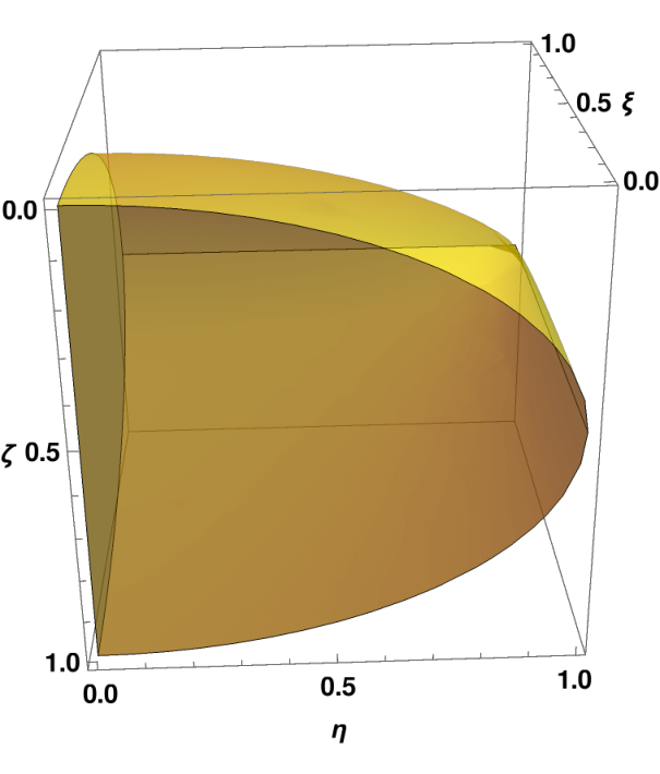
Refer to caption

Refer to caption

Figure 1: Dependence of gauge orbit variable ζi\zeta_{i} on ξ\xi and ηi\eta_{i}. (Left) Scatter plot of ζ\zeta with respect to ξ\xi and η\eta. (Right) Plot of ζ\zeta as a function of ξ\xi and η\eta given in eq. (29).

Naively, it might be expected that ζ1,ζ2∈[0,1]\zeta_{1},\zeta_{2}\in[0,1] Bonilla:2015eha. However, as can be seen from the scatter plot in Fig 1, ζi\zeta_{i} depends on ξi\xi_{i} and ηi\eta_{i}. In fact, it can be shown that value of ζi\zeta_{i} is bounded from above and below given by,

12​(1−1−ξ2​1−ηi2)≤ζi≤12​(1+1−ξ2​1−ηi2)\frac{1}{2}\left(1-\sqrt{1-\xi^{2}}\sqrt{1-\eta_{i}^{2}}\right)\leq\zeta_{i}\leq\frac{1}{2}\left(1+\sqrt{1-\xi^{2}}\sqrt{1-\eta_{i}^{2}}\right) (29)

where i∈{1,2}i\in\{1,2\}, |ξ|≤1|\xi|\leq 1 and ηi∈[0,1]\eta_{i}\in[0,1]. As can be seen in Fig 1, the dependence of ζi\zeta_{i} on ξ\xi and ηi\eta_{i} depicted in the scatter plot is captured exactly in eq. (29).

Substituting the above defined gauge orbit variables in eq. (28),

V4\displaystyle V_{4} =\displaystyle\ =\ r4​cos4⁡θ⁡(λ1+2​λ2​ξ2​cos⁡2​ω+λ3​ξ2+2​λ4​ξ​cos⁡ω)\displaystyle r^{4}\cos^{4}\theta\left(\lambda_{1}+2\lambda_{2}\xi^{2}\cos{2\omega}+\lambda_{3}\xi^{2}+2\lambda_{4}\,\xi\cos{\omega}\right) (30)
+r4​sin4⁡θ⁡(ρ1​(cos4⁡γ+sin4⁡γ)+ρ2​(η12​sin4⁡γ+η22​cos4⁡γ)CLOSE\displaystyle+r^{4}\sin^{4}\theta\left(\rho_{1}\left(\cos^{4}\gamma+\sin^{4}\gamma\right)+\rho_{2}\left(\eta_{1}^{2}\sin^{4}\gamma+\eta_{2}^{2}\cos^{4}\gamma\right)\right.
OPEN+ρ3​cos2⁡γ​sin2⁡γ+2​ρ4​η1​η2​cos⁡(θ1−θ2)​cos2⁡γ​sin2⁡γ)\displaystyle+\left.\rho_{3}\cos^{2}\gamma\sin^{2}\gamma+2\rho_{4}\eta_{1}\eta_{2}\cos(\theta_{1}-\theta_{2})\cos^{2}\gamma\sin^{2}\gamma\right)
+(α1+α3​(ζ1​cos2⁡γ+ζ2​sin2⁡γ))​r4​cos2⁡θ​sin2⁡θ\displaystyle+\left(\alpha_{1}+\alpha_{3}(\zeta_{1}\cos^{2}\gamma+\zeta_{2}\sin^{2}\gamma)\right)r^{4}\cos^{2}\theta\sin^{2}\theta
≡\displaystyle\equiv r4​(cos4⁡θ​f​(λ,ξ,ω)+sin4⁡θ​g​(ρ,γ,η1,2,θ1,2)+h⁡(α,γ,ζ1,2)​cos2⁡θ​sin2⁡θ)\displaystyle r^{4}\left(\cos^{4}\theta f(\lambda,\xi,\omega)+\sin^{4}\theta g(\rho,\gamma,\eta_{1,2},\theta_{1,2})+h(\alpha,\gamma,\zeta_{1,2})\cos^{2}\theta\sin^{2}\theta\right)

From copositivity criteria, it implies :

f⁡(λ,ξ,ω)>0f(\lambda,\xi,\omega)>0
g⁡(ρ,γ,η1,2,θ1,2)>0g(\rho,\gamma,\eta_{1,2},\theta_{1,2})>0
h⁡(α,γ,ζ1,2)+2​f⁡(λ,ξ,ω)​g​(ρ,γ,η1,2,θ1,2)>0h(\alpha,\gamma,\zeta_{1,2})+2\sqrt{f(\lambda,\xi,\omega)\>g(\rho,\gamma,\eta_{1,2},\theta_{1,2})}>0

These conditions should hold for all values of (ξ,ω,γ,η1,2,θ1,2,ζ1,2)(\xi,\omega,\gamma,\eta_{1,2},\theta_{1,2},\zeta_{1,2}). First two conditions are (14) and (20), evaluated in previous sections. For 2nd and 3rd condition, minimum of θ1,2\theta_{1,2} can again be absorbed in the sign of λ4\lambda_{4}.

α1+α3​(ζ1​cos2⁡γ+ζ2​sin2⁡γ)+f⁡(λ,ξ,ω)​g​(ρ,γ,η1,2)>0\alpha_{1}+\alpha_{3}(\zeta_{1}\cos^{2}\gamma+\zeta_{2}\sin^{2}\gamma)+\sqrt{f(\lambda,\xi,\omega)\>g(\rho,\gamma,\eta_{1,2})}>0 (31)

where ff and gg can be written as :

f≡λ1+2​λ2​ξ2​cos⁡2​ω+λ3​ξ2+2​λ4​ξ​cos⁡ωf\equiv\lambda_{1}+2\lambda_{2}\xi^{2}\cos{2\omega}+\lambda_{3}\xi^{2}+2\lambda_{4}\,\xi\cos{\omega}
g≡1(1+tan2⁡γ)2​(tan4⁡γ⁡(ρ1+ρ2​η22)+tan2⁡γ⁡(ρ3−2​|ρ4|​η1​η2)+ρ1+ρ2​η12)g\equiv\frac{1}{(1+\tan^{2}\gamma)^{2}}\left(\tan^{4}\gamma\left(\right.\rho_{1}+\rho_{2}\eta_{2}^{2}\right)+\tan^{2}\ \gamma\left(\rho_{3}-2|\rho_{4}|\eta_{1}\eta_{2}\right)+\left.\rho_{1}+\rho_{2}\eta_{1}^{2}\right) (32)

We now turn to symmetries to simplify further and reduce minimizing variables. We first try to minimize condition g⁡(ρ,γ,η1,2)g(\rho,\gamma,\eta_{1,2}) again but using symmetry arguments as an example. Note that gg is symmetric under the following operation:

cos⁡γ↔sin⁡γ,η1↔η2\cos\gamma\leftrightarrow\sin\gamma,\qquad\eta_{1}\leftrightarrow\eta_{2}

Thus, the minimum occurs at cos⁡γ=sin⁡γ\cos\gamma=\sin\gamma and η1=η2\eta_{1}=\eta_{2}, which yields :

g≡ρ3+2​ρ1+2​(ρ2−|ρ4|)​η124g\equiv\frac{\rho_{3}+2\rho_{1}+2(\rho_{2}-|\rho_{4}|)\eta_{1}^{2}}{4}

Plugging in the endpoints for η1\eta_{1}, we obtain two conditions :

g={ρ3+2​ρ14,ρ3+2​ρ1+2​(ρ2−|ρ4|)4}g=\left\{\frac{\rho_{3}+2\rho_{1}}{4},\frac{\rho_{3}+2\rho_{1}+2(\rho_{2}-|\rho_{4}|)}{4}\right\}

Previously, we minimized the condition for cos⁡γ=sin⁡γ\cos\gamma=\sin\gamma i.e. tan⁡γ=1\tan\gamma=1. Now, we will minimize gg for the endpoint, tan⁡γ=0\tan\gamma=0. Using the symmetry operations used above, it can be shown that minimizing the condition for other endpoint tan⁡γ=∞\tan\gamma=\infty is equivalent to case for tan⁡γ=0\tan\gamma=0. For this case, condition takes the form:

g≡ρ1+2​ρ2​η12g\equiv\rho_{1}+2\rho_{2}\eta_{1}^{2}

Again plugging in the endpoints for η1\eta_{1}, we obtain two conditions. We obtain a total of 4 conditions for minimizing gg, which exactly matches the conditions derived in sec. 4.2.

g:{ρ1,ρ1+ρ2,ρ3+2​ρ14,ρ3−2​|ρ4|+2​(ρ1+ρ2)4}g:\left\{\rho_{1},\,\rho_{1}+\rho_{2},\,\frac{\rho_{3}+2\rho_{1}}{4},\,\frac{\rho_{3}-2|\rho_{4}|+2(\rho_{1}+\rho_{2})}{4}\right\} (33)

Note that the 3rd condition is symmetric under the following operation:

ζ1↔ζ2,cos⁡γ↔sin⁡γ,η1↔η2\zeta_{1}\leftrightarrow\zeta_{2},\qquad\cos\gamma\leftrightarrow\sin\gamma,\qquad\eta_{1}\leftrightarrow\eta_{2}

Thus, the function takes its minimum value inside the gauge orbit space when:

ζ1=ζ2,cos⁡γ=sin⁡γ,η1=η2\zeta_{1}=\zeta_{2},\qquad\cos\gamma=\sin\gamma,\qquad\eta_{1}=\eta_{2}

Using the above symmetry arguments, the form of the 3rd condition is :

α1+α3​ζ1+f⁡(λ,ξ,ω)​(ρ3+2​ρ1+2​(ρ2−|ρ4|)​η12)>0\alpha_{1}+\alpha_{3}\zeta_{1}+\sqrt{f(\lambda,\xi,\omega)\>(\rho_{3}+2\rho_{1}+2(\rho_{2}-|\rho_{4}|)\eta_{1}^{2})}>0 (34)

For this case, the condition is monotonic in ζ1\zeta_{1} & η12\eta_{1}^{2} and are trivially minimized at endpoints of their range. This implies for α3<0\alpha_{3}<0, the most constraining condition corresponds to ζ1=ζ1m​a​x\zeta_{1}=\zeta_{1}^{max} and ζ1=ζim​i​n\zeta_{1}=\zeta_{i}^{min} for α3>0\alpha_{3}>0.

ζim​a​x=12​(1+1−ξ2​1−ηi2),ζim​i​n=12​(1−1−ξ2​1−ηi2)\zeta_{i}^{max}=\frac{1}{2}\left(1+\sqrt{1-\xi^{2}}\sqrt{1-\eta_{i}^{2}}\right),\quad\zeta_{i}^{min}=\frac{1}{2}\left(1-\sqrt{1-\xi^{2}}\sqrt{1-\eta_{i}^{2}}\right)

The minimum of ff has been evaluated in a previous section. This also yields corresponding value of ξ\xi and η1\eta_{1} that determines the value of ζim​a​x\zeta_{i}^{max} and ζim​i​n\zeta_{i}^{min}. This yields a set of 10 different conditions.

Consider an example for above discussion. Let us assume f⁡(λ,ξ,ω)f(\lambda,\xi,\omega) minimizes for ξ=|λ4|2​λ2+λ3\xi=\frac{|\lambda_{4}|}{2\lambda_{2}+\lambda_{3}} and η1=0\eta_{1}=0, then ζ1\zeta_{1} is given by :

⟹ζ1=12​(1±1−(|λ4|2​λ2+λ3)2)\implies\zeta_{1}=\frac{1}{2}\left(1\pm\sqrt{1-\left(\frac{|\lambda_{4}|}{2\lambda_{2}+\lambda_{3}}\right)^{2}}\right)

then the required inequality to be checked for vacuum stability becomes :

α1+α32​(1±1−λ42(2​λ2+λ3)2)+(λ1−λ422​λ2+λ3)​(ρ3+2​ρ1)>0\alpha_{1}+\frac{\alpha_{3}}{2}\left(1\pm\sqrt{1-\frac{\lambda_{4}^{2}}{(2\lambda_{2}+\lambda_{3})^{2}}}\right)+\sqrt{\left(\lambda_{1}-\frac{\lambda_{4}^{2}}{2\lambda_{2}+\lambda_{3}}\right)(\rho_{3}+2\rho_{1})}>0

We also need to minimize the 3rd condition for the edge surface of tan⁡γ\tan\gamma. For the case tan⁡γ=0\tan\gamma=0, 3rd condition takes the form:

α1+α3​ζ1+2​f⁡(λ,ξ,ω)​(ρ1+ρ2​η12)>0\alpha_{1}+\alpha_{3}\zeta_{1}+2\sqrt{f(\lambda,\xi,\omega)\>(\rho_{1}+\rho_{2}\eta_{1}^{2})}>0

The above condition can be minimized similarly as in case of tan⁡γ=1\tan\gamma=1, yielding a total of another 10 conditions.

Thus, minimizing the 3rd condition yields a set of 20 inequalities to be checked. We have finally derived all conditions required for the vacuum stability of the LRSM. The complete set of these necessary and sufficient conditions are collected below :

Analytic Conditions for Vacuum Stability in LRSM
f>0:{λ1(λ1−λ422​λ2+λ3)⟸2​λ2+λ3>|λ4|(λ1+λ3+2​(λ2−|λ4|))(λ1+λ3−2​λ2−λ424​λ2)⟸|4​λ2|>|λ4|\displaystyle{\rm f>0:\ }\begin{cases}\lambda_{1}\\ \left(\lambda_{1}-\frac{\lambda_{4}^{2}}{2\lambda_{2}+\lambda_{3}}\right)\qquad\quad\>\impliedby 2\lambda_{2}+\lambda_{3}>|\lambda_{4}|\\ \left(\lambda_{1}+\lambda_{3}+2(\lambda_{2}-|\lambda_{4}|)\right)\\ \left(\lambda_{1}+\lambda_{3}-2\lambda_{2}-\frac{\lambda_{4}^{2}}{4\lambda_{2}}\right)\impliedby|4\lambda_{2}|>|\lambda_{4}|\end{cases}
g>0:{ρ1,ρ1+ρ2,ρ3+2​ρ14,ρ3−2​|ρ4|+2​(ρ1+ρ2)4}\displaystyle g>0:\left\{\rho_{1},\,\rho_{1}+\rho_{2},\,\frac{\rho_{3}+2\rho_{1}}{4},\,\frac{\rho_{3}-2|\rho_{4}|+2(\rho_{1}+\rho_{2})}{4}\right\} (35)
α1+2​λ1​ρ1>0\displaystyle\alpha_{1}+2\sqrt{\lambda_{1}\rho_{1}}>0
α1+α3+2​λ1​ρ1>0\displaystyle\alpha_{1}+\alpha_{3}+2\sqrt{\lambda_{1}\rho_{1}}>0
α1+α32+2​λ1​(ρ1+ρ2)>0\displaystyle\alpha_{1}+\frac{\alpha_{3}}{2}+2\sqrt{\lambda_{1}(\rho_{1}+\rho_{2})}>0
α1+λ1​(ρ3+2​ρ1)>0\displaystyle\alpha_{1}+\sqrt{\lambda_{1}(\rho_{3}+2\rho_{1})}>0
α1+α3+λ1​(ρ3+2​ρ1)>0\displaystyle\alpha_{1}+\alpha_{3}+\sqrt{\lambda_{1}(\rho_{3}+2\rho_{1})}>0
α1+α32+λ1​(ρ3−2​|ρ4|+2​(ρ1+ρ2))>0\displaystyle\alpha_{1}+\frac{\alpha_{3}}{2}+\sqrt{\lambda_{1}(\rho_{3}-2|\rho_{4}|+2(\rho_{1}+\rho_{2}))}>0
α1+α32​(1±1−λ42(2​λ2+λ3)2)+2​(λ1−λ422​λ2+λ3)​ρ1>0\displaystyle\alpha_{1}+\frac{\alpha_{3}}{2}\left(1\pm\sqrt{1-\frac{\lambda_{4}^{2}}{(2\lambda_{2}+\lambda_{3})^{2}}}\right)+2\sqrt{\left(\lambda_{1}-\frac{\lambda_{4}^{2}}{2\lambda_{2}+\lambda_{3}}\right)\rho_{1}}>0
α1+α32+2​(λ1−λ422​λ2+λ3)​(ρ1+ρ2)>0\displaystyle\alpha_{1}+\frac{\alpha_{3}}{2}+2\sqrt{\left(\lambda_{1}-\frac{\lambda_{4}^{2}}{2\lambda_{2}+\lambda_{3}}\right)(\rho_{1}+\rho_{2})}>0
α1+α32​(1±1−λ42(2​λ2+λ3)2)+(λ1−λ422​λ2+λ3)​(ρ3+2​ρ1)>0\displaystyle\alpha_{1}+\frac{\alpha_{3}}{2}\left(1\pm\sqrt{1-\frac{\lambda_{4}^{2}}{(2\lambda_{2}+\lambda_{3})^{2}}}\right)+\sqrt{\left(\lambda_{1}-\frac{\lambda_{4}^{2}}{2\lambda_{2}+\lambda_{3}}\right)(\rho_{3}+2\rho_{1})}>0
α1+α32+(λ1−λ422​λ2+λ3)​(ρ3−2​|ρ4|+2​(ρ1+ρ2))>0\displaystyle\alpha_{1}+\frac{\alpha_{3}}{2}+\sqrt{\left(\lambda_{1}-\frac{\lambda_{4}^{2}}{2\lambda_{2}+\lambda_{3}}\right)(\rho_{3}-2|\rho_{4}|+2(\rho_{1}+\rho_{2}))}>0
α1+α32+2​(λ1+λ3−2​λ2−λ424​λ2)​Min​(g)>0\displaystyle\alpha_{1}+\frac{\alpha_{3}}{2}+2\sqrt{\left(\lambda_{1}+\lambda_{3}-2\lambda_{2}-\frac{\lambda_{4}^{2}}{4\lambda_{2}}\right)\>\textbf{Min}(g)}>0
α1+α32+2​(λ1+λ3+2​(λ2−|λ4|))​Min​(g)>0\displaystyle\alpha_{1}+\frac{\alpha_{3}}{2}+2\sqrt{\left(\lambda_{1}+\lambda_{3}+2(\lambda_{2}-|\lambda_{4}|)\right)\>\textbf{Min}(g)}>0

For using these conditions, we first ensure ff and gg should be strictly positive at all minima. For some conditions in ff, we have the following structure p⟸qp\impliedby q. This implies condition pp only needs to be checked if and only if condition qq is true. We then check rest of the conditions based on minimum value of ff and gg.

5 Symmetry Breaking and Desirable Vacuum

A BFB potential does not necessarily leads to correct symmetry breaking yielding the correct ground state of the Higgs potential. Recently, some useful conditions (though not necessary) for a good vacuum in the left-right model were derived for a limited parameter space in Dev:2018foq. Gauge-independent criteria to obtain a good vacuum was also proposed.

⟨Φ⟩≠0\langle\Phi\rangle\neq 0
det⁡⟨ΔR⟩=det⁡⟨ΔL⟩=0\operatorname{det}\langle\Delta_{R}\rangle=\operatorname{det}\langle\Delta_{L}\rangle=0
⟨ΔR⟩≠⟨ΔL⟩\langle\Delta_{R}\rangle\neq\langle\Delta_{L}\rangle

The first condition leads to non-zero expectation for Higgs VEV in the Standard Model. The second condition is required for U​(1)e​mU(1)_{em} not to be broken. The third condition is required for broken parity at low energies. Although reference Dev:2018foq specifies 4 conditions for a good vacuum but effectively only 3 conditions are required. As their condition ⟨ΔR⟩≠0​ or ​⟨ΔL⟩≠0\langle\Delta_{R}\rangle\neq 0\text{ or }\langle\Delta_{L}\rangle\neq 0 for good vacuum is contained in ⟨ΔR⟩≠⟨ΔL⟩\langle\Delta_{R}\rangle\neq\langle\Delta_{L}\rangle.

In this section, we derive some useful conditions for scalar potential to exhibit correct spontaneous symmetry breaking (SSB) and specify the gauge-independent criteria for correct vacuum in more general form. Using the VEV structure of the scalar fields eq. (10) in the general scalar potential eq. (11),

V\displaystyle V =\displaystyle\ =\ −(κ12+κ22)2​μ12−2​κ1​κ2​μ22​cos⁡(θ2)−μ32​(vL2+vR2)+(κ12+κ22)24​λ1\displaystyle-\frac{\left(\kappa_{1}^{2}+\kappa_{2}^{2}\right)}{2}\mu_{1}^{2}-2\kappa_{1}\kappa_{2}\mu_{2}^{2}\cos(\theta_{2})-\mu_{3}^{2}\left(v_{L}^{2}+v_{R}^{2}\right)+\frac{\left(\kappa_{1}^{2}+\kappa_{2}^{2}\right)^{2}}{4}\lambda_{1} (36)
+2​κ12​κ22​λ2​cos⁡(2​θ2)+κ1​κ2​(κ12+κ22)​λ4​cos⁡(θ2)+κ12​κ22​λ3\displaystyle+2\kappa_{1}^{2}\kappa_{2}^{2}\lambda_{2}\cos(2\theta_{2})+\kappa_{1}\kappa_{2}\left(\kappa_{1}^{2}+\kappa_{2}^{2}\right)\lambda_{4}\cos(\theta_{2})+\kappa_{1}^{2}\kappa_{2}^{2}\lambda_{3}
+ρ1​(vL4+vR4)+ρ3​vL2​vR2\displaystyle+\rho_{1}\left(v_{L}^{4}+v_{R}^{4}\right)+\rho_{3}v_{L}^{2}v_{R}^{2}
+α1​(κ12+κ22)2​(vL2+vR2)+α3​κ222​(vL2+vR2)\displaystyle+\alpha_{1}\frac{\left(\kappa_{1}^{2}+\kappa_{2}^{2}\right)}{2}\left(v_{L}^{2}+v_{R}^{2}\right)+\alpha_{3}\frac{\kappa_{2}^{2}}{2}\left(v_{L}^{2}+v_{R}^{2}\right)

For boundedness, the quartic part of the potential can be written as:

V4\displaystyle V_{4} ≡\displaystyle\equiv r4​(fS​S​B​(λ,ξ,ω)​cos4⁡θ+gS​S​B​(ρ,γ,θ1,2)​sin4⁡θ+hS​S​B​(α,γ,ζ1,2)​cos2⁡θ​sin2⁡θ)\displaystyle r^{4}\left(f_{SSB}(\lambda,\xi,\omega)\cos^{4}\theta+g_{SSB}(\rho,\gamma,\theta_{1,2})\sin^{4}\theta+h_{SSB}(\alpha,\gamma,\zeta_{1,2})\cos^{2}\theta\sin^{2}\theta\right) (37)

where parametrizing variables are defined in accordance with section 4.3. To obtain necessary and sufficient conditions for correct symmetry breaking, the minimum from the potential VS​S​BV_{SSB} should be deeper than the one obtained from the general potential. Using eq. (9), the required condition can be written as :

−g​μ14−h​μ12​μ22+f​μ244​f​g−h2>−gS​S​B​μ14−hS​S​B​μ12​μ22+fS​S​B​μ244​fS​S​B​gS​S​B−hS​S​B2-\frac{g\mu_{1}^{4}-h\mu_{1}^{2}\mu_{2}^{2}+f\mu_{2}^{4}}{4fg-h^{2}}>-\frac{g_{SSB}\mu_{1}^{4}-h_{SSB}\mu_{1}^{2}\mu_{2}^{2}+f_{SSB}\mu_{2}^{4}}{4f_{SSB}\>g_{SSB}-h_{SSB}^{2}} (38)

The above relation needs to be minimized for the entire gauge orbit parameter space. Due to the non-linearity of the orbit variables, this is not analytically tractable.

The important observation in this work is that the conditions sufficient for a general potential to lead to a good vacuum after SSB can be obtained by requiring VEV aligned scalar potential to dominate the general scalar potential i.e. V≥VS​S​BV\geq V_{SSB}. This is a stronger condition than eq. (38) and using eq. (30), (37) can be written as :

(f−fS​S​B)​cos4⁡θ+(g−gS​S​B)​sin4⁡θ+(h−hS​S​B)​cos2⁡θ​sin2⁡θ≥0(f-f_{SSB})\cos^{4}\theta+(g-g_{SSB})\sin^{4}\theta+(h-h_{SSB})\cos^{2}\theta\sin^{2}\theta\geq 0 (39)

Thus, for VEV structure in eq. (10) to be the global minima of the theory, following conditions are required :

f≥fS​S​B,g≥gS​S​B\displaystyle f\geq f_{SSB},\quad g\geq g_{SSB} (40)
h−hS​S​B+2​(f−fS​S​B)​(g−gS​S​B)≥0\displaystyle h-h_{SSB}+2\sqrt{(f-f_{SSB})\>(g-g_{SSB})}\geq 0 (41)

It is also required that VS​S​BV_{SSB} exhibits stable vaccum, which implies :

fS​S​B>0,gS​S​B>0,hS​S​B+2​fS​S​B​gS​S​B>0\displaystyle f_{SSB}>0,\quad g_{SSB}>0,\quad h_{SSB}+2\sqrt{f_{SSB}\>g_{SSB}}>0 (42)

We begin by noticing that in eq. (36), fS​S​Bf_{SSB} takes the same form as f⁡(λ,ξ,ω)f(\lambda,\xi,\omega) for the general potential. VEV condition ⟨Φ⟩≠0\langle\Phi\rangle\neq 0 translates to r​cos⁡θ≠0r\cos{\theta}\neq 0. It is satisfied as long as λ\lambda sector is bounded from below. This implies all the conditions found for λ\lambda sector are required for existence of a good vacuum. It also implies f=fS​S​Bf=f_{SSB} trivially satisfies condition for correct symmetry breaking.
On the other hand, gS​S​Bg_{SSB} has η1,2=0\eta_{1,2}=0.

Tr​[⟨ΔL⟩​⟨ΔL⟩]=0⟹η1=0\text{Tr}[\langle\Delta_{L}\rangle\langle\Delta_{L}\rangle]=0\quad\implies\eta_{1}=0
Tr​[⟨ΔR⟩​⟨ΔR⟩]=0⟹η2=0\text{Tr}[\langle\Delta_{R}\rangle\langle\Delta_{R}\rangle]=0\quad\implies\eta_{2}=0

Therefore, coefficients of ρ2\rho_{2} and ρ4\rho_{4} vanish leading to following form of gg (See eq. (32)):

gS​S​B≡1(1+tan2⁡γ)2​(ρ1​tan4⁡γ+ρ3​tan2⁡γ+ρ1)g_{SSB}\equiv\frac{1}{(1+\tan^{2}\gamma)^{2}}\left(\rho_{1}\tan^{4}\gamma+\rho_{3}\tan^{2}\ \gamma+\rho_{1}\right)

The minimum for this expression occurs at tan2⁡γ=0​ or ​1\tan^{2}\gamma=0\text{ or }1. We require ⟨ΔL⟩<⟨ΔR⟩\langle\Delta_{L}\rangle<\langle\Delta_{R}\rangle which can be easily shown equivalent to :

Tr​[⟨ΔL⟩​⟨ΔL†⟩]<Tr​[⟨ΔR⟩​⟨ΔR†⟩]\text{Tr}[\langle\Delta_{L}\rangle\langle\Delta_{L}^{\dagger}\rangle]<\text{Tr}[\langle\Delta_{R}\rangle\langle\Delta_{R}^{\dagger}\rangle]

So according to the chosen parametrization, the preferred minima is tan2⁡γ=0\tan^{2}\gamma=0. We know from sec. 2.2, condition with less positive value dominates the minima. Thus, this condition should dominate over the other minima i.e tan2⁡γ=1\tan^{2}\gamma=1 in gS​S​Bg_{SSB}. Thus, we require

ρ3+2​ρ14≥ρ1⟹ρ3−2​ρ1≥0\frac{\rho_{3}+2\rho_{1}}{4}\geq\rho_{1}\implies\rho_{3}-2\rho_{1}\geq 0

After requiring the internal structure of the VEV alignment, we want eq. (40) to hold i.e. g≥gS​S​Bg\geq g_{SSB} should hold. The minimum of gS​S​Bg_{SSB} occurs for ρ1>0\rho_{1}>0. This condition should dominate other possible minima of the general potential. Using minimum conditions from eq. (33),

ρ1+ρ2≥ρ1⟹ρ2≥0\rho_{1}+\rho_{2}\geq\rho_{1}\implies\rho_{2}\geq 0
ρ3+2​ρ14≥ρ1⟹ρ3−2​ρ1≥0\frac{\rho_{3}+2\rho_{1}}{4}\geq\rho_{1}\implies\rho_{3}-2\rho_{1}\geq 0
ρ3−2​|ρ4|+2​(ρ1+ρ2)4≥ρ1⟹|ρ4|≤ρ3−2​ρ12+ρ2\frac{\rho_{3}-2|\rho_{4}|+2(\rho_{1}+\rho_{2})}{4}\geq\rho_{1}\implies|\rho_{4}|\leq\frac{\rho_{3}-2\rho_{1}}{2}+\rho_{2}

Since f=fS​S​Bf=f_{SSB}, eq. (41) implies h≥hS​S​Bh\geq h_{SSB}.

α1+α3​(ζ1​cos2⁡γ+ζ2​sin2⁡γ)≥α1+α3​(ζ1S​S​B​cos2⁡γ+ζ2S​S​B​sin2⁡γ)\alpha_{1}+\alpha_{3}(\zeta_{1}\cos^{2}\gamma+\zeta_{2}\sin^{2}\gamma)\geq\alpha_{1}+\alpha_{3}(\zeta_{1}^{SSB}\cos^{2}\gamma+\zeta_{2}^{SSB}\sin^{2}\gamma)

Note that since ηi=0\eta_{i}=0 for VS​S​BV_{SSB}, ζi≠ζiS​S​B\zeta_{i}\neq\zeta_{i}^{SSB}. The condition above is monotonic in ζ\zeta ’s and the endpoints of their range can be substituted depending on the sign of α3\alpha_{3}.

α32​(1−Sgn​(α3)​1−ξ2​1−ηi2)≥α32​(1−Sgn​(α3)​1−ξ2)\frac{\alpha_{3}}{2}\left(1-\textbf{Sgn}(\alpha_{3})\sqrt{1-\xi^{2}}\sqrt{1-\eta_{i}^{2}}\right)\geq\frac{\alpha_{3}}{2}\left(1-\textbf{Sgn}(\alpha_{3})\sqrt{1-\xi^{2}}\right)

As can be seen directly, the above condition holds true for all ξ\xi, η\eta and α3\alpha_{3}. Similarly, for vacuum stability condition to hold true, we require :

α1+α32​ζ+2​f⁡(λ,ξ,ω)​ρ1>0\alpha_{1}+\frac{\alpha_{3}}{2}\zeta+2\sqrt{f(\lambda,\xi,\omega)\>\rho_{1}}>0 (43)

where, ζ=(1−Sgn​(α3)​1−ξ∗2)\zeta=\left(1-\textbf{Sgn}(\alpha_{3})\sqrt{1-\xi_{*}^{2}}\right) and ξ∗\xi_{*} equals the value of ξ\xi that minimizes f⁡(λ,ξ,ω)f(\lambda,\xi,\omega). The minimization of ff has been covered in sec. 4.1.

For non-zero field values to be the global minimum (refer sec. 2.2), we also require eq. (6),(7) and (8) to hold. For non-zero ⟨Φ⟩\langle\Phi\rangle and ⟨ΔR⟩\langle\Delta_{R}\rangle, we require :

2​Min​[fS​S​B]​μ32−Min​[hS​S​B]​μ¯12>02\>\textbf{Min}[f_{SSB}]\mu_{3}^{2}-\textbf{Min}[h_{SSB}]\bar{\mu}_{1}^{2}>0
2​Min​[gS​S​B]​μ¯12−Min​[hS​S​B]​μ32>02\>\textbf{Min}[g_{SSB}]\bar{\mu}_{1}^{2}-\textbf{Min}[h_{SSB}]\mu_{3}^{2}>0 (44)

where,

μ¯12=μ12+2​σ​μ22,σ=ξ​cos⁡ω\bar{\mu}_{1}^{2}=\mu_{1}^{2}+2\sigma\mu_{2}^{2},\quad\quad\sigma=\xi\cos\omega

and

2​Min​[fS​S​B]​Min​[gS​S​B]−‖Min​[hS​S​B]‖>02\sqrt{\textbf{Min}[f_{SSB}]\>\textbf{Min}[g_{SSB}]}-\mathbf{||}\textbf{Min}[h_{SSB}]\mathbf{||}>0

Here, expression for μ¯12\bar{\mu}_{1}^{2} has been obtained by using parametrization from sec. (4.1) to relevant mass-squared terms in the scalar potential. Thus, the complete set of conditions sufficient to obtain a correct vacuum after SSB in left-right symmetric model are stated below:

Analytic Conditions for Symmetry Breaking to Correct Vacuum
fSSB>0:{λ1>0,ξ=σ=0,(λ1−λ422​λ2+λ3)>0⟸0<ξ=|λ4|2​λ2+λ3<1,σ=−λ42​λ2+λ3,(λ1+λ3+2(λ2−|λ4|))>0,ξ=1,σ=−Sgn(λ4),(λ1+λ3−2λ2−λ424​λ2)>0⟸|4λ2|>|λ4|,ξ=1,σ=−λ44​λ2,\displaystyle{\rm f_{SSB}>0:\ }\begin{cases}\lambda_{1}>0,\quad\xi=\sigma=0\,,\\ \left(\lambda_{1}-\frac{\lambda_{4}^{2}}{2\lambda_{2}+\lambda_{3}}\right)>0\impliedby 0<\xi=\frac{|\lambda_{4}|}{2\lambda_{2}+\lambda_{3}}<1,\quad\sigma=-\frac{\lambda_{4}}{2\lambda_{2}+\lambda_{3}},\\ \left(\lambda_{1}+\lambda_{3}+2(\lambda_{2}-|\lambda_{4}|)\right)>0,\quad\xi=1,\>\sigma=-\textbf{Sgn}(\lambda_{4})\,,\\ \left(\lambda_{1}+\lambda_{3}-2\lambda_{2}-\frac{\lambda_{4}^{2}}{4\lambda_{2}}\right)>0\impliedby|4\lambda_{2}|>|\lambda_{4}|,\quad\xi=1,\>\sigma=-\frac{\lambda_{4}}{4\lambda_{2}},\end{cases}
ρ1>0,ρ2>0,ρ3>2​ρ1,|ρ4|<ρ3−2​ρ12+ρ2\displaystyle\rho_{1}>0,\quad\rho_{2}>0,\quad\rho_{3}>2\rho_{1},\quad|\rho_{4}|<\frac{\rho_{3}-2\rho_{1}}{2}+\rho_{2}
α1+2​λ1​ρ1>0\displaystyle\alpha_{1}+2\sqrt{\lambda_{1}\rho_{1}}>0
α1+α3+2​λ1​ρ1>0\displaystyle\alpha_{1}+\alpha_{3}+2\sqrt{\lambda_{1}\rho_{1}}>0
α1+α32​(1±1−λ42(2​λ2+λ3)2)+2​(λ1−λ422​λ2+λ3)​ρ1>0\displaystyle\alpha_{1}+\frac{\alpha_{3}}{2}\left(1\pm\sqrt{1-\frac{\lambda_{4}^{2}}{(2\lambda_{2}+\lambda_{3})^{2}}}\right)+2\sqrt{\left(\lambda_{1}-\frac{\lambda_{4}^{2}}{2\lambda_{2}+\lambda_{3}}\right)\rho_{1}}>0
α1+α32+2​(λ1+λ3−2​λ2−λ424​λ2)​ρ1>0\displaystyle\alpha_{1}+\frac{\alpha_{3}}{2}+2\sqrt{\left(\lambda_{1}+\lambda_{3}-2\lambda_{2}-\frac{\lambda_{4}^{2}}{4\lambda_{2}}\right)\>\rho_{1}}>0
α1+α32+2​(λ1+λ3+2​(λ2−|λ4|))​ρ1>0\displaystyle\alpha_{1}+\frac{\alpha_{3}}{2}+2\sqrt{\left(\lambda_{1}+\lambda_{3}+2(\lambda_{2}-|\lambda_{4}|)\right)\>\rho_{1}}>0
μ¯12=μ12+2​σ​μ22\displaystyle\bar{\mu}_{1}^{2}=\mu_{1}^{2}+2\sigma\mu_{2}^{2}
2​Min​[fS​S​B]​ρ1−||α1+α32​(1−Sgn​(α3)​1−ξ2)||>0\displaystyle 2\sqrt{\textbf{Min}[f_{SSB}]\>\rho_{1}}-\left|\left|\alpha_{1}+\frac{\alpha_{3}}{2}\left(1-\textbf{Sgn}(\alpha_{3})\sqrt{1-\xi^{2}}\right)\right|\right|>0
2​Min​[fS​S​B]​μ32−[α1+α32​(1−Sgn​(α3)​1−ξ2)]​μ¯12>0\displaystyle 2\>\textbf{Min}[f_{SSB}]\mu_{3}^{2}-\left[\alpha_{1}+\frac{\alpha_{3}}{2}\left(1-\textbf{Sgn}(\alpha_{3})\sqrt{1-\xi^{2}}\right)\right]\bar{\mu}_{1}^{2}>0
2​ρ1​μ¯12−[α1+α32​(1−Sgn​(α3)​1−ξ2)]​μ32>0\displaystyle 2\rho_{1}\bar{\mu}_{1}^{2}-\left[\alpha_{1}+\frac{\alpha_{3}}{2}\left(1-\textbf{Sgn}(\alpha_{3})\sqrt{1-\xi^{2}}\right)\right]\mu_{3}^{2}>0

For using these conditions, we first ensure fS​S​Bf_{SSB} should be strictly positive at all minima. For some conditions in ff, we have the following structure p⟸q,ξ=value1,σ=value2p\impliedby q,\>\xi=\texttt{value1},\>\sigma=\texttt{value2}. This implies condition pp only needs to be checked if and only if condition qq is true. It also yields a corresponding values of ξ\xi and σ\sigma to be used in the last three conditions. We then check rest of the conditions based on minimum value of fS​S​Bf_{SSB}.

We would like to assert the usefulness of these conditions. Using the above conditions not only ensures the boundedness of the potential but also gives the minimum with desired VEV alignment. The results derived here are general in nature and reduce to those obtained in Dev:2018foq for their choice of parameters44 4 Setting λ2,4\lambda_{2,4}, ρ4\rho_{4}, αi\alpha_{i}’s and βi\beta_{i}’s to 0. In Dev:2018foq, their derived conditions for good vacuum are asserted to be only sufficient but not necessary and same holds for our case. Even with good vacuum conditions, they do not get a correct vacuum in their numerical study at all times. This possibly happens due to the parameter range of non-zero αi\alpha_{i}’s in their numerical analysis that leads to the violation of condition on mass-squares μ2{\mu}^{2} derived in this work.

Given the treatment here, we can also generalize the gauge-independent conditions for correct vacuum in the left-right symmetric model as:

Tr​[⟨Φ⟩​⟨Φ⟩]≠0\displaystyle\text{Tr}[\langle\Phi\rangle\langle\Phi\rangle]\neq 0
Tr​[⟨ΔL⟩​⟨ΔL⟩]=Tr​[⟨ΔR⟩​⟨ΔR⟩]=0\displaystyle\text{Tr}[\langle\Delta_{L}\rangle\langle\Delta_{L}\rangle]=\text{Tr}[\langle\Delta_{R}\rangle\langle\Delta_{R}\rangle]=0 (45)
Tr​[⟨ΔL⟩​⟨ΔL†⟩]<Tr​[⟨ΔR⟩​⟨ΔR†⟩]\displaystyle\text{Tr}[\langle\Delta_{L}\rangle\langle\Delta_{L}^{\dagger}\rangle]<\text{Tr}[\langle\Delta_{R}\rangle\langle\Delta_{R}^{\dagger}\rangle]

Figure 2: Numerical minimization of the scalar potential of LRSM. The figures are plotted for different pair of quartic couplings with values ranging from (−5,5)(-5,5) and with grid pixel size of 0.1×0.10.1\times 0.1, with other quartics being set according to benchmark in Sec 6. The yellow region indicates an unbounded potential. The green region indicates the existence of a global minimum but not with the required VEV structure. The blue region indicates the existence of a global minimum with the required VEV structure.

6 Numerical Comparison

We use the following benchmark values to study the numerical minimization of the potential and its agreement with the conditions obtained in this work.

μ12,μ22,μ32\displaystyle\mu_{1}^{2},\>\mu_{2}^{2},\>\mu_{3}^{2}\> ≡\displaystyle\equiv (1,0.25,1)​TeV2\displaystyle(1,0.25,1)\,\text{TeV}^{2}
λ1,λ2,λ3,λ4\displaystyle\lambda_{1},\>\lambda_{2},\>\lambda_{3},\>\lambda_{4} ≡\displaystyle\equiv (1,0.5,3,−0.5)\displaystyle(1,0.5,3,-0.5)
ρ1,ρ2,ρ3,ρ4\displaystyle\rho_{1},\>\rho_{2},\>\rho_{3},\>\rho_{4} ≡\displaystyle\equiv (1,0.5,3,−0.5)\displaystyle(1,0.5,3,-0.5)
α1,α2,α3\displaystyle\alpha_{1},\>\alpha_{2},\>\alpha_{3} ≡\displaystyle\equiv (0.5,0,0.5)\displaystyle(0.5,0,0.5)
β1,β2,β3\displaystyle\beta_{1},\>\beta_{2},\>\beta_{3} ≡\displaystyle\equiv (0,0,0)\displaystyle(0,0,0)

In fig 2, the potential is minimized for a pair of quartics with other couplings set according to the benchmark values. The minimization was performed with the NMinimize function with NelderMead, DifferentialEvolution and SimulatedAnnealing method in Mathematica. The pixel size of the grid is 0.1×0.10.1\times 0.1. With each parameter running from (−5,5)(-5,5) yields a 50×5050\times 50 matrix. The yellow region has unbounded minima that violates the BFB conditions. The green region is bounded and has a global minimum but with an incorrect VEV alignment. In blue region, the potential undergoes correct sponataneous symmetry breaking to the desired VEV structure of the vacuum. This vacuum is stable and is phenomenologically viable.

We would like to assert that the results shown in fig 2 are in complete agreement with the vacuum stability and correct vacuum conditions obtained in this work. It should also be noted that although conditions to exhibit SSB to correct vaccum were derived using a stronger condition, they match results from numerical minimization remarkably.

7 Renormalization Group Equations Analysis

In a general case of randomly selected initial values, the evolution of quartic couplings according to the renormalization group equations (RGEs) for the model can lead to their running outside the allowed parameter space. Constraining the running of the quartic couplings to satisfy the vacuum stability conditions upto a certain high energy scale ensures the boundedness of the potential. In this section, we discuss some more constraints on the quartic couplings before we present an example study to demostrate the usefulness of the conditions derived earlier.

7.1 Mass Spectrum & Unitarity Bounds

Along with BFB conditions and correct symmetry breaking, it’s necessary to check that the potential exhibits a physical scalar mass spectrum. The scalar mass spectrum of the LRSM has 14 physical particles. It includes 8 electrically neutral 55 5 It contains two massless neutral degrees of freedom absorbed as the longitudinal polarization modes of physical gauge bosons., four singly-charged and four doubly-charged Higgs bosons. The scalar mass spectrum for LRSM is given belowDuka:1999uc; Chakrabortty:2016wkl:

MH002\displaystyle M_{H_{0}^{0}}^{2} =\displaystyle= 2​(λ1−α124​ρ1)​κ+2,\displaystyle 2\left(\lambda_{1}-\frac{\alpha_{1}^{2}}{4\rho_{1}}\right)\kappa_{+}^{2},
MH2±2≃MA102≃MH102\displaystyle M_{H_{2}^{\pm}}^{2}\simeq M_{A_{1}^{0}}^{2}\simeq M_{H_{1}^{0}}^{2} =\displaystyle= 12​α3​vR2,\displaystyle\frac{1}{2}\alpha_{3}v_{R}^{2},
MH202\displaystyle M_{H_{2}^{0}}^{2} =\displaystyle= 2​ρ1​vR2,\displaystyle 2\rho_{1}v_{R}^{2},
MH1±⁣±2≃MH1±2≃MA202=MH302\displaystyle M_{H_{1}^{\pm\pm}}^{2}\simeq M_{H_{1}^{\pm}}^{2}\simeq M_{A_{2}^{0}}^{2}=M_{H_{3}^{0}}^{2} =\displaystyle= 12​(ρ3−2​ρ1)​vR2,\displaystyle\frac{1}{2}(\rho_{3}-2\rho_{1})v_{R}^{2},
MH2±⁣±2\displaystyle M_{H_{2}^{\pm\pm}}^{2} =\displaystyle= 2​ρ2​vR2+12​α3​κ+2\displaystyle 2\rho_{2}v_{R}^{2}+\frac{1}{2}\alpha_{3}\kappa_{+}^{2}

where κ+2=κ12+κ22\kappa_{+}^{2}=\kappa_{1}^{2}+\kappa_{2}^{2}. The lightest neutral scalar MH00M_{H_{0}^{0}} that only depends on the VEV of bidoublet Φ\Phi is identified as the SM Higgs boson. We have taken the best fit value of MH00=mh=125M_{H_{0}^{0}}=m_{h}=125 GeV Aad:2015zhl. H10H_{1}^{0}, A10A_{1}^{0} and H2±H_{2}^{\pm} are the CP-even and CP-odd neutral components and the two singly-charged scalars respectively from the bidoublet Φ\Phi. H20H_{2}^{0}, H30H_{3}^{0}, A20A_{2}^{0}, H1±H_{1}^{\pm}, H1±⁣±H_{1}^{\pm\pm} and H2±⁣±H_{2}^{\pm\pm} are the two CP-even and one CP-odd neutral components, 2 singly-charged and 4 doubly-charged scalars respectively from the triplets ΔL\Delta_{L} and ΔR\Delta_{R}.

There are strong experimental bounds on most scalar masses in LRSM. This places lower bounds on the allowed values of corresponding quartic couplings in the potential as a function of the breaking scale. The heavy neutral scalars H10H_{1}^{0}, A10A_{1}^{0} can contribute to Bd−B¯dB_{d}-\overline{B}_{d}, Bs−B¯dB_{s}-\overline{B}_{d} and K0−K¯0K_{0}-\overline{K}_{0} mixings due to presence of tree-level FCNC couplings to the SM quarks in LRSM. Thus, there are stringent limits on their masses from the FCNC constraints Ecker:1983uh; Zhang:2007da; Maiezza:2010ic.

MH10,A10>15​ TeVM_{H_{1}^{0},A_{1}^{0}}>15\text{ TeV}

The cleanest detection channel for doubly-charged Higgs bosons is its decay to same-sign charged dilepton pairs . The current bounds on mass limits are from LHC 13 TeV run data Aaboud:2017qph; CMS-PAS-HIG-16-036, which largely depends on charged lepton flavors involved in the decay process :

MH1±⁣±≳(770−870)​ GeVMH2±⁣±≳(660−760)​ GeVM_{H_{1}^{\pm\pm}}\gtrsim(770-870)\text{ GeV}\qquad M_{H_{2}^{\pm\pm}}\gtrsim(660-760)\text{ GeV}

Parameter space for quartic couplings can be further squeezed by requiring tree-level unitarity to be preserved in a variety of scattering process. We consider the unitarity bounds only from 2-body scalar scattering processes Chakrabortty:2016wkl, given below :

λ1<4​π/3,(λ1+4​λ2+2​λ3)<4​π,\displaystyle\lambda_{1}<4\pi/3,~(\lambda_{1}+4\lambda_{2}+2\lambda_{3})<4\pi,
(λ1−4​λ2+2​λ3)<4​π,\displaystyle(\lambda_{1}-4\lambda_{2}+2\lambda_{3})<4\pi,
λ4<4​π/3,\displaystyle\lambda_{4}<4\pi/3,
α1<8​π,α2<4​π,(α1+α3)<8​π,\displaystyle\alpha_{1}<8\pi,~\alpha_{2}<4\pi,~(\alpha_{1}+\alpha_{3})<8\pi,
ρ1<4​π/3,(ρ1+ρ2)<2​π,ρ2<2​2​π,\displaystyle\rho_{1}<4\pi/3,~(\rho_{1}+\rho_{2})<2\pi,~\rho_{2}<2\sqrt{2}\pi,
ρ3<8​π,ρ4<2​2​π\displaystyle\rho_{3}<8\pi,~\rho_{4}<2\sqrt{2}\pi

7.2 Example Study

Figure 3: RG running of the quartic couplings for the benchmark in sec 7.2 from vR=26.8v_{R}=26.8 TeV, with rg=gRgL=1.2r_{g}=\frac{g_{R}}{g_{L}}=1.2.

We use the following benchmark values for RGE running of the quartic couplings.

μ12,μ22,μ32\displaystyle\mu_{1}^{2},\>\mu_{2}^{2},\>\mu_{3}^{2}\> ≡\displaystyle\equiv ((8.48)2,0,(11.99)2)​ TeV2\displaystyle((8.48)^{2},0,(11.99)^{2})\text{ TeV}^{2}
λ1,λ2,λ3,λ4\displaystyle\lambda_{1},\>\lambda_{2},\>\lambda_{3},\>\lambda_{4} ≡\displaystyle\equiv (0.0625,0,0,0)\displaystyle(0.0625,0,0,0)
ρ1,ρ2,ρ3,ρ4\displaystyle\rho_{1},\>\rho_{2},\>\rho_{3},\>\rho_{4} ≡\displaystyle\equiv (0.01,0.0005,0.0226,0)\displaystyle(0.01,0.0005,0.0226,0) (46)
α1,α2,α3\displaystyle\alpha_{1},\>\alpha_{2},\>\alpha_{3} ≡\displaystyle\equiv (0.01,0,0.64)\displaystyle(0.01,0,0.64)
β1,β2,β3\displaystyle\beta_{1},\>\beta_{2},\>\beta_{3} ≡\displaystyle\equiv (0,0,0)\displaystyle(0,0,0)

The above benchmark is in complete agreement with the current experimental bounds on the scalar masses at the breaking scale.

κ+=κ12+κ22=246​ GeV,vL=0​ TeV,vR=26.8​ TeV\kappa_{+}=\sqrt{\kappa_{1}^{2}+\kappa_{2}^{2}}=246\text{ GeV},\>v_{L}=0\text{ TeV},\>v_{R}=26.8\text{ TeV}

Most importantly the ground state of the potential exhibits correct VEV structure of the theory at the right-handed breaking scale vRv_{R}. This is evident as the benchmark eq. (7.2) satifies conditions derived for SSB to correct vaccum.

We now have a complete set of initial values and the system of RGE’s at one-loop level for the LRSM roth; Chakrabortty:2016wkl; Chauhan:2018uuy; Kobakhidze:2013pya. We run the system from the breaking scale vRv_{R} to the GUT scale while checking vacuum stability, perturbativity and unitarity bounds Chakrabortty:2013zja; Chauhan:2018uuy. The results are shown in fig 3. It can be seen that quartic couplings hit the Landau pole at a scale lower than GUT scale 101210^{12} GeV. Although the quartic couplings respects the vacuum stability conditions and unitarity bounds nearly upto the scale just before violating the perturbativity. We observe that most quartic couplings except ρ4\rho_{4} acquire non-zero values even if set to zero at the breaking scale. ρ2\rho_{2} is the only quartic that is observed to run to negative values although initialized at a positive value. Also notice that mass-squares μ2\mu^{2} don’t run appreciably once set at the breaking scale.

It should be mentioned that value of rg=gRgLr_{g}=\frac{g_{R}}{g_{L}} is also crucial to the system of RGEs. Lower values of rgr_{g} for the benchmark in consideration leads to violation of vacuum stability conditions and hence an unbounded potential at high-energies.

8 Conclusion

We develop a method to extract necessary and sufficient conditions to ensure vacuum stability in LRSM by using the application of gauge orbit parameters in two-Higgs fields case. We also show application of copositivity criteria and its usefulness in simplifying the analysis for vacuum stability.

As it was asserted earlier, only requiring vacuum stability does not ensure SSB to a vacuum which reproduces SM at low-energies. For this purpose, we extend the vacuum stability analysis to help yield conditions sufficient to achieve SSB to the correct vacuum which should be charge conserving and also parity violating at low-energies. These analytic techniques can also be extended to analyze metastability of the vacuum and one-loop effective potentials.

We also compared our analytic results from those generated by numerical minimization of the potential. It is observed that the derived conditions are in excellent agreement with the numerical results. We also show that vacuum stability constraints along with other theoretical constraints (pertubativity, unitarity, scalar mass spectrum) coupled with RGE analysis can help us narrow down the allowed parameter space for the quartic couplings in the potential. A comprehensive study is required to explore the existence of sets of quartic and gauge couplings that obey these combined bounds. This is beyond the scope of this paper and can be another viable future direction for investigation.

Acknowledgements

I thank P. S. Bhupal Dev for his useful comments and Guillermo Gambini for carefully reviewing the manuscript. I also thank K. S. Babu and Xun-Jie Xu for useful discussions and Yongchao Zhang for help with fig 3. This work is supported by the US Department of Energy under Grant No. DE-SC0017987. I would also like to thank The Abdus Salam ICTP, Italy for their generous hospitality during the completion of this work.

References

  • (1) J. C. Pati and A. Salam, Lepton Number as the Fourth Color, Phys. Rev. D10 (1974) 275.
  • (2) R. N. Mohapatra and J. C. Pati, A Natural Left-Right Symmetry, Phys. Rev. D11 (1975) 2558.
  • (3) G. Senjanović and R. N. Mohapatra, Exact Left-Right Symmetry and Spontaneous Violation of Parity, Phys. Rev. D12 (1975) 1502.
  • (4) A. Davidson, B−B^{-}l as the Fourth Color, Quark - Lepton Correspondence, and Natural Masslessness of Neutrinos Within a Generalized Ws Model, Phys. Rev. D20 (1979) 776.
  • (5) P. Minkowski, μ→e​γ\mu\to e\gamma at a Rate of One Out of 10910^{9} Muon Decays?, Phys. Lett. 67B (1977) 421.
  • (6) R. N. Mohapatra and G. Senjanović, Neutrino Mass and Spontaneous Parity Nonconservation, Phys. Rev. Lett. 44 (1980) 912.
  • (7) T. Yanagida, Horizontal gauge symmetry and masses of neutrinos, Conf. Proc. C7902131 (1979) 95.
  • (8) M. Gell-Mann, P. Ramond and R. Slansky, Complex Spinors and Unified Theories, Conf. Proc. C790927 (1979) 315 [1306.4669].
  • (9) S. L. Glashow, The Future of Elementary Particle Physics, NATO Sci. Ser. B 61 (1980) 687.
  • (10) G. Isidori, G. Ridolfi and A. Strumia, On the metastability of the standard model vacuum, Nucl. Phys. B609 (2001) 387 [hep-ph/0104016].
  • (11) J. Chakrabortty, P. Konar and T. Mondal, Copositive Criteria and Boundedness of the Scalar Potential, Phys. Rev. D89 (2014) 095008 [1311.5666].
  • (12) P. S. Bhupal Dev, R. N. Mohapatra, W. Rodejohann and X.-J. Xu, Vacuum structure of the left-right symmetric model, JHEP 02 (2019) 154 [1811.06869].
  • (13) K. Kannike, Vacuum Stability Conditions From Copositivity Criteria, Eur. Phys. J. C72 (2012) 2093 [1205.3781].
  • (14) K. Kannike, Vacuum Stability of a General Scalar Potential of a Few Fields, Eur. Phys. J. C76 (2016) 324 [1603.02680].
  • (15) B. L. Sánchez-Vega, G. Gambini and C. E. Alvarez-Salazar, Vacuum stability conditions of the economical 3-3-1 model from copositivity, Eur. Phys. J. C79 (2019) 299 [1811.00585].
  • (16) J. Kim, General Method for Analyzing Higgs Potentials, Nucl. Phys. B196 (1982) 285.
  • (17) J. Kim, SU(NN) Higgs Problem With Adjoint Representation and Michel’s Conjecture, Nucl. Phys. B197 (1982) 174.
  • (18) S. C. Frautschi and J. Kim, SU(5) Higgs Problem With Adjoint + Vector Representations, Nucl. Phys. B196 (1982) 301.
  • (19) J. S. Kim, Orbit Spaces of Low Dimensional Representations of Simple Compact Connected Lie Groups and Extrema of a Group Invariant Scalar Potential, J. Math. Phys. 25 (1984) 1694.
  • (20) M. Abud and G. Sartori, The Geometry of Orbit Space and Natural Minima of Higgs Potentials, Phys. Lett. 104B (1981) 147.
  • (21) M. Abud and G. Sartori, The Geometry of Spontaneous Symmetry Breaking, Annals Phys. 150 (1983) 307.
  • (22) J. F. Gunion, J. Grifols, A. Mendez, B. Kayser and F. I. Olness, Higgs Bosons in Left-Right Symmetric Models, Phys. Rev. D40 (1989) 1546.
  • (23) N. G. Deshpande, J. F. Gunion, B. Kayser and F. I. Olness, Left-right symmetric electroweak models with triplet Higgs, Phys. Rev. D44 (1991) 837.
  • (24) R. E. Marshak and R. N. Mohapatra, Quark - Lepton Symmetry and B-L as the U(1) Generator of the Electroweak Symmetry Group, Phys. Lett. 91B (1980) 222.
  • (25) R. N. Mohapatra and R. E. Marshak, Local B-L Symmetry of Electroweak Interactions, Majorana Neutrinos and Neutron Oscillations, Phys. Rev. Lett. 44 (1980) 1316.
  • (26) A. W. El Kaffas, W. Khater, O. M. Ogreid and P. Osland, Consistency of the two Higgs doublet model and CP violation in top production at the LHC, Nucl. Phys. B775 (2007) 45 [hep-ph/0605142].
  • (27) I. P. Ivanov, Minkowski space structure of the Higgs potential in 2HDM, Phys. Rev. D75 (2007) 035001 [hep-ph/0609018].
  • (28) A. Arhrib, R. Benbrik, M. Chabab, G. Moultaka, M. C. Peyranere, L. Rahili et al., The Higgs Potential in the Type II Seesaw Model, Phys. Rev. D84 (2011) 095005 [1105.1925].
  • (29) A. Maiezza, G. Senjanović and J. C. Vasquez, Higgs sector of the minimal left-right symmetric theory, Phys. Rev. D95 (2017) 095004 [1612.09146].
  • (30) P. S. B. Dev, R. N. Mohapatra and Y. Zhang, Probing the Higgs Sector of the Minimal Left-Right Symmetric Model at Future Hadron Colliders, JHEP 05 (2016) 174 [1602.05947].
  • (31) C. Bonilla, R. M. Fonseca and J. W. F. Valle, Consistency of the triplet seesaw model revisited, Phys. Rev. D92 (2015) 075028 [1508.02323].
  • (32) P. Duka, J. Gluza and M. Zralek, Quantization and renormalization of the manifest left-right symmetric model of electroweak interactions, Annals Phys. 280 (2000) 336 [hep-ph/9910279].
  • (33) J. Chakrabortty, J. Gluza, T. Jelinski and T. Srivastava, Theoretical constraints on masses of heavy particles in Left-Right Symmetric Models, Phys. Lett. B759 (2016) 361 [1604.06987].
  • (34) ATLAS, CMS collaboration, Combined Measurement of the Higgs Boson Mass in p​ppp Collisions at s=7\sqrt{s}=7 and 8 TeV with the ATLAS and CMS Experiments, Phys. Rev. Lett. 114 (2015) 191803 [1503.07589].
  • (35) G. Ecker, W. Grimus and H. Neufeld, Higgs Induced Flavor Changing Neutral Interactions in SU(2)-l X SU(2)-r X U(1), Phys. Lett. 127B (1983) 365.
  • (36) Y. Zhang, H. An, X. Ji and R. N. Mohapatra, General CP Violation in Minimal Left-Right Symmetric Model and Constraints on the Right-Handed Scale, Nucl. Phys. B802 (2008) 247 [0712.4218].
  • (37) A. Maiezza, M. Nemevsek, F. Nesti and G. Senjanović, Left-Right Symmetry at LHC, Phys. Rev. D82 (2010) 055022 [1005.5160].
  • (38) ATLAS collaboration, Search for doubly charged Higgs boson production in multi-lepton final states with the ATLAS detector using proton–proton collisions at s=13​TeV\sqrt{s}=13\,\text{TeV}, Eur. Phys. J. C78 (2018) 199 [1710.09748].
  • (39) CMS Collaboration collaboration, A search for doubly-charged Higgs boson production in three and four lepton final states at s=13​TeV\sqrt{s}=13~\mathrm{TeV}, Tech. Rep. CMS-PAS-HIG-16-036, CERN, Geneva, 2017.
  • (40) I. Rothstein, Renormalisation group analysis of the minimal left-right symmetric model, Nuclear Physics B 358 (1991) 181 .
  • (41) G. Chauhan, P. S. B. Dev, R. N. Mohapatra and Y. Zhang, Perturbativity constraints on U​(1)B−LU(1)_{B-L} and left-right models and implications for heavy gauge boson searches, JHEP 01 (2019) 208 [1811.08789].
  • (42) A. Kobakhidze and A. Spencer-Smith, Neutrino Masses and Higgs Vacuum Stability, JHEP 08 (2013) 036 [1305.7283].
  • (43) J. Chakrabortty, P. Konar and T. Mondal, Constraining a class of B−L extended models from vacuum stability and perturbativity, Phys. Rev. D89 (2014) 056014 [1308.1291].