Threshold Logical Clocks for
Asynchronous Distributed Coordination and Consensus
preliminary work-in-progress; may become
part of a book
Abstract
Consensus protocols for asynchronous networks are usually complex and inefficient, leading practical systems to rely on synchronous protocols. This paper attempts to simplify asynchronous consensus by building atop a novel threshold logical clock abstraction, which enables upper layers to operate as if on a synchronous network. This approach yields an asynchronous consensus protocol for fail-stop nodes that may be simpler and more robust than Paxos and its leader-based variants, requiring no common coins and achieving consensus in a constant expected number of rounds. The same approach can be strengthened against Byzantine failures by building on well-established techniques such as tamper-evident logging and gossip, accountable state machines, threshold signatures and witness cosigning, and verifiable secret sharing. This combination of existing abstractions and threshold logical clocks yields a modular, cleanly-layered approach to building practical and efficient Byzantine consensus, distributed key generation, time, timestamping, and randomness beacons, and other critical services.
1 Introduction
Consensus protocols tend to be delicate and complex, despite numerous attempts to simplify or reformulate them [99, 22, 124, 134, 82]. They become even more complex and fragile when we want them to tolerate Byzantine node failures [39, 95, 44, 43, 20, 10, 166], and/or asynchronous network conditions [32, 33, 46, 47, 120, 116, 60, 3]. Because relying on synchrony assumptions and timeouts can make consensus protocols vulnerable to performance attacks [44, 6] and routing-based attacks [7], we would prefer to allow for both adversarial nodes and an adversarial network.
This paper explores a new approach to asynchronous consensus that decomposes the handling of time from the consensus process itself. We introduce TLC, a new threshold logical clock protocol, which synthesizes a virtual notion of time on an asynchronous network. Other protocols, including consensus protocols, may then be built more simply atop TLC as if on a synchronous network. This layering is thus conceptually related to Awerbuch’s idea of synchronizers [13], but TLC is designed to operate in the presence of failed or Byzantine nodes.
TLC is inspired in part by Lamport clocks [97, 132], vector clocks [66, 105, 114, 63, 132], and matrix clocks [165, 141, 140, 59, 132]. While these classic notions of virtual time label an unconstrained event history to enable before/after comparisons, TLC in contrast labels and constrains events to ensure that a threshold of nodes in a group progress through logical time in a quasi-synchronous “lock-step” fashion. In particular, a TLC node reaches time step only after a threshold of all participants has reached time and a suitable threshold amount of round-trip communication has demonstrably occurred since then. A particular protocol instance is parameterized by message threshold , witness threshold , and number of nodes . This means that to reach time , a node must have received messages broadcast at time by at least of the nodes, and must have seen each of those messages acknowledged by at least of the nodes. In a Byzantine environment, TLC ensures that malicious nodes cannot advance their clocks either “too fast” (running ahead of honest nodes) or “too slow” (trailing behind the majority without catching up).
We find that it becomes simpler to build other useful protocols atop TLC’s logical notion of time, such as threshold signing, randomness beacons, and consensus. To explore TLC’s usefulness for this purpose, we develop an approach to consensus we call que sera consensus or QSC. In QSC, the participants each propose a potential value to agree on (e.g., a block in a blockchain), then simply “wait” a number of TLC time steps, recording and gossiping their observations at each step. After the appropriate number of logical time steps have elapsed, the participants decide independently on the basis of public randomness and the history they observed whether the consensus round succeeded and, if so, which value was agreed on. This “propose, gossip, decide” approach relates to recent DAG-based blockchain consensus proposals [102, 16, 127, 52], which reinvent and apply classic principles of secure timeline entanglement [113] and accountable state machines [79, 78]. The approach to consensus we propose attempts to clarify and systematize this direction in light of existing tools and abstractions.
To handle network asynchrony, including adversarial scheduling, our observation is that it is sufficient to associate random tickets with each proposed value or block for symmetry-breaking, while ensuring that the network adversary cannot learn the random ticket values until the communication pattern defining the consensus round has been completed and indelibly fixed. In a Paxos-equivalent version of the consensus protocol for well-behaved, “fail-stop” nodes (Section 4), we ensure this network adversary obliviousness condition simply by encrypting each node’s self-chosen ticket (e.g., via TLS [135]), keeping it secret from the network adversary until the consensus round’s result is a fait accompli.
To tolerate Byzantine nodes colluding with the network adversary, as usual we need nodes total [125, 142]. We rely on gossip and transferrable authentication (digital signatures), and treat all participants as accountable state machines in the PeerReview framework [79, 78] to handle equivocation and other detectable misbehavior by faulty nodes. We use threshold public randomness [36, 33, 154] via secret sharing [145, 152, 144] to ensure that the adversary can neither learn nor bias proposal ticket values until the round has completed.
These tools simplify the construction of asynchronous Byzantine consensus protocols. QSC3 (Section 4) builds on the TLC protocol configured with the message and witness thresholds , i.e., . The protocol is attractive for its simplicity and clean layering, and for the fact that it requires no common coins or trusted dealers.
2 Threshold Logical Clocks (TLC)
We now introduce TLC and explore its properties informally, emphasizing simplicity and clarity of exposition. For now we consider only the non-Byzantine situation where only the network’s scheduling of message delivery, and none of the participating nodes themselves, may exhibit adversarial behavior. We leave Byzantine node failures to be addressed later in Section 5.
2.1 TLC as a Layer of Abstraction
In the tradition of layered network architectures [168, 41], TLC’s main purpose is to provide a layer that simplifies the construction of interesting higher-lever protocols atop it. Building atop a fully-asynchronous underlying network, in particular, TLC offers a coordinating group of nodes the abstraction of a simple synchronous network in which time appears to advance for all participants in lock-step through consecutive integer time-steps (). TLC’s synchronous network abstraction is analogous to that provided by Awerbuch’s synchronizers, except that TLC tolerates a threshold number of faulty nodes that may be unavailable and/or compromised.
The contract TLC offers upper-layer protocols on participating nodes may be summarized concisely as follows:
- •
I, TLC, will give you, the upper-layer protocol, an integer clock that measures time, by counting rounds of communication that network connectivity permits among the group members while tolerating a threshold number of unreachable and/or malicious nodes.
- •
I will pace your communication with the group by notifying you when logical time advances, which is when you may broadcast your next message.
- •
For reference in formulating your next broadcast, I will make available a record of history, which will contain a potentially incomplete subset of the messages that all nodes broadcast in recent time steps.
- •
This record of history will tell you not just what you saw in recent time steps, but also exactly what prior messages other nodes had seen by the moment of each recorded event in the history.
- •
I will ensure that the recorded history includes messages from at least a threshold number of nodes at each past logical time step it records.
- •
Optional: I will ensure that a threshold number of messages in each time step were seen by a threshold number of nodes before that time step completes.
We expand on these rules and explore how TLC implements them in the sections below.
2.2 Time Advancement in Basic TLC
TLC assumes at the outset that we have a well-defined set of participating nodes, each of which can send messages to any other participant and can correctly authenticate messages received from other participants (e.g., using authenticated TLS [135]). Further, in addition to the number of participants and their identities, TLC requires a message threshold, , as a configuration parameter defining the number of other participants a node must “hear from” during one logical time-step before moving on to the next. For simplicity we will assume that .
At any moment in real-world time, TLC assigns each node a logical time step based on its communication history so far. Like Lamport clocks [97, 132] but unlike vector or matrix clocks [66, 105, 165, 141, 132], TLC represents logical time steps as a single monotonically-increasingly integer with global meaning across all participating nodes. Lamport clocks give individual nodes, or arbitrarily-small groups of nodes, unconstrained freedom to increment their notion of the current logical time to reflect events they locally observe, or claim to have observed. TLC instead constrains nodes so that they must coordinate with a threshold of nodes in order to “earn the privilege” of creating a new event and incrementing their notion of the logical time.
At the “beginning of time” when an instance of the TLC protocol starts, all nodes start at logical time-step , and have the right to broadcast to all participants a single initial message labeled with . On reaching this and every subsequent time-step , each node then waits to receive messages labeled step from at least distinct participants, including itself. At this point, node has earned the right to advance its logical time to step , and consequently broadcasts a single message labeled before it must wait again.
Node does not care which set of participants it received step messages from in order to meet its threshold and advance to . Critical to tolerating arbitrary (adversarial) network scheduling, simply takes the first threshold set of messages to arrive, regardless of which subset of participants they came from, then moves on.
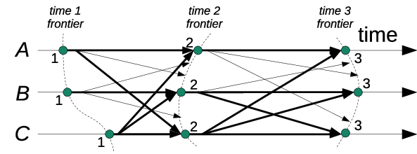
Figure 1 illustrates this process for a single three-node example with a message threshold . This TLC configuration requires each node to collect one other node’s step message in addition to its own before advancing and broadcasting its step message.
Different nodes may start at different real-world wall-clock times, and the network may arbitrarily delay or reorder the delivery of any node’s message to any other. This implies that different nodes may reach a given logical time-step at vastly different wall-clock times than other nodes. We refer to the varying sets of real-world times that different nodes arrive at a given logical step as the time frontier of step . Since each node advances its logical clock monotonically, the time frontier for each successive step divides real time into periods “before” and “after” step from the perspective of any given node . A given moment in real time may of course occur before from one node’s perspective but after for another node.
2.3 Causal Propagation of Messages
To simplify reasoning about logical time and the protocols we wish to build on it, we will assume that any TLC implementation ensures that knowledge propagates “virally” according to a causal ordering. For example, suppose node sends message at step , node receives it before moving to step and broadcasting message , and node in turn receives message . In this case, message is causally before . We will assume that the underlying network or overlay protocol, or the TLC implementation itself, ensures that node learns about message either before or at the same time as learns about : i.e., in causal order.
One way to ensure causal message propagation is conceptually trivial, if impractically inefficient. Each node simply includes in every message it sends a record of ’s entire causal history: e.g., a complete log of every message has ever received directly or heard about interactly from other nodes. There are more practical and efficient ways to ensure causally-ordered message delivery, of course: Section 9.3, will employ standard gossip and vector time techniques for this purpose. For now, we will simply take causally-ordered message propagation for granted as if it were a feature of the network.
2.4 Viral Advancement of Logical Time
A consequence of the threshold condition for time advancement, combined with causally-ordered message propagation, is that not just messages but also time advancement events propagate virally.
Suppose, for example, that node is waiting at logical time-step while another node has advanced to a later step arbitrarily far ahead of . If receives the message broadcast at step , then this delivery causes to “catch up” instantly to step . This is because, due to causal message propagation, obtains from not just ’s step broadcast but also, indirectly, the threshold set of messages used to advance from to , those that used to advance to , etc., up through step .
2.5 Information Propagation in TLC
The basic TLC protocol outlined above makes it easy to reason about the information that flowed into a node leading up to a particular time step . Because any node had to obtain a threshold of step messages, either directly or indirectly, in order to advance to at all, this trivially implies that ’s “view” of history at step will contain at least a fraction of all messages from step , as well as at all prior steps.
To build interesting protocols atop TLC, however, we will need to be able to reason similarly about information flowing out of a particular node into other nodes after some step . In particular, after a node broadcasts its step message, how can we tell how many nodes have received that message by some future logical time, say ? The adversarial network schedule ultimately determines this, of course, but it would be useful if we could at least measure after the fact the success (or lack thereof) of a given message’s propagation to other nodes. For this purpose, we enhance TLC to support witnessed operation.
2.6 Threshold Witnessed TLC
One way we can determine when a message broadcast by a node has reached other nodes is by requiring the node to collect delivery confirmations proactively, as a new prerequisite for the advancement of logical time. We might, for example, require each node to transmit each of its broadcasts to every other node and await TCP-like acknowledgments for its broadcast. If we require a node to confirm message delivery to all other nodes, or even to any pre-defined set of other nodes, however, this would present denial-of-service opportunities to the adversarial network, which could arbitrarily delay the critical message or acknowledgment deliveries.
To tolerate full network asynchrony, we must again invoke threshold logic, this time to confirm a message’s delivery to any subset of participants meeting some threshold, without caring which specific subset confirms delivery. Confirming message delivery to a threshold of participants is the basic purpose of a threshold witnessing protocol such as CoSi [155]. Threshold witnessing is useful, for example, in proactively ensuring the public transparency of software updates [68, 122] or building scalable cryptographically-trackable blockchains [92, 93, 90].
Threshold witnessing may be secured against Byzantine behavior using cryptographic multisignature or threshold signing schemes [56, 131, 147, 25, 58, 15]. Since we are assuming no Byzantine nodes for now, however, simple acknowledgments suffice for the moment in TLC.
We introduce a new witness threshold configuration parameter to TLC. A TLC protocol instance is thus now parameterized by message threshold , witness threshold , and total number of nodes . We will label such a TLC configuration for brevity. In practice we will typically pick either to be equal to , or to be zero, reducing to unwitnessed TLC as described above. We separate the message and witness thresholds, however, because they play orthogonal but complementary roles.

These threshold parameters establish a two-part condition for a node to advance logical time. To get from step to , each node must collect not just messages but threshold witnessed messages from step . Each threshold message must have been witnessed by at least participants before it can “count” towards .
To create a threshold witnessed message, each node first broadcasts its “bare” unwitnessed step message , and begins collecting witness acknowledgments on from participants serving as witnesses. Another node that receives in step simply replies with an acknowledgment that it has witnessed . Upon collecting a threshold of witness acknowledgments within step , node broadcasts an assertion that has been threshold witnessed. Only upon receiving this threshold witness confirmation may any node count towards its message threshold required to advance to step . Figure 2 illustrates this process in a simple 3-node configuration.
Suppose a node broadcasts an unwitnessed message for step , and another node receives not in step , but after having advanced to a later step . In this case, receiving node considers to be “too late” for step , and declines to witness for step . Instead, replies with the information needs to “catch up” to the most recent step that is aware of. If too many nodes receive ’s message too late, this may make it impossible for ever to be threshold witnessed – but can still advance its logical time with the information provided in lieu of a witness acknowledgment for step .
Due to network scheduling, a node may receive threshold witnessed messages of other nodes, and hence satisfy the conditions to advance time, before has obtained a threshold of witness acknowledgments to its own step message. In this case, simply abandons its collection of witness acknowledgments for its own message and moves on, using only other nodes’ threshold witnessed messages and not its own as its basis for advancing time. This rule preserves the property that time advancement advances virally, as discussed above, and ensures that a lagging node can “catch up” instantly to the rest upon receiving a message from a recent time-step.
With witnessed TLC, we now have a convenient basis for reasoning about information flow both into and out of a node at a given time-step. As before, we know that to reach step any node must have collected information – and hence be “caught up” on the histories of – at least nodes as of step . With witnessed TLC, we additionally know by construction that any node’s step message that is threshold witnessed by step has propagated “out” to and been seen by at least nodes by . Finally, because only threshold witnessed messages count towards the threshold to advance time, we know that by the time any node reaches step there are at least threshold witnessed messages from step .
2.7 Majoritarian Reasoning with TLC
So far we have developed TLC in terms of arbitrary thresholds and without regard to any specific choice of thresholds. But many interesting protocols, such as consensus protocols, rely on majoritarian logic: i.e., that a participant has received information from, or successfully delivered information to, a majority of participants.
For this reason, we now explore the important special case of TLC configured with majority thresholds: i.e., and . To tolerate Byzantine faults, Section 5 will adjust these thresholds to ensure majorities of correct, non-Byzantine nodes – but the fundamental principles remain the same.
Configured with majority thresholds, TLC offers two key useful properties: time period delineation and two-step broadcast. We develop these properties next.

2.8 Global time period delineation
Even though different TLC nodes reach a given time step at varying real times, majoritarian TLC nevertheless divides not just logical but also real wall-clock time into a well-defined quasi-synchronous succession of real time periods. The start of each global time period may be defined by the moment in real time that a majority of nodes first reaches a given logical time step . Figure 3 illustrates this principle, with real time delineated into successive time periods, each starting the moment the first two of the three nodes have advanced to a given time step.
Because each node’s logical clock advances monotonically, and a majority of nodes must reach step before a majority of nodes can reach , these majoritarian time periods likewise advance monotonically. These time periods in principle create the effect of a purely synchronous “lock-step” system, but with time periods “self-timed” by the progress of underlying network communication.
Even though these majoritarian time periods are easy to define in principle, we face a practical challenge in protocol design. Without precisely-calibrated real-time clocks, which we prefer not to assume, an individual node will rarely be able to tell whether it has advanced to logical time step before, or after, other participants. This implies in turn that no node can realistically be expected to know or determine precisely when a previous time period ends and the next begins. In the Figure 3 example, although globally there is a clear and well-defined “fact of the matter” regarding the moment each majoritarian time period begins and ends, a node will be unable to tell whether it advanced to step before majoritarian time period started (e.g., ), after period started (), or happened to be the “critical moment” that launched period ().
Despite this limitation in the knowledge of any given node, this majoritarian delineation of real time into periods gives us important tools for reasoning conservatively about when any particular message could, or could not, have been formulated and sent. Consider in particular a given time period , starting the moment a majority of participants reach step and ending the moment a majority of participants reach . We can be sure that:
- 1.
No node can advance to step , or send a message labeled , before the prior global time period has started. Such a node would have had to collect a majority of step messages to meet its condition to advance logical time, but no majority of step messages can be available to before a majority of nodes has actually reached step .
- 2.
After global time period has ended and begun, no node can formulate or successfully threshold witness any new message for step . Getting a step message threshold witnessed would require a majority of nodes to provide witness acknowledgments for step . But after period begins, a majority of nodes has “moved on” to and stopped providing witness acknowledgments for step , leaving only an inadequate minority of nodes that could potentially witness new messages for step .
Looking at an illustration like Figure 3, one might reasonably ask whether the wandering time frontiers, representing each node’s advancement to a given step , can “cross” over not only the majoritarian time period boundary, but also the time period boundaries before () and/or after (). The above two guarantees in a sense answer this question in the negative, effectively keeping all nodes approximately synchronized with each other, plus or minus at most one logical time step.
The first property above trivially ensures that no node can reach step 2 before global time period 1 has begun, can reach step 3 before period 2 has begun, etc. Thus, no node can “race ahead” of the majority’s notion of the current logical time by more than one time step.
And although communication patterns such as denial-of-service attacks could cause a particular node to “lag” many time-steps behind the majority in terms of real time, the second property above guarantees that such a lagging node cannot actually produce any effect, observable via threshold witnessed messages, after period has ended and begun. Any new messages the lagging node might produce after period has begun will effectively be “censored”, by virtue of being unable ever to be threshold witnessed. The lagging node will once again be able to send threshold witnessed messages when, and only when, it “catches up” to the current global time period.
2.9 Two-step semi-reliable broadcast
Another key property we obtain from majority message and witness thresholds is a guarantee that a majority of the messages sent at any time step will be known to all participants by step . TLC thus implicitly provides two-step broadcast at least for a majority, though not all, of the messages sent at any time step.
To see why this is the case, consider that in order for any node to advance to step , it must collect a majority of threshold witnessed messages from step . Each of these messages must have been seen by a majority of nodes in order to have been successfully threshold witnessed. To reach step , in turn, each node must collect a majority of threshold witnessed messages from step . The majority of nodes that witnessed any threshold witnessed message from step must overlap, by at least one node , with the majority of nodes that any other node collects messages from in order to reach . This intersection node effectively serves as a conduit through which is guaranteed to learn of message transitively through causal knowledge propagation, even if itself did not directly witness during step .
Since the real time at which nodes reach step is determined by the network’s arbitrary communication schedule, this two-step broadcast property can make no guarantees about when in real time any node actually learns about threshold witnessed message from step . A minority of nodes might lag many time steps behind the majority, and learn about only when they eventually “catch up” and resynchronize. By the time period delineation properties above, however, no lagging node will be able to have any effect on the majority, observable through threshold witnessed messages, before catching up with the majority. If the lagging node catches up at step or later, it learns about threshold witnessed message from step , through causal propagation, in the process of catching up.
It is important to keep in mind that this two-step broadcast property applies only to the “lucky” majority of messages that were threshold witnessed in step , however. A minority of messages that other participants tried to send in step may never be threshold witnessed before too many nodes advance to and the “gate closes” on step . These unlucky step messages might be seen by some participants, but TLC can make no guarantee that all, or any particular number, of participants will ever see them. Further, the adversarial network gets to decide which messages are in the lucky majority that are threshold witnessed and broadcast, and which are unlucky and potentially lost to history. Messages that fail to achieve threshold witnessed status during a time step may be considered casualties of network asynchrony.
Another subtle but important caveat with two-step broadcast in TLC is that even if message is threshold witnessed in step and broadcast to all nodes by , this does not mean that all nodes will know that was threshold witnessed by . Suppose a node receives and acknowledges the bare, unwitnessed version of during step , for example, thereby contributing to the eventual threshold witnessing of . Node might then, however, advance to steps and on the basis of other sets of threshold witnessed messages not including , without ever learning that was fully threshold witnessed. In this case, while has indeed, like all nodes, seen at least a bare unwitnessed version of by step , only some nodes may know by that was successfully threshold witnessed. This subtlety will become important later in Section 4.5 as we build consensus protocols atop TLC.
3 Building Basic Services on TLC
Before we tackle asynchronous consensus in Section 4, we first briefly sketch several classic distributed services not requiring consensus that are easy and natural to build using TLC for pacing. While these services may of course be built without TLC, the threshold logical clock abstraction makes it simple for such distributed services to operate atop fully asynchronous networks in self-timed fashion as quickly as network communication permits.
3.1 Network Time Services
Even in asynchronous distributed systems that we do not wish to be driven by wall-clock time or timeouts, it is still important in many ways to be able to tell time and interact properly with the wall clock. We first discuss three basic time-centric services and how they might benefit from asynchronous operation atop TLC: clock synchronization, trusted timestamping, and encrypted time capsules.
3.1.1 Clock Initialization and Synchronization
Time services such as NTP [118, 117], by which networked devices around the world synchronize their clocks, play a fundamental role in the Internet’s architecture. Without time services, all devices’ real-time clocks gradually drift, and can become wildly inaccurate after power or clock failures. Drifting or inaccurate device clocks can undermine the functioning of real-time systems [94] and wireless sensor networks [167, 153]. Security protocols often rely on devices having roughly-synchronized clocks [54, 159, 158], otherwise becoming vulnerable to attacks such as the replay of expired credentials, certificates, or outdated software with known exploits [122].
While a correct sense of time is critical to the reliability and security of today’s networked devices, numerous weaknesses have been found in traditional time services [139, 71, 110, 111, 112]. The fact that clients typically rely entirely on a single NTP time server (e.g., the nearest found on a list) is itself an inherent single-point-of-failure weakness. Using GPS as a time source [101, 51], while ubiquitous and accurate under normal conditions, is less trustworthy as GPS spoofing proliferates [129, 137, 30]. A networked device might achieve a more secure notion of the time by relying on a group of independent time servers rather than just one, thereby avoiding any single point of failure or compromise.
TLC represents a natural substrate atop which to build such a distributed time service or beacon. One simple approach is for each each server in a TLC coordination group to publish a log (or “blockchain”) of current-time records, one per TLC time-step. Each successive record indicates the server’s notion of the record’s publication time, ideally measured from a local high-precision source such as an atomic clock. Each published record is both digitally signed by the server, and witness cosigned by other coordination group members [155], thereby attesting to clients jointly that the server’s notion of time is consistent to some tolerance. Clients may still follow just one time server at a time as they currently do (e.g., the closest one), but protect themselves from major inaccuracy or compromise of their time source by verifying the witness cosignatures as well. We address later in Section 9.3 the important detail of allowing witnesses to validate proposed time records in an asynchronous setting without introducing arbitrary timeouts or tolerance windows.
The precision a distributed time beacon can provide will naturally depend on factors such as how widely-distributed the participating servers are and how reliable and predictable their mutual connectivity is. Building a distributed time beacon atop TLC offers the potential key benefit of adapting automatically to group configurations and network conditions. A time beacon composed of globally-distributed servers could offer maximum independence and diversity, and hence security, at the cost of limited precision due to the hundreds-of-milliseconds round-trip delays between group members. Such a widely-distributed service could offer client devices a coarse-grained but highly-secure “backstop” reference clock ensuring that the device’s clock cannot be off by minutes or hours even if more-precise time sources are unavailable or subverted. Another complementary time beacon running the same TLC-based protocol, but composed of servers colocated in a single city or data center with a low-latency interconnect, would automatically generate much more frequent, high-precision time reports, while still avoiding single points of failure and degrading gracefully during partial failures or attacks.
3.1.2 Trusted Timestamping and Notarization
A closely-related application is a digital timestamping service, which not only tells the current time, but also produces timestamps on demand attesting that some data known to the client existed at a certain time. Standards such as the Time-Stamp Protocol [4, 5] allow clients to request a signed timestamp on cryptographically hashed data from a trusted timestamping authority. Such an authority is again a single point of failure, however, motivating recently-popular decentralized approaches to timestamping, such as collecting content hashes into a Merkle tree [115] and embedding its root in a Bitcoin transaction [121, 156], or collectively signing each root [155].
An asynchronous distributed timestamping service, whose period and timestamp granularity is self-timed to the best allowed by group configuration and prevailing network conditions, represents a natural extension to a TLC-based time service. Each server in such a group might independently collect client-submitted content hashes into Merkle trees, publishing a signed and witness cosigned tree each TLC time step, as in the CoSi time service [155, Section V.A]. In addition, a newly-started or long-offline device can bootstrap its internal clock with strong freshness protection, preventing an upstream network attacker from back-dating its notion of time, by initializing its clock according to a witness cosigned timestamp it requests on a freshly-generated random nonce.
3.1.3 Encrypted Time Capsules
A third classic time-related service with many potential uses is a cryptographic time vault or time capsule, allowing clients to encrypt data so that it will become decryptable at a designated future time. In games, auctions, and many other market systems, for example, participants often wish to encrypt their moves or bids from others until a designated closing time to guard against front running [50, 61]. Time-lock puzzles [136] and verifiable delay functions [24, 162] represent purely cryptographic proposals to achieve this goal, but cryptographic approaches face inherent challenges in accurately estimating the future evolution of, and market investment in, computational and cryptanalytic puzzle-solving power [108, 45].
Another approach to time capsules more compatible with TLC relies on a time service that holds a master key for identity-based encryption (IBE) [146, 26, 160]. Clients encrypt their messages to a virtual “identity” representing a particular future time. The time service regularly generates and publishes the IBE private keys representing these “time identities” as they pass, allowing anyone to decrypt any time-locked ciphertext after the designated time passes. Threshold secret-sharing [145, 152, 144] the IBE master key among the group avoids single points of failure or compromise. The asynchronous setting presents the challenge that clients seemingly must predict the future rate at which the time capsule service will operate, and hence the granularity at which it will publish time-identity keys, a detail we address later in Section 9.3.
3.2 Public Randomness Beacons
Like time, trustworthy public randomness has become an essential “utility” needed by numerous applications. Lotteries and games need random choices that all participants can trust to be fair and unbiased, despite the many times such trust has been breached in the past [64, 161, 149, 69]. Governments need public randomness to choose a sample of ballots to select jury candidates [138], to audit election results [35, 104], and experimentally, to involve citizens in policy deliberation through sortition [67, 57]. Large-scale decentralized systems such as blockchains need public randomness to “scale out” via sharding [106, 93].
The many uses for public randomness have inspired beacons such as NIST’s [89]. Concerns about centralized beacons being a single point of compromise [151], however, again motivate more decentralized approaches to public randomness [33, 42, 100, 27, 154]. Threshold-secure approaches [33, 154, 96] are naturally suited to being built on TLC, which can pace the beacon to produce fresh random outputs dynamically as often as network connectivity permits, rather than at a fixed period.
4 Que Sera Consensus (QSC)
We now explore approaches to build consensus protocols atop TLC, using a series of strawman examples to address the key challenges in a step-by-step fashion for clarity. This series of refinements will lead us to QSC3, a randomized non-Byzantine (i.e., Paxos-equivalent) consensus protocol. We leave Byzantine consensus to Section 5.
Although the final QSC3 protocol this section arrives at is quite simple, the reasoning required to understand and justify it subtle, as with any consensus protocol. A desire to clarify this reasoning motivates our extended, step-by-step exposition. Expert readers may feel free to skip to the final solution summarized in Section 4.10 if desired.
4.1 Strawman 0: multiple possible histories
As a starting point, we will not even try to achieve consensus reliably on a single common history, but instead simply allow each node to define and build its own idea of a possible history, independently of all other nodes. For convenience and familiarity, we will represent each node’s possible history as a blockchain, or tamper-evident log [143, 49] in the form popularized by Bitcoin [121].
At TLC time-step 0, we assume all nodes start building from a common genesis block that was somehow agreed upon manually. At each subsequent time-step, each node independently formulates and proposes a new block, which contains a cryptographic hash or back-link to the previous block. Thus, node ’s block 1 contains a hash of the genesis block, node ’s block 2 contains a hash of node ’s block 1, and so on. The main useful property of this structure is that the blockchain’s entire history is identified and committed by knowledge of the head, or most recent block added. It is cryptographically infeasible to modify any part of history without scrambling all the hash-links in all subsequent blocks including the head, thereby making any modification readily detectable.

Figure 4 illustrates three nodes building three independent blockchains in this way. The real (wall-clock) time at which each node reaches a given TLC time-step and proposes the corresponding block on its blockchain may vary widely across nodes due to network delays, but TLC serves to pace all nodes’ advancement of time and keep them logically in lock-step despite these delays.
If we assume each node’s proposed block at a given time-step contains a set of transactions submitted by clients, as in Bitcoin, then even this strawman protocol can provide a limited notion of “consensus.” If a client submits some transaction to all nodes (e.g., “Alice pays Bob 1 BTC”), and the client succeeds in getting embedded in each node’s history, then the client can consider to be “committed.” This is because regardless of which of the posssible histories we might choose to believe, all of them contain and account for transaction .
However, if a “double-spending” client manages to get onto some nodes’ blockchains and gets a conflicting transaction onto others (e.g., Alice pays Charlie the same 1 BTC), then we will forever be uncertain whether Bob or Charlie now holds the 1 BTC and unable ever to resolve the situation. Thus, we need a way to break the symmetry and enable some competing histories to “win” and others “lose” – the challenge we tackle next.
4.2 Strawman 1: genetic consensus
Introducing randomness makes it surprisingly simple to create a working, if non-ideal, consensus protocol. Suppose we modify the above strawman such that at each time-step, one randomly-chosen node chooses to adopt and build on the blockchain of a randomly-chosen neighbor instead of its own. This node’s prior history is thus dropped from the space of possibilities, and effectively replaced with the node’s newly-adopted view of history.

Consider the simple example in Figure 5. At TLC step 1, each node independently builds on the genesis block as before. At step 2, however, node randomly chooses to build on ’s prior blockchain instead of its own. Similarly, at step 3, node chooses to adopt ’s blockchain. While we still have three competing heads and hence competing histories (namely , , and ), nevertheless they happen to share a common prefix, namely block . Because all future time-steps must build on one of these three possible histories, all sharing this common prefix, we can consider the common prefix (block ) to be committed – even if we can’t (yet) say anything about the more recent blocks. This situation is directly analogous to the common event of a temporary fork in Bitcoin, where two miners mine competing blocks at about the same time, deferring resolution of the conflit for later. The main difference is that we pace the “mining” of blocks in our protocol using TLC instead of via proof-of-work.
Whenever one node adopts another’s blockchain, any transactions that had existed only in the node’s prior blockchain become lost or in effect “aborted.” All transactions on the adopted blockchain, in contrast, become more likely to survive long-term because they are represented redundantly in the (new) history of one additional node, and become correspondingly more likely to propagate further via future adoption events. If we ever happen to observe that through this random history-adoption process, a particular transaction of interest has propagated to all nodes’ view of history, then we can consider that transaction to be definitely “committed.” But will every transaction reach such a state of being definitely either “committed” (by virtue of being on all nodes’ views of history) or “aborted” (by virtue of being on none of them)?
Given time, the answer is definitely yes. This is because from the perspective of a particular transaction that any node first introduces in a block on its local blockchain, that transaction’s subsequent propagation or elimination corresponds to a Moran process [119, 123], a statistical process designed to model genetic drift in a population constrained to a fixed size (e.g., by natural resource limits). A node’s adoption of another’s blockchain corresponds to the successful “reproduction” of the adopted blockchain, coincident with the “death” of the replaced blockchain. We might view all the transactions in the adopted blockchain’s view of history to be the “genome” of the successfully-reproducing blockchain, whose constituent blocks and transactions become more likely to survive with each successful reproduction.
This process is a variation on the Pólya urn model [86, 109, 128], where we view each competing blockchain (or the transactions on them) as colored balls in an urn. From this perspective, we view one node’s adoption of another’s blockchain as the removal of a pair of colored balls from the urn, where we duplicate one, discard the other, and return the two duplicates to the urn. With time, this process guarantees that any particular transaction in any particular blockchain’s “genome” is eventually either lost (aborted) or propagated to all other individuals (committed). If all nodes’ blockchains have the same “genetic fitness” or likeliness to reproduce, then a transaction first introduced in a block on any one node has a uniform probability of of eventually being “committed” this way.
Of course, this strawman has several obvious limitations. is not a great probability of a proposed transaction being successfully committed. We must wait a considerable time before we can know a transaction’s commit/abort status for certain. And we must monitor all nodes’ blockchains – not just a threshold number of them – in order to reach absolute certainty of this commit/abort status. However, this strawman does illustrate how simple it can be in principle to achieve some notion of “consensus” through a simple random process.
4.3 Strawman 2: a genetic fitness lottery
We can speed up the above “genetic process” in two ways, which we do now. First, we can simply increase the global rate of death and reproduction, by requiring several – even all – nodes to replace their history at each time-step with a randomly-chosen node’s prior history. TLC’s lock-step notion of logical time facilitates this process. At each step each node proposes and announces a new block, then at each node chooses any node’s step block at random to build on in its step ’s proposal. Thus, each node’s proposal will survive even just one round only if some node (any node) happens to choose it to build on.
The second, more powerful way we can accelerate the process – and even achieve “near-instant” genetic consensus – is by using randomness also to break the symmetry of each proposal’s “genetic fitness” or likeliness to reproduce. At each TLC time-step , each node announces not only its newly-proposed block, but also chooses and attaches to its proposal a random numeric lottery ticket, which will represent the proposal’s “genetic fitness” relative to others. These lottery tickets may be chosen from essentially any distribution, provided all nodes correctly choose them at random from the same distribution: e.g., real numbers between 0 and 1 will work fine.
By TLC’s progress rules, each node must have collected a threshold number of proposals from step as its condition to progress to step . Instead of picking an arbitrary one of these proposals to build on in the next consensus round starting at , each node must now choose the step proposal with the highest-numbered lottery ticket that knows about: i.e., the most “genetically fit” or “attractive” proposal it sees. Step proposals with higher fitness will be much more likely to “survive” and be built upon in subsequent rounds, while proposals with lower fitness usually disappear immediately because no one chooses to build on them in subsequent rounds.

Figure 6 illustrates this process. At step 2, all three nodes see and thus choose node ’s “maximally fit” proposal from step 1 to adopt and build on, thereby achieving instant commitment globally. At step 3, however, nodes and choose the second-most-fit proposal by , because ’s globally-winning proposal was unfortunately not among those that or collected in progressing to TLC step 3. With global knowledge, at step 3 we can be certain that all transactions up through block are committed, but we remain uncertain whether blocks or will eventually win since both still survive at step 3.
If all nodes correctly follow this process, then we reduce the number of possible blockchains effectively surviving and emerging from any time period from down to . This is because when any node reaches step , there are at most proposals it might have missed seeing upon meeting the threshold condition to reach , and hence at most proposals might have had a better fitness than the best proposal saw and picked. While reducing the possibility space from possible histories to represents an improvement, it is still far from our goal of course – but we are moving in the right direction.
4.4 Strawman 3: a contest of celebrities
While we have accelerated genetic consensus and reduced the number of possible histories that can survive at each step, we still face the problem that no one can be certain whether consensus has actually been achieved without seeing all nodes’ choices at each time-step. If any node, or one of their clients, tried to collect this information globally, it might hang waiting to hear from one last long-delayed or failed node, defeating the high-availability goal of threshold coordination. It thus appears we can never discern consensus with certainty.
In Figure 6, for example, node may be unable to distinguish between the “consensus” situation at step 2 and the “lack of consensus” situation at step 3, if has seen only ’s step 2 decision and not ’s upon reaching step 3. cannot just wait to hear from as well without compromising availability, but also cannot exclude the risk that a higher-fitness “minority opinion” such as block might exist and eventually win over those knew about.
This “minority report” problem suggests an appealing solution: let us restrict the genetic competition at each step only to celebrity proposals, or those that a majority of nodes have heard of by the next time-step when it is time to pick winners. By having each node choose the most fit only among celebrity proposals, we hope to prevent an unknown, high-fitness, “dark horse” from later “spoiling” what might appear to be consensus. This attempt will fail, but in a useful way that moves us toward a solution.
TLC’s threshold witnessing process in each round conveniently provides information useful to identify celebrity proposals. We will say that participant confirms proposal as a celebrity proposal if was among the set of threshold-witnessed messages used to advance its logical clock to step . Since each participant must collect a threshold number of threshold-witnessed messages from step in order to transition to step , each node automatically confirms a majority of proposals by .
We now require that each participant choose its best confirmed proposal, having the highest-numbered lottery ticket, as its “preferred” step proposal to build on at step . Step proposals not in node ’s threshold witnessed set – i.e., the at most proposals that did not wait to be confirmed before moved to – are thus not eligible from ’s perspective to build on at .
With this added rule, each proposal from step that survives to be built on at , is, by protocol construction, a proposal that most of the participants (all but at most ) have seen by step . Intuitively, this should increase the chance that “most” nodes at will choose and build on the same “lottery winner” from step . This rule still leaves uncertainty, however, since different participants might have seen different subsets of confirmed proposals from step , and not all of them might have seen the eligible proposal with the globally winning ticket.
4.5 Strawman 4: seeking universal celebrity
To address this lingering challenge, it would seem useful if we could be certain that not just a majority of nodes, but all nodes, know about any proposal we might see as a candidate for achieving consensus. Further refining the above celebrity approach, in fact, we can ensure that celebrity proposals known to a majority of nodes reach universal celebrity status – becoming universally known to all participants – simply by “biding our time” for a second TLC time-step during each consensus round.
Recall from Section 2.9 that with majority thresholds, any message that is broadcast at time-step and is threshold-witnessed by step will have propagated to all nodes by step . This is because the set of nodes that witnessed by step must overlap by at least one node with the set of nodes whose step messages any node must collect in order to reach step .
Motivated by this observation, we now modify the consensus process so that each round requires two TLC time-steps instead of one. That is, each consensus round will start at step , and will finish at step , the same logical time that consensus round starts.
At step , each node proposes a block as before, but waits until step to choose a step proposal to build on in the next consensus round. Because the universal broadcast property above holds only for messages that were witnessed by a majority of nodes by step , we must still restrict each node’s choice of proposals at step to those that had achieved majority celebrity status by step . Among these, each node as usual chooses the eligible proposal from step with the highest lottery ticket.

By slowing down consensus, we ensure the promising property that whichever step proposal a node might choose for the next round at , all nodes know about proposal by step . Figure 7 illustrates this process in a scenario in which ’s proposal at step is threshold witnessed by nodes by step to achieve celebrity status, then as a result propagates to all nodes by .
Are we done? Unfortunately not. As discussed earlier in Section 2.9, the fact that all nodes know the existence of by step does not imply that all nodes will know the crucial fact that was threshold witnessed, or thus have confirmed as having celebrity status by .
Due to message timing, different nodes may reach steps and on the basis of different subsets of threshold-witnessed messages. For example, one node might see that proposal was threshold-witnessed by step , and eventually choose it as the best eligible proposal by . Another node , in contrast, might have reached step on the basis of a different set of witnessed messages than used. If proposal isn’t in ’s threshold-witnessed set by , cannot “wait around” to see if eventually becomes fully threshold-witnessed without compromising ’s availability, so must move on.

In this case, will definitely learn the existence of proposal by step , from at least one of the majority set of nodes that witnessed by . But this fact tells only that at least one node witnessed , not that a majority of nodes witnessed by , as required for to confirm as eligible for the next round to build on. In this situation, nodes and may pick different eligible proposals to build on in the next round, and neither nor has any readily-apparent way to distinguish this consensus failure situation from one in which all nodes fortuitously do choose the same best eligible proposal. Figure 8 illustrates such a failure case, where the globally best proposal is threshold witnessed by but only node actually learns by then that proposal is eligible.
4.6 Strawman 5: enter the paparazzi
Is there some way a node can tell not only that a proposal has reached celebrity status by and thus that ’s existence will be known to all nodes by , but additionally that the fact of ’s celebrity status will also become known to all nodes? We can, by a second application of the same two-step broadcast principle, merely shifted one time-step later. Suppose a node confirms ’s celebrity status at step , then successfully “gossips” that fact to a majority of nodes by . Then not only the existence of but also ’s confirmation of ’s celebrity status will subsequently become known to all nodes by .
We therefore extend each consensus round to take three TLC time-steps, so that round starts at step and ends at . In addition, we will try to strengthen the eligibility criteria for proposals to ensure that both the existence and the celebrity status of any chosen proposal becomes known to all nodes by . In particular, for any node to consider a proposal broadcast at to be eligible for the consensus round’s genetic lottery, must see that: (a) some node , who we’ll call the paparazzi, observed and reported ’s celebrity status in ’s broadcast at step ; and (b) that ’s broadcast at was in turn threshold witnessed by a majority of nodes by step .

For brevity, we will say that the paparazzi node first confirms proposal ’s celebrity status at step , then in turn confirms ’s step broadcast in the same way. When such a “double-confirmation” linked by paparazzi node occurs, we say that node reconfirms proposal . Node ’s confirmation of at ensures that all nodes will know the existence of by , and ’s reconfirmation of at in turn ensures that all nodes will know of ’s confirmation of by . Figure 9 illustrates this process, with node acting as paparazzi for ’s proposal in an example 3-step consensus round.
Are we done yet? Unfortunately we’ve merely kicked the can down the road. If node reconfirms by step , this implies that all nodes will know by that was confirmed, but it does not imply that other nodes will have reconfirmed . If reconfirmation and not just confirmation is ’s new eligibility condition, then we must account for the fact that we have moved the goalposts. By the end of the round at , different nodes may still disagree on whether was reconfirmed and hence (still) eligible for the genetic lottery, once again allowing disagreement about the consensus round’s result in the end.
We could try playing the status gossip and confirmation game yet again, making triple-confirmation the proposal eligibility condition, but this approach just leads us in circles. A proposal’s triple-confirmed status will ensure that all nodes know by that it was double-confirmed, but will still leave disagreement on whether it was triple-confirmed. We must therefore try something else: it is hard to win a game of counting to infinity.
4.7 Strawman 6: gazing into the crystal ball
Since we would appear to need an infinite amount of time to get “complete” information about a consensus round, let us instead make the best we can of incomplete information. We will therefore return to using only (single) confirmation as the eligibility criterion for a proposal to enter the genetic lottery. We will then use (double) reconfirmation to give us an unreliable “crystal ball” that sometimes – when we’re lucky – enables some nodes to predict when all other nodes will just happen to converge and agree on the same “best eligible proposal” during the round.
Our crystal ball will sometimes be clear, allowing a precise prediction, and sometimes cloudy, offering no useful information. Further, the crystal ball may appear clear from the perspective of some nodes, and cloudy to others, even in the same consensus round. The crystal ball’s subjective fickleness may therefore leave only some nodes aware when consensus succeeds, while other nodes must wait until future rounds to learn this fact in retrospect.
Since all nodes are again using (single) confirmation as their criterion for a proposal ’s eligibility, this implies that no node will choose in this round unless at least the existence of proposal (though not necessarily its celebrity status) has become known to all nodes by step . Now suppose that some node happens to notice that is not just confirmed but is in fact reconfirmed (double-confirmed) by step . This does not tell that other nodes will also reconfirm , but it does tell that all other nodes will have at least (singly) confirmed by step . Thus, node knows – even if other nodes don’t – that all nodes will realize by that is eligible.
Finally, suppose that by step , node is also not aware of the existence of any other proposal , confirmed or not, having a lottery ticket competitive with that of (i.e., a value greater than or equal to ’s ticket). Since any such competitive proposal cannot become eligible, or be confirmed by any node, without at least ’s existence becoming known to all nodes by , the fact that has not seen any sign of a competitive proposal implies that there can be no eligible competitor to . There could be proposal with a competitive ticket value that didn’t see, but to be “hidden” from in this fashion, must have been seen by only a minority of nodes, and thus cannot be eligible and cannot have been confirmed by anyone.
Since now knows from ’s reconfirmation that all nodes will know and have confirmed by , and no other eligible proposal competitive with exists that any node could confirm to spoil ’s victory, this means that has successfully “gazed into the crystal ball” and predicted this round’s inevitable convergence on . Node can predict with certainty that all nodes will choose as their best eligible proposal to build in the next round, even though these other nodes themselves may not be aware of this convergence. Since all future histories must now build on , can consider all transactions in and all prior blocks that built on to be permanently committed.
Since other nodes may not obtain the same information as in this round, other nodes may see the crystal ball as cloudy, and be forced to assume conservatively that consensus may have failed, and that different nodes might pick different best eligible proposals. These other nodes will eventually learn, in some future round in which they successfully use the crystal ball, that has been committed as a prefix to some longer history that has by then been built atop proposal . The fact that only some nodes (or even no nodes) might actually know in this round that all nodes have converged on does not change the inevitably – or “fate” – that all future history will build on .
Some consensus rounds may also genuinely fail to converge, in which case different nodes see and choose different proposals as the best eligible. In this case, all nodes will perceive the crystal ball as cloudy. Some nodes might fail to discern the eligibility status of the best (globally) eligible proposal, instead seeing that proposal as a “spoiler” competitive with some next-best proposal that they do confirm as eligible. Other nodes might confirm the best proposal as eligible, but fail to reconfirm it because knowledge of the proposal’s eligibility failed to propagate to a majority of nodes, making the proposal’s reconfirmation impossible. In any case, any consensus round that fails to converge can still safely yield multiple “competing” proposals, as in earlier cases above, to be left for resolution by a more-fortunate future consensus round.
4.8 Something wicked this way routes
Having resigned ourselves to the possibility that only some consensus rounds may succeed, and that only some nodes may even realize that a round succeeded, we would like to know whether and how often we can actually anticipate this desirable outcome. If the network is truly adversarial, however, choosing message delays and delivery orders intelligently to prevent consensus from succeeding, for example, then we still appear to have a problem.
If the adversary can see the lottery ticket for each proposal as soon as is broadcast at a consensus round’s start time , the adversary can arrange message delivery order so that no consensus round ever succeeds. For example, the adversary can first collect all proposals from step along with their lottery tickets, then arrange for the proposals with the three highest-valued lottery tickets each to be witnessed by only a third of the nodes each, ensuring that none of these proposals propagate to a majority of nodes by step to become eligible. Any other proposal that any node might confirm as eligible will always be “spoiled” by one of the best three (always-ineligible) proposals, preventing convergence and keeping all nodes’ crystal balls permanently cloudy.
We could just assume that the network schedules message deliveries arbitrarily but obliviously to the values computed and used in distributed protocols, as in oblivious scheduler models [11, 12, 8, 70, 9]. In today’s open Internet, however, the threat of intelligent disruption from network adversaries is unfortunately all too realistic.
Fortunately, we have a conceptually simple way to ensure that the adversary cannot interfere with consensus in this fashion. We simply ensure that the adversary cannot know the lottery tickets associated with each proposal until later, after the consensus round has completed and the adversary has already “committed” its decisions on network delays and ordering. In effect, if we force the network adversary to “play its hand” first, by forwarding enough messages to allow the consensus round to complete before the adversary can learn any lottery ticket values, then we can ensure by design that the adversary’s decisions are independent of the lottery tickets – exactly as if network ordering was arbitrary but oblivious.
How can we ensure that an adversarial network does not learn the proposals’ lottery ticket values before the consensus round completes? In the present non-Byzantine case in which we assume all nodes are correct, we can rely on them not to leak information to the network adversary directly. We therefore need only to ensure that ticket values do not leak to the network adversary while in transit over the network, which we can accomplish simply by encrypting the lottery ticket values – or better yet in practice, all inter-node communication – using a standard pairwise encryption protocol such as TLS [135]. This approach obviously fails as soon as there is even one Byzantine node that might leak the lottery ticket values to the adversary; we address this problem later in Section 5 using Shamir secret sharing [145, 152, 144]. For now, however, we simply assume that the lottery ticket values are kept out of the adversary’s knowledge “somehow” until the consensus round is over, so that we can assume that they are independent of network delays and ordering considerations.
4.9 Calculating the odds of success
Given that lottery ticket values are independent of network scheduling, we can now analyze the probability that any particular node will “get lucky” and observe a consensus round to succeed. This occurs only when all nodes converge on the same proposal , and node in particular is able to detect this convergence by reconfirming (double-confirming) proposal . We focus this analysis purely on what a particular node observes, because we merely want to ensure that each node observes success “often enough” regardless of any other node’s experience.
For simplicity, we will conservatively focus our analysis on the event that observes the globally highest-numbered proposal to commit. This situation is sufficient, but not necessary, for to observe success. Network scheduling could cause all nodes to converge on a proposal other than the global best, and cause to witness this as successful commitment, if any other higher-numbered proposals do not become eligible and fail to arrive at to “spoil” its view. But this (likely rare) event can only improve ’s observed success rate, so we ignore it and focus only on commitments of the globally-best proposal.
Recall the two key conditions above for to see in its “crystal ball” that proposal has been committed: (a) that has reconfirmed , and (b) that has seen no other proposal from step , confirmed or not, with a lottery ticket value competitive with ’s. By our assumption that is the globally-best proposal, (b) cannot happen since no proposal globally better than exists. We also assume here that lottery tickets have enough entropy that the chance of a tie is negligible, but accounting for ties of known probability requires only a minor adjustment to the analysis.
We therefore care only about the probability that reconfirms : i.e., that some paparazzi node confirms at step and subsequently confirms ’s step confirmation of . Recall that had to collect threshold-witnessed messages from a majority of nodes to reach step . If any one of these nodes has confirmed by , then will subsequently confirm ’s confirmation and hence reconfirm . The probability that at least one of these potential paparazzi confirms is no less than the probability that any particular one does, so we can again focus conservatively on some particular node .
Node , in turn, had to collect threshold-witnessed proposals from a majority of nodes in order to reach step . If any one of these proposals is the proposal with the globally highest ticket, then will certainly confirm at . Since each of the nodes’ proposals have a chance of being the globally highest, and this is unpredictable to the network adversary, the chance of node observing any given round to succeed is at least .
Although the probabilities that different nodes in the same round observe success are interdependent in complex ways, the probabilities of observing success across successive rounds is independent because each round uses fresh lottery tickets. The success rate any node observes therefore follows the binomial distribution across multiple rounds. The probability that a node fails to observe a successful commitment in consecutive time steps is less than , diminishing exponentially as increases.
4.10 Summary: whatever will be, will be
In summary, we have defined a simple randomized consensus protocol atop majority-witnessed TLC. In each consensus round starting at TLC time step , each node simply proposes a block with a random lottery ticket, waits three TLC time-steps, then uses the communication history that TLC records and gossips to determine the round’s outcome from any node’s perspective.
In particular, each node always chooses a best confirmed proposal from round to build on in the next round . Node confirms a proposal sent in step if can determine that was threshold-witnessed by a majority of nodes by step . A best confirmed proposal for is any round proposal has confirmed whose lottery ticket is greater than or equal to that of any other proposal has confirmed in this round.
In addition, node decides that the consensus round has successfully and permanently committed proposal if all of the following three conditions hold:
- •
Node obtains a step message , from some node , that can confirm was threshold-witnessed by a majority of nodes by ;
- •
Node ’s message at recorded that proposal from step was threshold-witnessed by a majority of nodes by ; and
- •
No other step proposal that has become aware of by step has a lottery ticket greater than or equal to that of .
Each node will observe successful consensus in this fashion with an probability of at least in each round, independently of other rounds. Any round that sees as successful permanently commits both proposal and any prior uncommitted blocks that built on. Thus, the probability has not yet finalized a unique proposal for round by a later round for is at most .
4.11 Optimizing performance: pipelining
For simplicity we have described QSC with rounds running sequentially, each round starting at TLC time-step and ending at step . A simple optimization, however, is to pipeline QSC consensus rounds so that a round starts on every time-step and overlaps with other rounds. With pipelining, each consensus round starts at step and ends at step . In this way, we can smooth the communication and computation workload on nodes at each timestep, minimize the time clients submitting transactions have to wait for the start of the next consensus round, and reduce the average time clients must wait for a transaction to commit, since commitment occurs with constant probability for each completed round and pipelining triples the rate at which rounds complete.
One apparent technical challenge with pipelining is that at the start of round (step ), when each node broadcasts its proposal, we might expect this proposal to include a new block in a blockchain. To produce a blockchain’s tamper-evident log structure [143, 49], however, each block must contain a cryptographic hash of the previous block. But the content of the previous block is not and cannot be known until the prior consensus round ends at step , which due to pipelining is two time-steps after step , when we appear to need it!
The solution to this challenge is to produce complete blocks, including cryptographic back-links, not at the start of each round but at the end. At the start of round (step ), each node broadcasts in its proposal only the lottery ticket and the semantic content to be included in this block, e.g., a batch of raw transactions that clients have asked to commit. Only at the end of round , at step , do nodes actually form a complete block based on this proposal. All nodes, not just the original proposer, can independently compute the block produced by round ’s winning proposer, deterministically based on the content of its step proposal and the block it builds on from the previous round , which we now know because it was fully determined in step .
A second-order challenge that this solution creates is that in transactional systems, the proposer of a block cannot necessarily know for sure at proposal time that all of the transactions it is proposing will still be committable by the completion of the consensus round. For example, at the start of consensus round , a node might propose a batch of transactions including the payment of a coin from Alice to Bob. Alice might indeed own the coin to be spent according to node ’s view of the blockchain at step – but by the end of round , at step , the coin might have already been spent in a conflicting transaction appearing in the blocks is building on from the rounds completing at steps and . The deterministic block-formation function that all nodes run at the end of each round can account for this risk simply by discarding such transactions that have become uncommittable by the time they were proposed, leaving them out of the block produced at step without blaming the block’s proposer for an event it could not have forseen.
5 Tolerating Byzantine Nodes
For simplicity we have assumed so far that only the network, and not the participating nodes themselves, might exhibit adversarial behavior. Both TLC and QSC may be extended to tolerate Byzantine behavior using well-known existing techniques, however, as we outline in this section. We address this challenge in three main steps, roughly corresponding to three key layers of functionality from bottom to top: first, enforcing the causal ordering that TLC depends on; second, ensuring TLC’s correct time progress in the presence of Byzantine nodes; and third, protecting QSC consensus from adversarial nodes.
5.1 Causal Logging and Accountability
While TLC’s goal is to create a “lock-step” notion of logical time, to build TLC and secure it against Byzantine nodes, it is useful to leverage the classic notion of vector time [66, 105, 114, 63] and associated techniques such as tamper-evident logging [143, 49], timeline entanglement [113], and accountable state machines [79, 78].
5.1.1 Logging and Vector Time
Our approach hinges on transparency and accountability through logging and verification of all nodes’ state and actions. Each node maintains a sequential log of every significant action it takes, such as broadcasting a message. Each node’s log also documents the nondeterministic inputs, such as messages it received, that led it to take that action. Each node assigns consecutive sequence numbers to its log entries. A node’s sequence numbers effectively serve as a node-local logical clock that simply counts all the events the node records, independent of both wall-clock time and other nodes’ sequence numbers.
In addition to logging its own events, each node also maintains a mirror copy of all other participating nodes’ logs, and continuously tracks their progress by maintaining a vector containing the highest sequence number has seen so far from each other node . This is the essence of the classic concept of vector clocks [114, 63].
Because a vector clock indicates only that some node has seen all the logged events of some other node up to a particular sequence number in ’s local sequence space, node must process messages from , and update its vector clock accordingly, strictly in the order of ’s sequence numbers. Suppose has seen all messages from up to sequence number , for example, then receives a message containing ’s event out of order. In this case, must hold this out-of-order message in a reordering buffer and delay its actual processing and internal delivery until receives a message from filling in the missing sequence number 4. This reordering process is no different from classic in-order delivery protocols such as TCP [157].
Whenever node records a new entry in its log, it includes in the new entry a vector timestamp, which documents, for the benefit and validation of other nodes, which messages from all nodes had seen when it wrote this entry. This vector timestamp precisely documents all the nondeterministic information that led to take the action this log entry describes. This is also precisely the information that other nodes need to “replay” ’s decision logic and verify that ’s resulting action is consistent with the protocol that all nodes are supposed to follow, the essential idea underlying accountable state machines [79, 78].
5.1.2 Exposing Node Misbehavior
To hold nodes accountable, we require each node to make its log cryptographically tamper-evident according to standard practices [143, 49]. In particular, each node chains successive log entries together using cryptographic hashes as back-links, and digitally signs each complete log entry including its back-link and vector timestamp. This construction ensures that nothing in a log’s history can be modified without changing the back-links in all subsequent log entries, making the modification evident.
If a node ever misbehaves in a way that is manifestly identifiable from the contents of its log – e.g., producing a log entry representing an action inconsistent with the prescribed protocol applied to the node’s documented history leading up to that log entry – then the digital signature on the invalid log entry represents transferable, non-repudiable “evidence” of the node’s misbehavior. Correct nodes can gossip this transferable evidence to ensure that all correct nodes eventually know about the misbehavior and can respond appropriately, e.g., by alerting operators and excluding the misbehaving node from the group.
5.1.3 Exposing Equivocation and Forked Histories
Besides producing invalid histories, another way a node can misbehave is by producing multiple conflicting histories, each of which might individually appear valid. For example, a malicious node might produce only one version of history up to some particular event, then fork its log and produce two histories building on that event, presenting one version of its history to some nodes and the other version of its history to others.
To fork its history, a malicious node must by definition equivocate at some point by digitally signing two or more different messages claiming to have the same node-local sequence number. If the malicious node is colluding with a powerful network adversary, we cannot guarantee that correct nodes will immediately – or even “soon” – learn of this equivocation. The adversarial network could schedule messages carefully to keep different correct nodes in disjoint “regions of ignorance” for an arbitrarily long time, each region unaware that the other is seeing a different face of the equivocating node.
Nevertheless, provided the network adversary cannot partition correct nodes from each other indefinitely, the correct nodes will eventually obtain evidence of the equivocation, by obtaining two different messages signed by the same node with the same sequence number. These correctly-signed but conflicting messages again serve as transferable, non-repudiable evidence of the node’s misbehavior, which the correct nodes can gossip and respond to accordingly. In a general asynchronous setting with no added assumptions, this eventual detection of equivocation is the best we can do.
5.1.4 Causal Ordering in Verification Replay
In order for any node to validate the logged actions of another node , must replay the deterministic logic of ’s protocol state machine, and compare it against the resulting event that signed and logged. Since this action by likely depended on the messages had received from other nodes up to that point, this means that must use exactly the same views of all other nodes’ histories as used at the time of the event, in order to ensure that is “fairly” judging ’s actions. If judges ’s logged event from even a slightly different “perspective” than that in which produced the log entry, then might might incorrectly come to believe that is misbehaving when it is not.
Because the verifier node ’s perspective must line up exactly with that of the verified node ’s perspective as of the logged event, this implies first that must have received and saved all the causally prior messages – from all nodes – that had seen upon recording its event. This means that must process ’s messages, and replay its state machine, not just in sequential order with respect to ’s local log, but also in causally consistent order with respect to the vector timestamps in each of ’s log entries. If one of ’s log entries that wishes to validate indicates that had seen message 3 from another node , for example, but has not yet received message 3 from node , then must defer its processing and validation of ’s log entry until ’s own vector clock “catches up” to ’s logged vector timestamp. Only at this point can then be sure that it has ’s message 3 and all others that ’s logged decision might have been based on.
5.1.5 Handling Equivocation in Log Verification
Equivocation presents a second-order challenge in log verification, because correct nodes can expect to detect equivocation only eventually and not immediately. Suppose that correct node is validating a log entry of another correct node , which indicates that had seen message 3 from a third node . If is an equivocating node that forked its log, then might have seen a different message 3 from than the message 3 from that saw in recording its logged action. In this way, might try to “trick” into thinking that misbehaved, when in fact the true misbehior was not-yet-detected equivocation by .
Node must therefore ensure that when validating another node ’s log, is referring to exactly the same messages that had seen, even if these might include equivocating messages from other nodes like that have not yet been exposed as misbehaving. One way to ensure this property is for to include in its logged vector timestamps not just the sequence numbers of the last message it received from each other nodes, but also a crypographic hash of that last message received from each node. Thus, a vector timestamp is in general a vector of both sequence numbers and cryptographic hashes of “log heads”.
If a correct node obtains such a generalized vector timestamp from , representing a set of messages of other nodes that “should” have already according to their sequence numbers, but the cryptographic hash of ’s last message according to ’s vector timestamp does not match the message already has from with that sequence number, then knows that it must defer judgment of whether or is misbehaving. Node asks for copies of the signed messages from that had received and logged. If any of these are correctly-signed by but inconsistent from those had seen, then now has evidence of ’s misbehavior. In addition, uses the version of ’s history that documented, instead of ’s own version of ’s history, to replay and validate ’s logged actions, to avoid the risk of incorrectly judging as misbehaving.
5.2 Byzantine Hardening TLC
None of the above methods above for holding nodes accountable are new, but rather a combination of existing techniques. These techniques provide all the foundations we need to make TLC resistant to Byzantine node misbehavior, as we explore in more detail now.
5.2.1 Enforcing correct logical time progress
To protect TLC against Byzantine node behavior, correct nodes must prevent Byzantine nodes both both advancing their logical clocks incorrectly, and from tricking other correct nodes into incorrect behavior. For example, a Byzantine node might improperly attempt to: advance its clock faster than it should, before it has received the threshold of messages required for it to advance; claim that a message has been threshold witnessed when it has not; fail to advance its clock when it has received and logged a threshold of messages; or violate logical clock monotonicity by “turning back” its clock. This is merely a sample, not an exhaustive list of potential misbehaviors.
By encoding TLC’s rules into the accountable state machine logic by which all nodes verify each others’ logs, however, we can detect most of these misbehaviors automatically. Haeberlen’s PeerReview framework for accountable state machines [79, 78] lays out all the necessary principles in general, though simplifications and optimizations are of course possible in specializing this framework to particular protocols such as TLC and QSC.
In order to advance its clock, for example, any node must not just claim to have received a threshold of messages, but must actually exhibit evidence of its claim. This evidence consists of an appropriate collection of TLC proposal messages from the appropriate time-step, each embedded in the valid and properly-signed logs of a suitable threshold of distinct participating nodes, all with sequence numbers causally prior to (“covered by”) the vector clock with which the node announces its time advancement. Since all of this evidence lies in messages causally prior to the time advancement in question, correct nodes will automatically obtain and verify this body of evidence prior to processing or verifying the time advancement message itself. As long as the message threshold is larger than the number of maliciously colluding nodes, therefore, the colluding nodes cannot advance time without the cooperation of at least one correct node.
The same verification mechanism precludes nodes from incorrectly claiming a message has been threshold witnessed, since no correct node will believe such a claim without seeing the digitally-signed evidence that a threshold of nodes have indeed witnessed the message. Similarly, a malicious node cannot turn back its logical clock without either equivocating and forking its log, which correct nodes will eventually detect as discussed above, or producing a log that self-evidently breaks the monotonicity rule that logical clocks only ever increase, a violation that correct nodes will immediately detect.
A malicious node can, of course, fail to advance time when it should by delaying the processing and logging of messages it in fact received. This behavior is merely a particular variant of a node maliciously running slowly, which we fundamentally have no way of distinguishing from a node innocently running slowly or failing to receive messages for reasons outside of its control, such as network delays or DoS attacks attacks. Nevertheless, if a malicious node does receive and acknowledge in its log a threshold of suitably-witnessed messages from a given time step, then it must advance its logical clock in the next action it logs, otherwise correct nodes will detect its misbehavior. Similarly, if a malicious node is at step and acknowledges in its log any broadcast received from some node at a later time step , then the malicious node must catch up by advancing its clock immediately to step or being caught in non-compliance by correct nodes’ verification logic. In effect, in order to “drag its heels” and avoid advancing its clock without being caught, a malicious node must entirely stop acknowledging any new messages from other nodes that would force it to advance its clock, thereby eventually becoming behaviorally indistinguishable from a node that is merely offline or partitioned from the network for an extended period.
5.2.2 Majoritarian Reasoning in Byzantine TLC
To adapt the majoritarian reasoning tools described earlier in Section 2.7 to a Byzantine environment, we must adjust the thresholds in much the same way as in existing Byzantine consensus algorithms [39, 95, 44, 43, 20, 10]. In particular, we must set the thresholds to ensure that they cover a majority of correct nodes after accounting for the potentially arbitrary behavior of Byzantine nodes.
To define these threshold constraints precisely while maintaining maximum configuration flexibility, we distinguish between availability failures, in which a node follows the prescribed protocol correctly but may go offline or be unable to communicate due to DoS attacks, and correctness failures, in which a node may be compromised by an adversary, leaking its secrets and sending arbitrary messages to other nodes (including by equivocation) in collusion with other compromised nodes and the network. We assume any TLC configuration is motivated by some threat model in which there is a particular assumed limit on the maximum number of availability (fail-stop) failures, and another assumed limit on the maximum number of correctness (Byzantine) failures. This decoupling of availability from correctness failures is closely analogous to that done in UpRight [43].
To apply the majoritarian reasoning from Section 2.7 in such a Byzantine threat model, the message and witness thresholds must satisfy the following two constraints:
- 1.
: This constraint ensures that TLC time can advance, ensuring the system remains live, in the absence of any communication from up to nodes.
- 2.
(or ): This constraint ensures that the threshold is large enough to include all of the potentially Byzantine nodes, plus a majority (strictly greater than half) of the correct nodes.
Here we use a single threshold to represent either or , which will typically be the same in practice, except when in the case of unwitnessed TLC.
While we leave the formal definitions and details for later in Section 10, this majoritarian reasoning works in TLC (and QSC) for arbitrary nonnegative combinations of and . These parameters can in principle represent separate and independent sets of unavailable and Byzantine nodes, respectively, which may or may not overlap. That is, TLC can tolerate correct but unreachable nodes and an additional responsive but malicious nodes.
If we assume just one set of generic “faulty” nodes, each of which might be unresponsive and/or malicious (i.e., ), and we set , then the above constraints reduce to the classic (or equivalently ) commonly assumed by Byzantine consensus algorithms. But this represents only one possible and sensible configuration of TLC’s thresholds.
If we set , then the above constraints reduce to the basic fail-stop model as we assumed in Section 2.7, where a “simple majority” threshold is adequate.
But arbitrary intermediate values of are possible and interesting as well. Suppose, for example, we set up a classic BFT-style group of nodes where initially and . If during the group’s operation, a malicious node is actually exposed as malicious by triggering the accountability mechanisms discussed above, then one reasonable automated response may be to expell it from the group. Doing so reduces both , , and by 1, while leaving unaffected since correct-but-slow nodes aren’t expelled. In the limit case where all malicious nodes eventually expose themselves, the group gradually reconfigures itself from a classic BFT configuration () into a classic Paxos-like fail-stop configuration ().
TLC also does not inherently assume or require that correct nodes outnumber Byzantine nodes: that is, may potentially be less than .11 1 Specific distributed protocols built atop TLC may, of course, require that correct nodes outnumber malicious nodes. One such example is the AVSS-based asynchronous distributed key generation protocol we develop later in Section 6.2. In the limit case where , the above constraints reduce to , the anytrust model [163]. In such a configuration, liveness and progress require all nodes to participate, tolerating no unavailability or unreachability, but there need be only one correct node. All other nodes may collude, and no one needs to know or guess which node is correct.
5.2.3 Proactive anti-equivocation via witnessing
Although the accountability mechanisms above ensure that correct nodes will eventually expose equivocation by malicious nodes, protocols built atop TLC might still be subverted in the short term by equivocation attacks before the equivocation is detected. In witnessed TLC with the witness threshold satisfying the majoritarian constraints above, however, the threshold witnessing process built into each TLC time-step offers a natural proactive form equivocation protection, a consequence of the proactive accountability offered by witness cosigning [155].
In particular, protocols built atop TLC with a majoritarian witness threshold can rely on never seeing two equivocating threshold witnessed messages. This is because for any malicious node to get two equivocating messages for the same time step threshold witnessed, it would have to obtain a transferable body of evidence including a witness threshold of valid, properly-signed witness acknowledgment messages for each. This threshold would require a majority of correct nodes to witness and cosign each equivocating message, implying that at least one correct node would have to sign both messages. But if a correct node ever sees a second messages with the same sequence number from the same node, it does not accept or witness the second, but instead uses it as evidence to expose the equivocating node’s self-evident misbehavior.
5.2.4 Majoritarian time period delineation

With the above adjustments to the thresholds, the time period delineation described earlier in Section 2.8 extends naturally to the Byzantine environment. In particular, the “critical moment” that determines when a new time period begins is the moment when a majority of correct nodes reach step . When any the Byzantine nodes advance their clocks is thus irrelevant to the conceptual delineation of time periods. Figure 10 illustrates this process.
Even though the correct nodes have no realistic means of determining either which other nodes are correct or precisely when each time period begins and ends, nevertheless this conceptual delineation imposes strict bounds on when any valid message labeled for a given time step may have been formulated.
- •
First, as long as the message threshold satisfies the above constraints, no one can reach or produce a valid message for time step or later before time period has started. Reaching step requires exhibiting a “body of evidence” that includes valid, properly-signed messages from a threshold of messages from step . This threshold set must include a majority of the correct nodes even after being “maximally corrupted” by up to Byzantine nodes. Since such a majority of correct nodes is unavailable until a majority of correct nodes reach step and thus collectively enter time period , no malicious node can produce a valid message labeled or later before period starts, without being exposed as corrupt.
- •
Second, in witnessed TLC where satisfies the above constraints, no one can formulate and produce any new threshold witnessed message for step after time period ends and period begins. This is because such a message would have to be verifiably witnessed by a threshold that includes a majority of correct nodes even after being maximally corrupted by up to Byzantine nodes. Such a majority of correct nodes is unavailable after period ends, because correct nodes refuse to witness messages for step after having advanced to step . A node that formulates a message and gets at least one witness cosignature for it before period ends might still be able to finish getting threshold witnessed after period starts, but this does not violate the time bounds because was formulated during step .
5.2.5 Two-step broadcast
Byzantine-protected majoritarian witnessed TLC similarly enforces the two-step broadcast property described earlier in Section 2.9. Any message a node broadcasts at some step that is threshold witnessed and used in advancing to step is guaranteed to have been witnessed by a majority of correct nodes by the time they reach . This majority must overlap by at least one correct node with the majority of correct nodes from which any node must gather step messages to advance to step . This overlapping correct node will always reliably propagate knowledge of , even if other malicious nodes might “forget” or equivocate about it. Thus, the majorities of correct nodes alone ensure that knowledge of each message threshold witnessed at propagates to all nodes by the time they reach .
Even a malicious node cannot pretend not to have seen by , because the malicious node must exhibit the appropriate body of evidence to convince correct nodes it has reached in the first place. That body of evidence must have a threshold of signed messages from other nodes including at least one from a correct node that conveys knowledge of , and the malicious node can neither omit nor forge this message referring to without producing an invalid log and being exposed as corrupt.
…


5.3 Byzantine Consensus with QSC
Byzantine-protecting the QSC3 consensus protocol described in Section 4 involves two challenges: first, protecting the basic consensus logic and state machine from Byzantine manipulation, and second, ensuring that Byzantine nodes cannot leak the proposals’ genetic fitness lottery tickets to the network adversary before the 3-step consensus round is complete.
5.3.1 Protecting the QSC consensus logic
Each node’s QSC consensus logic must make two key decisions in a consensus round starting at a given TLC step . First, the node must choose the best eligible (confirmed) proposal the node is aware of by step , as the proposal to build on in the next round. Second, the node must determine whether it may consider this best eligible proposal to be committed, according to whether the proposal is reconfirmed (doubly confirmed) and not “spoiled” by another proposal with a competitive lottery ticket.
The standard state machine accountability and verification mechanisms above are sufficient to force even a malicious node to make these decisions correctly, or else be exposed as misbehaving before their incorrect decisions can affect any correct node. This is because both ’s best eligible proposal decision and its commitment decision are well-known, deterministic functions of the precise set of causally prior messages had seen by step as documented in ’s log. Upon receiving and processing ’s broadcast at step , each correct node simply replays ’s QSC consensus decisions independently based on the same set of causally prior messages that used, and expose as misbehaving if its logged decisions are incorrect.
5.3.2 Protecting the lottery ticket values
As discussed in Section 4.9, QSC’s guarantee that each round enjoys a reasonable (at least ) independent probability of success holds only if the adversary cannot learn the lottery ticket values early and use them to schedule message delivery maliciously based on them. In addition, QSC’s success probability also depends on all nodes choosing their proposals’ lottery tickets fairly from the same random distribution. As soon as we admit even a single Byzantine node (), that node might break the consensus protocol either by leaking all proposals’ lottery ticket values to the network adversary during step , or by choosing its own proposals’ lottery tickets unfairly, e.g., so that the Byzantine node always wins.
Since we must assume a Byzantine node will leak anything it knows to the adversary, we must force all nodes to choose their proposals’ lottery tickets such that even they cannot learn, predict, or bias their choice of ticket before it is revealed to all at step . Fortunately, a protocol such as RandHound [154], which implements public randomness through leader-based verifiable secret sharing (VSS) [145, 152, 144] provides the required functionality. We can readily incorporate such a protocol into QSC for unpredictable and unbiasable lottery ticket selection.
5.3.3 QSC4: protecting the lottery tickets with PVSS
One solution is to use a Publicly Verifiable Secret Sharing (PVSS) scheme that permits the homomorphic addition of multiple shared secrets generated by independent dealers [152, 144, 38]. We extend QSC by one additional TLC time-step, so that a full consensus round requires four steps total (QSC4).
Initially at , each node chooses a random secret and a secret-sharing polynomial such that . Node ’s polynomial is of degree , where is the number of known corrupt nodes that have been exposed so far in ’s view. Node then deals PVSS secret shares only to the nodes not known to be corrupt. Node includes its commitments to and its publicly-verifiable encrypted shares in its step proposal. Because these deals are publicly verifiable, all correct nodes can immediately ensure that each node’s deal is valid and immediately expose any node that deals an incorrect secret (e.g., containing secret shares that the intended recipients cannot decrypt).
We then embed the QSC3 consensus protocol into steps 1–4 of PVSS-based QSC4. At step , each node has received a threshold of PVSS secrets dealt at . Each node chooses at least such valid secrets dealt by nodes not yet exposed in misbehavior from ’s viewpoint, where is the maximum number of unknown potentially-corrupt nodes not yet exposed (). Because the set of deals that chooses must include at least one by a correct node not colluding with the adversary, this correct node’s deal both uniformly randomizes ’s lottery ticket and ensures that it remains unknown and unpredictable to or anyone else until . Nevertheless, ’s choice of a specific set of deals at represents a commitment to one and only one lottery ticket, which thereafter cannot be changed or biased by anyone including .
At the end of the consensus round, each node includes in its step message its decrypted shares from all the deals it saw from step . To determine the lottery ticket for a given node ’s proposal from , each node must obtain and linearly interpolate shares, minus any missing shares for nodes known corrupt by , from each of the deals that committed to, and combine them to reconstruct the joint secret represented by ’s chosen set of deals. While unpredictable and unbiasable, will be the same for all nodes that used the same set of deals in their proposals, whereas we need each lottery ticket to be unique and independent for each node . We therefore use not directly as proposal ’s lottery ticket, but as a key for a hash of some unique consensus group ID , consensus round number , and node number: .
Because decrypted shares from a majority of correct nodes are required to reconstruct the secret dealt by any correct node, anyone including the adversary can reconstruct these secrets only after a majority of correct nodes have reached , and have thereby collectively entered the next global time period following the completion of the consensus round. At least for this majority of correct nodes, therefore, the adversarial network’s schedule of message deliveries for this round is complete, fixed, and “in the past” at this point, ensuring that this majority of correct nodes observes the correct probabilities of success discussed in Section 4.9. The network adversary might affect the delivery schedules seen by the minority of correct nodes that reaches later, and hence the odds of success that these nodes directly observe. But even such a “latecomer” node will have by heard from at least one member of the majority that was first to reach , and hence if observed the round to succeed at then will know that fact as well by .
It is possible that some PVSS deals used in proposals at step may not become known to all nodes by , making their dealt secrets unrecoverable by nodes that obtain fewer than necessary shares at . The only proposals eligible for consensus, however, are those that were threshold witnessed during step . As described in Section 4.5, this guarantees that all nodes will have seen any eligible proposal, and hence the deals it relies on, by . If a node cannot reconstruct some proposal’s lottery ticket at , therefore, the node may assume this means the proposal is ineligible and simply discard it.
An advantage QSC4 has over most randomized asynchronous Byzantine consensus protocols [130, 19, 36, 32, 33, 70, 46, 47, 120, 116, 60, 3] is that it needs no “common coins” or the distributed key generation (DKG) processes needed to establish them in practice without a trusted dealer [73, 88]. Each proposer effectively chooses its own lottery ticket at , through its particular choice of deals to use, although cannot tell in advance what ticket value it chose and committed to. A disadvantage of QSC4 is that because the readily-available PVSS schemes may be used only once, all nodes must incur the computational and communication costs of dealing, verifying, and reconstructing fresh PVSS secrets for every consensus round. We will explore later in Section 6 how we can build on QSC to implement an asynchronous distributed key generation (DKG) protocol that produces reusable shared secrets, amortizing the costs of this bootstrap over many subsequent consensus rounds that can generate public randomness much more efficiently as in RandHound [154] or drand [96].
6 Distributed Key Generation
A large variety of security applications and services require, assume, or can benefit from a distributed key generation (DKG) protocol. DKG enables a group of nodes to generate a threshold secret-shared public/private key pair cooperatively, so that none of the members ever know or learn the composite private key. Each member knows a share of the private key, however, so that any threshold number of members can work together to use it according to an agreed-upon policy. Example applications that typically depend on DKG include threshold schemes for encryption and decryption [56, 148], digital signing [147, 23], identity-based encryption [26, 14, 160, 87], public randomness beacons [33, 154, 96], secure data deletion [72], accountable data access control [91], credential issuance and disclosure [150], electronic voting [144], and general multiparty computation [74, 48, 21].
6.1 The Challenges of DKG
Distributed key generation in general is not easy, however. We could rely on a trusted dealer to deal shares of a public/private keypair via verifiable secret sharing (VSS) [40, 81, 31], but the trusted dealer is a single point of compromise. We could require all participating nodes to deal secrets using VSS and combine all deals homomorphically to produce a joint secret that no one can know or bias as long as at least one node is correct (the anytrust model [163]), but this DKG process can tolerate no unavailability or unreachability and hence is highly vulnerable to denial-of-service.
Combining only VSS deals is sufficient in principle to ensure that it includes at least one contribution by a correct node. There are possible choices of such subsets, however, and the group must agree on one and only one particular subset, an agreement task that requires consensus. Most of the practical and efficient asynchronous algorithms rely on common coins [130, 19, 36, 33, 70, 46, 47, 120, 116, 60, 3], yielding a chicken-and-egg problem. We need common coins to enable asynchronous consensus to agree on a particular set of VSS deals to generate a distributed keypair to produce common coins.
One way around this challenge is to drive the DKG process using traditional leader-based consensus, which introduces partial synchrony assumptions to ensure liveness [73, 88]. Another circumvention is to assume the group evolves gradually via a series of occasional group reconfiguration and DKG events. The first DKG runs manually or synchronously. For each subsequent DKG event, an existing asynchronous consensus group using common coins from the previous DKG configuration agrees asynchronously on a set of VSS deals representing the next configuration. While supporting full asynchrony after initial launch, this approach unfortunately makes the security of every DKG configuration critically dependent on that of all past configurations. If any one configuration is ever threshold compromised, then the adversary can retain control forver and security is never recoverable.
6.2 Que Sera Distributed Key Generation
Because QSC requires no already-agreed-upon common coins, we can adapt it for asynchronous DKG without partial synchrony or secure history assumptions. We call the result que sera distributed key generation or QSDKG.
The main remaining technical challenge is that to give all nodes reusable long-term key shares, we cannot use PVSS schemes that encrypt the shares into exponents to make them amenable to zero-knowledge proofs. We must therefore make do with (non-publicly-)verifiable secret sharing (VSS) schemes, in which an encrypted share is verifiable only by the share’s recipient.
To protect liveness, the DKG protocol will have to wait until only a threshold of nodes have had a chance to verify their shares of any given deal before moving on. This leaves a risk, however, that a misbehaving node may deal incorrect shares to up to correct nodes undetectably during the DKG. Since we cannot detect this situation before the DKG completes, the network adversary could compromise liveness later if any correct nodes are missing shares dealt for a full threshold. We must therefore ensure that all correct nodes obtain correct shares, including the that couldn’t verify their shares during DKG itself. For this purpose we adapt techniques from asynchronous verifiable secret sharing (AVSS) [31].
In addition to the majoritarian message and witness thresholds and each satisfying as discussed in Section 5.2.2, QSDKG also relies on a share recovery threshold satisfying the constraints . In a classic Byzantine consensus configuration in which and , for example, we set and , so .
To generate a new distributed keypair starting at TLC time step , each node deals a fresh secret by choosing a random bivariate polynomial of degree in and of degree in . The dealer’s secret is . The dealer includes in its TLC step broadcast a matrix of commitments to the polynomial, and an matrix of secret shares, each share encrypted with a random blinding exponent such that . Finally, for each and , the dealer includes in its step broadcast ElGamal encryptions of to each of node ’s and node ’s public keys, along with a zero-knowledge proof that the dealer knows and that these ElGamal encryptions to nodes and are consistent. A misbehaving dealer can still incorrectly encrypt the share , but if it does so, both nodes and will be able to detect and expose this misbehavior by revealing the blinding factor along with a zero-knowledge proof of either ElGamal ciphertext’s correct opening. For this deal to be eligible for subsequent use in the DKG, the dealer must obtain a witness threshold of cosignatures on it its broadcast. Correct witnesses provide these signatures only if both their rows and columns of the dealer’s share matrix check out; otherwise they expose the dealer’s misbehavior by opening an incorrect share.
At step , each node then chooses and proposes a particular set of threshold witnessed deals from step , then commences a series of 3-step consensus rounds at least until all nodes have observed commitment. Each node ’s particular choice of deals at determines the lottery ticket associated with ’s proposal in the first consensus round starting at . In subsequent rounds, each proposal’s lottery ticket is determined by the set of deals from the first proposal in the history the proposer builds on. If in the first consensus round node chooses node ’s step proposal as the best eligible, then the lottery ticket for node ’s proposal in the second round starting at step is determined by the deal node chose at , since that is the deal at the “base” of the history adopted. In this way, as soon as all nodes have observed commitment at least once, they will all have agreed on a common prefix history including a common choice of deails to serve as the DKG result. The participating nodes can then cease consensus rounds if only the DKG result was needed, or continue them if regular consensus is still needed for other purposes.
Accounting for the correct nodes that may not have a chance to verify their shares in a given deal, plus the nodes that might dishonestly verify their shares, we can be sure that at least full rows and columns of the encrypted share matrix were properly verified by correct nodes. Since , this ensures that every node will obtain enough correct shares of its re-sharing polynomial, represented by with threshold , to reconstruct its share of the main secret sharing polynomial, represented by with threshold . Since , however, the misbehaved nodes cannot alone reconstruct and learn the secret shares of correct nodes.
7 Logical Time Meets Real Time
As discussed earlier in Section 3.1, correctly observing and interacting with real wall-clock time is often important even in distributed protocols and services we would like to pace asynchronously as fast as network connectivity permits. Beyond basic time-centric services such as clock synchronization, application-logic and policies often depend on real time. In trusted time stamping or blockchain-based content notarization, for example, we would like to produce proof that content existed at a particular real time. In smart contract systems such as Ethereum [164], we often want a smart contract to allow or trigger some action at a particular future time, or allow an action only until a deadline. In games and markets systems, users would like to encrypt their bids for release only at a synchronized closing time, to guard against front running [50, 61]. In all of these situations, even if we might like the consensus and application logic to run as quickly as network conditions permit, time-dependent applications typically would like to refer to real wall-clock times rather than logical times or block numbers. This section explores methods for ensuring that logical time can observe and interact with real time securely.
7.1 Securing timestamps in blockchains
We first address the problem of merely observing real time accurately in asynchronous systems driven by TLC. In either a basic distributed timestamping or beacon service where each node produces its own log (Section 3.1.1), or a consensus-based service in which nodes use consensus to agree on a common blockchain, we would like each new log entry or block a node produces to have an accurate wall-clock timestamp. But how can we ensure these timestamps are accurate, given that different nodes’ clocks may lose synchronization for many reason, and corrupt nodes might even deliberately set their clocks arbitrarily forward or back with respect to reality?
Witness cosigning [155, 68, 122] offers a partial solution: the proposer of a new log entry or block simply includes in the block a wall-clock timestamp based on the proposer’s notion of the current time. The proposer must then obtain cosignatures from a threshold number of group members serving as witnesses. An obvious idea is for witnesses to sanity-check the proposer’s time stamp against their own clocks, rejecting and refusing to witness the proposal for example if the proposed time stamp is outside a tolerance winder either before or after the witness’s real-time clock. This way, the fact that a proposal has been threshold witnessed should indicate that the block’s time stamp is “reasonably” accurate according to a number of nodes, to within some fixed tolerance: a malicious proposer cannot maliciously time stamp a block either way in the past or way in the future.
The need to pick an arbitrary before-and-after tolerance window, however, seems akin to a timeout, inconsistent at least in spirit with fully-asynchronous systems, and works against the principle that they should be self-timed. Too large a tolerance window gives malicious nodes greater leeway to manipulate time stamps they produce, while too small a tolerance window may trigger false positive in which witnesses refuse to cosign a time stamp that is out-of-window merely because of exceptional network delays or DoS attacks. We would prefer a way for witnesses to “keep proposers honest” in their time stamps without imposing arbitrary thresholds.
In a group that uses TLC and QSC to produce a collective time stamped blockchain, we can leverage TLC’s delay-tolerance to constrain the inaccuracy of generated time stamps without imposing artificial tolerance windows. At the beginning of each QSC consensus round, each node proposing a potential block includes a time stamp containing the current time according to the proposer’s internal clock. When another node receives this time stamped proposal, it first verifies that the proposal’s time stamp does not violate monotonicity by “turning back the clock” or failing to increase it with respect to whichever previous block the proposal builds on. A monotonicity violation is an immediately-detectable correctness failure, which the receiver can expose simply by gossiping the signed but invalid proposal. Since QSC guarantees that the correct nodes in a group win a significant percentage of the proposed blocks, and we assume that correct nodes have reasonably correctly-synchronized clocks, the most a badly-synchronized or malicious node can date a proposal in the past is back to just after the time stamp of the most recent block proposed by a correct node. Since the block consensus rate depends on network conditions, the faster the rate at which the network permits TLC to pace the group, the more tightly-constrained a slow or malicious node’s time stamps will be against accidental or deliberate proposal back-dating.
After verifying monotonicity, the receiver of a proposal also checks if the proposed time stamp is in the future with respect to its own real-time clock. If so, the receiver does not reject the proposal, but instead merely delays its processing internally until the indicated time has passed according to the receiver’s clock. If the proposer’s clock is ahead of the receiver’s, the arrival of a future-dated time stamp at the receiver will thus simply cause the receiver to add a corresponding delay. If the proposer’s clock is significantly fast with respect to correct nodes, then all correct nodes will similarly delay the future-dated proposal. If the future-dated proposal eventually wins the QSC consensus lottery, then by the time it commits it will no longer be in the future from the perspective of a majority of correct nodes, and thus will “no longer” be violation of time stamp correctness. If proposer is future-dated enough, however, then the delays that all correct nodes impose on its processing will decrease and potentially eliminate the chance the proposal has of being threshold witnessed or chosen by QSC consensus, just as if the proposer was actually just a too-slow or unavailable node that the rest of the group cannot “wait around for” without violating its threshold liveness.
Delaying the processing of forward-dated proposals at correct nodes serves simultaneously both to “correct” the time stamp by ensuring the proposal cannot be agreed on by consensus until a majority of correct nodes agree that its timestamp has passed, and also serves to “punish” the proposer gracefully by making the forward-dated proposal less likely to win consensus to whatever extent the added delays disadvantage the forward-dated proposal with respect to those of correct nodes. Because chance of a forward-dating node’s proposals getting picked by QSC will disappear as soon as the time stamps in its proposals for a given round are higher than those of most correct and responsive nodes in the group, this provision effectively constrains the amount by which a proposal may be forward-dated and still get in the blockchain, according to the distribution and variants of other clocks in the group. Between the enforcement of time stamp monotonicity and the delay of received messages with future time stamps, therefore, the range in which poorly-synchronized or malicious nodes can produce inaccurate block time stamps is naturally constrained to an effectively self-timed tolerance that becomes tighter as network conditions allow the group to proceed faster.
7.2 Asynchronous encrypted time vaults
As discussed earlier in Section 3.1.3, threshold identity-based encryption (IBE) [26, 160], together with the asynchronous distributed key generation needed to set it up (Section 6), suggest an attractive approach to encrypted time vaults allowing a ciphertext to be decrypted at a designated future time. The sender simply encrypts a message to an IBE “identity” representing some future time. The threshold group collectively holding the IBE master key then simply generates and publicly releases the “private key” for each time “identity” once that time has arrived. Anyone can then use the released IBE private key to decrypt any ciphertexts that were encrypted for that time.
If the threshold group generates and releases IBE private keys for “time identities” representing TLC logical clocks or block numbers, or wall-clock times in a fixed-period schedule in which the group promises to release exactly one private key per minute on the minute, for example, then this works fine. Users of most applications will probably not want to time-lock their messages for logical clocks or block numbers with no predictable correspondence to wall clock time, however, and using a fixed-period release schedule again defeats the potential benefits of asynchronous operation. If the fixed period is too short, the group’s TLC coordination may not keep up with it, requiring the group sometimes to release multiple keys per TLC step to ensure that messages encrypted to certain times aren’t left un-decryptable because of missing IBE private key releases. If the fixed period is too long, users (or smart contracts) are unnecessarily limited in the precision with which they can schedule future information releases.
We can address this problem, however, by agreeing on a convention between message encryptors and the threshold group that accounts for uncertainty in the future rate and schedule of IBE private key releases.
First, message encryptors produce ciphertexts encrypted for not just one but a logarithmic number of future wall-clock time “identities”. This is typically straightforward and efficient, since messages are typically symmetric-key encrypted with a random ephemeral key, and that ephemeral key in turn public-key encrypted. Encrypting to multiple future time identities simply requires IBE-encrypting the ephemeral key several times, increasing the message size only slightly and not multiplicatively.
In particular, if the message sender’s ideal desired time-release point is , then the sender first encrypts to the time identity for the exact binary representation of . Then the sender performs IEEE floating-point-style round-to-larger to round to an approximation having at least one fewer significant bits than does, and encrypts the message to the time identity corresponding to as well. The sender repeats this successive round-to-higher and encryption process until the target time representation has only one significant bit. In this way, the ciphertext will be decryptable by any of a logarithmic-size set of approximations to the target time, each less-precise approximation being more conservative (i.e., later).
When the threshold time vault beacon is operating asynchronously and periodically releasing IBE private keys, it similarly releases not just one but a small (logarithmic) set of keys at each TLC time step. Suppose the previous block in the beacon’s blockchain was time stamped using the secure time stamping approach above, and the next committed block built on it has time stamp . The precise wall-clock time stamp delta from one block to the next, of course, depends on asynchronous network communication progress, unpredictable delays and jitter in the network and nodes, and the QSC-randomized selection of the winning proposal each consensus round.
But regardless of the time stamp delta, the threshold group releases IBE private keys for time identities representing not just the new time stamp , but also to the time identities resulting from rounding up to larger binary numbers with progressively fewer significant bits, and also to the time identities resulting from rounding down to smaller binary numbers with progressively fewer significant bits, until these approximation processes “meet in the middle” at some such that .
This process ensures that the time vault beacon’s release of IBE private keys effectively traverses a binary tree of all possible time stamps, producing a private key for a more-approximate time stamp with fewer significant bits whenever the real time representing that position in the conceptual binary time stamp tree passes. Since message senders encrypt their messages to each possible precision, corresponding to interior nodes in this binary time stamp tree, the set of IBE private keys the time vault beacon generates is guaranteed to “hit” one of the time identities the message sender encrypted the message for, eventually – and with a maximum error approximately proportional to the time stamp delta between the TLC consensus rounds stamped immediately before () and immediately after () the sender’s ideal target time step.
In this way, senders can time-lock their messages (or schedule events using them) for any desired time stamp at any precision, without having to predict or guess the rate at which the asynchronous IBE key-holder group will progress and release keys at that future time. The time vault beacon will release some key allowing decryption of the message, with a varying time precision depending on how quickly or slowly the group is actually progressing at that time due to network conditions.
8 Robust, Efficient Causal Ordering
In preparation.
9 A Coordination Architecture
In the above expositions of TLC and QSC we have made many simplifying assumptions for clarity, such as assuming no Byzantine nodes and causally-ordered message propagation. We also ignored many additional requirements, and optional but “nice-to-have” features, that we often want in a practical distributed coordination system.
We now address the challenge of building practical asynchronous distributed systems logically clocked by TLC. Following the tradition of layering in network architectures [168, 41], we will adopt a layered approach to build progressively the functionality and abstractions we need to implement TLC and QSC in a conceptually clean and modular fashion. Consistent with layered architecture tradition, each layer in our distributed coordination architecture will depend on and build on only the layers below it to add a minimal increment of functionality or abstraction needed by or useful to the layers above it.
A key goal of this architecture is to tolerate not only an asynchronous network but also Byzantine node behavior. The Byzantine consensus problem is traditionally addressed using protocols specifically designed for this purpose [39], which are fairly different throughout from their non-Byzantine counterparts such as Paxos [98, 99]. The architecture introduced here, in contrast, shows how the application of relatively standard protection tools in appropriate architectural layers, such as cryptographic algorithms, Shamir secret sharing [145, 152, 144], and PeerReview [79, 78], can make the QSC protocol described above Byzantine fault tolerant without any fundamental changes to the consensus protocol’s basic logic or operation.
| Layer | Description |
|---|---|
| consensus | single globally-consistent historical timeline |
| randomness | unpredictable, unbiasable public randomness |
| time release | withholds information until designated time |
| threshold time | communication-driven global notion of time |
| witnessing | threshold certification that nodes saw messages |
| causality | ensures nodes have complete causal history views |
| real time | labeling events with approximate wall-clock time |
| messaging | direct messaging between pairs of nodes |
Figure 13 briefly summarizes the layers of the distributed coordination architecture we develop here. While important interdependencies between the functional abstractions implemented by the layers motivate this layering, there is nothing fundamental or necessary about a layered approach or this particular layering: many other decompositions are certainly possible.
As usual, layering achieves modularity and simplicity of each layer at a potential risk of introducing implementation inefficiencies due to cross-layer coordination, or potentially increasing the complexity of the complete system over a tightly-focused and carefully-optimized “monolithic” design. Many “cross-layer” optimizations and simplifications are likely to be possible and desirable in practical implementations. This layering scheme is intended to be a conceptual model to simplify reasoning about complex distributed coordination processes, not a prescription for an optimal implementation.
While this architecture is driven by the goal of developing a clean, modular, efficient, and practical approach to asynchronous Byzantine consensus, many of the lower layers that the architecture incorporates can also serve other, general purposes even in distributed systems that may not necessarily require consensus. Shorter stacks comprised of only a subset of the layers described here may be useful in such situations.
9.1 Basic elements of consensus
Before developing the architecture layer-by-layer, we first break down the architecture’s layers into three functional categories representing three basic elements of consnesus: choice, timing, and rapport between participants.
Choice:
Consensus requires choosing making a choice among alternatives: typically by choosing among either leaders or among proposals. Leader-driven protocols such as Paxos and PBFT first choose a leader and that leader drives the choices until the leader fails (the detection of which typically requires timeouts, violating asynchrony), resulting in a view change. In randomness-driven consensus protocols such as Bitcoin and this, participants first form potential choices for each round, then we use a source of randomness to choose among them. Supporting this choice among proposals is the purpose of the randomness layer in our archiecture, which in turn builds on the time release layer immediately below it.
Timing:
In any consensus algorithm, nodes need to know when to make a choice (or when a choice has been made), either among proposals for a decision or among potential (new) leaders. Much of the complexity of leader-based protocols is due to the difficulty of coordinating the numerous timing-related decisions nodes must make: when a proposal is accepted, when a proposal is committed, when a node decides that a leader has failed, when enough nodes have decided this to trigger a view change, when a new leader knows enough to take over from the last one, etc. Asynchronous consensus protocols fundamentally need to be threshold-based rather than timeout-based in their timing decisions, but while simple in concept (simply wait for “enough” messages to arrive), the question of how many messages of what kinds are “enough” often tends to be complex. Our architecture uses threshold logical time to decompose all the main timing and progress decisions into a separate layer – the threshold time layer – that uses simple threshold logic to form a global logical clock to drive all key timing decisions in the layers above it.
Rapport:
Consensus participants need not only “raw communication” with each other, but also in practice need a way to know what other participants know at a given point. This mutual understanding is often required for a node to know when a sufficient number of other nodes know “enough” so that an important fact (such as a proposal’s acceptance or commitment) will not be forgotten by the group even if individual nodes fail. While monolithic consensus protocols use integrated, ad hoc mechanisms to achieve the inter-node rapport needed for consensus, our architecture instead decomposes rapport-establishment functions into separate lower layers that can be easily understood and cleanly implemented.
In particular, three layers of our architecture are devoted to three complementary forms of rapport-building. Our witnessing layer enables nodes to learn when a threshold of participants have seen and validated a particular message or historical event. Our causality layer enables nodes to reason causally about history and determine precisely what events other nodes had seen before a given message or event. Finally, our gossip layer ensures that participants can exchange information and build rapport indirectly as well as directly, so that correct nodes with slow or unreliable connectivity may still be included as reliably and securely as possible in consensus.
9.2 Four contrasting notions of time
While this paper’s central novel contribution is the notion of asynchronous threshold time and a distributed coordination and consensus architecture built on it, this architecture also internally leverages and builds upon other classic, complementary notions of time. We utilize four different conceptual notions of time, in fact, in different elements and for different purposes in the architecture:
- •
Real time: Although consensus in our architecture is driven asynchronously purely by communication and requires no timeouts, we nevertheless use real or “wall-clock” time, as measured by each node’s system clock, to label blocks with the date and time they were committed, and to allow the timed release of contributions after designated moments in real time as described below. We assume that correct nodes’ system clocks are roughly synchronized purely for these block-labeling and timed-release purposes, but Byzantine nodes’ clocks may behave arbitrarily.
- •
Node-local log time: For coordination and accountability purposes each node maintains its own tamper-evident append-only log of all the nondeterministic events it observes, such as message arrivals, as described below. Each such event increments the node’s local log time by one, independent of real wall-clock time or other nodes’ log timelines.
- •
Vector time: As nodes communicate and learn about new events in other nodes’ logs, each node maintains an -element vector of the most recent local log times it knows about across all nodes. This vector time [66, 105, 114, 63] represents the exact set of historical events across all nodes that are causally prior to the present moment at node . Our architecture uses vector time to enable nodes to reason about what other nodes saw or knew at specific historical moments, and for systematic accountability via accountable state machines [79, 78].
- •
Threshold logical time: Finally, our consensensus architecture both provides and internally uses threshold logical time as a global metric of asynchronous communication progress across the (fastest threshold subset of) all participants.
9.3 The consensus architecture by layer
We now briefly describe the functional purpose of each layer in the consensus architecture. For clarity, we also point out at least one simplistic potential “baseline” implementation approach for each layer. These baseline implementations approaches are meant only to be illustrative, and would meet neither our efficiency nor security objectives in practice. We defer the description of more practical and secure, but also inevitably more complex, implementations of these layers to Section 5.
Messaging layer:
The messaging layer represents the baseline functionality this architecture builds on, namely a primitive point-to-point communication capability allowing message transmission directly between pairs of nodes. In Internet-based deployments, the messaging layer in our architecture typically maps to connections via TCP, TLS, or another point-to-point overlay protocol.
This layer effectively represents the underlying network infrastructure that this paper’s architecture build on top of, and thus is not implemented in this architecture but instead represents the underlying network API (e.g., TCP/IP) that the architecture builds on.
We do not assume the underlying messaging layer supports broadcast or multicast, but can make use of such a facility if available. If no broadcast/multicast is available in the underlying messaging layer, then a broadcast/multicast simply means point-to-point transmissions to each of the participants.
Real time layer:
The optional real time layer enables the asynchronous, self-timed group of nodes to interact correctly with wall-clock time to enable time-based applications such as those described in Section 3.1. Upon transmitting a new message, each node includes a wall-clock timestamp in the message representing its local clock at the time of transmission. Upon receiving a timestamp-labeled message, correct nodes delay internal delivery of the message if necessary until the receiver “agrees” with the sender that the message’s indicated timestamp has passed, as detailed in Section 7.
Causality layer:
This layer provides “rapport” among nodes as discussed above, by ensuring that whenever one node receives a message from another, the receiver knows or effectively learns not just the message’s content but everything the sender had observed upon sending the message.
A simple implementation of this layer might simply tag all transmitted messages with vector timestamps [66, 105, 114, 63], to define a precise “happens-before” causality relationship between events, then use these vector timestamps to delay the internal delivery of received messages (much as TCP does) until causally prior messages have been received and delivered. This simplistic approach works if nodes never fail and messages are always eventually delivered, but must be refined and augmented in practice to handle failures.
A more robust solution to causal delivery is for this layer to build on a reliable broadcast protocol [107, 34], which ensure a message’s eventual delivery to all nodes provided not too many nodes fail or misbehave, but typically require each message to be rebroadcast by nodes. A more practically efficient approach to achieving this robustness is to build on gossip protocols [55, 103], which handle only sparsely-connected networks and are easily adapted to enforce causal ordering at the level of pairwise interactions between nodes. Section 8 discusses these approaches in more detail.
Witnessing:
The witnessing layer allows a node that sent some message to learn – and further indicate to other nodes – when some threshold of participants have received and confirmed seeing . The witnessing layer thus performs a function analogous to acknowledgment in reliable point-to-point protocols like TCP, but generalized to group communication contexts in which many of the participants are expected to receive and witness (acknowledge) each message that any group member receives.
Once a node has collected witness acknowledgments on a message , we say that the message has been witnessed. This layer delivers received messages locally to upper layers only once they are witnessed. The important property this behavior enforces is that once a higher layer on any node has received a message from another node via the witnessing layer, knows that at least nodes total have seen and validated , not just itself. Upper layers can control when and under what conditions the witnessing layer starts or stops witnessing messages of specific classes (e.g., messages labeled with particular identifiers in their headers), to enforce semantic and temporal properties defined by the upper layer.
A trivial implementation of this layer, which assumes that all nodes are well-behaved, is simply for each node to reply with an acknowledgment to each new upper-layer protocol message the node receives, just as TCP/IP and numerous other classic protocols do. Byzantine-protected instantiations outlined in Section 5 use digital signatures to produce transferable but cryptographically unforgeable “evidence” of message receipt, and use threshold signing [147, 23] or witness cosigning [155, 68, 122] to compress the space and verification costs of reducing witness cosignatures on the same message. In addition, Byzantine-protected implementations of this layer can offer proactive protection against equivocation and other detectable forms of misbehavior, because honest nodes will not witness-cosign invalid or equivocating messages.
Threshold time:
The threshold time layer implements a global notion of time operating in lock-step across all the nodes, in contrast with the node-local sequence numbers and clocks implemented by the vector time layer. In essence, at any given threshold time , the threshold time layer at each node waits until it has received time messages from a threshold of unique nodes before advancing to time .
Since the threshold time layer builds upon the witnessing layer, the collection of messages a node needs to advance to time is in fact a collection of witnessed messages, each of which has been witnessed (acknowledged or signed) by at least nodes. In addition, the threshold time layer at any node uses its control over the witnessing layer to start witnessing messages labeled with time only upon reaching time and not before, and to stop witnessing time messages upon reaching time , ensuring in effect that messages witnessed by correct nodes at time were witnessed during logical time and not before or after. This interaction between the witnessing and threshold time layer ensures the important property that upon advancing to time , each node knows that at least messages from time were each seen (and witnessed) by at least nodes during threshold time .
Since each node may reach its condition for advancing from to at different wall-clock times, logical time advancement generally occurs at varying real times on different nodes. In a Byzantine consensus context where and , however, we can divide wall-clock time into periods demarked by the moment at which exactly correct nodes have reached a given threshold time . That is, wall-clock time period starts the moment any set of exactly correct nodes have reached threshold time , and ends once any set of exactly correct nodes reach threshold time . Because a majority of () correct nodes must witness a time message in order for it to be successfully witnessed and delivered to the threshold time and higher layers, and no correct node will witness a time message after advancing to , this means that a message formulated after the end of global period can never be successfully witnessed by the required threshold of nodes, and therefore will never be delivered to upper layers on any correct node.
Time release:
This layer schedules information to be revealed at a later time, which might be defined either based on a threshold time, as needed by QSC to protect lottery tickets, or based on a target wall-clock time, as needed by applications such as smart contracts and time vaults (see Section 3.1.3).
In a trivial implementation for a non-Byzantine environment, each node simply labels information with the threshold time it is supposed to be released, and the (trusted) time release layer implementation at each node is responsible for delaying the release of that information to upper layers until node has reached the designated release time . This simple implementation approach might be suitable in a cluster, cloud, or data center context in which all the nodes’ implementations of this layer are under control of the same administrative authority anyway, or in a hardware-attested context such as within Intel SGX enclaves [84].
Byzantine-protected implementations of this layer instead typically use verifiable secret sharing (VSS) [145, 152, 144], together with threshold identiy-based encryption [26, 14, 160, 87] to encrypt the time-release information such that a threshold of nodes must release shares of the decryption key upon advancing to the appropriate time, enabling any node to be able to learn the encrypted information.
Public Randomness:
This layer builds on cryptographic commitment and time release layer to provide unpredictable, bias-resistant public randomness at each threshold logical time-step . It is needed both by the Byzantine-hardened QSC consensus protocol, and useful in practice for many other purposes outlined in Section 3.2.
A trivial implementation is just to pick a random number and transmit it via the time release layer. Practical Byzantine-protected implementations typically generate public randomness via secret sharing [33, 154], such as the PVSS-based approach outlined in Section 5.3.3, or using a more efficient asynchronous randomn beacon set up using DKG as discussed in Section 6.
Consensus:
The consensus layer, finally, builds on the abstractions provided by the lower layers to implement robust, efficient consensus enabling the group to agree on a serialized history. QSC3 (Section 4) achieves this in a fail-stop threat model, while QSC4 (Section 5.3.3) provides protection against Byzantine nodes. There are certainly many other ways to implement the consensus layer, however, which will embody different sets of tradeoffs and dependencies on lower layers. Again, this layering scheme is suggested as a conceptual reference, not a prescription for a specific implementation of any or all the layers.
10 Formal Development of TLC
In preparation.
11 Experimental Evaluation
In preparation.
12 Related Work
This section summarizes related work, focusing first on TLC in relation to classic logical clocks, then on QSC in relation to the large body of prior work on consensus.
12.1 Logical Clocks and Virtual Time
Threshold logical clocks are of course inspired by classic notions of logical time, such as Lamport clocks [97], vector clocks [66, 105, 114, 63], and matrix clocks [165, 141, 140, 59, 132]. We even use vector and matrix clocks as building blocks in implementing TLC.
Prior work has used logical clocks and virtual time for purposes such as discrete event simulation and rollback [85], verifying cache coherence protocols [126], and temporal proofs for digital ledgers [83]. We are not aware of prior work defining a threshold logical clock abstraction or using it to build asynchronous consensus or distributed key generation protocols, however.
Conceptually analogous to TLC, Awerbuch’s synchronizers [13] are intended to simplify the design of distributed algorithms by presenting a synchronous abstraction atop an asynchronous network. Awerbuch’s synchronizers assume a fully-reliable system, however, tolerating neither availability nor correctness failures in participants. TLC’s purpose might therefore be reasonably described as building fault-tolerant synchronizers.
The basic threshold communication patterns TLC employs have appeared in numerous protocols in various forms, such as classic reliable broadcast algorithms [28, 29, 133]. Witnessed TLC is inspired by threshold signature schemes [147, 23], signed echo broadcast [133, 32, 2], and witness cosigning protocols [155, 68, 122]. We are not aware of prior work to develop or use a form of logical clock based on these threshold primitives, however.
12.2 Asynchronous Consensus Protocols
The FLP theorem [65] implies that consensus protocols must sacrifice one of safety, liveness, asynchrony, or determinism. Paxos [98, 99] and its leader-based derivatives for fail-stop [22, 124, 134, 82] and Byzantine consensus [39, 95, 44, 43, 20, 10, 166] sacrifice asynchrony by relying on timeouts to ensure progress, leaving them vulnerable to performance and DoS attacks [44, 6]. QSC instead sacrifices determinism and uses randomness.
Consensus protocols have employed randomness in many ways. Some use private coins that nodes flip independently, but require time exponential in group size [18, 28]. Others assume that the network embodies randomness in the form of a fair scheduler [29]. More practical randomized consensus protocols handling arbitrary asynchrony typically rely on shared coins [130, 19, 36, 32, 33, 70, 46, 47, 120, 116, 60, 3]. Current practical methods of setting up shared coins, however, assume a trusted dealer [40, 81, 31], a partially-synchronous network [73, 88], a weakened fault tolerance threshold [62, 36, 37], or weakened termination guarantees [36, 37, 17], due to the “chicken-and-egg” problem discussed in Section 6.1.
With fail-stop nodes, in contrast, QSC requires only private randomness and private communication channels (Section 4.9). With Byzantine nodes, QSC relies on leader-driven publicly-verifiable randomness, which a public randomness protocol like RandHound [154] can implement without requiring consensus (Section 5.3.3).
QSC’s “genetic consensus” approach (Section 4.2), where each node maintains its own history but randomly adopts those of others so as to converge statistically, is partly inspired by randomized blockchain consensus protocols such as Bitcoin [121], Algorand [76], and DFINITY [80, 1]. These prior blockchain protocols rely on synchrony assumptions, however, such as the essential block interval parameter that paces Bitcoin’s proof-of-work [75]. QSC in a sense provides Bitcoin-like genetic consensus using TLC for fully-asynchronous pacing.
QSC builds on the classic techniques of tamper-evident logging [143, 49], timeline entanglement [113], and accountable state machines [79, 78] for general protection against Byzantine node behavior. Several recent DAG-based blockchain consensus protocols [102, 16, 127, 52] reinvent specialized variants of these techniques.
13 Conclusion
This paper has introduced a new type of logical clock abstraction, which appears to be quite useful for simplifying the design and implementation of asynchronous distributed coordination systems such as consensus protocols, beacons, and other high-reliability services. The concept is currently preliminary and still requires robust implementations as well as detailed formal and experimental analysis. Nevertheless, the approach seems interesting for its conceptual modularity, for the simplicity with which it implements asynchronous consensus given the appropriate set of abstractions to build on, and for enabling asynchronous verifiable secret sharing and distributed key generation without assuming trusted dealers or common coins. The non-Byzantine QSC3, in particular, may represent a viable asynchronous competitor to the venerable Paxos and its many variants, in terms of both simplicity and practicality.
Acknowledgments
This preliminary idea paper benefitted in many ways from discussion with numerous colleagues in recent months: in particular Philipp Jovanovic, Ewa Syta, Eleftherios Kokoris-Kogias, Enis Ceyhun Alp, Manuel José Ribeiro Vidigueira, Nicolas Gailly, Cristina Basescu, Timo Hanke, Mahnush Movahedi, and Dominic Williams. Manuel Vidigueira, in particular, helped with an excellent semester project prototyping TLC and obtaining early experimental results.
This ongoing research was facilitated in part by financial support from DFINITY, AXA, Handshake, and EPFL. DFINITY’s support in paticular, which funded a joint project to analyze, improve, and formalize its consensus protocol, provided a key early impetus to explore randomized consensus protocols further.
References
- [1] Ittai Abraham, Dahlia Malkhi, Kartik Nayak, and Ling Ren. Dfinity Consensus, Explored. Cryptology ePrint Archive, Report 2018/1153, November 2018.
- [2] Ittai Abraham, Dahlia Malkhi, and Alexander Spiegelman. Validated Asynchronous Byzantine Agreement with Optimal Resilience and Asymptotically Optimal Time and Word Communication. CoRR, abs/1811.01332, 2018.
- [3] Ittai Abraham, Dahlia Malkhi, and Alexander Spiegelman. Asymptotically Optimal Validated Asynchronous Byzantine Agreement. In ACM Symposium on Principles of Distributed Computing (PODC), July 2019.
- [4] C. Adams, P. Cain, D. Pinkas, and R. Zuccherato. Internet x.509 public key infrastructure time-stamp protocol (tsp), August 2001. RFC 3161.
- [5] American National Standards Institute. ANSI X9.95-2016: Trusted Time Stamp Management And Security, December 2016.
- [6] Yair Amir, Brian Coan, Jonathan Kirsch, and John Lane. Prime: Byzantine replication under attack. IEEE Transactions on Dependable and Secure Computing, 8(4):564–577, July 2011.
- [7] Maria Apostolaki, Aviv Zohar, and Laurent Vanbever. Hijacking Bitcoin: Large-scale Network Attacks on Cryptocurrencies. 38th IEEE Symposium on Security and Privacy, May 2017.
- [8] James Aspnes. Randomized protocols for asynchronous consensus. Distributed Computing, 16(2–3):165–175, September 2003.
- [9] James Aspnes. Faster randomized consensus with an oblivious adversary. Distributed Computing, 28(1):21–29, February 2015.
- [10] Pierre-Louis Aublin, Rachid Guerraoui, Nikola Knežević, Vivien Quéma, and Marko Vukolić. The next 700 BFT protocols. ACM Trans. Comput. Syst., 32(4):12:1–12:45, January 2015.
- [11] Yonatan Aumann and Michael A. Bender. Efficient Asynchronous Consensus with the Value-Oblivious Adversary Scheduler. In 23rd International Colloquium on Automata, Languages and Programming (ICALP), July 1996.
- [12] Yonatan Aumann and Michael A. Bender. Efficient low-contention asynchronous consensus with the value-oblivious adversary scheduler. Distributed Computing, 17(3):191–207, March 2005.
- [13] Baruch Awerbuch. Complexity of Network Synchronization. Journal of the Association for Computing Machinery, 32(4):804–823, October 1985.
- [14] Joonsang Baek and Yuliang Zheng. Identity-Based Threshold Decryption. In 7th International Workshop on Theory and Practice in Public Key Cryptography (PKC), March 2004.
- [15] Ali Bagherzandi, Jung Hee Cheon, and Stanisław Jarecki. Multisignatures secure under the discrete logarithm assumption and a generalized forking lemma. In 15th ACM Conference on Computer and Communications Security (CCS), October 2008.
- [16] Leemon Baird. Hashgraph Consensus: fair, fast, Byzantine fault tolerance. Technical Report TR-2016-01, Swirlds, May 2016.
- [17] Laasya Bangalore, Ashish Choudhury, and Arpita Patra. Almost-Surely Terminating Asynchronous Byzantine Agreement Revisited. In Principles of Distributed Computing (PODC), pages 295–304, July 2018.
- [18] Michael Ben-Or. Another advantage of free choice: Completely asynchronous agreement protocols. In Principles of Distributed Computing (PODC), August 1983.
- [19] Michael Ben-Or. Fast Asynchronous Byzantine Agreement (Extended Abstract). In 4th Principles of Distributed Computing (PODC), pages 149–151, August 1985.
- [20] Alysson Bessani, Joao Sousa, and Eduardo E.P. Alchieri. State machine replication for the masses with BFT-SMART. In International Conference on Dependable Systems and Networks (DSN), pages 355–362, June 2014.
- [21] Peter Bogetoft, Dan Lund Christensen, Ivan Damg̊ard, Martin Geisler, Thomas Jakobsen, Mikkel Krøigaard, Janus Dam Nielsen, Jesper Buus Nielsen, Kurt Nielsen, Jakob Pagter, Michael Schwartzbach, and Tomas Toft. Secure Multiparty Computation Goes Live. In 13th International Conference on Financial Cryptography and Data Security (FC), February 2009.
- [22] Romain Boichat, Partha Dutta, Svend Frølund, and Rachid Guerraoui. Deconstructing Paxos. ACM SIGACT News, 34(1), March 2003.
- [23] Alexandra Boldyreva. Threshold Signatures, Multisignatures and Blind Signatures Based on the Gap-Diffie-Hellman-Group Signature Scheme. In 6th International Workshop on Practice and Theory in Public Key Cryptography (PKC), January 2003.
- [24] Dan Boneh, Joseph Bonneau, Benedikt Bünz, and Ben Fisch. Verifiable delay functions. In 38th Advances in Cryptology (CRYPTO), August 2018.
- [25] Dan Boneh, Manu Drijvers, and Gregory Neven. Compact Multi-Signatures for Smaller Blockchains. In Advances in Cryptology – ASIACRYPT 2018, December 2018.
- [26] Dan Boneh and Matt Franklin. Identity-based encryption from the Weil pairing. In 21st IACR International Cryptology Conference (CRYPTO). 2001.
- [27] Joseph Bonneau, Jeremy Clark, and Steven Goldfeder. On Bitcoin as a public randomness source. IACR eprint archive, October 2015.
- [28] Gabriel Bracha. An asynchronous [(n-1)/3]-Resilient Consensus Protocol. In 3rd ACM Symposium on Principles of Distributed Computing (PODC), pages 154–162, August 1984.
- [29] Gabriel Bracha and Sam Toueg. Asynchronous Consensus and Broadcast Protocols. Journal of the Association for Computing Machinery (JACM), 32(4):824–840, October 1985.
- [30] C4ADS. Above Us Only Stars: Exposing GPS Spoofing in Russia and Syria, April 2019.
- [31] Christian Cachin, Klaus Kursawe, Anna Lysyanskaya, and Reto Strobl. Asynchronous Verifiable Secret Sharing and Proactive Cryptosystems. In 9th ACM Conference on Computer and Communications Security (CCS), November 2002.
- [32] Christian Cachin, Klaus Kursawe, Frank Petzold, and Victor Shoup. Secure and Efficient Asynchronous Broadcast Protocols. In Advances in Cryptology (CRYPTO), August 2001.
- [33] Christian Cachin, Klaus Kursawe, and Victor Shoup. Random oracles in constantinople: Practical asynchronous byzantine agreement using cryptography. Journal of Cryptology, 18(3):219–246, 2005.
- [34] Christian Cachin and Rachid Guerraoui Luís Rodrigues. Introduction to Reliable and Secure Distributed Programming. Springer, February 2011.
- [35] Joseph A. Calandrino, J. Alex Halderman, and Edward W. Felten. Machine-Assisted Election Auditing. In USENIX/ACCURATE Electronic Voting Technology Workshop (ETV), August 2007.
- [36] Ran Canetti and Tal Rabin. Fast Asynchronous Byzantine Agreement with Optimal Resilience. In 25th ACM Symposium on Theory of computing (STOC), pages 42–51, May 1993.
- [37] Ran Canetti and Tal Rabin. Fast Asynchronous Byzantine Agreement with Optimal Resilience, September 1998.
- [38] Ignacio Cascudo and Bernardo David. SCRAPE: Scalable Randomness Attested by Public Entities. In 15th International Conference on Applied Cryptography and Network Security (ACNS), July 2017.
- [39] Miguel Castro and Barbara Liskov. Practical Byzantine Fault Tolerance. In 3rd USENIX Symposium on Operating Systems Design and Implementation (OSDI), February 1999.
- [40] Benny Chor, Shafi Goldwasser, Silvio Micali, and Baruch Awerbuch. Verifiable Secret Sharing and Achieving Simultaneity in the Presence of Faults. In 26th Symposium on Foundations of Computer Science (SFCS), October 1985.
- [41] D. D. Clark and D. L. Tennenhouse. Architectural considerations for a new generation of protocols. In ACM SIGCOMM, pages 200–208, 1990.
- [42] Jeremy Clark and Urs Hengartner. On the Use of Financial Data as a Random Beacon. In Electronic Voting Technology Workshop/Workshop on Trustworthy Elections (EVT/WOTE), August 2010.
- [43] Allen Clement, Manos Kapritsos, Sangmin Lee, Yang Wang, Lorenzo Alvisi, Mike Dahlin, and Taylor Riché. UpRight cluster services. In ACM Symposium on Operating Systems Principles (SOSP), October 2009.
- [44] Allen Clement, Edmund L Wong, Lorenzo Alvisi, Michael Dahlin, and Mirco Marchetti. Making Byzantine Fault Tolerant Systems Tolerate Byzantine Faults. In 6th USENIX Symposium on Networked Systems Design and Implementation, April 2009.
- [45] Adam Conner-Simons. Programmers solve MIT’s 20-year-old cryptographic puzzle, April 2019.
- [46] Miguel Correia, Nuno Ferreira Neves, and Paulo Veríssimo. From consensus to atomic broadcast: Time-free Byzantine-resistant protocols without signatures. The Computer Journal, 49(1), January 2006.
- [47] Miguel Correia, Giuliana Santos Veronese, Nuno Ferreira Neves, and Paulo Verissimo. Byzantine consensus in asynchronous message-passing systems: a survey. International Journal of Critical Computer-Based Systems, 2(2):141–161, July 2011.
- [48] Ronald Cramer, Ivan Damg̊ard, and Ueli Maurer. General Secure Multi-party Computation from any Linear Secret-Sharing Scheme. In Eurocrypt, May 2000.
- [49] Scott A. Crosby and Dan S. Wallach. Efficient data structures for tamper-evident logging. In USENIX Security Symposium, August 2009.
- [50] Matt Czernik. On Blockchain Frontrunning, February 2018.
- [51] Peter H. Dana. Global Positioning System (GPS) Time Dissemination for Real-Time Applications. Real Time Systems, 12(1):9–40, January 1997.
- [52] George Danezis and David Hrycyszyn. Blockmania: from block dags to consensus. arXiv preprint arXiv:1809.01620, 2018.
- [53] Al Danial. Counting Lines of Code. http://cloc.sourceforge.net/.
- [54] Donald T. Davis, Daniel E. Geer, and Theodore Ts’o. Kerberos With Clocks Adrift: History, Protocols, and Implementation. Computing systems, 9(1):29–46, 1996.
- [55] Alan Demers et al. Epidemic algorithms for replicated database maintenance. In 6th ACM Symposium on Principles of Distributed Computing (PODC), pages 1–12, 1987.
- [56] Yvo Desmedt and Yair Frankel. Threshold cryptosystems. In Advances in Cryptology (CRYPTO), August 1989.
- [57] Oliver Dowlen. The Political Potential of Sortition: A Study of the Random Selection of Citizens for Public Office. Imprint Academic, August 2008.
- [58] Manu Drijvers, Kasra Edalatnejad, Bryan Ford, Eike Kiltz, Julian Loss, Gregory Neven, and Igors Stepanovs. On the security of two-round multi-signatures. In 40th IEEE Symposium on Security and Privacy (SP), May 2019.
- [59] Lúcia M. A. Drummond and Valmir C. Barbosa. On reducing the complexity of matrix clocks. Parallel Computing, 29(7):895–905, July 2003.
- [60] Sisi Duan, Michael K. Reiter, and Haibin Zhang. BEAT: Asynchronous BFT Made Practical. In Computer and Communications Security (CCS), October 2018.
- [61] Shayan Eskandari, Seyedehmahsa Moosavi, and Jeremy Clark. Transparent Dishonesty: front-running attacks on Blockchain. In 3rd Workshop on Trusted Smart Contracts (WTSC), February 2019.
- [62] Paul Feldman and Silvio Micali. Optimal Algorithms for Byzantine Agreement. In 20th Symposium on Theory of Computing (STOC), pages 148–161, May 1988.
- [63] Colin Fidge. Logical time in distributed computing systems. IEEE Computer, 24(8):28–33, August 1991.
- [64] Stephen E. Fienberg. Randomization and Social Affairs: The 1970 Draft Lottery. Science, 171(3968):255–261, January 1971.
- [65] Michael J Fischer, Nancy A Lynch, and Michael S Paterson. Impossibility of distributed consensus with one faulty process. Journal of the ACM (JACM), 32(2):374–382, 1985.
- [66] Michael J. Fischer and Alan Michael. Sacrificing serializability to attain high availability of data in an unreliable network. In Symposium on Principles of Database Systems (PODS), pages 70–75, March 1982.
- [67] James S Fishkin and Robert C Luskin. Experimenting with a Democratic Ideal: Deliberative Polling and Public Opinion. Acta Politica, 40(3):284–298, September 2005.
- [68] Bryan Ford. Apple, FBI, and Software Transparency. Freedom to Tinker, March 2016.
- [69] Reid Forgrave. The Man Who Cracked the Lottery. The New York Times Magazine, May 2018.
- [70] Roy Friedman, Achour Mostefaoui, and Michel Raynal. Simple and efficient oracle-based consensus protocols for asynchronous Byzantine systems. IEEE Transactions on Dependable and Secure Computing, 2(1), January 2005.
- [71] Saurabh Ganeriwal, Christina Pöpper, Srdjan Čapkun, and Mani B. Srivastava. Secure Time Synchronization in Sensor Networks. ACM Transactions on Information and System Security (TISSEC), 11(4), July 2008.
- [72] Roxana Geambasu, Tadayoshi Kohno, Amit A Levy, and Henry M Levy. Vanish: Increasing Data Privacy with Self-Destructing Data. In USENIX Security Symposium, pages 299–316, 2009.
- [73] Rosario Gennaro, Stanisław Jarecki, Hugo Krawczyk, and Tal Rabin. Secure Distributed Key Generation for Discrete-Log Based Cryptosystems. 20(1):51–83, January 2007.
- [74] Rosario Gennaro, Michael O. Rabin, and Tal Rabin. Simplified VSS and Fast-track Multiparty Computations with Applications to Threshold Cryptography. In 17th Principles of Distributed Computing (PODC), June 1998.
- [75] Arthur Gervais, Ghassan O Karame, Karl Wüst, Vasileios Glykantzis, Hubert Ritzdorf, and Srdjan Čapkun. On the Security and Performance of Proof of Work Blockchains. October 2016.
- [76] Yossi Gilad, Rotem Hemo, Silvio Micali, Georgios Vlachos, and Nickolai Zeldovich. Algorand: Scaling Byzantine Agreements for Cryptocurrencies, October 2017.
- [77] The Go Programming Language, February 2018.
- [78] Andreas Haeberlen, Paarijaat Aditya, Rodrigo Rodrigues, and Peter Druschel. Accountable Virtual Machines. In 9th USENIX Symposium on Operating Systems Design and Implementation (OSDI), October 2010.
- [79] Andreas Haeberlen, Petr Kouznetsov, and Peter Druschel. PeerReview: Practical Accountability for Distributed Systems. In 21st ACM Symposium on Operating Systems Principles (SOSP), October 2007.
- [80] Timo Hanke, Mahnush Movahedi, and Dominic Williams. DFINITY Technology Overview Series: Consensus System, May 2018.
- [81] Amir Herzberg, Stanisław Jarecki, Hugo Krawczyk, and Moti Yung. Proactive Secret Sharing Or: How to Cope With Perpetual Leakage. pages 339–352, August 1995.
- [82] Heidi Howard, Malte Schwarzkopf, Anil Madhavapeddy, and Jon Crowcroft. Raft refloated: Do we have consensus? ACM SIGOPS Operating Systems Review, 49(1):12–21, January 2015.
- [83] Dan Hughes. Radix – Tempo, September 2017.
- [84] Intel. Software Guard Extensions Programming Reference, October 2014.
- [85] David R. Jefferson. Virtual time. ACM Transactions on Programming Languages and Systems, 7(3), July 1985.
- [86] Norman Lloyd Johnson. Urn models and their application: An approach to modern discrete probability theory. Wiley, 1977.
- [87] Aniket Kate and Ian Goldberg. Distributed Private-Key Generators for Identity-Based Cryptography. In 7th Security and Cryptography for Networks (SCN), September 2010.
- [88] Aniket Kate, Yizhou Huang, and Ian Goldberg. Distributed Key Generation in the Wild. Cryptology ePrint Archive, Report 2012/377, July 2012.
- [89] John Kelsey, Luís T. A. N. Brand ao, Rene Peralta, and Harold Booth. A Reference for Randomness Beacons: Format and Protocol Version 2. Technical Report NISTIR 8213 (DRAFT), National Institute of Standards and Technology, May 2019.
- [90] Eleftherios Kokoris-Kogias. Secure, Confidential Blockchains Providing High Throughput and Low Latency. PhD thesis, École Polytechnique Fédérale de Lausanne (EPFL), May 2019.
- [91] Eleftherios Kokoris-Kogias, Enis Ceyhun Alp, Sandra Deepthy Siby, Nicolas Gailly, Linus Gasser, Philipp Jovanovic, Ewa Syta, and Bryan Ford. CALYPSO: Auditable Sharing of Private Data over Blockchains. Cryptology ePrint Archive, Report 2018/209, 2018.
- [92] Eleftherios Kokoris-Kogias, Philipp Jovanovic, Nicolas Gailly, Ismail Khoffi, Linus Gasser, and Bryan Ford. Enhancing Bitcoin Security and Performance with Strong Consistency via Collective Signing. In Proceedings of the 25th USENIX Conference on Security Symposium, 2016.
- [93] Eleftherios Kokoris-Kogias, Philipp Jovanovic, Linus Gasser, Nicolas Gailly, Ewa Syta, and Bryan Ford. OmniLedger: A Secure, Scale-Out, Decentralized Ledger via Sharding. In 39th IEEE Symposium on Security and Privacy (SP), pages 19–34. IEEE, 2018.
- [94] Hermann Kopetz. Real-Time Systems: Design Principles for Distributed Embedded Applications. Springer, April 2011.
- [95] Ramakrishna Kotla, Lorenzo Alvisi, Mike Dahlin, Allen Clement, and Edmund Wong. Zyzzyva: Speculative Byzantine fault tolerance. ACM Transactions on Computer Systems (TOCS), 27(4), December 2009.
- [96] Dina Kozlov. League of Entropy: Not All Heroes Wear Capes. CloudFlare Blog, June 2019.
- [97] Leslie Lamport. Time, clocks, and the ordering of events in a distributed system. Communications of the ACM, 21(7):558–565, July 1978.
- [98] Leslie Lamport. The Part-Time Parliament. ACM Transactions on Computer Systems, 16(2):133–169, May 1989.
- [99] Leslie Lamport. Paxos made simple. ACM SIGACT News, 32(4):51–58, December 2001.
- [100] Arjen K. Lenstra and Benjamin Wesolowski. A random zoo: sloth, unicorn, and trx. IACR eprint archive, April 2015.
- [101] Wlodzimierz Lewandowski and Claudine Thomas. GPS Time Transfer. Proceedings of the IEEE, 79(7):991–1000, July 1991.
- [102] Yoad Lewenberg, Yonatan Sompolinsky, and Aviv Zohar. Inclusive block chain protocols. In International Conference on Financial Cryptography and Data Security, pages 528–547. Springer, 2015.
- [103] Harry C. Li, Allen Clement, Edmund L. Wong, Jeff Napper, Indrajit Roy, Lorenzo Alvisi, and Michael Dahlin. BAR Gossip. In 7th Operating Systems Design and Implementation (OSDI), November 2006.
- [104] Mark Lindeman and Philip B. Stark. A Gentle Introduction to Risk-Limiting Audits. IEEE Security & Privacy, 10(5), September 2012.
- [105] Barbara Liskov and Rivka Ladin. Highly-available distributed services and fault-tolerant distributed garbage collection. In Principles of Distributed Computing, pages 29–39, August 1986.
- [106] Loi Luu, Viswesh Narayanan, Chaodong Zheng, Kunal Baweja, Seth Gilbert, and Prateek Saxena. A Secure Sharding Protocol For Open Blockchains. In Proceedings of the 2016 ACM SIGSAC Conference on Computer and Communications Security, CCS ’16, pages 17–30, New York, NY, USA, 2016. ACM.
- [107] Nancy A. Lynch. Distributed Algorithms. Morgan Kaufmann, March 1996.
- [108] Mohammad Mahmoody, Tal Moran, and Salil Vadhan. Time-Lock Puzzles in the Random Oracle Model. In Advances in Cryptology (CRYPTO), pages 39–50. Springer, 2011.
- [109] Hosam Mahmoud. Pólya Urn Models. Chapman and Hall/CRC, June 2008.
- [110] Aanchal Malhotra, Isaac E. Cohen, Erik Brakke, and Sharon Goldberg. Attacking the Network Time Protocol. In Network and Distributed System Security Symposium (NDSS), February 2016.
- [111] Aanchal Malhotra and Sharon Goldberg. Attacking NTP’s Authenticated Broadcast Mode. ACM SIGCOMM Computer Communication Review, 46(2), April 2016.
- [112] Aanchal Malhotra, Matthew Van Gundy, Mayank Varia, Haydn Kennedy, Jonathan Gardner, and Sharon Goldberg. The Security of NTP’s Datagram Protocol. In Financial Cryptography and Data Security (FC), April 2017.
- [113] Petros Maniatis and Mary Baker. Secure history preservation through timeline entanglement. In 11th USENIX Security Symposium, August 2002.
- [114] Friedemann Mattern. Virtual Time and Global States of Distributed Systems. In International Workshop on Parallel and Distributed Algorithms, page 215–226, 1989.
- [115] Ralph Charles Merkle. Secrecy, Authentication, and Public Key Systems. PhD thesis, Stanford University, June 1979.
- [116] Andrew Miller, Yu Xia, Kyle Croman, Elaine Shi, and Dawn Song. The Honey Badger of BFT Protocols. In Computer and Communications Security (CCS), pages 31–42, New York, NY, USA, October 2016. ACM.
- [117] D. Mills, J. Martin, Ed., J. Burbank, and W. Kasch. Network time protocol version 4: Protocol and algorithms specification, June 2010. RFC 5905.
- [118] David L. Mills. Internet Time Synchronization: The Network Time Protocol. IEEE Transactions on Communications, 39(10):1482–1493, October 1991.
- [119] P. A. P. Moran. Random processes in genetics. Mathematical Proceedings of the Cambridge Philosophical Society, 54(1):60–71, January 1958.
- [120] Achour Mostéfaoui, Hamouma Moumen, and Michel Raynal. Signature-Free Asynchronous Byzantine Consensus with and Messages. In Principles of Distributed Computing (PODC), July 2014.
- [121] Satoshi Nakamoto. Bitcoin: A Peer-to-Peer Electronic Cash System, 2008.
- [122] Kirill Nikitin, Eleftherios Kokoris-Kogias, Philipp Jovanovic, Nicolas Gailly, Linus Gasser, Ismail Khoffi, Justin Cappos, and Bryan Ford. CHAINIAC: Proactive Software-Update Transparency via Collectively Signed Skipchains and Verified Builds. In 26th USENIX Security Symposium (USENIX Security 17), pages 1271–1287. USENIX Association, 2017.
- [123] Martin A. Nowak. Evolutionary Dynamics: Exploring the Equations of Life. Belknap Press, September 2006.
- [124] Diego Ongaro and John Ousterhout. In search of an understandable consensus algorithm. In USENIX Annual Technical Conference (USENIX ATC), June 2014.
- [125] Marshall Pease, Robert Shostak, and Leslie Lamport. Reaching Agreement in the Presence of Faults. Journal of the ACM (JACM), 27(2):228–234, April 1980.
- [126] Manoj Plakal, Daniel J. Sorin, Anne E. Condon, and Mark D. Hill. Lamport Clocks: Verifying a Directory Cache-Coherence Protocol. In 10th Symposium on Parallel Algorithms and Architectures (SPAA), June 1998.
- [127] Serguei Popov. The Tangle, April 2018.
- [128] James Propp. Pólya’s Urn, October 2015.
- [129] Mark L. Psiaki and Todd E. Humphreys. GNSS Spoofing and Detection. Proceedings of the IEEE, 104(6), April 2016.
- [130] Michael O. Rabin. Randomized Byzantine generals. In Symposium on Foundations of Computer Science (SFCS), November 1983.
- [131] Tal Rabin. A Simplified Approach to Threshold and Proactive RSA. In Advances in Cryptology (CRYPTO), August 1998.
- [132] Michel Raynal. About logical clocks for distributed systems. ACM SIGOPS Operating Systems Review, 26(1), January 1992.
- [133] Michael K. Reiter. Secure Agreement Protocols: Reliable and Atomic Group Multicast in Rampart. In 2nd Computer and Communications Security (CCS), November 1994.
- [134] Robbert Van Renesse and Deniz Altinbuken. Paxos made moderately complex. ACM Computing Surveys (CSUR), 47(3), April 2015.
- [135] E. Rescorla. The transport layer security (TLS) protocol version 1.3, August 2018. RFC 8446.
- [136] Ronald L. Rivest, Adi Shamir, and David A. Wagner. Time-lock puzzles and timed-release crypto. Technical report, Cambridge, MA, USA, March 1996.
- [137] David “Karit” Robinson. Using GPS Spoofing to Control Time. DEFCON 25, July 2017.
- [138] W. S. Robinson. Bias, Probability, and Trial by Jury. American Sociological Review, 15(1):73–78, February 1950.
- [139] Tanya Roosta, Mike Manzo, and Shankar Sastry. Time Synchronization Attacks in Sensor Networks. In Radha Poovendran, Cliff Wang, and Sumit Roy, editors, Secure Localization and Time Synchronization for Wireless Sensor and Ad Hoc Networks, pages 325–345. Springer, 2007.
- [140] Frédéric Ruget. Cheaper matrix clocks. In International Workshop on Distributed Algorithms (WDAG), pages 355–369, September 1994.
- [141] Sunil K. Sarin and Nancy A. Lynch. Discarding obsolete information in a replicated database system. IEEE Transactions on Software Engineering, SE-13(1), January 1987.
- [142] Fred B. Schneider. Implementing fault-tolerant services using the state machine approach: A tutorial. ACM Computing Surveys, 22(4):299–319, December 1990.
- [143] Bruce Schneier and John Kelsey. Secure audit logs to support computer forensics. ACM Transactions on Information and System Security, 2(2):159–176, May 1999.
- [144] Berry Schoenmakers. A Simple Publicly Verifiable Secret Sharing Scheme and Its Application to Electronic Voting. In IACR International Cryptology Conference (CRYPTO), pages 784–784, August 1999.
- [145] Adi Shamir. How to Share a Secret. Communications of the ACM, 22(11):612–613, 1979.
- [146] Adi Shamir. Identity-Based Cryptosystems and Signature Schemes. In Advances in Cryptology (CRYPTO), pages 47–53, August 1984.
- [147] Victor Shoup. Practical Threshold Signatures. In Eurocrypt, May 2000.
- [148] Victor Shoup and Rosario Gennaro. Securing threshold cryptosystems against chosen ciphertext attack. Advances in Cryptology — EUROCRYPT’98, pages 1–16, 1998.
- [149] Jonghyuk Song. Attack on Pseudo-random number generator (PRNG) used in 1000 Guess, an Ethereum lottery game (CVE-2018–12454), July 2018.
- [150] Alberto Sonnino, Mustafa Al-Bassam, Shehar Bano, and George Danezis. Coconut: Threshold Issuance Selective Disclosure Credentials with Applications to Distributed Ledgers. arXiv preprint arXiv:1802.07344, 2018.
- [151] How useful is NIST’s Randomness Beacon for cryptographic use? http://crypto.stackexchange.com/questions/15225/how-useful-is-nists-randomness-beacon-for-cryptographic-use.
- [152] Markus Stadler. Publicly Verifiable Secret Sharing. In Eurocrypt, May 1996.
- [153] Bharath Sundararaman, Ugo Buy, and Ajay D. Kshemkalyani. Clock synchronization for wireless sensor networks: a survey. Ad Hoc Networks, 3(3), May 2005.
- [154] Ewa Syta, Philipp Jovanovic, Eleftherios Kokoris-Kogias, Nicolas Gailly, Linus Gasser, Ismail Khoffi, Michael J. Fischer, and Bryan Ford. Scalable Bias-Resistant Distributed Randomness. In 38th IEEE Symposium on Security and Privacy, May 2017.
- [155] Ewa Syta, Iulia Tamas, Dylan Visher, David Isaac Wolinsky, Philipp Jovanovic, Linus Gasser, Nicolas Gailly, Ismail Khoffi, and Bryan Ford. Keeping Authorities “Honest or Bust” with Decentralized Witness Cosigning. In 37th IEEE Symposium on Security and Privacy, May 2016.
- [156] Pawel Szalachowski. Towards More Reliable Bitcoin Timestamps. In Crypto Valley Conference, June 2018.
- [157] Transmission control protocol, September 1981. RFC 793.
- [158] Emin Topalovic, Brennan Saeta, Lin-Shung Huang, Collin Jackson, and Dan Boneh. Towards Short-Lived Certificates. In Web 2.0 Security & Privacy (W2SP), May 2012.
- [159] Nevena Vratonjic, Julien Freudiger, Vincent Bindschaedler, and Jean-Pierre Hubaux. The Inconvenient Truth about Web Certificates. In 10th Workshop on Economics of Information Security (WEIS), pages 79–117, June 2011.
- [160] Brent Waters. Efficient Identity-Based Encryption Without Random Oracles. In Eurocrypt, May 2005.
- [161] Cale Guthrie Weissman. How a man who worked for the Lottery Association may have hacked the system for a winning ticket. Business Insider, April 2015.
- [162] Benjamin Wesolowski. Efficient Verifiable Delay Functions. In Eurocrypt, May 2019.
- [163] David Isaac Wolinsky, Henry Corrigan-Gibbs, Bryan Ford, and Aaron Johnson. Scalable anonymous group communication in the anytrust model. In European Workshop on System Security (EuroSec), April 2012.
- [164] Gavin Wood. Ethereum: A Secure Decentralised Generalised Transaction Ledger. Ethereum Project Yellow Paper, 2014.
- [165] Gene T.J. Wuu and Arthur J. Bernstein. Efficient solutions to the replicated log and dictionary problems. In Principles of Distributed Computing, pages 232–242, August 1984.
- [166] Maofan Yin, Dahlia Malkhi, Michael K. Reiter, Guy Golan Gueta, and Ittai Abraham. HotStuff: BFT Consensus with Linearity and Responsiveness. In Principles of Distributed Computing (PODC), July 2019.
- [167] Feng Zhao and Leonidas Guibas. Wireless Sensor Networks: An Information Processing Approach. Morgan Kaufmann, July 2004.
- [168] Hubert Zimmermann. OSI reference model—the ISO model of architecture for open systems interconnection. IEEE Transactions on Communications, 28(4):425–432, April 1980.
Appendices
Appendix A TLC and QSC Model in Go
This appendix lists complete source code for a working model of Threshold Logical Clocks and Que Sera Consensus in the Go language [77]. The model implements consensus only in the fail-stop (not Byzantine) model, and it implements nodes as goroutines communicating via shared memory instead of real network connections. It is less than 250 code lines as counted by cloc [53]. Despite its simplicity and limitations, this implementation demonstrates all the fundamental elements of TLC and QSC. The latest version of this model may be found at https://github.com/dedis/tlc/tree/master/go/model.
A.1 qsc.go: Que Sera Consensus
A.2 tlc.go: Threshold Logical Clocks
A.3 node.go: Per-Node State Definitions
A.4 set.go: Message Sets
A.5 model_test.go: Testing the Model
Appendix B Promela Model for Spin Checker
This section contains a Promela model of the basic logic of TLC and QSC, which supports exhaustive verification of the state space using the Spin model checker. This implementation currently models only non-Byzantine node behavior and verifies only safety and not liveness or statistical progress guarantees. To avoid state space explosion, it models messages merely as shared-memory interactions. The model may be exhaustively checked (in a couple minutes) using the run.sh script below.