Quantum Data Fitting Algorithm for Non-sparse Matrices
Abstract
We propose a quantum data fitting algorithm for non-sparse matrices, which is based on the Quantum Singular Value Estimation (QSVE) subroutine and a novel efficient method for recovering the signs of eigenvalues. Our algorithm generalizes the quantum data fitting algorithm of Wiebe, Braun, and Lloyd for sparse and well-conditioned matrices by adding a regularization term to avoid the over-fitting problem, which is a very important problem in machine learning. As a result, the algorithm achieves a sparsity-independent runtime of for an dimensional Hermitian matrix , where denotes the condition number of and is the precision parameter. This amounts to a polynomial speedup on the dimension of matrices when compared with the classical data fitting algorithms, and a strictly less than quadratic dependence on .
I Introduction
Quantum machine learning is an emerging research area in the intersection of quantum computing and machine learning Biamonte et al. 2017; Wittek 2014. In recent years, a number of quantum machine learning algorithms have been proposed, most of which could provide polynomial, sometimes exponential, speedup when compared with classical machine learning algorithms. This trend began with the breakthrough quantum algorithm of Harrow, Hassidim and Lloyd (HHL) Harrow et al. 2009 which solves a linear system with exponential acceleration over classical algorithms when the matrix is sparse and well conditioned. More importantly, (revised versions of) HHL has been employed as a subroutine by many quantum machine learning algorithms in solving problems such as Quantum Support Vector Machine (QSVM) Rebentrost et al. 2014, Quantum Recommendation Systems Kerenidis and Prakash 2016, and so on Schuld et al. 2016; Wiebe et al. 2014a; Wiebe et al. 2014b; Kapoor et al. 2016; Zhao et al. 2015; Lloyd et al. 2014; Low et al. 2014; Rebentrost et al. 2016; Ciliberto et al. 2018.
In this paper, we are concerned with the Quantum Data Fitting (QDF) problem, whose goal is to find a quantum state proportional to the optimal fit parameter of the least squares fitting problem. It was shown in Wiebe et al. 2012 that by applying HHL algorithm, QDF problem can be solved in time , where , and denote the dimension, sparsity (the maximum number of nonzero elements in any given row or column), and condition number of , respectively, and is the maximum allowed distance between the output quantum state and the exact solution. Although the running time could be improved to via the simulation method of Childs 2010; Berry and Childs 2009 or using the method of Liu and Zhang 2015, the dependence over is at least linear, leading to a running time of at least for non-sparse matrices. Hence, it remains open whether it is possible, and how, to decrease the the dependence on for non-sparse matrices in solving QDF problems.
Another issue not addressed by the QDF algorithm proposed in Wiebe et al. 2012 is the over-fitting problem Hawkins 2004; i.e., in some cases while the fitting of existing data is significantly good, the prediction of future data may remain poor. In this paper, we consider the generalized standard technique for data fitting 11 1 In machine learning, least squares (LSQ) fitting is a standard technique for data fitting and often used interchangeably with the term data fitting., i.e., the regularized least squares fitting, also known as the ridge regression Hoerl and Kennard 1970, by adding a regularization term to avoid the over-fitting problem. We propose a quantum data fitting algorithm for regularized least squares fitting problems with non-sparse matrices, with a running time of , a polynomial speedup (on the dimension ) over classical algorithms. The main result is given in Theorem 3.
Related Works.
Recently, inspired by the quantum recommendation systems and based on the Quantum Singular Value Estimation (QSVE) subroutine Kerenidis and Prakash 2016, Wossnig, Zhao and Prakash (WZP) Wossnig et al. 2018 proposed a dense version of HHL. Recall that QSVE can only estimate the magnitude, but not the sign, of the eigenvalues of a Hermitian matrix. The key technique of WZP algorithm is to first call QSVE subroutines for matrices and , respectively, where is a relatively small number, and then compare the corresponding eigenvalues of these matrices to obtain the desired sign.
However, this technique has two potential disadvantages: 1) we need to construct two, instead of one, binary tree data structures as proposed in Kerenidis and Prakash 2016. Constructing these binary trees is time-consuming; it is linear in the number of non-zero elements of the matrix; 2) it becomes difficult to implement if is significantly large, as a small requires a high precision quantum computer to process. By comparison, in this paper, we recover the signs of eigenvalues of by using only one binary tree data structure for the matrix , where denotes the spectral norm of . Furthermore, we do not need to perform the comparison operation, which might introduce additional errors to the system.
It is worth noting that recently, Meng et al. Meng et al. 2018 and Yu et al. also Yu et al. 2017 proposed quantum ridge regression algorithms in the non-sparse cases. However, the algorithm in Yu et al. 2017 only works for low-rank matrices, while that in Meng et al. 2018 uses the same technique as WZP, thus having the same potential disadvantages as we pointed out above. Moreover, neither of them explore the impact of the hyper-parameter on the time complexity of the algorithm, like we do in the current paper.
II Regularized Least Squares Fitting
The least squares fitting problem Wiebe et al. 2012 can be described as follows. Given a set of samples 22 2 Here, we, following Wiebe et al. 2012, consider the case that the data points are scalar. However, if they are more general, e.g., vectors, then we can let each function be equaling to each element of the vector, to match the more common description of the least squares fitting problem., the goal is to find a parametric function to well approximate these points, where is the fit parameter. We assume that is linear in , but not necessarily so in . In other words,
| (1) |
for some functions . The objective is to minimize the sum of the distance between the fit function and the target outputs and a regularization term, i.e.,
| (2) |
where is an matrix, , and denotes the hyper-parameter of the regularization term which is a common technique in machine learning. In this paper, we assume is given, and our task is to find the optimal . The solution to the regularized least squares fitting problem (2) is given by
| (3) |
where denotes the -by- identity matrix.
Note that we can assume without loss of generality that the matrix is Hermitian. Otherwise, define and . Then it is easy to check that satisfies Eq. (3) if and only if
| (4) |
where . In other words, for any non-Hermitian matrix, we can construct a Hermitian matrix which gives the same optimal solution in Eq. (3) by expanding the vector’s dimension Harrow et al. 2009.
III Quantum Singular Value Estimation
Quantum Singular Value Estimation (QSVE) can be viewed as extending Phase Estimation Kitaev 1995 from unitary to nonunitary matrices, which is also the primary algorithm subroutine for our quantum data fitting algorithm. We briefly state it in the following:
Given a matrix which is stored in a classical binary tree data structure, an algorithm having quantum access to the data structure can create, in time polylog, the quantum state corresponding to each row of the matrix Kerenidis and Prakash 2016. Note also that if each element of is a complex number, the binary tree just stores its squared length in each leaf node.
Theorem 1.
Quantum Singular Value Estimation Kerenidis and Prakash 2016: Let be a matrix stored in the data structure presented above, and be its singular value decomposition. For a precision parameter , there is a quantum algorithm that performs the mapping such that for all with probability at least in time .
We see from Theorem 1 that the runtime of QSVE depends on the Frobenius norm , rather than the sparsity shown in HHL. This will also appear in our algorithm’s runtime.
IV Quantum Data Fitting Algorithm
For a Hermitian matrix with the spectral decomposition , its singular value decomposition is given by , where the left singular vectors are equal to depending on the signs of ; i.e., if , and otherwise.
Similar to Wossnig et al. 2018, QSVE in Theorem 1 will also serve as a key subroutine of our algorithm. The difference is, however, we are going to use the following lemma to recover the sign of eigenvalues of a Hermitian matrix.
Lemma 2.
Let be a Hermitian matrix with the spectral decomposition . Let be the spectral norm of , and the -by- identity matrix. For a precision parameter , by performing QSVE algorithm on the matrix , we can transform into such that for all with probability at least in time .
Proof.
The proof is quite straightforward. Since has the spectral decomposition , , where for all . By the definition of , eigenvalues of are all non-negative, meaning that is a positive semi-definite matrix. Therefore, the singular value decomposition of is the same as its spectral decomposition.
By performing QSVE on with the precision parameter , we obtain an estimation of such that for all , with probability at least in time . An estimation of of the original matrix is then obtained by subtracting from . Finally, the estimation error can be bounded the same as QSVE, because we have
| (5) |
Now we consider the bound of to bound the time complexity.
| (6) | ||||
| (7) |
where and Eq.(7) follows from . This completes the proof. ∎
With this lemma, we propose our quantum data fitting algorithm as in the following theorem:
Theorem 3.
Let be the non-sparse Hermitian matrix described in the least squares fitting problem, its spectral decomposition, and its condition number. Assume that is stored in the classical binary tree data structure as in Kerenidis and Prakash 2016. For a precision parameter , Algorithm 1 outputs a quantum state such that in time , where denotes the quantum state proportional to the optimal fit parameter in Eq. (3).
- 1.
Generate a value of hyper-parameter according to the log-uniform distribution.
- 2.
Create the quantum state which is proportional to , with ’s being the eigenvectors of .
- 3.
Perform the QSVE subroutine for matrix with precision to obtain the state .
- 4.
Add an auxiliary register and apply a rotation conditioned on the second register, and uncompute the QSVE subroutine to erase the second register, obtaining
(8) where is the estimation of the eigenvalue of and () is a constant.
- 5.
Post-select on the auxiliary register being in state .
Proof.
The proof mainly contains correctness analysis and complexity analysis. First we give the proof of correctness, i.e., .
From Algorithm 1, we observe, after post-selection, that
| (9) |
where and is defined as follows:
| (10) |
Here, we take as an example (Other values of are similar). The ideal state should be
| (11) |
where . Therefore, we have
| (12) | ||||
| (13) |
We now bound and via the following lemma:
Lemma 4.
Let be defined as in (10). Then
| (14) |
Proof.
From Lemma 4, we can obtain that for all
| (19) |
Thus
| (20) |
And then
| (21) |
By substituting (20) and (21) into (13), we have
| (22) |
Next we give the proof of the time complexity. From Lemma 2, we know that in Algorithm 1, the QSVE subroutine runs in time
| (23) |
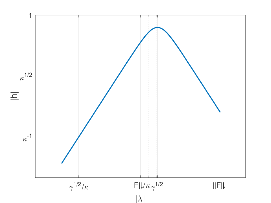
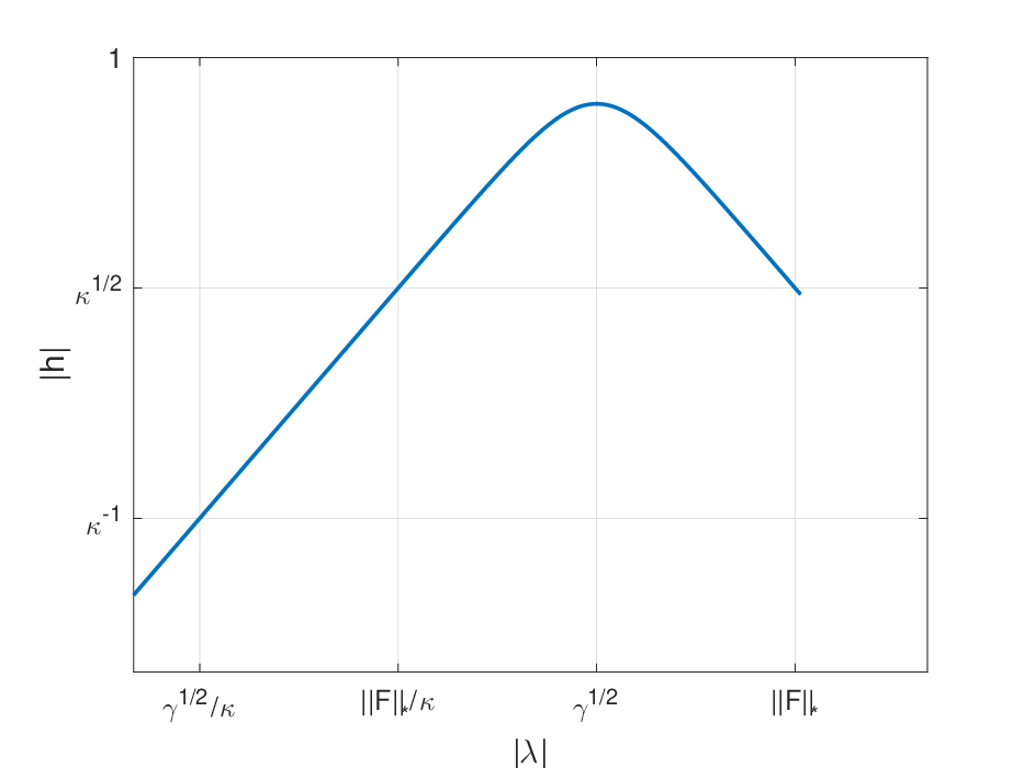
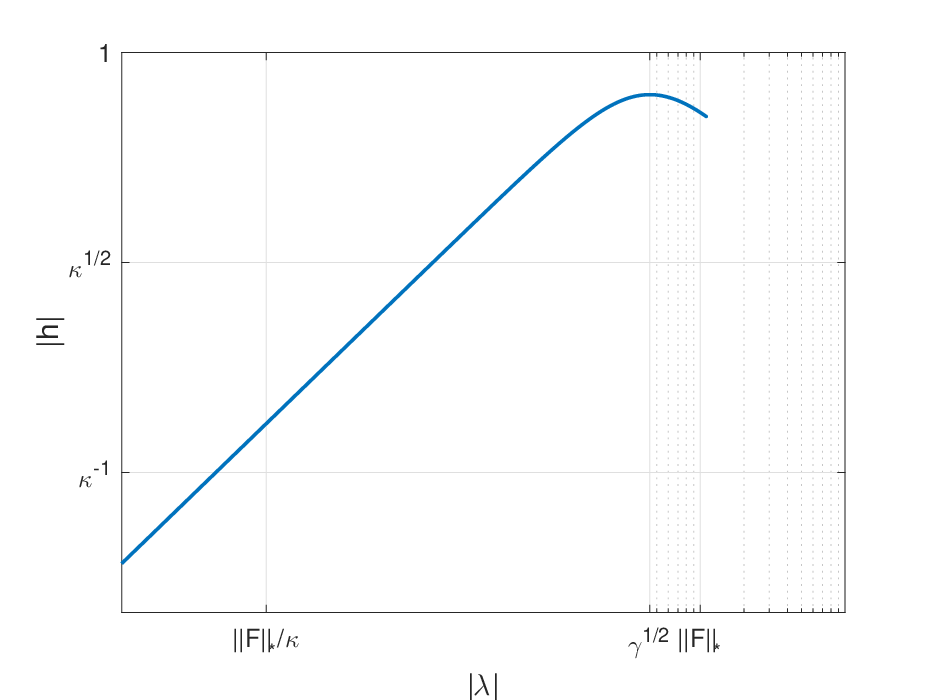
On the other hand, we consider the success probability of the post-selection process. In order to bound the maximal number of iterations, we need to compute the minimum of the rotation function which is related to the hyper-parameter . The image of as a function of is illustrated in Figure 1 33 3 In general, we take . This is reasonable in machine learning area because too small values of lead to a negligible effect of regularization while too large values of result in the loss of useful information of the original problems, i.e., the so-called under-fitting Svergun 1992., from which we see that, for , is given by
Hence, using amplitude amplification Brassard et al. 2002, the number of iterations could be bounded as .
Furthermore, from the experience of machine learning, is usually taken in a logarithmic scale, e.g., 0.01, 0.1, 1, Montavon et al. 1998. Thus we take randomly according to a log-uniform distribution in its domain (Line 1 of Algorithm 1). We estimate the number of iterations as
| (26) |
where obeys a uniform distribution. Combining with (23), the totoal time complexity is . This completes the proof of Theorem 3. ∎
V Further Discussions and Conclusions
In this paper, we proposed a quantum data fitting algorithm for regularized least squares fitting problem with non-sparse matrices, which achieves a runtime of , where the term is due to the random choice of hyper-parameter according to the log-uniform distribution in Algorithm 1. As the hyper-parameter is usually set empirically in machine learning, we let our algorithm generate it automatically. Of course, if one wants to set it manually, he can simply modify our algorithm by moving the first line into the Input.
The technique proposed in this paper could also be applied to HHL algorithm, which would have the same time complexity as WZP Wossnig et al. 2018. It is worth noting that our algorithm’s running time is actually related to the mean of the eigenvalues of , see Eq. (6). If is close to or all the eigenvalues are negative, then the running time is actually relatively small, e.g, maybe logarithmic on the matrix dimension . If , as shown in the case of in Eq. (4), or , then the running time is root quadratic on the matrix dimension, as stated in this paper. However, on the whole, the time complexity of our algorithm is still polynomial in the dimension of the data matrix, because it is derived from the Frobenius norm, or more precisely, from the binary tree data structure Kerenidis and Prakash 2016. Whether there exists a QDF algorithm which runs in logarithmic time on the dimension of non-sparse matrices is still need to be explored.
Acknowledgements.
We thank Prof. Sanjiang Li for helpful discussions and proofreading the manuscript. G. Li acknowledges the financial support from China Scholarship Council (No. 201806070139). This work was partly supported by the Australian Research Council (Grant No: DP180100691) and the Baidu-UTS collaborative project “AI meets Quantum: Quantum algorithms for knowledge representation and learning”.References
- Biamonte et al. (2017) J. Biamonte, P. Wittek, N. Pancotti, P. Rebentrost, N. Wiebe, and S. Lloyd, Nature 549, 195 (2017).
- Wittek (2014) P. Wittek, Quantum machine learning: what quantum computing means to data mining (Academic Press, 2014).
- Harrow et al. (2009) A. W. Harrow, A. Hassidim, and S. Lloyd, Physical review letters 103, 150502 (2009).
- Rebentrost et al. (2014) P. Rebentrost, M. Mohseni, and S. Lloyd, Physical review letters 113, 130503 (2014).
- Kerenidis and Prakash (2016) I. Kerenidis and A. Prakash, arXiv preprint arXiv:1603.08675 (2016).
- Schuld et al. (2016) M. Schuld, I. Sinayskiy, and F. Petruccione, Physical Review A 94, 022342 (2016).
- Wiebe et al. (2014a) N. Wiebe, A. Kapoor, and K. Svore, arXiv preprint arXiv:1401.2142 (2014a).
- Wiebe et al. (2014b) N. Wiebe, A. Kapoor, and K. M. Svore, arXiv preprint arXiv:1412.3489 (2014b).
- Kapoor et al. (2016) A. Kapoor, N. Wiebe, and K. Svore, in Advances in Neural Information Processing Systems (2016) pp. 3999–4007.
- Zhao et al. (2015) Z. Zhao, J. K. Fitzsimons, and J. F. Fitzsimons, arXiv preprint arXiv:1512.03929 (2015).
- Lloyd et al. (2014) S. Lloyd, M. Mohseni, and P. Rebentrost, Nature Physics 10, 631 (2014).
- Low et al. (2014) G. H. Low, T. J. Yoder, and I. L. Chuang, Physical Review A 89, 062315 (2014).
- Rebentrost et al. (2016) P. Rebentrost, M. Schuld, L. Wossnig, F. Petruccione, and S. Lloyd, arXiv preprint arXiv:1612.01789 (2016).
- Ciliberto et al. (2018) C. Ciliberto, M. Herbster, A. D. Ialongo, M. Pontil, A. Rocchetto, S. Severini, and L. Wossnig, Proceedings Of The Royal Society A: Mathematical, Physical and Engineering Sciences 474, 20170551 (2018).
- Wiebe et al. (2012) N. Wiebe, D. Braun, and S. Lloyd, Physical review letters 109, 050505 (2012).
- Childs (2010) A. M. Childs, Communications in Mathematical Physics 294, 581 (2010).
- Berry and Childs (2009) D. W. Berry and A. M. Childs, arXiv preprint arXiv:0910.4157 (2009).
- Liu and Zhang (2015) Y. Liu and S. Zhang, in International Workshop on Frontiers in Algorithmics (Springer, 2015) pp. 204–216.
- Hawkins (2004) D. M. Hawkins, Journal of chemical information and computer sciences 44, 1 (2004).
- Hoerl and Kennard (1970) A. E. Hoerl and R. W. Kennard, Technometrics 12, 55 (1970).
- Wossnig et al. (2018) L. Wossnig, Z. Zhao, and A. Prakash, Physical review letters 120, 050502 (2018).
- Meng et al. (2018) F.-X. Meng, X.-T. Yu, R.-Q. Xiang, and Z.-C. Zhang, IEEE Access (2018).
- Yu et al. (2017) C.-H. Yu, F. Gao, and Q.-Y. Wen, arXiv preprint arXiv:1707.09524 (2017).
- Kitaev (1995) A. Y. Kitaev, arXiv preprint quant-ph/9511026 (1995).
- Svergun (1992) D. Svergun, Journal of applied crystallography 25, 495 (1992).
- Brassard et al. (2002) G. Brassard, P. Hoyer, M. Mosca, and A. Tapp, Contemporary Mathematics 305, 53 (2002).
- Montavon et al. (1998) G. Montavon, G. B. Orr, and K.-R. Müller, (1998).