\RS@ifundefined

subsecref name = \RSsectxt \RS@ifundefinedthmref name = theorem \RS@ifundefinedlemref name = lemma

Graphs with large girth and free groups

Ofir David Email address: eofirdavid@gmail.com

Abstract.

We use Margulis’ construction together with lattice counting arguments to build Cayley graphs on $\mathrm{SL}_{2}\left(\mathbb{F}_{p}\right),\;p\to\infty$ which are $d$ -regular graphs with girth $\geq\frac{2}{3}\frac{\ln\left(n\right)}{\ln\left(d-1\right)+\ln\left(C\right)}$ for some absolute constant $C$ .

1. Introduction

Starting with an empty graph on $n$ vertices, we can add $n-1$ edges without creating any cycle, thus getting a tree, and every edge after that must create a new cycle. However, if we choose the placements of these new edges carefully, we can make sure that at least locally our graph still looks like a tree, or equivalently we do not form small cycles. We call the length of the shortest simple cycle the girth of the graph and we denote it by $\mathfrak{g}$ .

Clearly, if we add too many edges than we must have small cycles. To be more specific, suppose that we have a $d$ -regular graph $\Gamma$ on $n$ -vertices with an even girth $\mathfrak{g}=2m$ (though a similar result holds for odd girth). In this case, any ball of radius $m-1$ in the graph is a tree, and since our graph is $d$ -regular, this tree has $1+d\frac{\left(d-1\right)^{m-1}-1}{d-2}\geq\left(d-1\right)^{m-1}$ vertices. It follows that $n\geq\left(d-1\right)^{m-1},$ and by taking the logarithm

1+2\frac{\ln\left(n\right)}{\ln\left(d-1\right)}\geq\mathfrak{g}.

Thus, we see that if we fix the number of vertices $n$ , then we can’t have that both the girth $\mathfrak{g}$ is large and the number of edges, which is controlled by $d$ , is too large.

On the other hand, we can ask what is the largest girth possible for a $d$ -regular graph on $n$ vertices, and with this upper bound in mind, define $C\left(n,d\right)$ to be the largest number such that there exists a $d$ -regular graph on $n$ vertices with

\mathfrak{g}\geq C\left(n,d\right)\frac{\ln\left(n\right)}{\ln\left(d-1\right)}.

The argument above shows that $C\left(n,d\right)\leq 2$ (up to the $+1$ ). One of the first lower bounds for $C\left(n,d\right)$ was given by Erdös and Saks in [1], where they used a counting method to show the existence of graphs with $\mathfrak{g}\geq\frac{\ln\left(n\right)}{\ln\left(d-1\right)}\left(1-o\left(n\right)\right)$ . However, probably the first explicit construction is by Margulis in [9] where he showed that Cayley graphs of $\mathrm{SL}_{2}\left(\mathbb{F}_{p}\right)$ with the generators

S=\left\{\left(\begin{array}[]{cc}1&\pm 2\\ 0&1\end{array}\right),\left(\begin{array}[]{cc}1&0\\ \pm 2&1\end{array}\right)\right\}

form a family of $4$ -regular graphs with $\mathfrak{g}\geq\frac{2\cdot\ln\left(3\right)}{3\ln\left(1+\sqrt{2}\right)}\frac{\ln\left(n\right)}{\ln\left(4-1\right)}$ so that $C\left(n,4\right)\geq\frac{2\cdot\ln\left(3\right)}{3\ln\left(1+\sqrt{2}\right)}\sim 0.831$ , and for general $d$ he shows that $C\left(n,d\right)\geq\frac{4}{9}$ . One of the interesting components of this proof is that $S$ can be viewed as a subset of $\mathrm{SL}_{2}\left(\mathbb{Z}\right)$ , and there it generates a (finite index) free subgroup, so that its Cayley graph is the $4$ -regular tree (and similar arguments were used for general $d$ ). Thus, the projections of groups $\left\langle S\right\rangle_{\mathrm{SL}_{2}\left(\mathbb{Z}\right)}\to\left\langle S\right\rangle_{\mathrm{SL}_{2}\left(\mathbb{F}_{p}\right)}=\mathrm{SL}_{2}\left(\mathbb{F}_{p}\right)$ induce covering maps from the $4$ -regular tree to the finite graphs in Margulis’ construction. These graphs should be thought of as being better and better approximations of the universal covering tree, and what Margulis is showing is that this approximation is in a sense “uniform” (locally, the graphs look like trees) and “fast” (the girth is growing logarithmically in $n$ ). Margulis result was later improved using similar ideas by Imrich in [5] where he showed that $C\left(n,d\right)\geq 0.48$ .

One of the main benefits of working with Cayley graphs is that they have many symmetries, and in particular they are vertex transitive. It follows that in order to show that there are no small cycles, we “only” need to show that in a small neighborhood of a single vertex, so in a sense we get the “uniformity” condition above automatically. Furthermore, once we work with Cayley graphs, we have all the tools from group theory in our disposal, which usually make things easier and more interesting.

A second important construction leading to graphs with high girth are the LPS graphs which were constructed by Lubotzky, Philips and Sarnak (see [8]). These graphs are actually Ramanujan graphs which are in a sense the best possible expander graphs, and one of the properties of these graphs is that they have high girth. As in Margulis’ construction, the LPS graphs also arise from an algebraic construction, this time from quaternion algebras, which in a sense are very close to be matrix algebras, and here too there is a free group which hides in the background. There are two types of LPS graphs, on $\mathrm{PSL}_{2}\left(\mathbb{F}_{p}\right)$ and $\mathrm{PGL}_{2}\left(\mathbb{F}_{p}\right)$ respectively where the first satisfies $\mathfrak{g}\geq\frac{2}{3}\frac{\ln\left(n\right)}{\ln\left(d-1\right)}$ and the other $\mathfrak{g}\geq\frac{4}{3}\frac{\ln\left(n\right)}{\ln\left(d-1\right)}$ . In these graphs also one of the main component is to lift the graphs, but instead of lifting to $\mathrm{PGL}_{2}\left(\mathbb{Z}\right)$ , we lift them to the $p$ -adic group $\mathrm{PGL}_{2}\left(\mathbb{Z}_{p}\right)$ . When we run over the different primes $p$ (which can be put together inside the adeles), we produce the different graphs. Thus, once again we have a sort of a universal object, such that our family of graphs is just increasing quotients of this object.

Other than these two construction, there are many more constructions, see for example [6, 7], though the LPS graphs still have the best result for large girth. In this paper, we revisit Margulis’ first construction and improve it to get a family with $\mathfrak{g}\geq\frac{2}{3}\frac{\ln\left(n\right)}{\ln\left(d-1\right)}$ . While this doesn’t improve upon the currently known results, it does however uses a combination of ideas from combinatorics and group theory which we find very interesting. Moreover, it also leads to questions regarding lattice counting problems which seem natural and might suggest generalization of this construction.

Theorem 1.1.

There exists an absolute constant $\tilde{C}$ and $W_{R}\subseteq\mathrm{SL}_{2}\left(\mathbb{Z}\right)$ such that $W_{R}$ is a symmetric basis for a free group, and the connected components $\Gamma_{p}$ of the identity of the Cayley graph $Cay\left(\mathrm{SL}_{2}\left(\mathbb{F}_{p}\right),W_{R}\right)$ satisfy

\left\lceil\frac{\mathfrak{g}}{2}\right\rceil\geq\frac{1}{3}\frac{\ln\left(n_{p}\right)}{\ln\left|W_{R}\right|+\ln\left(\tilde{C}\right)},\quad n_{p}=\text{number of vertices in }\text{$\Gamma_{p}$}.

1.1. Acknowledgment

I would like to thank Ami Paz for first introducing me to this problem of finding graphs with large girth.

The research leading to these results has received funding from the European Research Council under the European Union Seventh Framework Programme (FP/2007-2013) / ERC Grant Agreement n. 335989.

2. Constructing the graphs

As mentioned before, our construction uses Cayley graphs of $\mathrm{SL}_{2}\left(\mathbb{F}_{p}\right)$ . The basic argument for the lower bound on the girth is the same as in Margulis’ paper, while the difference will be in the choice of generators which is related to lattice counting problems. With this in mind, in section 2.1 we start by recalling Margulis’ proof, then in section 2.2 we begin to study how to construct free subgroups in $\mathrm{SL}_{2}\left(\mathbb{Z}\right)$ by considering them as fundamental groups of graphs. Finally, in 2.3 we use these ideas to show how to construct sets of generators which produce Cayley graphs with high girth.

2.1. Cayley graphs and Margulis’ proof

We begin with the construction of Cayley graphs which will be our examples of graphs with high girth.

Definition 2.1.

Let $G$ be a group and $S\subseteq G$ a set. The Cayley graph $Cay\left(G,S\right)$ is the directed graph with $G$ as the set of vertices and the edges $E=\left\{g\to gs\;\mid\;\forall g\in G,\;s\in S\right\}$ . We define a labeling on the edges $L:E\to S$ by $L\left(g\to gs\right)=s$ .

Given an element $g\in G$ and a tuple $\bar{s}=\left(s_{1},...,s_{k}\right)\in S^{k}$ for some $k$ , we define the path $P_{g,\bar{s}}$ to be

P_{g,\bar{s}}=g\to gs_{1}\to gs_{1}s_{2}\to\cdots\to gs_{1}\cdots s_{k}.

The Cayley graphs are highly symmetric, and many of their combinatorial properties can be formulated using the group $G$ .

Lemma 2.2.

Let $G$ be a group and $S\subseteq G$ .

(1)

The underlying undirected graph of $Cay\left(G,S\right)$ is connected if and only if $S$ generates $G$ .
(2)

The standard left action of $G$ on itself induces a left action of $G$ on $Cay(G,S)$ . In particular $Cay\left(G,S\right)$ is vertex transitive.
(3)

A path $P_{g,\bar{s}},\;g\in G,\;\bar{s}\in S^{d}$ is nonbacktracking if and only if $s_{i}s_{i+1}\neq e$ for each $i$ , and it is a cycle if and only if $s_{1}s_{2}\cdots s_{d}=e$ . In particular, the distance in the graph between $g$ and $gh$ is the word length of $h$ over the elements in $S$ (which is infinite if $h\notin\left\langle S\right\rangle$ ).

Proof.

These are all pretty easy, and we leave it as an exercise. ∎

Example 2.3.

For $G=D_{6}$ the dihedral group with 6 elements and $S=\left\{r,s\right\}$ where $r$ is the rotation and $s$ the reflection, we get the following Cayley graph

If $S=S^{-1}$ is symmetric, then whenever $g\mapsto gs$ is an edge, we also have the edge $gs\mapsto g=\left(gs\right)s^{-1}$ . In this case we will also think of $Cay\left(G,S\right)$ as an undirected graph (after identifying these pair of edges), so we may talk about the girth $\mathfrak{g}\left(Cay\left(G,S\right)\right)$ . As with the lemma above, this too can be formulated in the language of $G$ and $S$ .

Lemma 2.4.

Let $G$ be a finite group and $S=S^{-1}\subseteq G$ . Then the girth $\mathfrak{g}\left(Cay\left(G,S\right)\right)$ is the smallest $d$ such that $\exists s_{i}\in S,\;i=1,...,d$ with $s_{i}s_{i+1}\neq e$ and $\prod_{1}^{d}s_{i}=e$ .

Things begin to be interesting when we have a homomorphism $\varphi:G\to H$ and for simplicity assume that $\varphi\mid_{S}$ is injective, so we can identity $S$ with $\varphi\left(S\right)$ . Such a homomorphism will induce a graph homomorphism $\tilde{\varphi}:Cay\left(G,S\right)\to Cay\left(H,\varphi\left(S\right)\right)$ , so if $S$ is symmetric we immediately get that

\mathfrak{g}\left(Cay\left(G,S\right)\right)\geq\mathfrak{g}\left(Cay\left(H,\varphi\left(S\right)\right)\right).

Margulis’ idea was to fix $G=\mathrm{SL}_{2}\left(\mathbb{Z}\right)$ , and to study the standard congruence morphisms $\pi_{p}:\mathrm{SL}_{2}\left(\mathbb{Z}\right)\to\mathrm{SL}_{2}\left(\mathbb{F}_{p}\right)$ (and note that $\pi_{p}\mid_{S}$ is injective for almost every $p$ ). If we ever hope to get such a family with some lower bound $\mathfrak{g}\geq c\frac{\ln\left(n\right)}{\ln\left(d-1\right)}$ , then by the argument above the Cayley graph on $\mathrm{SL}_{2}\left(\mathbb{Z}\right)$ must be a tree. The connected components of a Cayley graph $Cay\left(G,S\right)$ are trees if and only if we cannot write $\prod_{1}^{d}s_{i}=e$ (a cycle) without $s_{i}s_{i+1}=e$ for some $i$ (backtracking), so that $S$ is a basis for a free group. Hence, a good place to look for graphs with high girth, is with projections of a Cayley graph of a free subgroup of $\mathrm{SL}_{2}\left(\mathbb{Z}\right)$ .

Once the problem is in $Cay\left(\mathrm{SL}_{2}\left(\mathbb{Z}\right),S\right)$ , Margulis used the fact that we can use norms on $\mathrm{SL}_{2}\left(\mathbb{Z}\right)$ . So before we give the main idea of his proof, we need one definition for norms.

Definition 2.5.

Given a norm $\left\|\cdot\right\|$ on $M_{2}\left(\mathbb{R}\right)$ , let $\eta\left(\left\|\cdot\right\|\right)=\sup_{g,h\in\mathrm{SL}_{2}\left(\mathbb{Z}\right)}\frac{\left\|g\right\|\left\|h\right\|}{\left\|gh\right\|}$ .

Example 2.6.

(1)

If the norm is multiplicative, for example the operator norm or the $l_{2}$ -norm, then $m\left(\left\|\cdot\right\|\right)=1$ .
(2)

For the max norm, it is easy to check that $\eta\left(\left\|\cdot\right\|_{\infty}\right)=2$ .

Lemma 2.7.

Let $F\leq\mathrm{SL}_{2}\left(\mathbb{Z}\right)$ be a free group over a symmetric set $S=\left\{s_{1}^{\pm 1},...,s_{d}^{\pm 1}\right\}$ , and let $p$ be a prime such that $\pi_{p}\mid_{S}$ is injective. Let $\left\|\cdot\right\|$ be any norm on $M_{2}\left(\mathbb{R}\right)$ bigger than $\left\|\cdot\right\|_{\infty}$ , and set $\eta=\eta\left(\left\|\cdot\right\|\right)$ and $M={\displaystyle\max_{s\in S}}\left\|s\right\|$ . Then for $\mathfrak{g}=girth\left(Cay\left(\mathrm{SL}_{2}\left(p\right),S\right)\right)$ we get that $\left(\eta M\right)^{\left\lceil\mathfrak{g}/2\right\rceil}\geq\frac{\eta p}{2}$ .

Proof.

Suppose that $\prod_{1}^{k}t_{i}\equiv_{p}I$ with $t_{i}\in S$ and $t_{i}t_{i+1}\not\equiv_{p}I$ , and in particular $t_{i}t_{i+1}\neq I$ . Since $F$ is free over $S$ this implies that $\prod_{1}^{k}t_{i}\neq I$ . Combinatorially speaking, a nonbacktracking cycle in $Cay\left(\mathrm{SL}_{2}\left(\mathbb{F}_{p}\right),S\right)$ always lifts to a nonbacktracking path in $Cay\left(\mathrm{SL}_{2}\left(\mathbb{Z}\right),S\right)$ which is not a cycle.

Using the fact that $\mathrm{SL}_{2}\left(\mathbb{Z}\right)$ sits inside $M_{2}\left(\mathbb{Z}\right)$ , we get that that $\prod_{1}^{\left\lfloor k/2\right\rfloor}t_{i}-\prod_{k}^{\left\lfloor k/2\right\rfloor+1}t_{i}^{-1}\neq 0$ over $\mathbb{Z}$ , while it is 0 mod $p$ , which implies that

2\cdot\max\left\{\left\|\prod_{1}^{\left\lfloor k/2\right\rfloor}t_{i}\right\|,\left\|\prod_{k}^{\left\lfloor k/2\right\rfloor+1}t_{i}^{-1}\right\|\right\}\geq\left\|\prod_{1}^{\left\lfloor k/2\right\rfloor}t_{i}-\prod_{k}^{\left\lfloor k/2\right\rfloor+1}t_{i}^{-1}\right\|\geq\left\|\prod_{1}^{\left\lfloor k/2\right\rfloor}t_{i}-\prod_{k}^{\left\lfloor k/2\right\rfloor+1}t_{i}^{-1}\right\|_{\infty}\geq p.

Since $\left\|gh\right\|\leq\eta\left\|g\right\|\left\|h\right\|$ for any $g,h\in\mathrm{SL}_{2}\left(\mathbb{R}\right)$ , it follows that $\frac{\left(\eta M\right)^{\left\lceil k/2\right\rceil}}{\eta}\geq\frac{p}{2}$ which completes the proof. ∎

If the elements of $S$ are distinct mod $p$ , then $Cay\left(\mathrm{SL}_{2}\left(\mathbb{F}_{p}\right),S\right)$ is $\left|S\right|$ -regular. Given the lemma above, we want to find a set $S=S^{-1}$ which is a basis of a free subgroup of $\mathrm{SL}_{2}\left(\mathbb{Z}\right)$ where $M={\displaystyle\max_{s\in S}}\left\|s\right\|_{\infty}$ is as small as possible, thus producing a graph with a high girth.

In Margulis’ construction in [9], he uses

S=\left\{\left(\begin{array}[]{cc}1&\pm 2\\ 0&1\end{array}\right),\left(\begin{array}[]{cc}1&0\\ \pm 2&1\end{array}\right)\right\}

and the operator norm, so that $\eta=1$ and $M=1+\sqrt{2}$ . Additionally, we have that $n=\left|\mathrm{SL}_{2}\left(\mathbb{F}_{p}\right)\right|=p\left(p^{2}-1\right)$ , $d=4$ and $\mathrm{SL}_{2}\left(\mathbb{F}_{p}\right)$ is generated by $S$ . Therefore by the lemma above we get that

\left\lceil\mathfrak{g}/2\right\rceil\geq\frac{\ln\left(\frac{p}{2}\right)}{\ln\left(1+\sqrt{2}\right)}=\frac{1}{3}\frac{\ln\left(p^{3}\right)-\ln\left(8\right)}{\ln\left(1+\sqrt{2}\right)}\geq\frac{\ln\left(3\right)}{3\ln\left(1+\sqrt{2}\right)}\frac{\ln\left(n\right)-\ln\left(8\right)}{\ln\left(4-1\right)}.

Thus, this gives a construction with $\mathfrak{g}\geq 0.831...\cdot\frac{\ln\left(n\right)}{\ln\left(d-1\right)}$ .

Remark 2.8.

In general, fixing the norm, if $d$ is big, then $M$ is going to be big, so in the result of the 2.7, after taking the logarithm, the constant $\eta$ will be negligible. In particular this will be true if we let $d$ grow to infinity as well. In this case we can simply think of the result (asymptotically) as

\mathfrak{g}\geq\frac{2}{3}\frac{\ln\left(n\right)}{\ln\left(M\right)}.

In the rest of these notes we will only use the infinity norm, though for small $d$ , one might try to optimize the choice of the norm to get better results.

2.2. Free groups and graph covers

Now that we have the basic idea of the proof and its relation to free groups, we continue to construct free subgroups as fundamental groups of graph covers.

Consider the following example of a labeled graph (defined below).

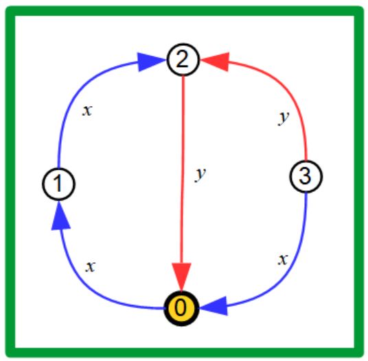
Refer to caption — Figure 2.1. A labeled graph.

It has two “main” cycles corresponding to $x^{2}y$ on the left and $x^{-1}y^{2}$ on the right, and every other cycle can be constructed using these two cycles (up to homotopy, i.e. modulo backtracking). Furthermore, the labeling allows us to think of these cycles as elements in $F_{2}=\left\langle x,y\right\rangle$ , so that the fundamental group of the graph could be considered as the subgroup generated by $x^{2}y$ and $x^{-1}y^{2}$ . With this example in mind, we now give the proper definitions to make this argument more precise.

One of the most basic results in algebraic topology is that the fundamental group of a graph is always a free group. Let us recall some of the details.

Definition 2.9 (Cycle basis).

Let $\Gamma$ be a connected undirected graph with a special vertex $v\in V\left(\Gamma\right)$ , and let $T\subseteq E\left(\Gamma\right)$ be a spanning tree. For each edge $e:u\to w$ let $C_{e}$ be the simple cycle going from $v$ to $u$ on the unique path in the tree $T$ , then from $u$ to $w$ via $e$ and finally from $w$ to $v$ via $T$ . We denote by $C\left(T\right)=\left\{e\notin T\;\mid\;C_{e}\right\}$ this collection of cycles.

It is not hard to show that any cycle in a connected graph can be written as a concatenation of cycles in $C\left(T\right)$ and their inverses as elements in the fundamental group $\pi_{1}\left(\Gamma\right)$ (namely, we are allowed to remove backtracking). More over, it has a unique such presentation which leads to the following:

Corollary 2.10.

Let $\Gamma$ be a graph and $T$ a spanning tree. Then $C\left(T\right)$ is a basis for $\pi_{1}\left(\Gamma\right)$ which is a free group on $\left|E\left(\Gamma\right)\right|-\left|V\left(\Gamma\right)\right|+1$ elements.

Example 2.11.

In 2.1 the edge touching the 0 vertex form a spanning tree, and then $C_{\left(1,2\right)}=0\overset{x}{\to}1\overset{x}{\to}2\overset{y}{\to}0$ and $C_{\left(3,2\right)}=0\overset{x}{\leftarrow}3\overset{y}{\to}2\overset{y}{\to}0$ , so that eventually we will think of the fundamental group as generated by $x^{2}y$ and $x^{-1}y^{2}$ per our intuition from the start of this section.

In particular, the corollary above implies that the fundamental group of the bouquet graph with a single vertex and $n$ self loops is the free group $F_{n}$ . We can label the edges by the corresponding basis elements $x_{1},...,x_{n}$ in $F_{n}=\left\langle x_{1},...x_{n}\right\rangle$ . Since it is important in which direction we travel across the edge, we will think of each edge as two directed edges labeled by $x_{i}$ and $x_{i}^{-1}$ depending on the image in the fundamental group. For simplicity, we will keep only the edges with the $x_{i}$ labeling, understanding that we can also travel in the opposite direction via an $x_{i}^{-1}$ labeled edge.

It is well known that a fundamental group of a covering space correspond to a subgroup of the original space. Using the generalization of the labeling above we can produce covering using the combinatorics of labeled graphs.

For the rest of this section we fix a basis $x_{1},...,x_{n}$ of the free group $F_{n}$ .

Definition 2.12.

A labeled graph $\left(\Gamma,v\right)$ is a directed graph $\Gamma$ with a special vertex $v$ , where the edges are labeled by $x_{1},...,x_{n}$ (see 2.2). A labeled graph morphism $\left(\Gamma_{1},v_{1}\right)\to\left(\Gamma_{2},v_{2}\right)$ between labeled graphs is a morphism of graphs $\Gamma_{1}\to\Gamma_{2}$ which sends $v_{1}$ to $v_{2}$ and preserves the labels on the edges.

We denote by $\Gamma_{F_{n}}$ the bouquet graph with the $x_{1},...,x_{n}$ labeling. Note that another way to define a labeling on a graph $\Gamma$ is a morphism of directed graphs $\varphi:\Gamma\to\Gamma_{F_{n}}$ where the labeling of an edge $e\in E\left(\Gamma\right)$ is defined to be the labeling of $\varphi\left(e\right)$ . In this way a labeled graph morphism is just a map which defines a commuting diagram

This labeling map $\varphi:\Gamma\to\Gamma_{F_{n}}$ induces a homomorphism $\hat{\varphi}:\pi_{1}\left(\Gamma,v\right)\to\pi_{1}\left(\Gamma_{F_{n}}\right)=F_{n}$ . Since every path in $\Gamma$ is sent to a cycle in $\Gamma_{F_{n}}$ , we can extend this map to general paths in $\Gamma$ .

Definition 2.13.

Let $\left(\Gamma,v\right)$ be a graph with a labeling $\varphi:\Gamma\to\Gamma_{F_{n}}$ . Given a path $P$ in $\Gamma$ starting at $v$ , define the labeling $L\left(P\right)$ of the path to be the (cycle) element $\varphi\left(P\right)$ in the fundamental group $\pi_{1}\left(F_{n}\right)$ . In other words, this is just the element in $F_{n}$ created by the labels on the path.

In general, for a labeled graph $\varphi:\Gamma\to\Gamma_{F_{n}}$ the function $\hat{\varphi}$ is not injective. However, in the Stallings graphs case, defined below, it is.

Definition 2.14.

A Stallings graph is a labeled graph $\varphi:\left(\Gamma,v\right)\to\Gamma_{F_{n}}$ where $\varphi$ is locally injective, namely for every vertex $u\in V\left(\Gamma\right)$ and every $i=1,...,n$ there is at most one outgoing edge from $u$ and at most one ingoing edge into $u$ labeled by $x_{i}$ . We call the graph a covering graph if $\varphi$ is a local homeomorphism, or equivalently every vertex has exactly one ingoing and one outgoing labeled by $x_{i}$ for every $i$ .

Remark 2.15.

Given a covering graph, we can remove every edge and vertex which are not part of a simple cycle so as to not change the fundamental group. The resulting graph will be a Stallings graph, and conversely, every Stallings graph can be extended to a covering graph of $\Gamma_{F_{n}}$ without changing the fundamental domain.

In the Stallings graph case, it is an exercise to show that $\hat{\varphi}$ is injective, and we may consider $\pi_{1}\left(\Gamma,v\right)$ as a subgroup of $F_{n}$ . Moreover, we can use 2.9 to find a basis for $\pi_{1}\left(\Gamma,v\right)$ as a subgroup of $F_{n}$ .

Example 2.16.

In 2.2 below, in the left most graph, the path

P:=v_{0}\overset{x}{\longrightarrow}v_{1}\overset{y}{\longrightarrow}v_{2}\overset{y}{\longrightarrow}v_{0}\overset{y}{\longleftarrow}v_{0}

is labeled by $L\left(P\right)=xyyy^{-1}=xy$ . Similarly, in the second graph from the right the path

P:=v_{0}\overset{x}{\longrightarrow}v_{1}\overset{y}{\longrightarrow}v_{2}\overset{x}{\longleftarrow}v_{3}\overset{y}{\longleftarrow}v_{0}

is labeled by $\pi_{1}\left(P\right)=xyx^{-1}y^{-1}=\left[x,y\right]$ .

The images $\hat{\varphi}\left(\Gamma,v\right)$ for the graphs in this figure from left to right are $\left\langle xy,xy^{2},y\right\rangle=\left\langle x,y\right\rangle,\;\left\langle y,xyx^{-1}\right\rangle$ , $\left\langle xyx^{-1}y^{-1}\right\rangle$ and $\left\langle x,y\right\rangle$ . Note that the fundamental group of the left most graph is free of rank $3$ (there are 3 loops in the graph) while the image $\hat{\varphi}\left(\Gamma,v\right)=\left\langle x,y\right\rangle$ is generated by only two element, which in particular indicates that it is not a Stallings graph.

2.3. Finding good generators

Our final task is to construct graph covering, and to choose generators which are small (so that $M$ in 2.7 will be small). In this section we will use the infinity norm, and just write $\left\|\cdot\right\|$ instead of $\left\|\cdot\right\|_{\infty}$ . We will keep $S$ as the set

S=\left\{A,B\right\},\quad A=\left(\begin{array}[]{cc}1&2\\ 0&1\end{array}\right),\;B=\left(\begin{array}[]{cc}1&0\\ 2&1\end{array}\right)

and we will look for free subgroups in $\left\langle S\right\rangle$ . As such, all of our graphs will be $S$ labeled (with our usual convention for $A^{-1},B^{-1}$ labeled edges).

All of the elements in $S\cup S^{-1}$ are very “similar” and in particular have the same norm. To make this even more precise, we consider the following.

Definition 2.17.

For $g\in\mathrm{SL}_{2}\left(\mathbb{Z}\right)$ define $\sigma\left(g\right)=\left(g^{-1}\right)^{T}$ and $\tau\left(g\right)=\left(\begin{array}[]{cc}0&1\\ 1&0\end{array}\right)g\left(\begin{array}[]{cc}0&1\\ 1&0\end{array}\right)$ .

Lemma 2.18.

The elements $\sigma$ and $\tau$ are commuting automorphisms of $\mathrm{SL}_{2}\left(\mathbb{R}\right)$ and each has order 2, so that $\left\langle\sigma,\tau\right\rangle=\left\{e,\sigma,\tau,\sigma\tau\right\}$ . Moreover, $S\cup S^{-1}$ is a single orbit of $\left\langle\sigma,\tau\right\rangle$ and for any $g\in\mathrm{SL}_{2}\left(\mathbb{R}\right)$ we have that $\left\|g\right\|=\left\|\tau\left(g\right)\right\|=\left\|\sigma\left(g\right)\right\|$ .

Proof.

Left as an exercise. ∎

We now use this symmetry to construct good free subgroups of $\left\langle S\right\rangle$ . The main idea will be to start with the 4-regular tree $Cay\left(\mathrm{SL}_{2}\left(\mathbb{Z}\right),S\right)$ , and for a fixed $R$ to look on the subgraph of the matrices $g$ with $\left\|g\right\|\leq R$ . We will then complete this graph to create a covering graph of $\Gamma_{F_{2}}$ . The bound on $\left\|g\right\|$ will imply that the max norm of our generators will be small, and then we are left with the problem of counting how many elements satisfy $\left\|g\right\|\leq R$ .

Lemma 2.19.

There exists an absolute constant $C$ such that for any $R>0$ there exists a free subgroup $F=F_{R}\leq\left\langle S\right\rangle$ over a symmetric set $W=W_{R}$ satisfying:

(1)

$W=\sigma\left(W\right)=\tau\left(W\right)$ .
(2)

${\displaystyle\max_{w\in W}}\left\|w\right\|\leq 18R^{2}$ .
(3)

$\left|W\right|\geq CR^{2}$ .
(4)

The elements of $W$ are distinct mod $p$ for $p>36\cdot R^{2}$ .

Proof.

Let $\Gamma^{\prime\prime}$ be the connected component of the identity in $Cay\left(\mathrm{SL}_{2}\left(\mathbb{Z}\right),S\right)$ which is a 4-regular tree with the natural $S$ labeling. Given $R>0$ , let $\Omega_{R}=\left\{g\in\left\langle S\right\rangle:\left\|g\right\|\leq R\right\}$ and set $\Gamma^{\prime}=\left(V^{\prime},E^{\prime}\right)$ to be the smallest connected subgraph of $\Gamma^{\prime\prime}$ which contains $\Omega_{R}$ (actually, it can be shown that $V^{\prime}=\Omega_{R}$ ). Since $\sigma$ and $\tau$ preserve both $S^{\pm 1}$ and the norm, it also acts on $\Gamma^{\prime}$ . The graph $\Gamma^{\prime}$ is an $S$ labeled tree and we want to complete it to be a covering of $\Gamma_{F_{2}}$ .

Let $g\in V^{\prime}$ and $s\in S\cup S^{-1}$ such that $\left(g,gs\right)\notin E^{\prime}$ , or equivalently $gs\notin V^{\prime}$ . Applying $\sigma$ we obtain that $\sigma\left(g\right)\in V^{\prime}$ while $\left(\sigma\left(g\right),\sigma\left(g\right)\sigma\left(s\right)\right)\notin E^{\prime}$ . For each such pair $\left\{\left(g,gs\right),\left(\sigma\left(g\right),\sigma\left(gs\right)\right)\right\}$ we add to $\Gamma^{\prime}$ the vertex $v_{g,s}$ , and two labeled edges $g\overset{s}{\to}v_{g,s}\overset{s^{T}}{\to}g^{-T}$ . In addition, define $C_{g,s}$ to be the cycle defined by $e\rightsquigarrow g\overset{s}{\to}v_{g,s}\overset{s^{T}}{\to}\sigma\left(g\right)\rightsquigarrow e$ where the $\rightsquigarrow$ arrow is the unique path in the tree $\Gamma^{\prime}$ . We let $\Gamma=\left(V,E\right)$ be the new graph after doing this construction for each such pair, which construction is a Stallings graph. Letting $W_{+}$ be the collection of cycles which we just constructed, it is easily seen to be a cycle basis for $\Gamma$ , and therefore they generate $\pi_{1}\left(\Gamma\right)$ , and we need to show that $W_{R}:=W_{+}\cup W_{+}^{-1}$ satisfy the conditions in this lemma.

Note first that since by construction $\Gamma$ is a Stallings graph, we can identify these cycles with elements in $\left\langle S\right\rangle$ via their labels, namely we identify $C_{g,s}\sim L\left(C_{g,s}\right)=\left(gs\right)\left(gs\right)^{T}$ . Since $\sigma$ and $\tau$ preserve the norm, by the definition of these cycles we get that $W_{R}$ is invariant under $\sigma$ and $\tau$ which is condition (1).

Secondly, by definition for each cycle $C_{g,s}$ we have that $\left\|gs\right\|\leq 3\left\|g\right\|\leq 3R$ , so that

\left\|\left(gs\right)\left(gs\right)^{T}\right\|\leq 2\left\|gs\right\|^{2}\leq 18R^{2},

which is part (2).

Next we want to find the size of $W_{R}$ . For that, note first that each edge in $E$ touches a vertex from $V^{\prime}$ and each such vertex in $V^{\prime}$ has exactly two outgoing edges (labeled by $A$ and $B$ respectively), hence $\left|E\right|=2\left|V^{\prime}\right|$ . Recall that $\Gamma^{\prime}$ is a tree so it has $\left|E^{\prime}\right|=\left|V^{\prime}\right|-1$ edges, and any cycle $C_{g,s}$ uses exactly 2 edges in $E\backslash E^{\prime}$ . Finally, two distinct cycles use different edges, so the number of these cycles is

\frac{\left|E\right|-\left|E^{\prime}\right|}{2}=\frac{2\left|V^{\prime}\right|-\left(\left|V^{\prime}\right|-1\right)}{2}=\frac{\left|V^{\prime}\right|+1}{2},

so we are left to count the number of vertices in $V^{\prime}$ which is exactly the number of matrices in $\left\langle S\right\rangle$ with norm $\leq R$ .

It is well known that $\mathrm{SL}_{2}\left(\mathbb{Z}\right)$ is a lattice in $\mathrm{SL}_{2}\left(\mathbb{R}\right)$ , namely it is discrete and $\nicefrac{{\mathrm{SL}_{2}\left(\mathbb{R}\right)}}{{\mathrm{SL}_{2}\left(\mathbb{Z}\right)}}$ has finite volume. Moreover, since $\left[\mathrm{SL}_{2}\left(\mathbb{Z}\right):\left\langle S\right\rangle\right]=12<\infty$ , the group $\left\langle S\right\rangle$ is also a lattice in $\mathrm{SL}_{2}\left(\mathbb{R}\right)$ . By [3] there is some absolute constant $C$ such that $\left|V^{\prime}\right|\geq CR^{2}$ , which finishes part (3). For completeness, we added an elementary proof for this lower bound in the A.

Finally, assume that $w_{1},w_{2}\in W$ such that $w_{1}\equiv_{p}w_{2}$ where $2\cdot 18R^{2}<p$ . Since
$\left\|w_{1}-w_{2}\right\|_{\infty}\leq 2\cdot 18R^{2}<p$ , we must have that $w_{1}=w_{2}$ which completes part (4) and the proof. ∎

Remark 2.20.

As we shall see later, the condition that $W=\tau\left(W\right)$ is helpful when considering a possible extension of the results in this section. If we ignore this condition, then there are many ways to close the cycles in $\left(V^{\prime},E^{\prime}\right)$ which might have different properties.

Now that we have a way to construct a set of generators $W$ which has small elements on the one hand (condition (2) above) and on the other hand $\left|W\right|$ is large (condition (3)), we can consider the family of graphs that it creates when taken mod $p$ , and use it to prove 1.1.

Proof of 1.1.

Let $W_{R},C$ be as in 2.19. Note first that $n\leq\left|\mathrm{SL}_{2}\left(\mathbb{F}_{p}\right)\right|=p^{3}-p\leq p^{3},$ and more over by 2.19 we get that

M={\displaystyle\max_{w\in W}}\left\|w\right\|\leq 18R^{2}\leq 18\frac{\left|W_{R}\right|}{C}.

Assuming that $\pi_{p}$ is injective on $W_{R}$ (which is true for $p>36R^{2}$ ) we get that $Cay\left(\mathrm{SL}_{2}\left(\mathbb{F}_{p}\right),W_{R}\right)$ is $\left|W_{R}\right|$ -regular graph on $n$ vertices. Applying 2.7 we obtain that

\left\lceil\frac{\mathfrak{g}}{2}\right\rceil\geq\frac{\ln\left(p\right)}{\ln\left(2M\right)}=\frac{1}{3}\frac{\ln\left(p^{3}\right)}{\ln\left(2M\right)}\geq\frac{1}{3}\frac{\ln\left(n\right)}{\ln\left(\frac{36}{C}\left|W_{R}\right|\right)}=\frac{1}{3}\frac{\ln\left(n\right)}{\ln\left(\left|W_{R}\right|\right)+\ln\left(\tilde{C}\right)},\;\tilde{C}=\frac{36}{C}.

∎

As we mentioned before, since $\left|W_{R}\right|\to\infty$ as $R\to\infty$ , the term $\ln\left(\tilde{C}\right)$ is negligible, and also we can move from from $\ln\left(d\right)=\ln\left|W_{R}\right|$ to $\ln\left(d-1\right)$ as in our discussion in the introduction. Hence, if we ignore this “noise” we get that $\mathfrak{g}\geq\frac{2}{3}\frac{\ln\left(n\right)}{\ln\left(d-1\right)}$ . While one can try to optimize the choice of norm and constants which appear in the proof to get a tighter bound for some fixed $R$ , our interest is more in the asymptotic result, and the possible generalizations.

3. Attempts at generalizations

There are two directions at which one can try to generalize the results from the previous section.

The first direction is to try and apply the same methods in $\mathrm{SL}_{n}\left(\mathbb{Z}\right)$ , $n\geq 3$ . Unlike the $n=2$ case, in $n\geq 3$ there are no finite index free groups in $\mathrm{SL}_{n}\left(\mathbb{Z}\right)$ , so we cannot apply the asymptotic growth result for lattices. Despite this, there are many free subgroups in $\mathrm{SL}_{n}\left(\mathbb{Z}\right)$ which leads to the following question about the lattice counting problem there.

Problem 3.1.

Fix some $n\geq 3$ . Given $\varepsilon>0$ , find a free subgroup $F_{\varepsilon}\leq\mathrm{SL}_{n}\left(\mathbb{Z}\right)$ and a constant $C_{\varepsilon}>0$ such that $\left|\left\{g\in F_{\varepsilon}\ \mid\ \left\|g\right\|_{\infty}\leq R\right\}\right|\geq C\mu_{n}\left(\left\{g\in\mathrm{SL}_{n}\left(\mathbb{R}\right)\ \mid\ \left\|g\right\|_{\infty}\leq R\right\}\right)^{1-\varepsilon}$ where $\mu_{n}$ is the Haar measure of $\mathrm{SL}_{n}\left(\mathbb{R}\right)$ .

Remark 3.2.

Choosing two elements $g,h\in\mathrm{SL}_{n}\left(\mathbb{Z}\right)$ in random, it is well known that with high probability they generate a free subgroup. Furthermore, if $S$ is any symmetric set of generators of a free group $F$ , we obtain that $\left\|\prod_{1}^{k}s_{i}\right\|_{\infty}\leq\left(n\cdot{\displaystyle\max_{1\leq i\leq k}}\left\|s_{i}\right\|_{\infty}\right)^{k}$ for $s_{i}\in S$ , so that

\left|\left\{g\in F\ \mid\ \left\|g\right\|_{\infty}\leq R\right\}\right|\gtrsim R^{\frac{\ln\left|S\right|}{\ln\left(n\right)+\ln\left(\max_{s\in S}\left\|s\right\|_{\infty}\right)}}.

In other words, the growth rate of any free group is at least polynomial in $R$ , and the problem is to find the best power of $R$ attainable. Here, too, we can play with the choice of norm to get better exponents.

The second problem with $n\geq 3$ , is that $\left\|g^{-1}\right\|_{\infty}$ in general doesn’t equal $\left\|g\right\|_{\infty}$ , and the trivial upper bound is $\left\|g\right\|_{\infty}^{-1}\leq\left\|g\right\|_{\infty}^{n-1}\cdot\left(n-1\right)!$ using Cramer’s rule, so a proper generalization should probably be for the intersection $\left\|g\right\|_{\infty}\leq R$ and $\left\|g^{-1}\right\|_{\infty}\leq R$ .

The second generalization is to use $\mathrm{GL}_{2}\left(\mathbb{Z}\right)$ and $\mathrm{PGL}_{2}\left(\mathbb{F}_{p}\right)$ instead of $\mathrm{SL}_{2}\left(\mathbb{Z}\right)$ and $\mathrm{SL}_{2}\left(\mathbb{F}_{p}\right)$ .

Let $W\subseteq\mathrm{SL}_{2}\left(\mathbb{Z}\right)$ be a symmetric set which generates a free group and in addition assume that $\tau\left(W\right)=W$ . Letting $G\left(p\right)=\left\{g\in\mathrm{GL}_{2}\left(\mathbb{F}_{p}\right)\ \mid\ \det\left(p\right)=\pm 1\right\}$ , we can consider the graphs $Cay\left(G\left(p\right),W\left(\begin{array}[]{cc}0&1\\ 1&0\end{array}\right)\right)$ . Since $\left[G\left(p\right):\mathrm{SL}_{2}\left(\mathbb{F}_{p}\right)\right]=2$ and $W\left(\begin{array}[]{cc}0&1\\ 1&0\end{array}\right)\subseteq G\left(p\right)-\mathrm{SL}_{2}\left(\mathbb{F}_{p}\right)$ , these graphs are bipartite. Moreover, a cycle in this graph corresponds to the relation

\prod_{1}^{2d}\left(w_{i}\left(\begin{array}[]{cc}0&1\\ 1&0\end{array}\right)\right)=\prod_{1}^{d}\left(w_{2i-1}\left[\left(\begin{array}[]{cc}0&1\\ 1&0\end{array}\right)w_{2i}\left(\begin{array}[]{cc}0&1\\ 1&0\end{array}\right)\right]\right)=\prod_{1}^{d}\left(w_{2i-1}\tau\left(w_{2i}\right)\right)\equiv_{p}I

The assumption that $W=\tau\left(W\right)$ implies that $girth\left(Cay\left(G\left(p\right),W\left(\begin{array}[]{cc}0&1\\ 1&0\end{array}\right)\right)\right)=even-girth\left(Cay\left(\mathrm{SL}_{2}\left(p\right),W\right)\right)$ , namely the length of the smallest even cycle in $Cay\left(\mathrm{SL}_{2}\left(p\right),W\right)$ . While clearly we have that $even-girth\left(Cay\left(\mathrm{SL}_{2}\left(p\right),W\right)\right)\leq 2\cdot girth\left(Cay\left(\mathrm{SL}_{2}\left(p\right),W\right)\right)$ , if we can show that this bound is almost tight, we would obtain a better family of graphs with high girth. In particular, if we can show equality then the parameters $n,d,\mathfrak{g}$ of these graphs will satisfy (asymptotically) $\mathfrak{g}\geq\frac{4}{3}\frac{\ln\left(n\right)}{\ln\left(d-1\right)}$ . This type of improvement is exactly what happens in the LPS graphs in [8].

Appendix A Counting matrices from $\mathrm{SL}_{2}\left(\mathbb{Z}\right)$

The aim of this appendix is to give a lower bound for the number of $\mathrm{SL}_{2}\left(\mathbb{Z}\right)$ matrices in increasing balls, namely $\left|B_{R}\cap\mathrm{SL}_{2}\left(\mathbb{Z}\right)\right|$ where $B_{R}=\left\{M\in M_{2}\left(\mathbb{R}\right)\;\mid\;\left\|M\right\|_{\infty}\leq R\right\}$ . This type of lattice counting problems are quite common in the literature, and usually the idea is that since $\mathrm{SL}_{2}\left(\mathbb{Z}\right)$ is a lattice in $\mathrm{SL}_{2}\left(\mathbb{R}\right)$ , then the number of lattice points in increasing balls in $\mathrm{SL}_{2}\left(\mathbb{R}\right)$ behaves like the growth of the volumes of these balls (or the simpler case, which is Gauss circle problem: the number of integer points inside growing circle grows like $\pi r^{2}$ - the area of the circles). Note however that the ball is usually defined using an invariant metric while we use the infinity metric which is not $\mathrm{SL}_{2}\left(\mathbb{R}\right)$ -invariant. This specific counting problem can still be solved using similar tools (see for example [3]), but for the reader’s convenience we added an elementary proof for the lower bound of $\mathrm{SL}_{2}\left(\mathbb{Z}\right)$ -points in increasing balls needed in this paper.

Recall that $\left(n,m\right)\in\mathbb{Z}^{2}$ is called primitive if $gcd\left(n,m\right)=1$ . We begin with the observation that such $\left(n,m\right)$ can be completed to $\left(\begin{array}[]{cc}n&a\\ m&b\end{array}\right)\in\mathrm{SL}_{2}\left(\mathbb{Z}\right)$ if and only if it is primitive. Clearly, if it is part of a matrix in $\mathrm{SL}_{2}\left(\mathbb{Z}\right)$ , then it is primitive. On the other hand if $\left(n,m\right)$ is primitive, we can find $a,b\in\mathbb{Z}$ such that $nb-ma=1$ so that $\left(\begin{array}[]{cc}n&a\\ m&b\end{array}\right)\in\mathrm{SL}_{2}\left(\mathbb{Z}\right)$ . In other words, the set of primitive vectors is exactly the orbit $\mathrm{SL}_{2}\left(\mathbb{Z}\right)e_{1}$ where $e_{1},e_{2}$ is the standard basis for $\mathbb{R}^{2}$ .

The second observation is that once we find such an $\left(a,b\right)$ any other completion to a basis is of the form $\left(a,b\right)+k\left(n,m\right)$ for some $k\in\mathbb{Z}$ . One can see check this directly or note that if $\left(n,m\right)^{T}=ge_{1}$ for some $g\in\mathrm{SL}_{2}\left(\mathbb{Z}\right)$ , then $\left(a,b\right)^{T}=ge_{2}$ . Any other $g^{\prime}\in\mathrm{SL}_{2}\left(\mathbb{Z}\right)$ which satisfies $\left(n,m\right)^{T}=g^{\prime}e_{1}$ must be of the form $gh$ with $he_{1}=e_{1}$ , namely $h=\left(\begin{array}[]{cc}1&k\\ 0&1\end{array}\right)$ , and therefore

g^{\prime}e_{2}=g\left(ke_{1}+e_{2}\right)=\left(a,b\right)^{T}+k\left(m,n\right)^{T}.

Let us interpret these observations geometrically. Suppose that we have a primitive vector $\left(n,m\right)\in\mathbb{Z}^{2}$ , and let $L_{\left(n,m\right)}=\left\{\left(x,y\right)\in\mathbb{R}^{2}\;\mid\;\left(x,y\right)\cdot\left(-m,n\right)=1\right\}$ be a line. The two observation tell us that this line contain infinitely many integral points which complete $\left(n,m\right)$ to a matrix in $\mathrm{SL}_{2}\left(\mathbb{Z}\right)$ , and we can move from one solution to the other by adding $\left(n,m\right)$ .

As can be seen in the image, the intersection of the line $L_{\left(3,2\right)}$ with the square of radius $\left\|\left(3,2\right)\right\|_{\infty}$ is a translation of the segment $\left[-\left(3,2\right),\left(3,2\right)\right]$ . Since we can move from one integral point on this line to the next by adding $\left(3,2\right)$ , this intersection must contain two integral points, which have infinity norm at most $\left\|\left(3,2\right)\right\|_{\infty}$ . This idea allows us to prove the following.

Definition A.1.

Define

prim\left(R\right)=\left\{\left(n,m\right)\in\mathbb{N}^{2}\;\mid\;gcd\left(n,m\right)=1,\;\left|n\right|,\left|m\right|\leq R\right\}.

Lemma A.2.

For every $R>0$ we have that $\left|B_{R}\cap\mathrm{SL}_{2}\left(\mathbb{Z}\right)\right|\geq prim\left(R\right)$ .

Proof.

The main idea already appears in the sketch above, and we only need to show that the image above is what really happens for any primitive vector $\left(n,m\right)$ . By switching $n$ and $m$ and multiplying by $-1$ if need, we may assume that $0\leq m\leq n$ . In this case our line is $yn-xm=1$ so that $\left(\begin{array}[]{cc}n&x\\ m&y\end{array}\right)\in\mathrm{SL}_{2}\left(\mathbb{Z}\right)$ . Because $n\neq 0$ , we can write it as $y=\frac{1+xm}{n}$ . In particular, the intersection of this line with $x=n$ is at $\left(n,\frac{1}{n}+m\right)$ . If $n>m$ , then $m<m+\frac{1}{n}<n$ we the result is as in A.1. If $n=m$ , then we must have that $n=m=1$ , but then we can complete $\left(1,1\right)$ with $\left(1,0\right)$ , which again have norm $\left\|\left(1,0\right)\right\|_{\infty}=\left\|\left(1,1\right)\right\|_{\infty}$ . In any way, we showed that if $\left(n,m\right)$ is primitive, we can complete it to a matrix in $\mathrm{SL}_{2}\left(\mathbb{Z}\right)$ with a vector $\left(a,b\right)$ such that $\left\|\left(a,b\right)\right\|_{\infty}\leq\left\|\left(n,m\right)\right\|_{\infty}$ , and this map from a primitive vector to $\mathrm{SL}_{2}\left(\mathbb{Z}\right)$ implies that $prim\left(R\right)\leq\left|B_{R}\cap\mathrm{SL}_{2}\left(\mathbb{Z}\right)\right|$ . ∎

Remark A.3.

The idea for the lemma above can be also used to give an upper bound $\left|B_{R}\cap\mathrm{SL}_{2}\left(\mathbb{Z}\right)\right|\leq C\cdot prim\left(R\right)$ for some $C>0$ . However, this direction is a little bit more involved, since while many of the primitive vectors $v$ of length $\left\|v\right\|\leq R$ have very few completion to matrices with vectors of length $\leq R$ , if $\left\|v\right\|$ is very small it can have many completions. For example, we can complete $\left(1,0\right)$ , with all the vectors of the form $\left(k,1\right)$ with $k\leq R$ - which grows linearly in $R$ . As we do not require the upper bound for this paper, we leave it as an exercise to the interested reader.

We are now left with the problem of counting primitive vectors in an increasing balls. This is a well known result which can be done elementarily using the inclusion exclusion principle.

Lemma A.4.

We have ${\displaystyle\lim_{N\to\infty}}\frac{\left|prim\left(N\right)\right|}{N^{2}}=4\cdot\zeta\left(2\right)^{-1}=4\cdot\frac{6}{\pi^{2}}$ .

Proof.

The only primitive vector on the $x$ and $y$ axis are $\pm e_{1},\pm e_{2}$ and we have symmetry between the four quarters of the plane, so it is enough to look on primitive vectors with positive coordinates.

Fix $N$ and for $P\in\mathbb{N}$ set $U_{P}=\left[1,...,N\right]^{2}\cap P\mathbb{Z}^{2}$ . Then we want to find the size of $prim^{+}\left(N\right):=U_{1}\backslash\bigcup_{p}U_{p}$ where $p$ runs over the primes. We want to use the inclusion exclusion principle to find the size of $prim^{+}\left(N\right)$ , but we can only do if the union was over only finitely many primes. For that, let $P_{M}=\prod_{1}^{M}p_{i}$ be the product of the first $M$ primes, then

-\frac{1}{N^{2}}\sum_{p\nmid P_{M}}\left|U_{p}\right|\leq\frac{1}{N^{2}}\left(\left|U_{1}\backslash\bigcup_{p}U_{p}\right|-\left|U_{1}\backslash\bigcup_{p\mid P_{M}}U_{p}\right|\right)\leq 0.

Before doing the inclusion exclusion, note that

\frac{1}{N^{2}}\sum_{p\nmid P_{M}}\left|U_{p}\right|\leq\frac{1}{N^{2}}\sum_{p\geq M}\left\lfloor\frac{N}{p}\right\rfloor^{2}\leq\sum_{p\geq M}\frac{1}{p^{2}}.

The series $\sum_{p}\frac{1}{p^{2}}$ converge, so that $\sum_{p\geq M}\frac{1}{p^{2}}\to 0$ as $M=M\left(N\right)\to\infty$ . In this case we have

\lim_{N}\frac{1}{N^{2}}\left|prim\left(N\right)\right|=\lim_{N}\frac{1}{N^{2}}\left|U_{1}\backslash\bigcup_{p\mid P_{M}}U_{p}\right|,

if the limits exist, and we can show this using the inclusion exclusion principle.

Let $\mu$ be the Möbius function, namely $\mu\left(P\right)=\left(-1\right)^{k}$ if $P$ is a product of $k$ distinct primes and $\mu\left(P\right)=0$ otherwise. Since ${\displaystyle\bigcap_{p\mid P}}U_{p}=U_{P}$ by definition, we get that $\left|U_{1}\backslash\bigcup_{p\mid P_{M}}U_{p}\right|=\sum_{P\mid P_{M}}\mu\left(P\right)\left|U_{P}\right|$ and $\left|U_{P}\right|=\left\lfloor\frac{N}{P}\right\rfloor^{2}$ , so that

\displaystyle\left|\left|U_{1}\backslash\bigcup_{p\mid P_{M}}U_{p}\right|-\sum_{P\mid P_{M}}\mu\left(P\right)\left(\frac{N}{P}\right)^{2}\right|

\displaystyle=\left|\sum_{P\mid P_{M}}\mu\left(P\right)\left(\left\lfloor\frac{N}{P}\right\rfloor^{2}-\left(\frac{N}{P}\right)^{2}\right)\right|\leq 2^{M+1}N.

If we choose for example $M\left(N\right)=\frac{\log_{2}\left(N\right)}{2}$ , then $\frac{2^{M+1}N}{N^{2}}=\frac{2}{\sqrt{N}}\to 0$ , so we are left with computing the limit for $\sum_{P\mid P_{M}}\mu\left(P\right)\left(\frac{1}{P}\right)^{2}$ . We can now write the last term as

\sum_{P\mid P_{M}}\mu\left(P\right)\left(\frac{1}{P}\right)^{2}=\sum_{P\mid P_{M}}\prod_{p\mid P}\frac{\left(-1\right)}{p^{2}}=\prod_{p\mid P_{M}}\left(1-\frac{1}{p^{2}}\right).

The limit of these products as $M\to\infty$ is also well known. Indeed, we have that

\frac{\pi^{2}}{6}=\zeta\left(2\right)=\sum_{1}^{\infty}\frac{1}{n^{2}}=\prod_{p}\sum_{i=0}^{\infty}\frac{1}{p^{2i}}=\prod_{p}\frac{1}{1-1/p^{2}},

so that $\prod_{p\mid P_{M}}\left(1-\frac{1}{p^{2}}\right)\to\zeta\left(2\right)^{-1}$ , which completes the proof. ∎

Corollary A.5.

For all $R$ big enough we have that $\left|\mathrm{SL}_{2}\left(\mathbb{Z}\right)\cap B_{R}\right|\geq\frac{6}{\pi^{2}}R^{2}$ .

Proof.

This is just a combination of the two previous lemmas. ∎

Finally, we extend this result to finite index subgroups of $\mathrm{SL}_{2}\left(\mathbb{Z}\right)$ .

Corollary A.6.

Let $\Gamma\leq\mathrm{SL}_{2}\left(\mathbb{Z}\right)$ be a finite index subgroup. Then there exists $C_{\Gamma}>0$ such that for all $R$ big enough we have that $\left|\Gamma\cap B_{R}\right|\geq C_{\Gamma}R^{2}$ .

Proof.

Let $g_{1}^{-1},...,g_{n}^{-1}$ be coset representatives of $\Gamma$ in $\mathrm{SL}_{2}\left(\mathbb{R}\right)$ . If $g\in\mathrm{SL}_{2}\left(\mathbb{Z}\right)\cap B_{R}$ , then $g=g_{i}^{-1}h$ for some $h\in\Gamma$ and $i\leq n$ , hence $\left\|h\right\|_{\infty}\leq 2\left\|g\right\|_{\infty}\left\|g_{i}\right\|_{\infty}$ . Thus, setting $M=\max\left\|g_{i}\right\|$ we obtain that

CR^{2}\leq\left|\mathrm{SL}_{2}\left(\mathbb{Z}\right)\cap B_{R}\right|\leq\sum_{1}^{n}\left|g_{i}^{-1}\left(\Gamma\cap B_{2RM}\right)\right|=n\left|\Gamma\cap B_{2RM}\right|

for all $R$ big enough, hence $\left|\Gamma\cap B_{R}\right|\geq\frac{C}{n4M^{2}}R^{2}$ for all $R$ big enough. ∎

Remark A.7.

Behind the curtains of what we did here hides an action of the group
$U=\left\{\left(\begin{array}[]{cc}1&x\\ 0&1\end{array}\right)\;\mid\;x\in\mathbb{R}\right\}=stab_{\mathrm{SL}_{2}\left(\mathbb{R}\right)}\left(1,0\right)$ which we saw when we looked for completion from a primitive vector to a matrix. Note that since $\mathrm{SL}_{2}\left(\mathbb{R}\right)$ acts transitively on $\mathbb{R}^{2}\backslash\left\{0\right\}$ , we can write it as $\mathbb{R}^{2}\cong\mathrm{SL}_{2}\left(\mathbb{R}\right)/U$ , so that the primitive vectors correspond to the orbit $\mathrm{SL}_{2}\left(\mathbb{Z}\right)e_{1}\to\mathrm{SL}_{2}\left(\mathbb{Z}\right)\cdot Id/U$ . We can reverse the roles of $\mathrm{SL}_{2}\left(\mathbb{Z}\right)$ and $U$ and look on $U$ orbits on the space $\mathrm{SL}_{2}\left(\mathbb{Z}\right)\backslash\mathrm{SL}_{2}\left(\mathbb{R}\right)$ . This duality between left and right orbits let us use results from one side and translate it to the second. In this case specifically, the acting group is $U\cong\mathbb{R}$ is a very simple to work with group, and it is usually called the horocycle group. This type of orbits are well known and mostly understood, and this process is used often to count lattice points. For more details, see [2].

References

[1] Paul Erdos and Horst Sachs. Regulare graphen gegebener Taillenweite mit minimaler Knotenzahl. Wiss. Z. Martin-Luther-Univ. Halle-Wittenberg Math.-Natur. Reihe, 12:251–257, 1963.
[2] Alex Eskin and Curt Mcmullen. Mixing, counting and equidistribution in Lie groups. Duke Math. J, 71:181–209, 1993.
[3] Alexander Gorodnik and Amos Nevo. Counting lattice points. Journal für die reine und angewandte Mathematik (Crelles Journal), 663, April 2009.
[4] Markus Hohenwarter. GeoGebra: Ein Softwaresystem für dynamische Geometrie und Algebra der Ebene. Master’s thesis, Paris Lodron University, Salzburg, Austria, February 2002.
[5] Wilfried Imrich. Explicit construction of regular graphs without small cycles. Combinatorica, 4(1):53–59, March 1984.
[6] F. Lazebnik, V. A. Ustimenko, and A. J. Woldar. A new series of dense graphs of high girth. Bull. Amer. Math. Soc., 32(1):73–79, 1995.
[7] Felix Lazebnik and Vasiliy A. Ustimenko. Explicit construction of graphs with an arbitrary large girth and of large size. Discrete Applied Mathematics, 60(1):275–284, June 1995.
[8] Alex Lubotzky, Ralph Phillips, and Peter Sarnak. Ramanujan graphs. Combinatorica, 8(3):261–277, September 1988.
[9] Grigori Margulis. Explicit constructions of graphs without short cycles and low density codes. Combinatorica, 2(1):71–78, March 1982.

Graphs with large girth and free groups

Abstract.

1. Introduction

Theorem 1.1.

1.1. Acknowledgment

2. Constructing the graphs

2.1. Cayley graphs and Margulis’ proof

Definition 2.1.

Lemma 2.2.

Proof.

Example 2.3.

Lemma 2.4.

Definition 2.5.

Example 2.6.

Lemma 2.7.

Proof.

Remark 2.8.

2.2. Free groups and graph covers

Definition 2.9 (Cycle basis).

Corollary 2.10.

Example 2.11.

Definition 2.12.

Definition 2.13.

Definition 2.14.

Remark 2.15.

Example 2.16.

2.3. Finding good generators

Definition 2.17.

Lemma 2.18.

Proof.

Lemma 2.19.

Proof.

Remark 2.20.

Proof of 1.1.

3. Attempts at generalizations

Problem 3.1.

Remark 3.2.

Appendix A Counting matrices from SL2​(ℤ)\mathrm{SL}_{2}\left(\mathbb{Z}\right)

Definition A.1.

Lemma A.2.

Proof.

Remark A.3.

Lemma A.4.

Proof.

Corollary A.5.

Proof.

Corollary A.6.

Proof.

Remark A.7.

References

Appendix A Counting matrices from $\mathrm{SL}_{2}\left(\mathbb{Z}\right)$