Graph Interpolating Activation Improves Both Natural and Robust Accuracies in Data-Efficient Deep Learning

Bao Wang wangbaonj@gmail.com Affiliation: Department of Mathematics Affiliation: University of California, Los Angeles Affiliation: Los Angeles, CA 90095-1555, USA Stanley J. Osher sjo@math.ucla.edu Affiliation: Department of Mathematics Affiliation: University of California, Los Angeles Affiliation: Los Angeles, CA 90095-1555, USA

Abstract

Improving the accuracy and robustness of deep neural nets (DNNs) and adapting them to small training data are primary tasks in deep learning research. In this paper, we replace the output activation function of DNNs, typically the data-agnostic softmax function, with a graph Laplacian-based high dimensional interpolating function which, in the continuum limit, converges to the solution of a Laplace-Beltrami equation on a high dimensional manifold. Furthermore, we propose end-to-end training and testing algorithms for this new architecture. The proposed DNN with graph interpolating activation integrates the advantages of both deep learning and manifold learning. Compared to the conventional DNNs with the softmax function as output activation, the new framework demonstrates the following major advantages: First, it is better applicable to data-efficient learning in which we train high capacity DNNs without using a large number of training data. Second, it remarkably improves both natural accuracy on the clean images and robust accuracy on the adversarial images crafted by both white-box and black-box adversarial attacks. Third, it is a natural choice for semi-supervised learning. For reproducibility, the code is available at https://github.com/BaoWangMath/DNN-DataDependentActivation.

^†^†firstpage: 1

keywords

Data-Dependent Activation, Adversarial Defense, Data-Efficient Learning

1 Introduction

Deep learning (DL) has achieved tremendous success in both image and speech recognition and natural language processing, and it has been widely used in industrial production (LeCun et al. 2015). Improving generalization accuracy and adversarial robustness of deep neural nets (DNNs) are primary tasks in DL research. Moreover, applying DNNs to data-efficient machine learning (ML), where we do not have a large number of training instances, is important to different research communities.

Despite the extraordinary success of DNNs in image and speech perception, their vulnerability to adversarial attacks raises concerns when applying them to security-critical tasks, e.g., autonomous cars, robotics, and DNN-based malware detection systems (Anonymous 2019). Since the seminal work of Szegedy et al. 2013, recent research shows that DNNs are vulnerable to many kinds of adversarial attacks including physical, poisoning, and inference (evasion) attacks (Chen et al. 2017a; Carlini and Wagner 2016; Papernot et al. 2016a; Goodfellow et al. 2014). Physical attacks occur during data acquisition, poisoning and inference attacks happen during training and testing phases of machine learning (ML), respectively.

Adversarial attacks have been successful in both white-box and black-box scenarios. In white-box attacks the adversarial have access to the architecture and weights of DNNs. In black-box attacks the adversarial have no access to the details of the underlying model. Black-box attacks are successful because one can perturb an image to cause its misclassification on one DNN, and the same perturbed image also has a significant chance to be misclassified by another DNN; this is known as the transferability of adversarial examples (Papernot et al. 2016c). Due to this transferability, it is straightforward to attack DNNs in a black-box fashion by attacking an oracle model (Liu et al. 2016; Brendel et al. 2017). There also exist universal perturbations that can imperceptibly perturb any image and cause misclassification for any given network (Moosavi-Dezfooli et al. 2017). Dou et al. 2018 analyzed the efficiency of many adversarial attacks for a large variety of DNNs.

Besides the issue of adversarial vulnerability, the superior accuracy of DNNs depends heavily on a massive amount of training data. When we do not have sufficient training data, which is often the case in many real situations, to train a high capacity deep network, performance degradation becomes a serious problem. As shown in Table 1, when ResNets are trained on $50$ K or $10$ K CIFAR10 images, as the depth of ResNet increases, the test accuracy gains. However, when ResNets are trained on only $1$ K images, the test accuracy decays as the model’s capacity increases. For instance, the test errors of ResNet20 and ResNet110 are $34.90$ % and $42.94$ %, respectively.

Table 1: Test errors of DNNs trained on the entire (50K), the first 10K, and the first 1K instances of the training set of the CIFAR10.

Network	# of parameters	50K	10K	1K
ResNet20	0.27M	9.06% (8.75%(He et al. 2016c))	12.83%	34.90%
ResNet32	0.46M	7.99% (7.51%(He et al. 2016c))	11.18%	33.41%
ResNet44	0.66M	7.31% (7.17%(He et al. 2016c))	10.66%	34.58%
ResNet56	0.85M	7.24% (6.97%(He et al. 2016c))	9.83%	37.83%
ResNet110	1.7M	6.41% (6.43%(He et al. 2016c))	8.91%	42.94%

1.1 Our Contributions

In this paper, we propose an end-to-end framework to mitigate the aforementioned two issues of DNNs, i.e., adversarial vulnerability and generalization accuracy degradation in the small training data scenario. At the core of our framework is to replace the data-agnostic softmax output activation with a data-dependent graph interpolating function. To this end, we leverage the weighted nonlocal Laplacian (WNLL) (Shi et al. 2018) to interpolate features in the hidden state of DNNs. In back-propagation, we linearize the WNLL activation function to compute gradient of the loss function approximately. The major advantages of the proposed framework are summarized below.

•

The naturally trained DNNs with the WNLL output activation obtained by solving the empirical risk minimization (ERM), i.e., Eq. (2), are remarkably more accurate than the vanilla DNNs with the softmax output activation.
•

The robustly trained DNNs with the WNLL activation obtained by solving the empirical adversarial risk minimization (EARM), i.e., Eq. (1), are much more robust to adversarial attacks than the robustly trained vanilla DNNs. To the best of our knowledge, DNNs with the WNLL activation achieves the current-state-of-the-art result in adversarial defense on the CIFAR10 and MNIST benchmarks.
•

In the small training data situation, the WNLL activation can regularize the training procedure. The test accuracy of DNNs with the WNLL activation increases as the network goes deeper.
•

DNN with the WNLL output activation is a natural choice for semi-supervised deep learning.
•

The proposed framework is applicable to any off-the-shelf DNNs when use the softmax as its output activation.

1.2 Related Work

In this subsection, we will discuss related work from the viewpoints of improving generalizability and adversarially robustness.

1.2.1 Improving Generalizability of DNNs

Generalizability is crucial to DL, and many efforts have been made to improve the test accuracy of DNNs (Bengio et al. 2007; Hinton et al. 2006). Advances in network architectures such as VGG networks (Simonyan and Zisserman 2014), deep residual networks (ResNets) (He et al. 2016c; He et al. 2016b) and recently DenseNets (Huang et al. 2017) and many others (Chen et al. 2017b), together with powerful hardware make the training of very deep networks with good generalization capabilities possible. Effective regularization techniques such as dropout and maxout (Hinton et al. 2012; Wan et al. 2013; Goodfellow et al. 2013), as well as data augmentation methods (Krizhevsky et al. 2012; Simonyan and Zisserman 2014) have also explicitly improved generalization for DNNs. From the optimization point of view, Laplacian smoothing stochastic gradient descent has been recently proposed to improve training and generalization of DNNs (Osher et al. 2018).

A key component of DNN is the activation function. Improvements in designing of activation functions such as the rectified linear unit (ReLU) (Glorot et al. 2011), have led to huge improvements in performance in computer vision tasks (Nair and Hinton 2010; Krizhevsky et al. 2012). More recently, activation functions adaptively trained to the data such as the adaptive piece-wise linear unit (APLU) (Agostinelli et al. 2014) and parametric rectified linear unit (PReLU) (He et al. 2015) have led to further improvements in the performance of DNNs. For output activation, support vector machine (SVM) has also been successfully applied in place of softmax (Tang 2013). Though training DNNs with softmax or SVM as output activation is effective in many tasks, it is possible that alternative activations that consider the manifold structure of data by interpolating the output based on both training and testing data can boost the performance of the deep network. In particular, ResNets can be modeled as solving control problems of a class of transport equations in the continuum limit (Li and Shi 2017; Wang et al. 2018c). Transport equation theory suggests that using an interpolating function that interpolates terminal values from initial values can dramatically simplify the control problem compared with an ad-hoc choice. This further suggests that a fixed and data-agnostic activation for the output layer may be suboptimal.

1.2.2 Adversarial Defense

EARM is one of the most successful mathematical frameworks for certified adversarial defense. Under the EARM framework, adversarial defense for the $\ell_{\infty}$ -norm based inference attacks can be formulated as solving the following minimax optimization problem

\min_{f\in\mathcal{H}}\frac{1}{n}\sum_{i=1}^{n}\max_{\|\mathbf{x}^{\prime}_{i}-\mathbf{x}_{i}\|_{\infty}\leq\epsilon}L(f(\mathbf{x}_{i}^{\prime},\mathbf{w}),y_{i}),

(1)

where $f(\cdot,\mathbf{w})$ is a function in the hypothesis class $\mathcal{H}$ , e.g., DNNs, parameterized by $\mathbf{w}$ . Here, $\{(\mathbf{x}_{i},y_{i})\}_{i=1}^{n}$ are $n$ i.i.d. data-label pairs drawn from some high dimensional unknown distribution $\mathcal{D}$ , $L(f(\mathbf{x}_{i},\mathbf{w}),y_{i})$ is the loss associated with $f$ on the data-label pair $(\mathbf{x}_{i},y_{i})$ . For classification, $L$ is typically selected to be the cross-entropy loss; for regression, the root mean square error is commonly used. The adversarial defense for other measure based attacks can be formulated similarly. As a comparison, solving ERM is used to train models in a natural fashion to classify the clean data, where ERM is to solve the following optimization problem

\min_{f\in\mathcal{H}}\frac{1}{n}\sum_{i=1}^{n}L(f(\mathbf{x}_{i},\mathbf{w}),y_{i}).

(2)

Many of the existing approaches try to defend against the inference attacks by searching for a good surrogate loss to approximate the loss function in the EARM. Projected gradient descent (PGD) adversarial training is a representative work along this line that approximates EARM by replacing $\mathbf{x}_{i}^{\prime}$ with the adversarial data that is obtained by applying the PGD attack to the clean data (Goodfellow et al. 2014; Madry et al. 2018). Besides finding an appropriate surrogate to approximate the empirical adversarial risk, under the EARM framework, we can also improve the hypothesis class to improve adversarial robustness of the trained robust models (Wang et al. 2018c).

There is a massive volume of research over the past several years on defending against adversarial attacks for DNNs. Randomized smoothing transforms an arbitrary classifier $f$ into a ”smoothed” surrogate classifier $g$ and is certifiably robust to the $\ell_{2}$ -norm based adversarial attacks (Lecuyer et al. 2019; Cohen et al. 2019). Among the randomized smoothing technique, one of the most popular ideas is to inject Gaussian noise to the input image, and the classification result is based on the probability of noisy image in decision region. Wang et al. 2018c modeled ResNets as a transport equation and interpreted the adversarial vulnerability of DNNs as irregularity of the transport equation’s solution. To enhance its regularity, i.e., improve adversarial robustness, they added a diffusion term to the transport equation and solved the resulted convection-diffusion equation by the celebrated Feynman-Kac formula. The resulted algorithm remarkably improves both natural and robust accuracies of the robustly trained DNNs.

Robust optimization for solving EARM has achieved tremendous success in certified adversarial defense (Madry et al. 2018; Zhang et al. 2019). Regularization in EARM can further boost the robustness of the adversarially trained robust models (Kurakin et al. 2017; Ross and Doshi-Velez 2017; Zheng et al. 2016). The adversarial defense algorithms should learn a classifier with high test accuracy on both clean and adversarial data. To achieve this goal, Zhang et al. 2019 developed a new loss function named TRADES that explicitly trades off between natural and robust generalization.

Besides robust optimization, there are many other approaches for adversarial defense. Defensive distillation was proposed to increase the stability of DNN (Papernot et al. 2016b), and a related approach (Tramèr et al. 2018) cleverly modifies the training data to increase robustness against black-box attacks and adversarial attacks in general. To counter adversarial perturbations, Guo et al. 2018 proposed to use image transformations, e.g., bit-depth reduction, JPEG compression, total variation minimization, and image quilting. These input transformations are intended to be non-differentiable, thus making adversarial attacks more difficult, especially for gradient-based attacks. GANs are also used for adversarial defense (Samangouei et al. 2018). However, adversarial attacks can break these gradient mask based defenses by circumventing the obfuscated gradient (Athalye et al. 2018).

Instead of using the softmax function as DNN’s output activation, Wang et al. 2018b utilized a non-parametric graph interpolating function which provably converges to the solution of a Laplace-Beltrami equation on a high dimensional manifold (Shi et al. 2018). The proposed data-dependent activation shows a remarkable amount of generalization accuracy improvement, and the results are more stable when one only has a limited amount of training data. This data-dependent activation is also useful in adversarial defense when combined with image transformations (Wang et al. 2018a). Verma et al. 2018 simplified the interpolation procedure and generalized it to more hidden layers to learn better representations.

1.3 Organization

This paper is structured in the following way: In section 2, we present the generic architecture of DNNs with a graph interpolating function as its output activation. In section 3, we present training and testing algorithms in both natural and robust fashions for the proposed DNNs with graph interpolating activation. We verify the performance of the proposed algorithm numerically in section 4 from the lens of natural and robust generalization accuracies and semi-supervised learning. In section 5, we provide geometric explanations for improving generalization and robustness by using the proposed new framework. This paper concludes with a remark in section 6.

2 Network Architecture

We illustrate the training and testing procedures of a standard DNN in Fig 1, where

•

Training (Fig 1 (a)), in the $k$ th iteration, given a mini-batch of training data $(\mathbf{X},\mathbf{Y}$ ), we perform:

–

Forward propagation: Transform $\mathbf{X}$ into features by the DNN block (a combination of convolutional layers, nonlinearities, etc.), and then feed these features into the softmax activation to obtain the predictions $\tilde{\mathbf{Y}}$ , i.e.,

$\tilde{\mathbf{Y}}={\rm Softmax}({\rm DNN}(\mathbf{X},\Theta^{k-1}),\mathbf{W}^{k-1}),$

where $(\Theta^{k-1},\mathbf{W}^{k-1})$ are the temporary values of the trainable weights $(\Theta,\mathbf{W})$ at the $(k-1)$ th iteration. Then the loss is computed (e.g., cross entropy) between the ground-truth labels $\mathbf{Y}$ and the predicted labels $\tilde{\mathbf{Y}}$ : $\mathcal{L}\doteq\mathcal{L}^{\rm Linear}={\rm Loss}(\mathbf{Y},\tilde{\mathbf{Y}})$ .

–

Backpropagation: Update weights ( $\Theta^{k-1}$ , $\mathbf{W}^{k-1}$ ) by applying gradient descent with learning rate $\gamma$

\mathbf{W}^{k}=\mathbf{W}^{k-1}-\gamma\frac{\partial\mathcal{L}}{\partial\tilde{\mathbf{Y}}}\cdot\frac{\partial\tilde{\mathbf{Y}}}{\partial\mathbf{W}},

\Theta^{k}=\Theta^{k-1}-\gamma\frac{\partial\mathcal{L}}{\partial\tilde{\mathbf{Y}}}\cdot\frac{\partial\tilde{\mathbf{Y}}}{\partial\tilde{\mathbf{X}}}\cdot\frac{\partial\tilde{\mathbf{X}}}{\partial\Theta}.

•

Testing (Fig 1 (b)): Once the training procedure finishes with the learned parameters $(\Theta,\mathbf{W})$ . The predicted labels for the testing data $\mathbf{X}$ are

$\tilde{\mathbf{Y}}={\rm Softmax}({\rm DNN}(\mathbf{X},\Theta),\mathbf{W}),$

for notational simplicity, we still denote the test set and the learned weights as $\mathbf{X}$ , $\Theta$ , and $\mathbf{W}$ , respectively.

Even though this deep learning paradigm achieves the current-state-of-the-art success in many artificial intelligence tasks, the data-agnostic activation (softmax) acts as a linear model on the space of deep features $\tilde{\mathbf{X}}$ , which does not take into consideration the underlying manifold structure of $\tilde{\mathbf{X}}$ , and has many other problems, e.g., it is less applicable when we have a small amount of training data and is not robust to adversarial attacks. To this end, we replace the softmax output activation with a graph interpolating function, WNLL, which will be introduced in the following subsection. We illustrate the training and testing data flow in Fig. 2 which will be discussed later.

Refer to caption — Figure 1: Illustration of training and testing procedures of the standard DNN with the softmax function as output activation layer. (a): Training; (b): Testing.

2.1 Graph-based High Dimensional Interpolating Function – A Harmonic Extension Approach

Let $\mathbf{X}=\{\mathbf{x}_{1},\mathbf{x}_{2},\cdots,\mathbf{x}_{n}\}$ be a set of points located on a high dimensional manifold $\mathcal{M}\subset\mathbb{R}^{d}$ and $\mathbf{X}^{\rm te}=\{\mathbf{x}^{\rm te}_{1},\mathbf{x}^{\rm te}_{2},\cdots,\mathbf{x}^{\rm te}_{m}\}$ (“te” for template) be a subset of $\mathbf{X}$ that is labeled with the label function $g(\mathbf{x})$ . We want to interpolate a function $u$ that is defined on the whole manifold $\mathcal{M}$ and can be used to interpolate labels for the entire dataset $\mathbf{X}$ . The harmonic extension is a natural approach to find such a smooth interpolating function which is defined by minimizing the following Dirichlet energy functional

\mathcal{E}(u)=\frac{1}{2}\sum_{\mathbf{x},\mathbf{y}\in\mathbf{X}}w(\mathbf{x},\mathbf{y})\left(u(\mathbf{x})-u(\mathbf{y})\right)^{2},

(3)

with the boundary condition

u(\mathbf{x})=g(\mathbf{x}),\ \mathbf{x}\in\mathbf{X}^{\rm te},

where $w(\mathbf{x},\mathbf{y})$ is a weight function, chosen to be Gaussian: $w(\mathbf{x},\mathbf{y})=\exp(-\frac{||\mathbf{x}-\mathbf{y}||^{2}}{\sigma^{2}})$ with $\sigma$ being a scaling parameter. By taking the variational derivative of the energy functional Eq. (3), we get the following Euler-Lagrange equation

\begin{cases}\sum_{\mathbf{y}\in\mathbf{X}}\left(w(\mathbf{x},\mathbf{y})+w(\mathbf{y},\mathbf{x})\right)\left(u(\mathbf{x})-u(\mathbf{y})\right)=0&\hskip-5.69046pt\mathbf{x}\in\mathbf{X}/\mathbf{X}^{\rm te}\\ u(\mathbf{x})=g(\mathbf{x})&\hskip-8.5359pt\mathbf{x}\in\mathbf{X}^{\rm te}.\end{cases}

(4)

By solving the linear system Eq. (4), we obtain labels $u(\mathbf{x})$ for the unlabeled data $\mathbf{x}\in\mathbf{X}/\mathbf{X}^{\rm te}$ . The interpolation quality becomes very poor when only a tiny amount of data are labeled, i.e., $|\mathbf{X}^{\rm te}|\ll|\mathbf{X}/\mathbf{X}^{\rm te}|$ . To alleviate this degradation, the weight of the labeled data is increased in the above Euler-Lagrange equation (Eq. (4)), which gives

\begin{cases}\sum_{\mathbf{y}\in\mathbf{X}}\left(w(\mathbf{x},\mathbf{y})+w(\mathbf{y},\mathbf{x})\right)\left(u(\mathbf{x})-u(\mathbf{y})\right)+\\ \left(\frac{|\mathbf{X}|}{|\mathbf{X}^{\rm te}|}-1\right)\sum_{\mathbf{y}\in\mathbf{X}^{\rm te}}w(\mathbf{y},\mathbf{x})\left(u(\mathbf{x})-u(\mathbf{y})\right)=0&\hskip-5.69046pt\mathbf{x}\in\mathbf{X}/\mathbf{X}^{\rm te}\\ u(\mathbf{x})=g(\mathbf{x})&\hskip-5.69046pt\mathbf{x}\in\mathbf{X}^{\rm te}.\end{cases}

(5)

We call the solution to Eq. (5) weighted nonlocal Laplacian (WNLL), and denote it as ${\rm WNLL}(\mathbf{X},\mathbf{X}^{\rm te},\mathbf{Y}^{\rm te})$ . Shi et al. 2018, showed that the WNLL graph interpolating function converges to the solution of the associated high dimensional Laplace-Beltrami equation. For classification, $g(\mathbf{x})$ is the one-hot label for $\mathbf{x}$ .

Remark 1.

For a given $\mathbf{x}$ , due to the exponential decay of the kernel– $w(\mathbf{x},\mathbf{y})=\exp(-\frac{||\mathbf{x}-\mathbf{y}||^{2}}{\sigma^{2}})$ , we do not need to compute weights for all $\mathbf{y}$ in $\mathbf{X}$ . In practice, we only consider the contribution from the first $m$ -nearest neighbors of $\mathbf{x}$ and let $\sigma$ be the distance between $\mathbf{x}$ and its $n$ th nearest neighbor. We use the approximate nearest neighbor (Muja and Lowe 2014) to search all the $m$ nearest neighbors of any given data $\mathbf{x}$ .

2.1.1 Theoretical Guarantees for the WNLL Interpolating Function

To ensure the accuracy of WNLL interpolation, the template data, i.e., the labeled data, should cover all classes of data in $\mathbf{X}$ . We give a necessary condition in Theorem 2.

Theorem 2 (Wang et al. 2018b).

Suppose we have a dataset, $\mathbf{X}$ , which consists of $N$ different classes of data with each instance having the same probability to belong to any of the $N$ classes. Moreover, suppose the number of instances of each class is sufficiently large. If we want to guarantee all classes of data to be sampled at least once, on average at least $N\left(1+\frac{1}{2}+\frac{1}{3}+\cdots+\frac{1}{N}\right)$ data needs to be sampled from $\mathbf{X}$ . In this case, the number of data being sampled, in expectation for each class, is $1+\frac{1}{2}+\frac{1}{3}+\cdots+\frac{1}{N}\approx\ln N$ .

We consider the convergence of the WNLL for graph interpolation and give a theoretical interpretation of the special weight selected in Eq. (5). We summarize some results from Shi et al. 2018. Consider the following generalized WNLL interpolation

\begin{cases}\sum_{\mathbf{y}\in\mathbf{X}}R_{\delta}(\mathbf{x},\mathbf{y})\left(u_{\delta}(\mathbf{x})-u_{\delta}(\mathbf{y})\right)+\mu\sum_{\mathbf{y}\in\mathbf{X}^{\rm te}}K_{\delta}(\mathbf{x},\mathbf{y})(u_{\delta}(\mathbf{x})-g(\mathbf{y}))=0,\quad\mathbf{x}\in\mathbf{X},\\ u_{\delta}(\mathbf{x})=g(\mathbf{x}),\quad\mathbf{x}\in\mathbf{X}^{\rm te}.\end{cases}

(6)

where $R_{\delta}(\mathbf{x},\mathbf{y})$ , $K_{\delta}(\mathbf{x},\mathbf{y})$ are kernel functions given as

R_{\delta}(\mathbf{x},\mathbf{y})=C_{\delta}R\left(\frac{|\mathbf{x}-\mathbf{y}|^{2}}{4\delta^{2}}\right),\quad K_{\delta}(\mathbf{x},\mathbf{y})=C_{\delta}K\left(\frac{|\mathbf{x}-\mathbf{y}|^{2}}{4\delta^{2}}\right),

(7)

where $C_{\delta}=\frac{1}{(4\pi\delta^{2})^{k/2}}$ is the normalization factor. $R,K\in C^{2}(\mathbb{R}^{+})$ are two kernel functions satisfying the conditions listed in Assumption 1.

Assumption 1.

•

Assumptions on the manifold: $\mathcal{M}$ is a $k$ -dimensional closed $C^{\infty}$ manifold isometrically embedded in a Euclidean space $\mathbb{R}^{d}$ . $\mathcal{D}$ and $\partial\mathcal{D}$ are smooth submanifolds of $\mathbb{R}^{d}$ . Moreover, $g(\mathbf{x})\in C^{1}(\mathcal{D})$ .
•
Assumptions on the kernel functions:
- (a)
  
  Smoothness: $K(r),R(r)\in C^{2}(\mathbb{R}^{+})$ ;
- (b)
  
  Nonnegativity: $R(r),K(r)\geq 0$ for any $r\geq 0$ .
- (c)
  
  Compact support: $R(r)=0$ for $\forall r>1$ ; $K(r)=0$ for $\forall r>r_{0}\geq 2$ .
- (d)
  
  Nondegeneracy: $\exists\delta_{0}>0$ such that $R(r)\geq\delta_{0}$ for $0\leq r\leq 1/2$ and $K(r)\geq\delta_{0}$ for $0\leq r\leq 2$ .
•

Assumptions on the point cloud: $\mathbf{X}^{\rm te}$ and $\mathbf{X}$ are uniformly distributed on $\mathcal{M}$ and $\mathcal{D}$ , respectively.

As the continuous counterpart, we consider the Laplace-Beltrami equation on a closed smooth manifold $\mathcal{M}$

\displaystyle\left\{\begin{array}[]{rcll}\Delta_{\mathcal{M}}u(\mathbf{x})&=&0,&\mathbf{x}\in\mathcal{M},\\ u(\mathbf{x})&=&g(\mathbf{x}),&\mathbf{x}\in\mathcal{D},\end{array}\right.

where $\Delta_{\mathcal{M}}=\text{div}(\nabla)$ is the Laplace-Beltrami operator on $\mathcal{M}$ . Let $\Phi:\Omega\subset\mathbb{R}^{k}\rightarrow\mathcal{M}\subset\mathbb{R}^{d}$ be a local parametrization of $\mathcal{M}$ and $\theta\in\Omega$ . For any differentiable function $f:\mathcal{M}\rightarrow\mathbb{R}$ , we define the gradient on the manifold

\displaystyle\nabla f(\Phi(\theta))

\displaystyle=\sum_{i,j=1}^{m}g^{ij}(\theta)\frac{\partial\Phi}{\partial\theta_{i}}(\theta)\frac{\partial f(\Phi(\theta))}{\partial\theta_{j}}(\theta).

(10)

And for the vector field $F:\mathcal{M}\rightarrow T_{\mathbf{x}}\mathcal{M}$ on $\mathcal{M}$ , where $T_{\mathbf{x}}\mathcal{M}$ is the tangent space of $\mathcal{M}$ at $\mathbf{x}\in\mathcal{M}$ , the divergence is defined as

\displaystyle\text{div}(F)

\displaystyle=\frac{1}{\sqrt{\det G}}\sum_{k=1}^{d}\sum_{i,j=1}^{m}\frac{\partial}{\partial\theta_{i}}\left(\sqrt{\det G}\,g^{ij}F^{k}(\Phi(\theta))\frac{\partial\Phi^{k}}{\partial\theta_{j}}\right)

(11)

where $(g^{ij})_{i,j=1,\cdots,k}=G^{-1}$ , $\det G$ is the determinant of matrix $G$ and $G(\theta)=(g_{ij})_{i,j=1,\cdots,k}$ is the first fundamental form with

\displaystyle g_{ij}(\theta)=\sum_{k=1}^{d}\frac{\partial\Phi_{k}}{\partial\theta_{i}}(\theta)\frac{\partial\Phi_{k}}{\partial\theta_{j}}(\theta),\quad i,j=1,\cdots,m.

(12)

and $(F^{1}(\mathbf{x}),\cdots,F^{d}(\mathbf{x}))^{T}$ is the representation of $F$ in the embedding coordinates.

We have the following high probability guarantee for convergence of the WNLL interpolating function to the solution of the Laplace-Beltrami equation on the manifold $\mathcal{M}$ .

Theorem 3 (Shi et al. 2018).

Let $u_{\delta}$ solve (6) and $u$ solve (2.1.1). Given Assumption 1, with probability at least $1-1/(2n),\;where\ n=|\mathbf{X}|$ , we have

|u_{\delta}-u|\leq C\delta,

as long as

\mu\sum_{\mathbf{y}\in\mathbf{X}^{\rm te}}K_{\delta}(\mathbf{x},\mathbf{y})\geq C\sum_{\mathbf{y}\in\mathbf{X}}R_{\delta}(\mathbf{x},\mathbf{y}),\quad\mathbf{x}\in\mathbf{X}\cap\mathcal{D}_{\delta},

(13)

where $\mathcal{D}_{\delta}=\{\mathbf{x}\in\mathcal{M}:\text{dist}(\mathbf{x},\mathcal{D})\leq 2\delta\}$ , and $C=C(\mathcal{M},\mathcal{D},R,K)>0$ is a constant that is independent of $\delta$ , $\mathbf{X}$ and $\mathbf{X}^{\rm te}$ .

In the above theorem, Eq. (13) actually gives a constraint on the weight $\mu$ . Note that

\frac{1}{n}\sum_{\mathbf{y}\in\mathbf{X}}R_{\delta}(\mathbf{x},\mathbf{y})\approx\frac{1}{|\mathcal{M}|}\int_{\mathcal{M}}R_{\delta}(\mathbf{x},\mathbf{y})d\mathbf{y}=O(1),\quad\mathbf{x}\in\mathbf{X}\cap\mathcal{D}_{\delta}.

$\mathbf{X}^{\rm te}$ samples $\mathcal{D}$ , if $\mathbf{X}^{\rm te}$ is dense enough, we have

\frac{1}{|\mathbf{X}^{\rm te}|}\sum_{\mathbf{y}\in\mathbf{X}^{\rm te}}K_{\delta}(\mathbf{x},\mathbf{y})\approx\frac{1}{|\mathcal{D}|}\int_{\mathcal{D}}K_{\delta}(\mathbf{x},\mathbf{y})d\mathbf{y},\quad\mathbf{x}\in\mathbf{X}\cap\mathcal{D}_{\delta}.

Here, we need the assumption on $K$ such that $K(r)\geq\delta_{0}>0,\forall\ 0\leq r\leq 2$ . This implies that

\int_{\mathcal{D}}K_{\delta}(\mathbf{x},\mathbf{y})d\mathbf{y}=O(1),\quad\mathbf{x}\in\mathbf{X}\cap\mathcal{D}_{\delta}.

Hence, from Eq. (13), we have

\mu\sim\frac{|\mathbf{X}|}{|\mathbf{X}^{\rm te}|},

which explains the scaling of $\frac{|\mathbf{X}|}{|\mathbf{X}^{\rm te}|}$ in the WNLL.

2.2 DNNs with the Graph Interpolating Function as Output Activation

A straightforward approach is to replace the softmax function with the WNLL in Fig. 1. However, backpropagation is difficult in this case. To resolve this, we consider a new DNN architecture as shown in Fig. 2 which will be discussed in detail in Section 3.

3 Algorithms

In this section, we will present training and inference algorithms for DNNs with the WNLL as the output activation in both natural and robust fashions. Natural training means to solve the ERM problem on the training dataset and robust training stands for training an adversarially robust deep network by solving the EARM problem. Meanwhile, we will also adapt DNNs with the WNLL interpolating output activation to semi-supervised learning.

3.1 Natural Training and Inference

We abstract the natural training and testing procedures for DNNs with the WNLL activation in Fig. 2 (a) and (b), respectively. As a prerequisite of the WNLL interpolation, we need to reserve a small portion of data-label pairs, denoted as $(\mathbf{X}^{\rm te},\mathbf{Y}^{\rm te})$ , to interpolate labels for the unlabeled data in both training and testing procedures of DNNs with the WNLL activation. We call $(\mathbf{X}^{\rm te},\mathbf{Y}^{\rm te})$ as the preserved template. Directly replacing the softmax by the WNLL in the architecture shown in Fig. 1 (a) causes difficulties in backpropagation, namely, the gradient $\frac{\partial\mathcal{L}}{\partial\Theta}$ is difficult to compute since WNLL defines a very complex implicit function. Instead, to train DNNs with the WNLL as the output activation, we propose a proxy via an auxiliary neural net (Fig. 2 (a)). On top of the original DNNs, we add a buffer block (a fully connected layer followed by a ReLU) and followed by two parallel branches, the WNLL and the linear (fully connected) layers. We train the auxiliary DNNs by alternating between the following two steps: training DNNs with linear and WNLL activation, respectively. In the following, we denote DNN with the WNLL activation as DNN-WNLL, e.g., we denote ResNet20 with WNLL activation as ResNet20-WNLL.

Train DNN-WNLL with linear activation: Run $N_{1}$ steps of the following forward and backward propagation, where in the $k$ th iteration, we have:

•

Forward propagation: Transform the training data $\mathbf{X}$ , respectively, by DNN, Buffer and Linear blocks into the predicted labels $\tilde{\mathbf{Y}}$ :

\tilde{\mathbf{Y}}={\rm Linear}({\rm Buffer}({\rm DNN}(\mathbf{X},\Theta^{k-1}),\mathbf{W}_{B}^{k-1}),\mathbf{W}_{L}^{k-1}).

Then compute the loss between the ground truth labels $\mathbf{Y}$ and the predicted ones $\tilde{\mathbf{Y}}$ , denoted the loss as $\mathcal{L}^{\rm Linear}$ .

•

Backpropagation: Update ( $\Theta^{k-1}$ , $\mathbf{W}_{B}^{k-1}$ , $\mathbf{W}_{L}^{k-1}$ ) by stochastic gradient descent:

\mathbf{W}_{L}^{k}=\mathbf{W}_{L}^{k-1}-\gamma\frac{\partial\mathcal{L}^{\rm Linear}}{\partial\tilde{\mathbf{Y}}}\cdot\frac{\partial\tilde{\mathbf{Y}}}{\partial\mathbf{W}_{L}},

\mathbf{W}_{B}^{k}=\mathbf{W}_{B}^{k-1}-\gamma\frac{\partial\mathcal{L}^{\rm Linear}}{\partial\tilde{\mathbf{Y}}}\cdot\frac{\partial\tilde{\mathbf{Y}}}{\partial\hat{\mathbf{X}}}\cdot\frac{\partial\hat{\mathbf{X}}}{\partial\mathbf{W}_{B}},

\Theta^{k}=\Theta^{k-1}-\gamma\frac{\partial\mathcal{L}^{\rm Linear}}{\partial\tilde{\mathbf{Y}}}\cdot\frac{\partial\tilde{\mathbf{Y}}}{\partial\hat{\mathbf{X}}}\cdot\frac{\partial\hat{\mathbf{X}}}{\partial\tilde{\mathbf{X}}}\cdot\frac{\partial\tilde{\mathbf{X}}}{\partial\Theta}.

Train DNN-WNLL with the WNLL activation: Run $N_{2}$ steps of the following forward and backward propagation, where in the $k$ th iteration, we have:

•

Forward propagation: The training data $\mathbf{X}$ , template $\mathbf{X}^{\rm te}$ and $\mathbf{Y}^{\rm te}$ are transformed, respectively, by DNN, Buffer, and WNLL blocks to get predicted labels $\hat{\mathbf{Y}}$ :

\hat{\mathbf{Y}}={\rm WNLL}({\rm Buffer}({\rm DNN}(\mathbf{X},\Theta^{k-1}),\mathbf{W}_{B}^{k-1}),\hat{\mathbf{X}}^{\rm te},\mathbf{Y}^{\rm te}).

Then compute the loss, $\mathcal{L}^{\rm WNLL}$ , between the ground truth labels $\mathbf{Y}$ and predicted ones $\hat{\mathbf{Y}}$ .

•

Backpropagation: Update weights $\mathbf{W}_{B}^{k-1}$ only, $\mathbf{W}_{L}^{k-1}$ and $\Theta^{k-1}$ will be tuned in the next iteration in training DNN-WNLL with the linear activation, by stochastic gradient descent.

	$\displaystyle\mathbf{W}_{B}^{k}$	$\displaystyle=$	$\displaystyle\mathbf{W}_{B}^{k-1}-\gamma\frac{\partial\mathcal{L}^{\rm WNLL}}{\partial\hat{\mathbf{Y}}}\cdot\frac{\partial\hat{\mathbf{Y}}}{\partial\hat{\mathbf{X}}}\cdot\frac{\partial\hat{\mathbf{X}}}{\partial\mathbf{W}_{B}}$		(14)
		$\displaystyle\approx$	$\displaystyle\mathbf{W}_{B}^{k-1}-\gamma\frac{\partial\mathcal{L}^{\rm Linear}}{\partial\tilde{\mathbf{Y}}}\cdot\frac{\partial\tilde{\mathbf{Y}}}{\partial\hat{\mathbf{X}}}\cdot\frac{\partial\hat{\mathbf{X}}}{\partial\mathbf{W}_{B}}.$		(14)

We use the computational graph of the left branch (linear layer) to compute the approximated gradients for the DNN with WNLL activation. For a given loss value $\mathcal{L}^{\rm WNLL}$ , we adopt the approximation $\frac{\partial\mathcal{L}^{\rm WNLL}}{\partial\hat{\mathbf{Y}}}\cdot\frac{\partial\hat{\mathbf{Y}}}{\partial\hat{\mathbf{X}}}\approx\frac{\partial\mathcal{L}^{\rm Linear}}{\partial\tilde{\mathbf{Y}}}\cdot\frac{\partial\tilde{\mathbf{Y}}}{\partial\hat{\mathbf{X}}}$ where the right hand side is also evaluated at the value of $\mathcal{L}^{\rm WNLL}$ . The heuristic behind this approximation is the following: WNLL defines a harmonic function implicitly, and the linear function is the simplest nontrivial explicit harmonic function. Empirically, we observe this simple approximation works well in training the deep network. The reason why we freeze the network in the DNN block is mainly because of the stability concerns.

The above alternating scheme is an algorithm of a greedy fashion. During training, the WNLL activation plays two roles: on the one hand, alternating between the linear and the WNLL activation benefits both which enables the neural nets to learn features that are appropriate for both linear classification and the WNLL based manifold interpolation. On the other hand, in the case when we lack sufficient training data, the training of DNNs usually gets stuck at some bad local minima which cannot generalize well on the new data. We use the WNLL interpolation to perturb those learned sub-optimal weights and to help to arrive at a local minimum with better generalizability. At inference (test) time, we remove the linear classifier from the neural nets and use the DNN block together with the WNLL to predict new data (Fig. 2 (b)). The reason for using the WNLL instead of the linear layer is simply because the WNLL interpolation is superior to the linear classifier and this superiority is preserved when applied to deep features (which will be confirmed in Section. 4). Moreover, the WNLL interpolation utilizes both deep learning features and the reserved template at the test time to guide the classifier and to enhance adversarial robustness in classification.

We summarize the training and testing for DNN-WNLL in Algorithms 1 and 2, respectively. In each round of the alternating procedure, i.e., each outer loop in Algorithm 1, the entire training dataset $(\mathbf{X},\mathbf{Y})$ is first used to train DNN-WNLL with the linear activation. We randomly separate a template, e.g., half of the entire data from the training set which will be used to perform WNLL interpolation in training DNN-WNLL with the WNLL activation. In practice, for both training and testing, we use mini-batches for both the template and the interpolated points when the entire dataset is too large. The final predicted labels are based on a majority voting across interpolation results from all the template mini-batches.

Algorithm 1 DNN with the WNLL Output Activation: Training Procedure.

1: Input: Training set: (data, label) pairs

(\mathbf{X},\mathbf{Y})

. The number of alternating steps

N

and the number of epochs for training DNN with WNLL activation

M

2: Output: An optimized DNN with the WNLL activation, denoted as DNN-WNLL.

3: for

{\rm iter}=1,

…

,N

4: //Train the left branch: DNN with the linear activation.

5: Train DNN

+

Linear blocks, and denote the learned model as DNN-Linear.

6: //Train the right branch: DNN with the WNLL activation.

7: Split

(\mathbf{X},\mathbf{Y})

into training data and template, i.e.,

(\mathbf{X},\mathbf{Y})\doteq(\mathbf{X}^{\rm tr},\mathbf{Y}^{\rm tr})\bigcup(\mathbf{X}^{\rm te},\mathbf{Y}^{\rm te})

8: Partition the training data into

M

mini-batches, i.e.,

(\mathbf{X}^{\rm tr},\mathbf{Y}^{\rm tr})=\bigcup_{i=1}^{M}(\mathbf{X}_{i}^{\rm tr},\mathbf{Y}_{i}^{\rm tr})

9: for

i=1,2,\cdots,M

10: Transform

\mathbf{X}_{i}^{\rm tr}\bigcup\mathbf{X}^{\rm te}

by DNN-Linear, i.e.,

\tilde{\mathbf{X}}^{\rm tr}\bigcup\tilde{\mathbf{X}}^{\rm te}={\rm DNN}_{\rm Linear}(\mathbf{X}_{i}^{\rm tr}\bigcup\mathbf{X}^{\rm te})

11: Apply WNLL (Eq.(5)) on

\{\tilde{\mathbf{X}}^{\rm tr}\bigcup\tilde{\mathbf{X}}^{\rm te},\mathbf{Y}^{\rm te}\}

to interpolate label

\tilde{\mathbf{Y}}^{\rm tr}

12: Backpropagate the error between

\mathbf{Y}^{\rm tr}

and

\tilde{\mathbf{Y}}^{\rm tr}

via Eq.(14) to update

\mathbf{W}_{B}

only.

Remark 4.

In Algorithm 1, the WNLL interpolation is also performed in a mini-batch manner (as shown in the inner iteration). Based on our experiments, this has a very small influence on reducing interpolation accuracy.

Algorithm 2 DNN with the WNLL Output Activation: Testing Procedure.

1: Input: Testing data

\mathbf{X}

, template

(\mathbf{X}^{\rm te},\mathbf{Y}^{\rm te})

. The optimized model DNN-WNLL.

2: Output: Predicted label

\tilde{\mathbf{Y}}

for

\mathbf{X}

3: Apply the DNN block of the DNN-WNLL to

\mathbf{X}\bigcup\mathbf{X}^{\rm te}

to get the features

\tilde{\mathbf{X}}\bigcup\tilde{\mathbf{X}}^{\rm te}

4: Apply the WNLL interpolation (Eq.(5)) on

\{\tilde{\mathbf{X}}\bigcup\tilde{\mathbf{X}}^{\rm te},\mathbf{Y}^{\rm te}\}

to interpolate label

\tilde{\mathbf{Y}}

3.2 Adversarial Training

Adversarial training is one of the most generic frameworks for adversarial defense. The key idea of adversarial training is to augment the training data with adversarial versions which can be obtained by applying adversarial attacks to the clean data. In the following, we adopt the minimax formalism of the adversarial training proposed by Madry et al. 2018.

3.2.1 Adversarial Attacks

We consider three benchmark attacks: the fast gradient sign method (FGSM) and the iterative fast gradient sign method (IFGSM) in the $\ell_{\infty}$ -norm (Goodfellow et al. 2014), and the Carlini and Wagner 2016 attack in the $\ell_{2}$ -norm (C&W). We denote the classifier defined by a specific DNN as $\tilde{y}=f(\Theta,\mathbf{x})$ for a given instance ( $\mathbf{x}$ , $y$ ). FGSM searches the adversarial image $\mathbf{x}^{\prime}$ by maximizing the loss $\mathcal{L}(\mathbf{x}^{\prime},y)\doteq\mathcal{L}(f(\Theta,\mathbf{x}^{\prime}),y)$ with a maximum allowed perturbation $\epsilon$ , i.e., $\|\mathbf{x}^{\prime}-\mathbf{x}\|_{\infty}\leq\epsilon$ . We can approximately solve this constrained optimization problem by linearize the objective function, i.e.,

\mathcal{L}(\mathbf{x}^{\prime},y)\approx\mathcal{L}(\mathbf{x},y)+\nabla_{\mathbf{x}}\mathcal{L}(\mathbf{x},y)^{T}\cdot(\mathbf{x}^{\prime}-\mathbf{x}).

Under this linear approximation, the optimal adversarial image is

\mathbf{x}^{\prime}=\mathbf{x}+\epsilon\,{\rm sign}\left(\nabla_{\mathbf{x}}\mathcal{L}(\mathbf{x},y)\right).

(15)

IFGSM iterates FGSM to generate the enhanced adversarial images, where the iteration proceeds as follows

\mathbf{x}^{(m)}=\mathbf{x}^{(m-1)}+\alpha\cdot{\rm sign}\left(\nabla_{\mathbf{x}}\mathcal{L}(\mathbf{x}^{(m-1)},y)\right),

(16)

where $m=1,\cdots,M$ , $\mathbf{x}^{(0)}=\mathbf{x}$ and $\alpha$ being the step size. Moreover, let the adversarial image be $\mathbf{x}^{\prime}=\mathbf{x}^{(M)}$ with $M$ being the number of iterations. To ensure the maximum perturbation to the clean image is no bigger than $\epsilon$ , in each iteration we clip the intermediate adversarial images which results in the following attack scheme

\mathbf{x}^{(m)}={\rm Clip}_{\mathbf{x},\epsilon}\left\{\mathbf{x}^{(m-1)}+\alpha\cdot{\rm sign}\left(\nabla_{\mathbf{x}}\mathcal{L}(\mathbf{x}^{(m-1)},y)\right)\right\},

(17)

where ${\rm Clip}_{\mathbf{x},\epsilon}(\mathbf{x}^{\prime})$ limits the change of the generated adversarial image in each iteration, and it is defined as

{\rm Clip}_{\mathbf{x},\epsilon}(\mathbf{x}^{\prime})=\min\left\{1,\mathbf{x}+\epsilon,\max\{0,\mathbf{x}-\epsilon,\mathbf{x}^{\prime}\}\right\},

where we assume the pixel value of the image is normalized to $[0,1]$ .

Both FGSM and IFGSM belong to the fixed-perturbation attacks. Moreover, we consider a zero-confidence attack proposed by Carlini and Wagner. For a given image-label pair $(\mathbf{x},y)$ , and for any given label $t\neq y$ , C&W attack searches the adversarial image that will be classified to class $t$ with minimum perturbation by solving the following optimization problem

\min_{\boldsymbol{\delta}}||\boldsymbol{\delta}||_{2}^{2},

(18)

subject to

f(\mathbf{x}+\boldsymbol{\delta})=t,\;\mathbf{x}+\boldsymbol{\delta}\in[0,1]^{n},

where $\boldsymbol{\delta}$ is the adversarial perturbation (for the sake of simplicity, we ignore the dependence on $\Theta$ in $f$ ). The equality constraint in Eq. (18) is hard to tackle, so Carlini and Wagner considered the following surrogate constraint

g(\mathbf{x})=\max\left(\max_{i\neq t}(Z(\mathbf{x})_{i})-Z(\mathbf{x})_{t},0\right),

(19)

where $Z(\mathbf{x})$ is the logit vector for an input $\mathbf{x}$ , i.e., output of the neural net before the output layer, and $Z(\mathbf{x})_{i}$ is the logit value corresponding to class $i$ . It is easy to see that $f(\mathbf{x}+\boldsymbol{\delta})=t$ is equivalent to $g(\mathbf{x}+\boldsymbol{\delta})\leq 0$ . Therefore, the problem in Eq. (18) can be reformulated as

\min_{\boldsymbol{\delta}}||\boldsymbol{\delta}||_{2}^{2}+c\cdot g(\mathbf{x}+\boldsymbol{\delta}),

(20)

subject to

\mathbf{x}+\boldsymbol{\delta}\in[0,1]^{d},

where $c\geq 0$ is the Lagrangian multiplier.

By letting $\boldsymbol{\delta}=\frac{1}{2}\left(\tanh(\mathbf{w})+1\right)-\mathbf{x}$ , Eq. (20) can be written as an unconstrained optimization problem. Moreover, Carlini and Wagner introduced the confidence parameter $\kappa$ into the above formulation. In a nutshell, the C&W attack seeks the adversarial image by solving the following problem

		$\displaystyle\min_{\mathbf{w}}\\|\frac{1}{2}\left(\tanh(\mathbf{w})+1\right)-\mathbf{x}\\|_{2}^{2}+c\cdot$		(21)
		$\displaystyle\max\left\{-\kappa,\max_{i\neq t}(Z(\frac{1}{2}(\tanh(\mathbf{w}))+1)_{i})-Z(\frac{1}{2}(\tanh(\mathbf{w}))+1)_{t}\right\}.$

The Adam optimizer (Kingma and Ba 2014) can solve the above unconstrained optimization problem, Eq. (21), efficiently. All three attacks clip the values of each pixel of the adversarial image $\mathbf{x}^{\prime}$ to between 0 and 1.

The only difficulty in extending the above three adversarial attacks to DNN-WNLL is again to compute the gradient in backpropagation. Similar to the training of DNN-WNLL, we compute the following surrogate gradient by linearizing the WNLL activation. For a given mini-batch of test image-label pairs $(\mathbf{X},\mathbf{Y})$ and template $(\mathbf{X}^{\rm te},\mathbf{Y}^{\rm te})$ , we denote the DNN-WNLL as $\tilde{\mathbf{Y}}={\rm WNLL}(Z(\{\mathbf{X},\mathbf{X}^{\rm te}\}),\mathbf{Y}^{\rm te})$ , where $Z(\{\mathbf{X},\mathbf{X}^{\rm te}\})$ is the composition of the DNN and buffer blocks as shown in Fig. 2 (a). By ignoring dependence of the loss function on the parameters, the loss function for DNN-WNLL can be written as $\tilde{\mathcal{L}}(\mathbf{X},\mathbf{Y},\mathbf{X}^{\rm te},\mathbf{Y}^{\rm te})\doteq{\rm Loss}(\hat{\mathbf{Y}},\mathbf{Y})$ . The above three attacks for DNN-WNLL are summarized below.

•

FGSM

\displaystyle\mathbf{X}^{\prime}=\mathbf{X}+\epsilon\cdot{\rm sign}\left(\nabla_{\mathbf{X}}\tilde{\mathcal{L}}(\mathbf{X},\mathbf{Y},\mathbf{X}^{\rm te},\mathbf{Y}^{\rm te})\right).

(22)

•

IFGSM

\displaystyle\mathbf{X}^{(m)}={\rm Clip}_{\mathbf{X},\epsilon}[\mathbf{X}^{(m-1)}+\alpha\cdot{\rm sign}\left(\nabla_{\mathbf{X}}\tilde{\mathcal{L}}(\mathbf{X}^{(m-1)},\mathbf{Y},\mathbf{X}^{\rm te},\mathbf{Y}^{\rm te})\right)],

(23)

where $m=1,2,\cdots,M$ ; $\mathbf{X}^{(0)}=\mathbf{X}$ and $\mathbf{X}^{\prime}=\mathbf{X}^{(M)}$ .

•

C&W

	$\displaystyle\min_{\mathbf{W}}\|\|\frac{1}{2}\left(\tanh(\mathbf{W})+1\right)-\mathbf{X}\|\|_{2}^{2}+$		(24)
	$\displaystyle c\cdot\max[-\kappa,\max_{\mathbf{i}\neq\mathbf{t}}(Z(\frac{1}{2}(\tanh(\mathbf{W}))+1)_{\mathbf{i}})-Z(\frac{1}{2}(\tanh(\mathbf{W}))+1)_{\mathbf{t}}],$

where $\mathbf{i}$ are the logit values of the input images $\mathbf{X}$ , $\mathbf{t}$ are the target labels.

In the above attacks, $\nabla_{\mathbf{X}}\tilde{\mathcal{L}}$ is required to generate the adversarial images. In the DNN-WNLL, this gradient is difficult to compute. As shown in Fig. 2 (b), we approximate $\nabla_{\mathbf{X}}\tilde{\mathcal{L}}$ in the following way

	$\displaystyle\nabla_{\mathbf{X}}\tilde{\mathcal{L}}=\frac{\partial\mathcal{L}^{\rm WNLL}}{\partial\hat{\mathbf{Y}}}\cdot\frac{\partial\hat{\mathbf{Y}}}{\partial\hat{\mathbf{X}}}\cdot\frac{\partial\hat{\mathbf{X}}}{\partial\tilde{\mathbf{X}}}\cdot\frac{\partial\tilde{\mathbf{X}}}{\partial\mathbf{X}}$		(25)
	$\displaystyle\approx\frac{\partial\mathcal{L}^{\rm Linear}}{\partial\tilde{\mathbf{Y}}}\cdot\frac{\partial\tilde{\mathbf{Y}}}{\partial\hat{\mathbf{X}}}\cdot\frac{\partial\hat{\mathbf{X}}}{\partial\tilde{\mathbf{X}}}\cdot\frac{\partial\tilde{\mathbf{X}}}{\partial\mathbf{X}},$

again, in the above approximation, we set the value of $\mathcal{L}^{\rm Linear}$ to that of $\tilde{\mathcal{L}}$ .

Based on our numerical experiments, the batch size of $\mathbf{X}$ has a negligible influence on the adversarial attack and defense. In all of our experiments, we choose the size of both mini-batches $\mathbf{X}$ and the template to be $500$ .

3.2.2 Adversarial Training

We apply the projected gradient descent (PGD) adversarial training (Madry et al. 2018) to train the adversarially robust DNNs, where we approximately solve the EARM (Eq. (1) by using the PGD adversarial images, i.e., IFGSM attacks with an initial random perturbation on the clean images, to approximate the solution of the inner maximization problem. We summarize the PGD adversarial training for DNNs with the WNLL activation, as shown in Fig. 2 (a), in Algorithm 3.

Algorithm 3 DNN with the WNLL Output Activation: PGD Adversarial Training

1: Input: Training set: (data, label) pairs

(\mathbf{X},\mathbf{Y})

, the number of PGD iterations

M

, PGD attack step size

\alpha

, maximum PGD perturbation

\epsilon

. The number of alternating iterations

N

, and the number of epochs used to train DNN with the linear activation

N_{1}

and the WNLL activation

N_{2}

2: Output: An optimized DNN-WNLL.

3: for

{\rm iter}=1,\dots,N

4: //PGD adversarial training of the left branch: DNN with linear activation.

5: Train DNN

+

Linear blocks.

6: Partition the training data into

M_{1}

mini-batches, i.e.,

(\mathbf{X},\mathbf{Y})=\bigcup_{i=1}^{M_{1}}(\mathbf{X}_{i},\mathbf{Y}_{i})

7: for

{\rm epoch_{1}}=1,

…

,N_{1}

8: for

i=1,

…

,M_{1}

9: //Attack the input images by PGD attack.

10:

\mathbf{X}_{i}=\mathbf{X}_{i}+\mathbf{U}(-\epsilon,\epsilon)

with

\mathbf{U}(-\epsilon,\epsilon)

be a uniform random vector.

11: for

{\rm iter_{1}}=1,\dots,M

12: Attack

\mathbf{X}_{i}

according to Eq. (17).

13: Backpropagate the classification error of the adversarial images.

14: //PGD adversarial training of the right branch: DNN with WNLL activation.

15: Split

(\mathbf{X},\mathbf{Y})

into training data and template, i.e.,

(\mathbf{X},\mathbf{Y})\doteq(\mathbf{X}^{\rm tr},\mathbf{Y}^{\rm tr})\bigcup(\mathbf{X}^{\rm te},\mathbf{Y}^{\rm te})

16: Partition the training data into

M_{2}

mini-batches, i.e.,

(\mathbf{X}^{\rm tr},\mathbf{Y}^{\rm tr})=\bigcup_{i=1}^{M_{2}}(\mathbf{X}_{i}^{\rm tr},\mathbf{Y}_{i}^{\rm tr})

17: for

{\rm epoch_{2}}=1,

…

,N_{2}

18: for

i=1,\dots,M_{2}

19: //Attack the input training images by PGD attack.

20:

\mathbf{X}_{i}^{\rm tr}=\mathbf{X}_{i}^{\rm tr}+\mathbf{U}(-\epsilon,\epsilon)

21: for

{\rm iter_{1}}=1,\dots,M

22: Attack

\mathbf{X}^{\rm tr}_{i}

according to Eq. (23).

23: Backpropagate the classification error of the adversarial images.

3.3 Semi-supervised Learning

Semi-supervised learning is another fundamental learning paradigm, where we have access to a large amount of training data. However, most of the training data is unlabeled. Semi-supervised learning is of particular importance in e.g., medical applications (Chapelle et al. 2006). It is straightforward to extend DNNs with the WNLL activation to semi-supervised learning. Let the labeled and unlabeled training data be $\{\mathbf{X}^{l},\mathbf{Y}^{l}\}$ and $\{\mathbf{X}^{ul},\mathbf{Y}^{ul}\}$ , respectively. There are two approaches to semi-supervised learning by using DNN-WNLL.

•

Approach I: Train DNN-WNLL on only labeled data $\{\mathbf{X}^{l},\mathbf{Y}^{l}\}$ . During testing, we feed the unlabeled data together with the labeled template data to predict labels for the testing data. This is essentially similar to the classical graph Laplacian-based semi-supervised learning on the deep learning features.
•

Approach II: Train DNNs with the WNLL activation by using both labeled $\{\mathbf{X}^{l},\mathbf{Y}^{l}\}$ and unlabeled $\{\mathbf{X}^{ul},\mathbf{Y}^{ul}\}$ data. During training, we use both labeled and unlabeled data to build a graph for WNLL interpolation, and then we backpropagate loss between predicted and true labels of the labeled data. The testing phase is the same as that in Approach I.

In this work, we focus on the Approach I.

4 Numerical Results

In this section, we will numerically verify the accuracy and robustness of DNN-WNLL. Moreover, we show that DNN-WNLL is suitable for data-efficient learning. We also provide results of semi-supervised learning by using DNN-WNLL. We implement our algorithm on the PyTorch platform (Paszke and et al 2017). All the computations are carried out on a machine with a single Nvidia Titan Xp graphics card.

To validate the classification accuracy, efficiency, and robustness of the proposed framework, we test the new architecture and algorithm on the CIFAR10, CIFAR100 (Krizhevsky 2009), MNIST (LeCun 1998) and SVHN datasets (Netzer et al. 2011). In all the experiments below, we apply the standard data augmentation that is used for the CIFAR datasets (He et al. 2016c; Huang et al. 2017; Zagoruyko and Komodakis 2016). For MNIST and SVHN, we use the raw data without any data augmentation.

Before diving into the performance of DNNs with different output activation functions, we first compare the performance of the WNLL with the softmax on the raw input images for various datasets. The training sets are used to train the softmax classifier and interpolate labels for the test set in the WNLL interpolation, respectively. Table 2 lists the classification accuracies of the WNLL and the softmax on three datasets. For the WNLL interpolation, we only use the top $30$ nearest neighbors to ensure sparsity of the weight matrix to speed up the computation, and the $15$ th neighbor’s distance is used to normalize the weight matrix. WNLL outperforms softmax remarkably in all the three benchmark tasks especially for the MNIST (Test accuracy: $92.65$ % v.s. $97.74$ %) and SVHN (Test accuracy: $24.66$ % v.s. $56.17$ %) classification. These results indicate potential benefits of using the WNLL instead of the softmax as the output activation in DNNs.

Table 2: Accuracies of the softmax and the WNLL classifiers in classifying some benchmark datasets.

Dataset	CIFAR10	MNIST	SVHN
softmax	39.91%	92.65%	24.66%
WNLL	40.73%	97.74%	56.17%

For natural training of the DNN-WNLL: We take two passes of the alternating step, i.e., set $N=2$ in Algorithm 1. For training of the linear activation stage (Stage 1), we train the network for $n=400$ epochs with stochastic gradient descent. For the training of the WNLL activation stage (Stage 2) we train for $n=5$ epochs. In the first pass, the initial learning rate is $0.05$ and halved after every $50$ epoch in training DNNs with linear activation, and a fixed learning rate $0.0005$ is used to train DNNs with the WNLL activation. The same Nesterov momentum and weight decay as that used in (He et al. 2016c; Huang et al. 2016) are employed for the CIFAR and the SVHN experiments, respectively, in our work. In the second pass, the learning rate is set to be one-fifth of the corresponding epochs in the first pass. The batch sizes are $128$ and $2000$ when training softmax/linear and WNLL activated DNNs, respectively. For a fair comparison, we train the vanilla DNNs with the softmax output activation for $810$ epochs with the same optimizer used in the WNLL activated ones.

4.1 Data Efficient Learning – Small Training Data Case

When we do not have a sufficient amount of labeled training data to train a high capacity deep network, the generalization accuracy of the trained model typically decays as the network goes deeper. We illustrate this in Fig. 3. The WNLL activated DNNs, with its superior regularization power and perturbation capability on bad local minima, can overcome this generalization degradation. The left and right panels of Fig. 3 plot the results of DNNs with the softmax and the WNLL activation that are trained on $1$ K and $10$ K images, respectively. These results show that the generalization error rate decays consistently as the network goes deeper in DNN-WNLL. Moreover, the generalization accuracy between the vanilla and the WNLL activated DNNs can differ up to $10$ percent within our testing regime.

Figure 4 plots the evolution of generalization accuracy during training. We compute the test accuracy per epoch. Panels (a) and (b) plot the test accuracies for the ResNet50 with the softmax and the WNLL activation (1-400 and 406-805 epochs corresponds to linear activation), respectively, with only the first $1$ K instances in the training set of CIFAR10, are used to train the models. Charts (c) and (d) are the corresponding plots with $10$ K training instances, using a pre-activated ResNet50. After around $300$ epochs, the accuracies of the vanilla DNNs plateau and cannot improve anymore. However, the test accuracy for WNLL jumps at the beginning of Stage 2 in the first pass; during the Stage 1 of the second pass, even though initially there is an accuracy reduction, the accuracy continues to climb and eventually surpasses that of the WNLL activation in Stage 2 of the first pass. The jumps in accuracy at epoch 400 and 800 are due to switching from linear activation to WNLL for predictions on the test set. The initial decay when alternating back to the softmax is caused partially by the final layer $W_{L}$ not being tuned with respect to the deep features $\tilde{\mathbf{X}}$ , and partially due to predictions on the test set being made by the softmax instead of the WNLL. Nevertheless, the perturbation via the WNLL activation quickly results in the accuracy increasing beyond the linear stage in the previous pass.

4.2 Generalization of Naturally Trained DNN-WNLL

We next show the superiority of the DNN-WNLL in terms of generalization accuracies when compared to their surrogates with the softmax or the SVM output activation functions. Besides ResNets, we also test the WNLL surrogate on the VGG networks. In table 3, we list the generalization errors for $15$ different DNNs from VGG, ResNet, Pre-activated ResNet families trained on the entire, first $10$ K and first $1$ K instances of the CIFAR10 training set. We observe that WNLL, in general, improves more for ResNets and pre-activated ResNets, with less but still remarkable improvements for the VGGs. Except for VGGs, we can achieve a relatively 20 $\%$ to $30\%$ testing error rate reduction across all neural nets. All results presented here and in the rest of this paper are the median of 5 independent trials. We also compare with SVM as an alternative output activation and observe that the performance are still inferior to the DNN-WNLL. Note that the bigger batch-size is to ensure the interpolation quality of the WNLL. A reasonable concern is that the performance increase comes from the variance reduction due to increasing the batch size. However, experiments were done with a batch size of $2000$ for vanilla networks deteriorates the test accuracy.

Table 3: Test errors of the vanilla DNNs, SVM and WNLL activated ones trained on the entire, the first

10

K, and the first

1

K instances of the training set of the CIFAR10 dataset. (Median of 5 independent trials)

Network	Whole			10000		1000
	Vanilla	WNLL	SVM	Vanilla	WNLL	Vanilla	WNLL
VGG11	9.23%	7.35%	9.28%	10.37%	8.88%	26.75%	24.10%
VGG13	6.66%	5.58%	7.47%	9.12%	7.64%	24.85%	22.56%
VGG16	6.72%	5.69%	7.29%	9.01%	7.54%	25.41%	22.23%
VGG19	6.95%	5.92%	7.99%	9.62%	8.09%	25.70%	22.87%
ResNet20	9.06%	7.09%	9.60%	12.83%	9.96%	34.90%	29.91%
ResNet32	7.99%	5.95%	8.73%	11.18%	8.15%	33.41%	28.78%
ResNet44	7.31%	5.70%	8.67%	10.66%	7.96%	34.58%	27.94%
ResNet56	7.24%	5.61%	8.58%	9.83%	7.61%	37.83%	28.18%
ResNet110	6.41%	4.98%	8.06%	8.91%	7.13%	42.94%	28.29%
ResNet18	6.16%	4.65%	6.00%	8.26%	6.29%	27.02%	22.48%
ResNet34	5.93%	4.26%	6.32%	8.31%	6.11%	26.47%	20.27%
ResNet50	6.24%	4.17%	6.63%	9.64%	6.49%	29.69%	20.19%
PreActResNet18	6.21%	4.74%	6.38%	8.20%	6.61%	27.36%	21.88%
PreActResNet34	6.08%	4.40%	5.88%	8.52%	6.34%	23.56%	19.02%
PreActResNet50	6.05%	4.27%	5.91%	9.18%	6.05%	25.05%	18.61%

We list the error rates of the $15$ different DNNs with either the softmax or the WNLL activation on the CIFAR10 and CIFAR100 in Tables 3 and 4, respectively. On the CIFAR10, DNN-WNLL outperforms the vanilla ones with around 1.5 $\%$ to 2.0 $\%$ absolute, or 20 $\%$ to 30 $\%$ relative error rate reduction. The improvements on the CIFAR100 by using the WNLL activation are more remarkable than that on the CIFAR10. We independently ran the vanilla DNNs on both datasets, and our results are consistent with the original reports and other researchers’ reproductions He et al. 2016c; He et al. 2016a; Huang et al. 2017. We provide experimental results of DNNs’ performance on SVHN data in Table 5. Interestingly, the improvement is more significant on more challenge tasks which suggest a potential for our methods to succeed on other tasks/datasets.

Table 4: Test errors of the vanilla DNNs v.s. the WNLL activated DNNs on the CIFAR100 dataset. (Median of 5 independent trials)

Network	Vanilla DNNs	WNLL DNNs
VGG11	32.68%	28.80%
VGG13	29.03%	25.21%
VGG16	28.59%	25.72%
VGG19	28.55%	25.07%
ResNet20	35.79%	31.53%
ResNet32	32.01%	28.04%
ResNet44	31.07%	26.32%
ResNet56	30.03%	25.36%
ResNet110	28.86%	23.74%
ResNet18	27.57%	22.89%
ResNet34	25.55%	20.78%
ResNet50	25.09%	20.45%
PreActResNet18	28.62%	23.45%
PreActResNet34	26.84%	21.97%
PreActResNet50	25.95%	21.51%

Table 5: Test errors of the vanilla DNNs v.s. the WNLL activated DNNs on the SVHN dataset. (Median of 5 independent trials)

Network	Vanilla DNNs	WNLL DNNs
ResNet20	3.76%	3.44%
ResNet32	3.28%	2.96%
ResNet44	2.84%	2.56%
ResNet56	2.64%	2.32%
ResNet110	2.55%	2.26%
ResNet18	3.96%	3.65%
ResNet34	3.81%	3.54%
PreActResNet18	4.03%	3.70%
PreActResNet34	3.66%	3.32%

4.3 Adversarial Robustness

We carry out experiments on the benchmark MNIST and CIFAR10 datasets to show the efficiency of using the graph interpolating activation for adversarial defense. For MNIST, we train the Small-CNN that is used in (Zhang et al. 2019) by running $100$ epochs of PGD adversarial training with $\epsilon=0.3$ , $\alpha=0.01$ , and $M=40$ . We let the initial learning rate be $0.1$ and decay by a factor of $10$ at the $50$ th epoch. For CIFAR10, we consider three benchmark models: ResNet20, ResNet56, and WideResNet34. We train these models on the CIFAR10 dataset by running $120$ epochs of PGD adversarial training with $\epsilon=8/255$ , $\alpha=2/255$ , and $M=10$ . The initial learning rate is set to be $0.1$ and decays by a factor of $10$ at the $80$ th, $100$ th, and $110$ th epochs, respectively. After the robust models have been trained by the PGD adversarial training, we test their natural accuracies on the clean images and robust accuracies on the adversarial images crafted by attacking these robustly trained models by the aforementioned three adversarial attacks, where the parameters are set as follows

•

FGSM: In Eqs.. (15) and (22), we let $\epsilon=8/255$ and $0.3$ to attack DNNs for CIFAR10 and MNIST classification, respectively.
•

IFGSM: We denote the $n$ -step IFGSM attack as IFGSMⁿ. To attack DNNs for CIFAR10 classification, we let $\epsilon=8/255$ and $\alpha=1/255$ in Eqs. (17) and (23) for both IFGSM¹⁰ and IFGSM²⁰ attacks. For MNIST, we let $\epsilon=0.3$ and $\alpha=0.01$ in Eqs. (17) and (23) for IFGSM⁴⁰ and IFGSM¹⁰⁰ attacks.
•

C&W: For adversarial attack on the CIFAR10 dataset, we let $\kappa=0$ and $c=10$ in Eqs. (21) and (24), and we run $50$ iterations of the Adam optimizer with learning rate $0.006$ to find the optimal C&W attack in $\ell_{2}$ -norm on the clean images. To search for the optimal C&W attack in $\ell_{2}$ -norm on the MNIST data, we run $100$ iterations of the Adam optimizer with learning rate $0.003$ with $\kappa=0$ and $c=10$ in Eqs. (21) and (24).

We consider both white-box and black-box attacks. In the black-box attack, we apply the given adversarial attack to attack another oracle model in the white-box fashion, and then we use the target model to classify the adversarial images crafted by attacking the oracle model.

Table 6: Natural and robust accuracies under different white-box adversarial attacks of different robustly trained models on the MNIST dataset.

Model	$\mathcal{A}_{\rm nat}$	$\mathcal{A}_{\rm rob}$ (FGSM)	$\mathcal{A}_{\rm rob}$ (IFGSM⁴⁰)	$\mathcal{A}_{\rm rob}$ (IFGSM¹⁰⁰)	$\mathcal{A}_{\rm rob}$ (C&W)
Small-CNN	99.33%	98.17%	96.27%	96.09%	95.31%
Small-CNN-WNLL	99.39%	98.35%	97.36%	96.90%	97.55%

Table 7: Robust accuracies under different black-box adversarial attacks of different robustly trained models on the MNIST dataset.

Model	Oracle	$\mathcal{A}_{\rm rob}$ (FGSM)	$\mathcal{A}_{\rm rob}$ (IFGSM⁴⁰)	$\mathcal{A}_{\rm rob}$ (IFGSM¹⁰⁰)	$\mathcal{A}_{\rm rob}$ (C&W)
Small-CNN-WNLL	Small-CNN	98.40%	97.47%	97.40%	98.14%

Table 6 lists both natural and robust accuracies of the PGD adversarially trained Small-CNN with either the softmax or the WNLL output activation function on the MNIST. Small-CNN with the WNLL activation is remarkably more accurate on both clean and adversarial images, e.g., for Small-CNN, the natural accuracies for the softmax and the WNLL activation functions are $99.33$ % and $99.39$ %, respectively. The robust accuracies for Small-CNN and Small-CNN-WNLL are $98.17$ % v.s. $98.35$ %, $96.27$ % v.s. $97.36$ %, $96.09$ % v.s. $96.90$ %, and $95.31$ % v.s. $97.55$ %, respectively, to the FGSM, IFGSM⁴⁰, IFGSM¹⁰⁰, and C&W attacks in the white-box scenario. We regard Small-CNN as the oracle model to perform black-box attacks on the Small-CNN-WNLL, the corresponding robust accuracies to the above four adversarial attacks are listed in Table 7. In the MNIST experiment, black-box attacks are less effective than the white-box attacks.

Table 8: Natural and robust accuracies under different white-box adversarial attacks of different robustly trained models on the CIFAR10 dataset.

Model	$\mathcal{A}_{\rm nat}$	$\mathcal{A}_{\rm rob}$ (FGSM)	$\mathcal{A}_{\rm rob}$ (IFGSM²⁰)	$\mathcal{A}_{\rm rob}$ (IFGSM¹⁰⁰)	$\mathcal{A}_{\rm rob}$ (C&W)
ResNet20	75.11%	50.89%	46.03%	46.01%	58.73%
ResNet20-WNLL	75.53%	55.76%	53.31%	53.26%	63.82%
ResNet56	79.32%	55.05%	50.98%	50.06%	61.75%
ResNet56-WNLL	79.52%	60.50%	58.19%	57.26%	67.93%
WideResNet34	84.05%	51.93%	48.93%	48.32%	59.04%
WideResNet34-WNLL	84.95%	65.50%	63.03%	62.25%	72.37%

Table 9: Robust accuracies under different black-box adversarial attacks of different robustly trained models on the CIFAR10.

Model	Oracle	$\mathcal{A}_{\rm rob}$ (FGSM)	$\mathcal{A}_{\rm rob}$ (IFGSM²⁰)	$\mathcal{A}_{\rm rob}$ (IFGSM¹⁰⁰)	$\mathcal{A}_{\rm rob}$ (C&W)
ResNet20-WNLL	ResNet20	55.91%	53.44%	53.35%	65.13%
ResNet56-WNLL	ResNet56	60.00%	57.94%	57.85%	70.47%
WideResNet34-WNLL	WideResNet34	67.19%	67.07%	67.17%	81.17%

Next, we consider the adversarial defense capability of DNNs with the WNLL activation on the CIFAR10 dataset. Table 8 lists the natural and robust accuracies, under the white-box attacks, of the standard ResNet20, ResNet56, and WideResNet34-10 and their counterpart with the WNLL activation. These results show that the robustly trained ResNets with the WNLL activation slightly improves natural accuracies on the clean images, while the robust accuracies are significantly improved. For instance, under the FGSM and C&W attacks, the WNLL activation can boost robust accuracy by $\sim 5$ %; and under the IFGSM²⁰ and IFGSM⁴⁰ attacks, the robust accuracy improvement is up to $\sim 7$ %. For the WideResNet34-10, under the IFGSM²⁰ attack, we achieve accuracy $63.03$ % which outperforms the results of Zhang et al. 2019 ( $56.61$ %) by more than $6$ %. For black-box attacks on DNNs with the WNLL activation, we regard the counterpart DNNs with the softmax activation as the oracle models. The robust accuracies of ResNet20-WNLL, ResNet56-WNLL, and WideResNet34-10-WNLL are listed in Table 9. Again, the black-box attacks are less effective than the white-box ones.

Table 10: Natural and robust accuracies under different white-box adversarial attacks of ResNet56-WNLL with different number of points, in the form

(m,n)

, used for interpolation on the CIFAR10 dataset.

Model	$\mathcal{A}_{\rm nat}$	$\mathcal{A}_{\rm rob}$ (FGSM)	$\mathcal{A}_{\rm rob}$ (IFGSM²⁰)	$\mathcal{A}_{\rm rob}$ (IFGSM¹⁰⁰)	$\mathcal{A}_{\rm rob}$ (C&W)
ResNet56-WNLL (15, 8)	79.89%	59.71%	57.85%	56.53%	67.91%
ResNet56-WNLL (30, 15)	79.52%	60.50%	58.19%	57.26%	67.93%
ResNet56-WNLL (45, 23)	78.92%	59.50%	57.94%	57.06%	66.26%
ResNet56-WNLL (60, 30)	77.92%	58.04%	55.80%	54.97%	67.74%

Furthermore, we consider the influence of the number of nearest neighbors $m$ with the $n$ th-nearest neighbor used to normalize the weights in Eq. (5) in the WNLL interpolation. Table 10 lists the natural and robust accuracies of the ResNet56-WNLL with the different number of nearest neighbors, $(m,n)$ , involved in the WNLL interpolation. The natural accuracy decays as a greater number of nearest neighbors are used for interpolation, and the robust accuracies are maximized when $(m,n)=(30,15)$ . When more nearest neighbors are used for interpolation, the robust accuracies decay. This issue might be due to the fact that these nearest neighbors are only selected from a finite number of data points and the resulted nearest neighbors are far from the real nearest neighbors.

Finally, let us look at the adversarial images and the adversarial noise crafted by adversarial attacks on DNNs with both softmax and WNLL activation functions. Figures 5 and 6 depict adversarial images and adversarial noise of the MNIST and the CIFAR10 obtained by applying different adversarial attacks to Small-CNN and ResNet20 with both softmax and WNLL activation functions. All these adversarial images are misclassified by DNNs with both the softmax and the WILL activation. However, they can be easily classified by human-beings.

4.4 Semi-supervised Learning

In this subsection, we apply the DNN-WNLL to semi-supervised learning where we have access to all the training data of the CIFAR10 but only part of them are labeled. We can use the unlabeled data to build a graph for the WNLL interpolation in semi-supervised learning, while not in data-efficient learning. We list the accuracies of the semi-supervised learning when $1$ K and $10$ K training data are labeled to train DNNs in Table 11. Compared to the results in Table 3, semi-supervised learning has better accuracy with the same number of labeled training data.

Table 11: Test error of DNNs with the WNLL output activation for the CIFAR10 classification in the semi-supervised learning setting.

Network	1K (Labeled)/49K (Unlabeled)	10K (Labeled)/ 40K (Unlabeled)
ResNet20-WNLL	27.02%	9.01%
ResNet32-WNLL	26.28%	7.53%
ResNet44-WNLL	25.63%	7.25%
ResNet56-WNLL	25.53%	6.99%
ResNet110-WNLL	25.38%	6.50%

5 Geometric Explanations

In this section, we will consider the representations learned by DNNs with two different output activation functions. As an illustration, we randomly select $1000$ training instances and $100$ testing data each for the airplane and automobile classes from the CIFAR10 dataset. We consider two different strategies to visualize the features learned by ResNet56 and ResNet56-WNLL for the above randomly selected data.

•

Strategy I: Apply the principal component analysis (PCA) to reduce the $64$ D features output right before the softmax/WNLL activation to $2$ D.
•

Strategy II: Add an additional fully connected layer before the output activation function. This fully connected layer will help to learn the $2$ D representations.

We first show that in Strategy II, the newly added fully connected (FC) layer does not affect the performance of the original ResNet56 much. We train and test the ResNet56 with and without the additional FC layer on the aforementioned randomly selected training and testing data. As shown in Fig. 7, the training and testing accuracies evolution are essentially the same for ResNet56 with and without the additional FC layer.

5.1 Improving Generalization

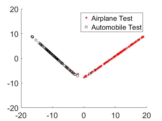
Figure 8 plots the representations for the selected airplane and automobile data from the CIFAR10 dataset. First, panels (a) and (b) show the features of the test set learned by ResNet56 visualized by the proposed two strategies. In both cases, the features are well separated, in general, with a small overlapping which causes some misclassification. Charts (c) and (d) depict the first two principal components (PCs) learned by ResNet56-WNLL for the selected training and testing data. The PCs of the features learned by ResNet56-WILL is better separated than that of ResNet56’s (Fig. 8), and it indicates that ResNet56-WILL is more accurate in classifying the randomly selected data.

5.2 Improving Adversarial Robustness

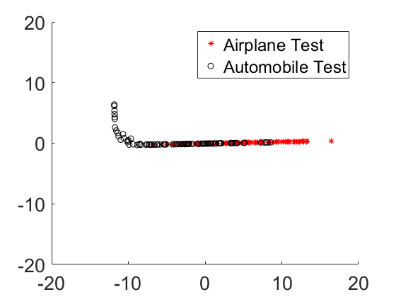
First, let us look at how the adversarial attack changes the geometry of the learned representations. We consider the simple one-step IFGSM attack, IFGSM¹, with the same parameters used before. Figure 9 shows the first two PCs of the representations learned by ResNet56 and ResNet56-WNLL for the adversarial test images. These PCs show that the adversarial attack makes the features of the two different classes mixed and therefore drastically reduces the classification accuracy.

Second, we consider how the WNLL interpolation helps to improve adversarial robustness. We randomly pick up an adversarial image that is misclassified by the standard DNNs with the softmax activation from the MNIST and the CIFAR10, respectively. The top five nearest neighbors in the deep feature space from the clean training data, of these two adversarial images, are shown in Fig. 10. For the MNIST digit, all the nearest neighbors belong to the same class as the adversarial image; and for the CIFAR10 adversarial image, the top three neighbors belong to the same category as the adversarial one. These nearest neighbors will guide DNN-WNLL to classify the adversarial images correctly.

6 Concluding Remarks

In this paper, we leveraged ideas from the manifold learning and proposed to replace the output activation function of the conventional deep neural nets (DNNs), typically the softmax function, with a graph Laplacian-based high dimensional interpolating function. This simple modification is applicable to any of the existing off-the-shelf DNNs with the softmax activation enables DNNs to make sufficient use of the manifold structure of data. Furthermore, we developed end-to-end and multi-staged training and testing algorithms for the proposed DNN with the interpolating function as its output activation. On the one hand, the proposed new framework remarkably improves both generalizability and robustness of the baseline DNNs; on the other hand, the new framework is suitable for data-efficient machine learning. These improvements are consistent across networks of different types and with a different number of layers. The increase in generalization accuracy could also be used to train smaller models with the same accuracy, which has great potential for mobile device applications.

In this work, we utilized a special kind of graph interpolating function as DNNs’ output activation. An alternative approach is to learn such an interpolating function instead of using one which is fixed. This approach is under our consideration.

Acknowledgments

This material is based on research sponsored by the Air Force Research Laboratory under grant numbers FA9550-18-0167 and MURI FA9550-18-1-0502, the Office of Naval Research under grant number N00014-18-1-2527, the U.S. Department of Energy under grant number DOE SC0013838, and by the National Science Foundation under grant number DMS-1554564 (STROBE).

References

Agostinelli et al. (2014) F. Agostinelli, M. Hoffman, P. Sadowski, and P. Baldi. Learning Activation Functions to Improve Deep Neural Networks. arXiv preprint arXiv:1412.6830, 2014.
Anonymous (2019) Anonymous. Adversarial Machine Learning against Tesla’s Autopilot. https://www.schneier.com/blog/archives/2019/04/adversarial_mac.html, 2019.
Athalye et al. (2018) A. Athalye, N. Carlini, and D. Wagner. Obfuscated Gradients Give a False Sense of Security: Circumventing Defenses to Adversarial Examples. In International Conference on Machine Learning, 2018.
Bengio et al. (2007) Y. Bengio, P. Lamblin, D. Popovici, and H. Larochelle. Greedy Layer-wise Training of Deep Networks. In Advances in neural information processing systems, 2007.
Brendel et al. (2017) W. Brendel, J. Rauber, and M. Bethge. Decision-based adversarial attacks: Reliable attacks against black-box machine learning models. arXiv preprint arXiv:1712.04248, 2017.
Carlini and Wagner (2016) N. Carlini and D.A. Wagner. Towards evaluating the robustness of neural networks. IEEE European Symposium on Security and Privacy, pages 39–57, 2016.
Chapelle et al. (2006) O. Chapelle, B. Scholkopf, and A. Zien. Semi-supervised Learning. Cambridge, Mass.: MIT Press, 2006.
Chen et al. (2017a) X. Chen, C. Liu, B. Li, K. Liu, and D. Song. Targeted Backdoor Attacks on Deep Learning Systems Using Data Poisoning. arXiv preprint arXiv:1712.05526, 2017a.
Chen et al. (2017b) Y. Chen, J. Li, H. Xiao, X. Jin, S. Yan, and J. Feng. Dual Path Networks. In Advances in neural information processing systems, 2017b.
Cohen et al. (2019) J. Cohen, E. Rosenfeld, and J. Z. Kolter. Certified Adversarial Robustness via Randomized Smoothing. arXiv preprint arXiv:1902.02918v1, 2019.
Dou et al. (2018) Z. Dou, S. J. Osher, and B. Wang. Mathematical Analysis of Adversarial Attacks. arXiv preprint arXiv:1811.06492, 2018.
Glorot et al. (2011) X. Glorot, A. Bordes, and Y. Bengio. Deep Sparse Rectifier Neural Networks. In Proceedings of the Fourteenth International Conference on Artificial Intelligence and Statistics, pages 315–323, 2011.
Goodfellow et al. (2013) I. Goodfellow, D. Warde-Farley, M. Mirza, A. Courville, and Y. Bengio. Maxout Networks. arXiv preprint arXiv:1302.4389, 2013.
Goodfellow et al. (2014) I. J. Goodfellow, J. Shlens, and C. Szegedy. Explaining and Harnessing Adversarial Examples. arXiv preprint arXiv:1412.6275, 2014.
Guo et al. (2018) C. Guo, M. Rana, M. Cisse, and L. van der Maaten. Countering Adversarial Images using Input Transformations. In International Conference on Learning Representations, 2018. URL https://openreview.net/forum?id=SyJ7ClWCb.
He et al. (2015) K. He, X. Zhang, S. Ren, and J. Sun. Delving Deep into Rectifiers: Surpassing Human-level Performance on Imagenet Classification. In Proceedings of the IEEE international conference on computer vision, pages 1026–1034, 2015.
He et al. (2016a) K. He, X. Zhang, S. Ren, and J. Sun. Identity Mappings in Deep Residual Network. In European conference on computer vision, 2016a.
He et al. (2016b) K. He, X. Zhang, S. Ren, and J. Sun. Identity Mappings in Deep Residual Networks. In European Conference on Computer Vision, 2016b.
He et al. (2016c) K. He, X. Zhang, S. Ren, and J. Sun. Deep Residual Learning for Image Recognition. In IEEE Conference on Computer Vision and Pattern Recognition, pages 770–778, 2016c.
Hinton et al. (2006) G. Hinton, S. Osindero, and T. Teh. A Fast Learning Algorithm for Deep Belief Nets. Neural Computation, 18(7):1527–1554, 2006.
Hinton et al. (2012) G. Hinton, N. Srivastava, A. Krizhevsky, I. Sutskever, and R. Salakhutdinov. Improving neural networks by preventing co-adaptation of feature detectors. arXiv preprint arXiv:1207.0580, 2012.
Huang et al. (2016) G. Huang, Y. Sun, Z. Liu, D. Sedra, and K. Weinberger. Deep Networks with Stochastic Depth. In European conference on computer vision, 2016.
Huang et al. (2017) G. Huang, Z. Liu, L. van der Maaten, and K. Weinberger. Densely Connected Convolutional Networks. In IEEE Conference on Computer Vision and Pattern Recognition, 2017.
Kingma and Ba (2014) D. Kingma and J. Ba. Adam: A Method for Stochastic Optimization. arXiv preprint arXiv:1412.6980, 2014.
Krizhevsky (2009) A. Krizhevsky. Learning Multiple Layers of Features from Tiny Images. 2009.
Krizhevsky et al. (2012) A. Krizhevsky, I. Sutskever, and G. Hinton. Imagenet Classification with Deep Convolutional Neural Networks. In Advances in neural information processing systems, pages 1097–1105, 2012.
Kurakin et al. (2017) A. Kurakin, I. Goodfellow, and S. Bengio. Adversarial Machine Learning at Scale. In International Conference on Learning Representations, 2017.
LeCun (1998) Y. LeCun. The MNIST Database of Handwritten Digits. 1998.
LeCun et al. (2015) Y. LeCun, Y. Bengio, and G. Hinton. Deep Learning. Nature, 521:436–444, 2015.
Lecuyer et al. (2019) M. Lecuyer, V. Atlidakis, R. Geambasu, D. Hsu, and S. Jana. Certified Robustness to Adversarial Examples with Differential Privacy. In IEEE Symposium on Security and Privacy (SP), 2019.
Li and Shi (2017) Z. Li and Z. Shi. Deep Residual Learning and PDEs on Manifold. arXiv preprint arXiv:1708.05115, 2017.
Liu et al. (2016) Y. Liu, X. Chen, C. Liu, and D. Song. Delving into transferable adversarial examples and black-box attacks. arXiv preprint arXiv:1611.02770, 2016.
Madry et al. (2018) A. Madry, A. Makelov, L. Schmidt, D. Tsipras, and A. Vladu. Towards Deep Learning Models Resistant to Adversarial Attacks. In International Conference on Learning Representations, 2018. URL https://openreview.net/forum?id=rJzIBfZAb.
Moosavi-Dezfooli et al. (2017) Seyed-Mohsen Moosavi-Dezfooli, Alhussein Fawzi, Omar Fawzi, and Pascal Frossard. Universal Adversarial Perturbations. In IEEE Conference on Computer Vision and Pattern Recognition, July 2017.
Muja and Lowe (2014) M. Muja and D. Lowe. Scalable Nearest Neighbor Algorithms for High Dimensional Data. Pattern Analysis and Machine Intelligence (PAMI), 36, 2014.
Nair and Hinton (2010) V. Nair and G. Hinton. Rectified Linear Units Improve Restricted Boltzmann Machines. In Proceedings of the 27th international conference on machine learning, pages 807–814, 2010.
Netzer et al. (2011) Y. Netzer, T. Wang, A. Coates, A. Bissacco, B. Wu, and A. Ng. Reading Digits in Natural Images with Unsupervised Features Learning. NIPS Workshop on Deep Learning and Unsupervised Feature Learning, 2011.
Osher et al. (2018) S. J. Osher, B. Wang, P. Yin, X. Luo, M. Pham, and A. Lin. Laplacian Smoothing Gradient Descent. arXiv preprint arXiv:1806.06317, 2018.
Papernot et al. (2016a) N. Papernot, P. McDaniel, S. Jha, M. Fredrikson, Z.B. Celik, and A. Swami. The Limitations of Deep Learning in Adversarial Settings. IEEE European Symposium on Security and Privacy, pages 372–387, 2016a.
Papernot et al. (2016b) N. Papernot, P. McDaniel, X. Wu, S. Jha, and A. Swami. Distillation as a Defense to Adversarial Perturbations Against Deep Neural Networks. IEEE European Symposium on Security and Privacy, 2016b.
Papernot et al. (2016c) Nicolas Papernot, Patrick D. McDaniel, and Ian J. Goodfellow. Transferability in Machine Learning: from Phenomena to Black-Box Attacks using Adversarial Samples. CoRR, abs/1605.07277, 2016c. URL http://arxiv.org/abs/1605.07277.
Paszke and et al (2017) A. Paszke and et al. Automatic Differentiation in PyTorch. 2017.
Ross and Doshi-Velez (2017) A. Ross and F. Doshi-Velez. Improving the Adversarial Robustness and Interpretability of Deep Neural Networks by Regularizing Their Input Gradients. arXiv preprint arXiv:1711.09404, 2017.
Samangouei et al. (2018) P. Samangouei, M. Kabkab, and R. Chellappa. Defense-GAN: Protecting Classifiers Against Adversarial Attacks Using Generative Models. In International Conference on Learning Representations, 2018. URL https://openreview.net/forum?id=BkJ3ibb0-.
Shi et al. (2018) Z. Shi, B. Wang, and S. Osher. Error Estimation of the Weighted Nonlocal Laplacian on Random Point Cloud. arXiv preprint arXiv:1809.08622, 2018.
Simonyan and Zisserman (2014) K. Simonyan and A. Zisserman. Very deep convolutional networks for large-scale image recognition. arXiv preprint arXiv:1409.1556, 2014.
Szegedy et al. (2013) C. Szegedy, W. Zaremba, I. Sutskever, J. Bruna, D. Erhan, I. Goodfellow, and R. Fergus. Intriguing Properties of Neural Networks. arXiv preprint arXiv:1312.6199, 2013.
Tang (2013) Y. Tang. Deep Learning Using Linear Support Vector Machines. ArXiv:1306.0239, 2013.
Tramèr et al. (2018) Florian Tramèr, Alexey Kurakin, Nicolas Papernot, Ian Goodfellow, Dan Boneh, and Patrick McDaniel. Ensemble Adversarial Training: Attacks and Defenses. In International Conference on Learning Representations, 2018. URL https://openreview.net/forum?id=rkZvSe-RZ.
Verma et al. (2018) V. Verma, A. Lamb, C. Beckham, A. Najafi, I. Mitiagkas, A. Courville, D. Lopez-Paz, and Y. Bengio. Manifold Mixup: Better Representations by Interpolating Hidden States. arXiv preprint arXiv:1806.05236, 2018.
Wan et al. (2013) L. Wan, M. Zeiler, S. Zhang, Y. LeCun, and R. Fergus. Regularization of Neural Networks Using Dropconnect. In International Conference on Machine Learning, pages 1058–1066, 2013.
Wang et al. (2018a) B. Wang, A. T. Lin, Z. Shi, W. Zhu, P. Yin, A. L. Bertozzi, and S. J. Osher. Adversarial Defense via Data Dependent Activation Function and Total Variation Minimization. arXiv preprint arXiv:1809.08516, 2018a.
Wang et al. (2018b) B. Wang, X. Luo, Z. Li, W. Zhu, Z. Shi, and S. Osher. Deep Neural Nets with Interpolating Function as Output Activation. In Advances in Neural Information Processing Systems, 2018b.
Wang et al. (2018c) B. Wang, B. Yuan, Z. Shi, and S. Osher. ResNets Ensemble via the Feynman-Kac Formalism to Improve Natural and Robust Accuracies. arXiv preprint arXiv:1811.10745, 2018c.
Zagoruyko and Komodakis (2016) S. Zagoruyko and N. Komodakis. Wide Residual Networks. In British Machine Vision Conference, 2016.
Zhang et al. (2019) H. Zhang, Y. Yu, J. Jiao, E. Xing, L. Ghaoui, and M. Jordan. Theoretically Principled Trade-off between Robustness and Accuracy. arXiv preprint arXiv:1901.08573, 2019.
Zheng et al. (2016) S. Zheng, Y. Song, T. Leung, and I. Goodfellow. Improving the Robustness of Deep Neural Networks via Stability Training. In IEEE Conference on Computer Vision and Pattern Recognition, 2016.