Trees, length spectra for rational maps via barycentric extensions and Berkovich spaces
Abstract.
In this paper, we study the dynamics of degenerating sequences of rational maps on Riemann sphere using -trees. As an analogue of isometric group actions on -trees for Kleinian groups, we give two constructions for limiting dynamics on -trees: one geometric and one algebraic. The geometric construction uses the limit of rescalings of barycentric extensions of rational maps, while the algebraic construction uses the Berkovich space of complexified Robinson’s field. We show that the two approaches are equivalent. As an application, we use it to give a classification of hyperbolic components of rational maps that admit degeneracies with bounded multipliers.
1. Introduction
The study of dynamics of rational maps has been a central topic in mathematics. The space of degree rational maps is not compact, so it is interesting and useful to understand the dynamics as rational maps degenerate. Let in . In [Luo19], we started the investigation of degenerating rational maps using the barycentric method. In particular, we constructed a limiting branched covering on -trees. The construction is done in steps (see §3 and §4):
- (1)
Using the barycentric extension, we first extend the rational map to .
- (2)
By choosing an appropriate rescalings
we get a limiting map on the ultralimit (also known as the asymptotic cone) of pointed metric spaces
Dynamics on -trees also arises naturally via Berkovich spaces (see [BR10, Kiw15]). Using the Berkovich space of the complexified Robinson’s field, we construct a limiting dynamical system on the -tree. This algebraic construction is done in steps as well (see §5 and §6):
- (1)
First we associate to the sequence a degree rational map with coefficients in the complexified Robinson’s field associated with the sequence .
- (2)
Using the Berkovich extension, the rational map naturally extends to a map on the Berkovich hyperbolic space,
We establish a connection between the two constructions:
Theorem 1.1.
There is a canonical isometric bijection
such that
Remark.
Both the asymptotic cone and the complexified Robinson’s field use non-principal ultrafilters in the construction. We remark that the same ultrafilter is used in both constructions.
We want to emphasize that each perspective of the limiting map brings its own unique advantages and benefits. The barycentric method allows us to work with degenerating sequence of conjugacy classes (see Theorem 4.2) and gives geometric information for the dynamics of . The Berkovich approach gives additional algebraic structure of the -tree.
The limiting dynamics of (or equivalently ) on the -tree is useful in recovering the limiting ratios of the length spectra for rational maps. Motivated by the theory of Teichmüller space and Kleinian groups, it is more natural to discuss length spectra for rational maps in a single hyperbolic component (cf. [MS98]), although most of the discussions also work without this assumption.
Markings and the length spectra.
A conjugacy class of a rational map is called hyperbolic if the orbit of every critical point converges to some attracting periodic cycle. The space of hyperbolic rational maps is open in the moduli space , and a connected component is called a hyperbolic component. For each hyperbolic component , there is a topological model
for the dynamics on the Julia set. That is, for any , there is a homeomorphism
which conjugates and . A particular choice of such will be called a marking of the Julia set.
Let be a hyperbolic rational map with a marking . Let be the space of periodic cycles of . We define the length of a periodic cycle for by
where and . The collection will be called the marked length spectrum of . As varies over the hyperbolic component, we aim to understand how the length spectrum changes. In particular, we will investigate the behavior of the length spectrum for a degenerating sequence via the limiting dynamics .
The ends of a tree and translation lengths
Let be an end of the tree . The translation length of an end measures the rate at which moves points of towards ; it is defined by
Let be a degenerating sequence with markings , and
Then (see Proposition 3.5), and we choose a sequence of representatives with
Let be the limiting map on . The markings give a marking on the ends of (see §9). If is a periodic cycle, then is a cycle of periodic ends. We define its translation length
It is a well-known principle that the translation lengths on the limiting -trees give information on the length spectrum (cf. [DM08, Luo19, McM09b, MS84]). The precise statement that we will prove and use is the following:
Theorem 1.2.
Let be degenerating with markings , and let be the associated limiting maps on . If is a periodic cycle, then
Moreover, every cycle of repelling periodic ends of is represented by some cycle .
Degeneracy with bounded length spectra.
Let be a hyperbolic component. It is natural to ask whether the marked length spectrum is a proper map on . In other words, is there a degenerating sequence with stays bounded for every ? Hence, we define
Definition 1.3.
A hyperbolic component is said to admit bounded escape if there exists a sequence with markings so that
- (1)
is degenerating;
- (2)
For any periodic cycle , the sequence of lengths is bounded.
Since there are only finitely many periodic points of a fixed period, we can formulate the definition without using the markings and replace the second condition by
- (2’)
For any and any sequence of periodic points of with period , the multipliers of at stay bounded.
We remark that the analogue of such a phenomenon cannot happen for degenerating Kleinian groups (cf. [MS84]), so it might already be surprising that such a hyperbolic component exists.
The first example comes from the McMullen family [McM88]. The sequence is contained in a hyperbolic component for all large , and the Julia set for this hyperbolic component is homeomorphic to a Cantor set of circles. In particular, any component of the Julia set separates the two points , , and the Julia set is disconnected. We will show these two topological characteristics of the Julia set classify all examples admitting bounded escape.
Definition 1.4.
Let be a hyperbolic rational map. We say is nested if
- (1)
There are two points such that any component of separates and ;
- (2)
contains more than one component.
A hyperbolic component is said to have nested Julia sets if the Julia set of any rational map in is nested.
Theorem 1.5.
A hyperbolic component admits bounded escape if and only if it has nested Julia sets.


In §10, we associate a combinatorial invariant to a hyperbolic rational map with nested Julia sets (see Proposition 10.4). We also show any such combinatorial data is realizable (see Theorem 10.6) (cf. [Luo20]). Using this, we prove nested Julia sets implies bounded escape.
To prove the other direction, from the definition, we have a degenerating sequence with bounded multipliers. This gives a limiting dynamics on an -tree with no repelling periodic ends. In §11, we classify such limiting dynamics and use our classification to derive topological properties of the Julia set. In the course of the proof, we also get a quantitative result: if is not nested, then there exists some periodic cycle whose multiplier escapes to infinity comparable to (see Theorem 11.13). We refer the readers to the discussion at the end of §11 for open questions.
Comparison with Kleinian groups
We conclude our discussion by comparing our results above with some well-known results for Kleinian groups.
- (1)
Hyperbolic components and markings. A hyperbolic component of rational maps is an analogue of , the space of conjugacy classes of discrete faithful representations of in . The repelling periodic cycles are in correspondence with the closed geodesics on the quotient hyperbolic 3-manifold. For Kleinian groups, closed geodesics are naturally marked by the representation. The markings of periodic cycles are, in general, not canonical.
- (2)
Limiting dynamics on -trees. In [MS84], based on the study of valuations on the function field of the character variety, Morgan and Shalen showed how to compactify using isometric actions on -trees, which shed new lights and generalized part of Thurston’s Hyperbolization Theorem. Bestvina and Paulin gave a more geometric perspective of this theory in [Bes88, Pau88]. In the rational map setting, the construction of limiting map on -trees using barycentric extensions is in the same spirit as Bestvina and Paulin’s construction, while the Berkovich dynamics, which studies valuations on polynomial rings, adapts the algebraic perspective as in Morgan and Shalen’s formulation. Theorem 1.1 is analogous to the equivalence of various constructions of -trees for Kleinian groups. We remark that the construction does not require the sequence to come from a single hyperbolic component in the rational map setting.
- (3)
- (4)
Bounded escape and nested Julia sets. These phenomena are new in the complex dynamics setting:
- •
A sequence in is degenerate if and only if the length of some closed geodesic escapes to infinity (see [MS84]).
- •
- •
- (5)
Blaschke products and Fuchsian groups/Teichmüller spaces. Under our dictionary, the space of Blaschke products is analogous to the space of Fuchsian representations. Our construction of dynamics on -trees is a direct generalization of the Ribbon -tree construction in [McM09b] for Blaschke products. We also refer to [McM08, McM09a, McM10] for more comparisons between Blaschke products and many other aspects of the Teichmüller spaces.
Notes and references
For more on -trees, degenerations of hyperbolic manifolds and rational maps, see e.g. [MS84, Bes88, Bes01, Pau88, Ota96, McM09b]. The use of asymptotic cone and the connection of -trees with the nonstandard analysis are developed and explained in [KL95, Chi91]. Other application of trees in complex dynamics can be found in [Shi89, DM08].
The use of Berkovich space of formal Puiseux series and rescalings to understand asymptotic behaviors for a degenerating holomorphic family of rational maps was introduced and made precise in [Kiw15]. Similar ideas have also been explored in [Sti93, Eps00, DeM07, Arf17]. In many situations, the study of parameter spaces leads us to consider sequences of rational maps. Our constructions of limiting maps on -trees, which use sequences, are usually better suited to answer such questions. For example, our theory easily gives a direct and uniform proof of the sequential version (compared to holomorphic family version) of the rescaling limit theorem in [Kiw15], and also allows us to eliminate the smoothness assumptions of the boundary when studying hyperbolic components in [NP20]. Other applications of Robinson’s field can be found in [dFM09].
Many examples of degenerating families of rational maps with bounded multipliers (Lattès family) without the hyperbolicity assumption are studied in [FRL10] using Berkovich dynamics. Rational maps with disconnected Julia sets are studied extensively in [PT00], and some examples of rational maps with nested Julia sets also appear there.
Acknowledgments
The author thanks C. T. McMullen for his advice and helpful discussion on this problem. The author gratefully thanks the anonymous referees for valuable comments and suggestions.
2. -trees and branched coverings
In this section, we give a brief introduction of -trees and set up some notations.
-trees.
An -tree is a nonempty metric space such that any two points are connected by a unique topological arc , and every arc of is isometric to an interval in .
We say is an endpoint of if is connected; otherwise is an interior point. If has three or more components, we say is a branch point. The set of branch points will be denoted . We say is a finite tree if is finite. We will write and for with one or both of its endpoints removed.
Ends and tangent vectors
A ray in the -tree is an isometric embedding of . We identify a ray as a map and its image in . Two rays are said to be equivalent if is still a ray. The collection of all equivalence classes of rays forms the set of ends of .
We will use to denote both a ray and the end it represents. We say a sequence of points converges to an end , denoted by , if for all , for all sufficiently large .
Let . Two segments and are said to represent the same tangent vector at if is non-degenerate segment. The set of equivalence classes of tangent vectors at is called the tangent space at , and denoted by . Equivalently, the tangent space can be identified with the set of components of .
Let . We will use to denote the component of corresponding to . More generally, if , we use to denote the component of with boundary .
Convexity and subtrees.
A subset of is called convex if . The smallest convex set containing is called the convex hull of , and is denoted by . More generally, we can easily extend the above definitions to subsets of .
Note that subset is convex is connected is a subtree. Moreover, is a finite subtree of is the convex hull of a finite set .
Branched coverings between -trees.
Let be a continuous map between two -trees, we say is a (tame) degree branched covering if there is a finite subtree such that
- (1)
is nowhere dense in , and is nowhere dense in .
- (2)
For every , there are exactly preimages in .
- (3)
For every , is a local isometry.
- (4)
For every , and any sufficiently small neighborhood of , is an isometric covering, where is the component of containing .
3. Barycentric extensions for rational maps
In this section, we briefly review the theory of barycentric extensions for rational maps. We will summarize some properties and refer the readers to [Luo19] for details.
The barycentric extension was extensively studied for circle homeomorphisms in [DE86]. The construction can be easily generalized to any continuous maps on the unit sphere , (see [Luo19, Pet11]). For our purposes, we will focus on the barycentric extensions for rational maps on , which is identified with under the stereographic projection.
We identify the hyperbolic space with the ball model . The conformal boundary of is naturally identified with in this way. A measure on is said to be balanced at a point if
where is any isometry sending to .
Given a probability measure on with no atoms of mass , there is a unique point , called the barycenter of , for which the measure is balanced (see [DE86, Hub06] or [Pet11]).
Let be the probability measure coming from the spherical metric on , and let be a non-constant rational map. The barycentric extension
is a map sending the point to the barycenter of the measure , where is any isometry sending to .
The extension is conformally natural: if , then
The following theorem concerning the regularities of the barycentric extensions is proved in [Luo19] (see Theorem 1.1 in [Luo19]):
Theorem 3.1.
For any rational map of degree , the norm of the derivative of its barycentric extension satisfies
Here the norm is computed with respect to the hyperbolic metric, and is a universal constant.
The space of rational maps
The space of rational maps of degree is an open variety of . More concretely, fixing a coordinate system of , then a rational can be expressed as a ratio of homogeneous polynomials , where and have degree with no common divisors. Using the coefficients of and as parameters, then
where is the vanishing locus for the resultant of and .
The space is not compact. A sequence is said to be degenerating, denoted by , if escapes every compact set of . One natural compactification of is .
Every map in determines the coefficients of a pair of homogeneous polynomials, and we write
where and is a rational map of degree at most . A zero of is called a hole of and the set of zeros of is denoted by . We define the degree of as the degree of .
The limit map describes the limiting dynamics away from the holes (see Lemma 4.2 in [DeM05]):
Lemma 3.2.
Let converge to . Then converges compactly to on .
Note that if converges to a degree map, the measure converges weakly to a delta measure. So the image of
On the other hand, if converges to with , converges weakly to , so
Therefore, we have the following proposition (see Proposition 5.5 in [Luo19]):
Proposition 3.3.
Let . Then is uniformly bounded if and only if degree maps are not in the limit set of in .
The following proposition gives a criterion for degeneracy (see Proposition 8.1 in [Luo19]):
Proposition 3.4.
Let , and . Then is degenerating if and only if .
The moduli space of rational maps.
The group of Möbius transformations acts on by conjugation. The quotient space is known as the moduli space of rational maps. A sequence is said to be degenerating, denoted by , if escapes every compact set of . Equivalently, if and only if every sequence of representatives is degenerating.
Since choosing a base point is equivalent to choosing a representative of the conjugacy class up to the compact group , we define
The following proposition follows immediately from the definition and Proposition 3.4 (see also Proposition 8.10 in [Luo19]):
Proposition 3.5.
The sequence in if and only if .
4. Ultralimits and asymptotic cones
In this section, we will review a standard construction of ultralimits for sequences of pointed metric spaces. The construction uses a non-principal ultrafilter, which is an efficient technical device for simultaneously taking limits of all sequences without passing to subsequences and putting them together to form one object. We refer the readers to [Gro92, KL95, Roe03] for more details.
Ultrafilters on .
We begin by reviewing the theory of ultrafilter on . A subset of the power set of is called an ultrafilter if
- (1)
If , then ;
- (2)
If and , then ;
- (3)
;
- (4)
If , then either or
By virtue of the above properties, one can think of an ultrafilter as defining a finitely additive -valued probability measure on . The sets of measure are precisely those belonging to the ultrafilter .
We will call a set in as -big or simply big. Its complement is called -small or simply small. If a specific property is satisfied by a -big set, we will also say this property holds -almost surely.
Let . We can construct an ultrafilter by
Any ultrafilter of the above type is called a principal ultrafilter. It can be verified that an ultrafilter is principal if and only if it contains a finite set. An ultrafilter that is not principal is called a non-principal ultrafilter. The existence of a non-principal ultrafilter is guaranteed by Zorn’s lemma.
Let be a non-principal ultrafilter on . Let be a sequence in a metric space and . We say is the -limit of , denoted by
if for every , the set is -big.
It can be easily verified (see [KL95]) that
- (1)
If the -limit exists, then it is unique.
- (2)
If is contained in a compact set, then the -limit exists.
- (3)
If in the standard sense, then .
- (4)
If , then there exists a subsequence such that in the standard sense.
From these properties, one should think of the non-principal ultrafilter as performing all the subsequence-selection in advance. All sequences in compact spaces will automatically converge without the need to pass to any further subsequences.
From now on and throughout the rest of the paper, we will fix a non-principal ultrafilter on .
Ultralimit of pointed metric spaces.
Let be a sequence of pointed metric spaces with basepoints . Let denote the set of sequences such that is a bounded function of . We also define an equivalence relation by
We use to denote the equivalence class of the sequence .
Let , and we define
The function makes a metric space, and is called the ultralimit of with respect to the ultrafilter , and is written as or simply for short.
Asymptotic cones of .
Given a positive sequence , we define the asymptotic cone with rescaling as the ultralimit
From the definition, a point is represented by a sequence with , and .
Ends of .
Let , viewed as a point on the conformal boundary of . We denote as the point of distance from in the direction of . Given any sequence , the ray
is a geodesic ray parameterized by arc length in . Thus, corresponds to an end . We denote this by .
Limiting map on .
Let be a degenerating sequence of rational maps. The appropriate rescaling to use is
as it brings all the preimages of in view. Let be the asymptotic cone of with respect to the rescaling .
The limiting map is defined by
Since all are -Lipschitz by Theorem 3.1 with a universal constant , it follows that is well defined. In [Luo19], we showed that the limiting map is a degree branched covering (see Theorem 1.2 in [Luo19]):
Theorem 4.1.
Let in , with . Then the limiting map
is a degree branched covering of the -tree .
Degenerating sequences in .
Let in . Recall that by Proposition 3.5, we have
We can choose representatives so that
The following theorem is the version for (see Theorem 8.11 in [Luo19]):
Theorem 4.2.
Let in and . Let be a representative of with
Then the corresponding limiting map
is a branched covering of degree with no totally invariant point.
5. Rational maps on Berkovich projective space
In this section, we give a brief review of the Berkovich projective space for a complete, algebraically closed non-Archimedean field , and the dynamics of rational maps on it. We refer the readers to [BR10] for a more detailed exposition of this theory.
Let be a complete, algebraically closed non-Archimedean field. We use and to denote the closed ball and open ball centered at with radius respectively. Recall that in a non-Archimedean field, any point (or ) is the center. If two balls intersect, then one is contained in the other.
The valuation ring of will be denoted as , and its maximal ideal is . The residual field is .
Let be a rational map with coefficients in . After multiplying the denominator and numerator by a common factor, we may assume that the maximum norm of the coefficients is . The reduction map is given by taking the reduction on its coefficients.
The Berkovich affine space and the Berkovich projective space
As a topological space, can be defined as follows. The underlying point set is the collection of all the multiplicative seminorms on the polynomial ring which extend the absolute value on . The topology on is the weakest one for which is continuous for all . The field can be thought of as a subspace of , via the evaluation map. That is, we can associate to a point the seminorm
The seminorms of this form will be called classical points.
The Berkovich projective space is the one point compactification of . The extra point, which is denoted, as usual, by , can be regarded as the point embedded in .
Berkovich classification.
Given closed ball , one can construct the supremum norm
One of the miracles of the non-Archimedean universe is that this norm is multiplicative. More generally, given any decreasing sequence of closed balls , we can consider the limiting seminorm
Berkovich’s classification asserts that every point arises in this way, and we can classify them into types:
- (1)
Type I: Points in , which we will also call the classical points;
- (2)
Type II: Points corresponding to a closed ball with ;
- (3)
Type III: Points corresponding to a closed ball with ;
- (4)
Type IV: Points corresponding to a nested sequence with empty intersection.
Type I, II and III can all be thought of a special case of Type IV: the classical points correspond to a nested sequence with ; the Type II points correspond to a nested sequence with nonempty intersection and belongs to the value group ; the Type III points correspond to a nested sequence with nonempty intersection but does not belong to the value group .
We will call the point corresponding to the gauss point and is denoted by .
Rational maps on
There is a ‘Proj’ construction of , which allows us to extend the natural action of on to , preserving the types of the points (see §2 in [BR10]).
Given any Type II point , there exists such that . We will regard as a ‘change of coordinates’. For our purposes, we can treat the following proposition as the definition of rational maps on Type II points (see Lemma 2.17 in [BR10]).
Proposition 5.1.
Let , and let be Type II points. Assume that and with . Then if and only if has non-constant reduction.
The tree structure on .
The Berkovich hyperbolic space is defined by
Note that is also the space of Type II, III and IV points.
Given two Type II or III points corresponding to the balls and respectively, we let be the smallest ball containing both and . Note that . We define the distance function
Note that if is contained in , then
which should be interpreted roughly as the modulus of the open annulus . In general, the distance is the sum of modulus of and .
One can extend this distance formula continuously to arbitrary points . The metric space can be shown to be a complete -tree (see Proposition 2.29 in [BR10]). Moreover, the finite ends of the -tree correspond to the Type IV points, while the infinite ends of the -tree correspond to the classical (Type I) points. The group acts isometrically on which is transitive on Type II points.
We remark that the topology generated by the metric is strictly finer than the subspace topology of the Berkovich topology on . In this paper, we shall mainly use the topology generated by this metric.
Tangent maps and multiplicities.
The tangent space at is the space of components of . If is the Gauss point, the tangent space is identified with the projective line of the residual field . More generally, if is a Type II point, we can choose so that . The isometry allows us to identify with .
If , then induces a natural tangent map
The following theorem follows from Corollary 9.25 in [BR10]:
Theorem 5.2.
Let be a Type II point, and . Choose so that and . Let , and let be the reduction of . Then under the identification of (and ) with by (and respectively), the tangent map equals to the reduction map .
There are many equivalent ways to extend the definition of local degrees for from to in the literature (see §2 in [FRL10] and Chapter 9 in [BR10]). Theorem 5.2 allows us to define it for Type II points. Let be a Type II point. We define the local degree
If we now count each point by its multiplicities, then every point has exactly preimages in .
6. Complexified Robinson’s field
In this section, we study a complete, algebraically closed, non-Archimedean field . This field is first introduced in the real setting by Robinson to formulate the non-standard analysis.
Recall that is a fixed non-principal ultrafilter . Let be the set of all sequences in . We say two sequence and are equivalent if
The set of equivalence classes will be denoted by .
The addition and multiplication are defined naturally: if are represented by and , then and are the class represented by and . It can be checked that these are indeed well defined and make a field. This field is usually referred to as the ultrapower construction for (cf. Chapter 2 in [LR75]).
Given represented by and , we write or if or -almost surely.
The field is usually too big to work with in our applications and is not equipped with a norm. We will construct a more useful field as the quotient of a subspace of .
Let be a positive sequence, which is regarded as . With the notations above, we construct
and
We remark that since , consists of those (equivalence classes of ) sequences that are not growing to infinity too fast, while consists of those tending to very fast. It is easy to show that both and form rings with respect to the addition and multiplication of . It can also be shown that is a maximal ideal of ring (cf. Chapter 3.3 in [LR75]). We define
as the quotient field. Note that embeds into via constant sequences.
Intuitively, the field lies in between and consisting of those large infinitesimals and small infinite numbers. We shall regard each member of as a small infinitesimal, and its multiplicative inverse (provided that ) a large infinite number.
We can define an equivalence relation on : if . Note that if , then if and only if as a member of .
Non-Archimedean norm on
One of the many desired properties of is that we can put a norm on it. Let and represented by and respectively. Note that there exist two integers such that , hence the ultralimit
is a finite number. Note that
Since , . Hence .
Therefore, we have a well-defined valuation for by
where is a representative of .
Notice that by definition, . More generally, .
To simplify the notations, from now on, we will use a single roman letter to represent a number in , and drop the square bracket.
It can be easily verified that for (cf. Chapter 3 Lemma 3.1 and 3.2 in [LR75]), we have
Hence, defines a non-Archimedean valuation on , and this valuation naturally gives rise to a non-Archimedean norm via
The distance function is given by
The field is spherically complete
A metric space is said to be spherically complete if for any nested sequence of (closed) balls , their intersection is non-empty. We show:
Theorem 6.1.
The field is spherically complete.
Proof.
Let be a decreasing sequence of closed balls. We consider a decreasing sequence of open balls so that . We assume that has radius , and denote . Pick , and assume that is represented by . Since for all , we know
Equivalently,
We can construct inductively a decreasing sequence such that
- (1)
is -big;
- (2)
;
- (3)
For any and , we have
Indeed, we can set as the base case. Assume that is constructed. To construct , we note that for any ,
Hence, there exists an -big set so that for all and ,
We define , then is still -big. Property is satisfied by the induction hypothesis and by the definition of . Property holds as by construction.
We now define the sequence for , and let . Note that for any , by Property , for some . Hence for any and ,
Therefore, . This means that , so .
Since this holds for any , we conclude that , so . Therefore, as well. ∎
As an immediate corollary, we have (cf. Chapter 3 Theorem 4.1 in [LR75]):
Corollary 6.2.
The field is complete.
The field is algebraically closed
We will show that not only does have good completion properties, it is also algebraically closed.
Theorem 6.3.
is algebraically closed.
Proof.
Let be a monic polynomial with coefficients . We assume that . Hence there is an -big set so that for all and ,
Now let and . Note that for any , on the circle centered at of radius (note that as ) that
By Rouché’s theorem, there are solutions of in the ball . Let be such a root. Note that is defined on an -big set , so represents a point in as for all . Moreover, satisfies the equation . Therefore, is algebraically closed. ∎
Since the value group of is , as an immediate corollary of the previous two theorems and the Berkovich classification theorem, we have
Corollary 6.4.
The Berkovich hyperbolic space consists of only Type II points.
The residue field of
For the complexified Robinson’s field , each non-zero element in can be represented by a sequence with
Two sequences and represent the same element in if . Thus, the field embeds into the residual field by taking constant sequence.
Embedding of the field of Puiseux series
In this subsection, we will show how to embed the field of formal Puiseux series into the Robinson’s field (cf. Chapter 3 §6 in [LR75]).
The field is the algebraic closure of the completion of the field of formal Laurent series . An element in can be represented by a formal series
where , so that if does not vanish for sufficiently large , then as . The absolute value is given by
provided .
To show we have an embedding, we first prove the following lemma about the convergence of series in .
Lemma 6.5.
Let , and be an unbounded increasing sequence of . Then the series
converges in .
Moreover, .
Proof.
Let . If , then . Otherwise, . Since , so . Hence, the series converges in by the convergence criterion in non-Archimedean field.
For the moreover part, let be the associated partial sums. Without loss of generality, we assume that , then for all by the strong triangle inequality. Therefore . ∎
Let . We define as follows.
Note that the series converges by Lemma 6.5. One can easily verify that and . Hence we have
Proposition 6.6.
The map
is an embedding of fields and preserves the non-Archimedean norms.
7. Equivalence of barycentric and Berkovich construction
In this section, it is better to use the upper space model of the hyperbolic -space . We can identify , and a linear map extends to an isometry on given by
| (7.1) |
The distance between two points and is given by the formula
| (7.2) |
We will identify as the point .
Construction of the isometric bijection .
By Corollary 6.4, consists of only Type II points. Hence by the Berkovich classification theorem, every point can be represented by a closed ball . We consider a linear polynomial of the form
with . Representing and by the sequences and , we get a sequence of Möbius transformations
Let be the asymptotic cone of with respect to rescaling . We define
Proposition 7.1.
is a well-defined isometric bijection.
Proof.
We will first check that this definition is well defined. Let be a different representation, where represent and . Since , and . Without loss of generality, we assume -almost surely.
Let . By definition of the norm on ,
- (1)
, -almost surely;
- (2)
, -almost surely.
Rearranging the inequalities and using the fact that , we have,
- (1)
, -almost surely;
- (2)
, -almost surely.
Consider , then using equations 7.1 and 7.2, we conclude that on an -big set,
Since is arbitrary, we conclude and represent the same point in . Therefore, is a well-defined map.
We will now show that is bijective. To show this, we will construct the inverse map . Given a point , we can represent it as , where . Using equations 7.1 and 7.2, we conclude that and for some -almost surely. Hence represent , with . Denote , and we define
Similarly, we can easily check that is well defined, and , are identity maps. Therefore is bijective.
We will now show that is an isometry. Given represented by and , then and where are isometries of and respectively. Hence, it suffices to show .
If is represented by a closed ball either contained or containing , then we can choose , and . A direct computation using equation 7.2, we have , so
where the last equality holds by the definition of norm on .
More generally, if is represented by a closed ball disjoint from , one can construct a geodesic by connecting to and then connecting to . By the above argument, one can show that is an isometry on either geodesic segment. Since is a bijection, and is a tree, this means . Therefore, is an isometry. ∎
The isometric bijection is a conjugacy.
Before proving the equivalence theorem, we need the following algebraic lemma.
Lemma 7.2.
Let , and be a sequence representing . Let be the limiting map on . Then the reduction of has degree if and only if .
Proof.
If the reduction of has degree , we can represent
with and . We denote
where and represent and in .
Let be the largest index so that
for all . Similarly, we define accordingly.
If , we let , then
has degree . Since , by Proposition 3.3,
Since , by equations 7.1 and 7.2, for any
for all large . Hence we have .
We are now ready to prove a more precise version of Theorem 1.1:
Theorem 7.3.
Let in . Let be the asymptotic cone with respect to the rescalings , and be the complexified Robinson’s field with respect to . Then represents a rational map , and
where is the limiting map on , and is the Berkovich extension of on .
Conversely, if , and for (any) sequence representing , we have
Proof.
Write so the maximum of and is . Thus, the sequences of coefficients , represent elements in . Let be the corresponding rational map with coefficients in . Note that a priori, the degree of may be .
Let be the map defined as above. Then is an isometric bijection. Given represented by the sequence where . Assume that is represented by where . Let be represented by and respectively. Then by naturality of the barycentric extension and Lemma 7.2, the reduction
has degree . By Proposition 5.1 and the definition of , . Hence is a conjugacy between and .
Since has degree by Theorem 4.1, we conclude has degree as well. Therefore, has degree , so .
The converse part follows by a similar argument. ∎
A version of holomorphic families.
Let be a holomorphic family of rational maps of degree defined over the punctured unit disk . We also assume that all the coefficients of extend to meromorphic functions on the unit disk . We may view as a rational map with coefficients in the field of formal Puiseux series .
Theorem 7.4.
Let and . There is an isometric embedding
Moreover, if is a holomorphic family of rational maps of degree defined over , then
where is the limiting map on , and is the Berkovich extension of on .
Proof.
By Proposition 6.6, the field naturally embeds isometrically into . Such an embedding gives an isometric embedding of into by the Berkovich classification theorem. A rational map with coefficients in can be thought of as a rational map with coefficients in via the embedding. Its action on naturally extends to . The theorem now follows from Theorem 7.3. ∎
8. Properties of the limiting map
In this section, using the equivalence result proved in Theorem 1.1 and Theorem 7.3, we summarize some properties of that will be used later.
Expansion and local degrees.
Recall that the local degree is the degree of the reduction of , where , and represent . The local degree in the direction , denoted by , is defined as the degree of at .
The following theorem allows us to interpret the local degree quite concretely as a local expansion factor (see Proposition 3.1 in [RL05], Theorem 9.26 in [BR10] and Theorem 4.7 in [Jon15]).
Theorem 8.1.
Let , and .
- (1)
For all sufficiently small segment representing , maps homeomorphically to and expands by a factor of .
- (2)
If , and are the preimages of in , then
If is an end associated to , then for all sufficiently large , maps homeomorphically to and expands by a factor of .
Approximating disks and annuli
We say a sequence of simply connected domains approximates an open disk if
- (1)
any sequence represents a point in the closed disk ;
- (2)
any sequence represents a point in .
Similarly, we say a sequence of annuli approximate an open annulus if
- (1)
any sequence represents a point in ;
- (2)
any sequence represents a point in .
The following lemma gives the classification for approximating disks and annuli. To distinguish the disks in and , we use to represent an open disk centered at with radius in .
Lemma 8.2.
Let be an open disk. A sequence of simply connected domains approximates if and only if
for all .
Let be an open annulus. Denote . A sequence of annuli approximates if and only if
for all , .
Proof.
To simplify the notations, all the statements below are assumed to hold -almost surely. Assume approximates . Suppose for contradiction that . Let . Then represents a point in . Since approximates , represents a point in . This is a contradiction. Thus, . Similarly, .
Conversely, assume for all . Let . Then represents a point . Indeed, otherwise, let with . Then contradicting to the assumption. Similarly, any sequence represents a point in . So approximates .
The proof for the annulus is similar. ∎
Recall that for , is the component associated to . By identifying with , is identified with an open disk . We say a sequence of simply connected domains approximates if after changing coordinates, and approximates .
Given two points , there is a unique component of with boundary . We can identify it with an open annulus . We define a sequence approximates in a similar way.
Remark.
We remark that if approximate , then the modulus satisfies
In particular, the sequence of moduli goes to infinity.
Limiting dynamics on disks and annuli
It is important to understand how the limiting map acts on and . We first define a critical end as an end of associated with a critical point in . The critical tree is defined as the convex hull of the critical ends. Since the residual characteristic of is , any point not in the critical tree has local degree (see Lemma 4.12 in [Jon15], or [Fab13a, Fab13b]). The following lemma follows from from Theorem 9.42, Theorem 9.46 in [BR10] and the above observation.
Lemma 8.3.
- (1)
Let , and . Assume that does not intersect the critical tree . Then is an isometric bijection from to .
- (2)
Let , and , . Assume that contains no critical ends. Then is a branched covering map from to .
Let and be as in the above lemma. Since contains no ends associated with critical values. We can choose a sequence approximating which contains no critical values of . Then is a union of annuli by Riemann-Hurwitz formula. Note that if the sequence represents , then represents . Thus, after changing the subindices, by Lemma 8.2, approximates . Therefore, by the Lemma 8.3, we have
Lemma 8.4.
Let , and , . Assume that contains no critical ends, so is a degree branched covering. Then there exist sequences of annuli and approximating and such that
is a degree covering -almost surely.
Extension on geodesic segments.
The following lemma allows us to extend the tangent map to geodesic segments (see Lemma 9.38 in [BR10]):
Lemma 8.5.
Let , and . Let . Then there exists such that maps homeomorphically to .
9. Marked length spectra and periodic ends
In this section, we shall illustrate how to use the limiting dynamics on -trees to study the marked length spectra of rational maps.
Markings and Length Spectra.
Recall that a conjugacy class of a rational map is hyperbolic if any of the following equivalent definition holds (see Theorem 3.13. in [McM94]):
- (1)
The postcritical set is disjoint from the Julia set .
- (2)
There are no critical points or parabolic cycles in the Julia set.
- (3)
Every critical point of tends to an attracting cycle under forward iteration.
- (4)
There is a smooth conformal metric defined on a neighborhood of the Julia set such that for all .
- (5)
There is an integer such that strictly expands the spherical metric on the Julia set.
The space of hyperbolic rational maps is open in , and a connected component is called a hyperbolic component. For each hyperbolic component , there is a topological dynamical system
such that for any , there is a homeomorphism
which conjugates and . A particular choice of such will be called a marking of the Julia set.
Let be a hyperbolic rational map with a marking . Let be the space of periodic cycles of the topological model . We define the length of a periodic cycle for by
where and . The collection will be called the marked length spectrum of .
Markings of periodic ends.
Let be a degenerating sequence with markings . Recall that we have
where is a representative of . We choose a sequence of representatives of so that
Let be the limiting map on the asymptotic cone with rescalings . The sequence of markings naturally gives a map by
Note that if is a periodic point of period , then for all . Hence, is a periodic point of represented by . Therefore, by Theorem 1.1, a periodic cycle is identified via with a cycle of periodic ends of for .
Translation length on ends.
Let represent an end. We will first show that the translation length
is well defined.
If is not a critical end, then by Theorem 8.1, is an isometry on for a sufficiently large . Hence is constant for , so the translation length is well defined.
If is a critical end, then by Theorem 8.1, is expanding with derivative on for a sufficiently large . Hence,
for all , so the translation length
If is a cycle of periodic ends, we define
We say a periodic end is attracting, indifferent or repelling if or .
Using the equivalence result in Theorem 1.1, we give an algebraic proof of Theorem 1.2 (cf. Theorem 1.4 in [Luo19]):
Proof of Theorem 1.2.
By considering iterations if necessary, we may assume has period . By naturality, we may also assume for all . Let be represented by . Note that .
We first claim that is not a critical point of . Indeed, since , , so . Hence, we can write
with and .
Let be and . Note that if is sufficiently small,
has non-constant reduction. Hence, we conclude that sends to where and represent and respectively. Therefore, the translation length is
By choosing representatives, we have
Thus, the result follows.
To show the moreover part, we note that any periodic point not in the Julia set is non-repelling. The multiplier has bounded norm. Hence . But the total number of periodic points of period for is the same as that of , so all repelling periodic points of are represented by periodic points in the Julia sets. Therefore, every cycle of repelling periodic ends is represented by some . ∎
Since the ultralimit of a sequence of real numbers belong to its limit set , by choosing subsequences and a diagonal argument, we immediately have
Corollary 9.1.
Let be a degenerating sequence, and be defined as above. Then after possibly passing to subsequences, we have
10. Hyperbolic components with nested Julia sets
In this section, we will study a special type of hyperbolic components. Recall that a hyperbolic rational map has nested Julia set if
- (1)
There are two points such that any component of separates and ;
- (2)
contains more than one component.
A hyperbolic component is said to have nested Julia sets if the Julia set of any rational map in is nested.
We remark that has uncountably many components by taking preimages and their accumulation points. The first example of hyperbolic rational map with nested Julia sets was introduced by McMullen in [McM88], where the Julia set is homeomorphic to a Cantor set times a circle.
Topological properties
We begin by introducing some terminologies and deducing some topological properties of the Julia set.
Let be a hyperbolic rational map with nested Julia sets, and be its Julia set. Since each component of separates points , any Fatou component of is either simply connected, or is isomorphic to an annulus. We will call a simply connected Fatou component a disk Fatou component, and an annulus Fatou component a gap. A gap is called critical if it contains critical points of .
We say a Julia component of is
- •
extremal if is contained in a component of ;
- •
buried if does not intersect the boundary of any Fatou component;
- •
unburied if it is not buried.
We first verify the following basic topological properties.
Lemma 10.1.
Let be a hyperbolic rational map with nested Julia sets . Then
- (1)
The gaps are nested, backward invariant, and any gap is eventually mapped to a disk Fatou component.
- (2)
Any non-extremal periodic Julia component is buried.
- (3)
Any unburied Julia component is eventually mapped to an extremal Julia component by a degree covering.
- (4)
Any buried Julia component is a Jordan curve.
- (5)
A critical gap is mapped to a disk Fatou component whose boundary is contained in an extremal Julia component.
- (6)
The extremal Julia components are mapped to extremal ones.
Proof.
Since the Julia set is nested, the gaps are nested. Since no disk Fatou component is mapped to a gap, they are backward invariant. Let be a periodic Fatou component. Since is hyperbolic, is attracting. Thus, contains a critical point of the first return map . By Riemann-Hurwitz formula, is a disk Fatou component. By no wandering domain theorem, every Fatou component is pre-periodic, so the statement (1) follows.
Let be a periodic Julia component of period . By conformal surgery (see Proposition 6.9 in [McM88]), there exists a post-critically finite hyperbolic rational map so that is conjugate to .
If is not extremal, then exactly two components of intersects . Thus, the two corresponding components of are totally invariant under , so is conjugate to either or for some . Hence is a Jordan curve. Since is not extremal, does not intersect the boundary of a disk Fatou component. The component does not intersect the boundary of a gap either, as otherwise, we would have a periodic gap. Thus is buried, and the statement (2) follows.
Since unburied Julia components are pre-periodic by no wandering domain theorem, and the image of an unburied Julia component is unburied, the statement (3) follows from (2).
By Theorem 1.2 in [PT00], any wandering component of is a Jordan curve. Since extremal components are not buried, and any non-extremal periodic Julia component is a Jordan curve, the statement (4) follows.
By Riemann-Hurwitz formula, critical gaps are mapped to disk Fatou components. Let be a critical gap, and be two components of the Julia set containing . Note is a Julia component. We claim is an extremal Julia component. Otherwise, exactly two components of intersect . Since is mapped to a disk Fatou component, the induced surjective map between ideal boundaries of and sends the ideal boundary corresponding to in to (cf. §6 in [McM88]). Thus there are at least 3 components of intersecting , which is a contradiction and the statement (5) follows.
A similar argument also shows that the extremal Julia components are mapped to extremal ones, giving the statement (6). ∎
Shishikura tree for nested Julia sets
We shall see that the dynamics on the gaps for a hyperbolic rational map with nested Julia sets is captured by the Shishikura tree. The Shishikura tree was first introduced by Shishikura in [Shi89] to study Herman rings. We will briefly introduce the special case that we are interested in, and refer the readers to [Shi89] for details and more general theories.
Let be an annulus of with modulus . Then there is a conformal map unique up to post composing with rotation sending the inner boundary to the inner one, and outer to the outer one. We define
Note that is a sub-annuli of .
Let be a hyperbolic rational map with nested Julia sets of degree , and let be the collection of gaps. Since the union of gaps is contained in the annulus bounded by the two extremal Julia components, which has finite moduli, by Grötzch inequality, . We define a pseudo metric on by
In the usual fashion, we identify two points if .
Note that if are in the same component of , then . More generally, the annulus is foliated by Jordan curves , and any two points have distance . Thus, the quotient is constructed by collapsing complementary components and leaves in the foliation. Since the annuli in the collection are nested, is isometric to a closed interval , and we denote
as the projection map.
The dynamics of on determines an associated map on via
where is the boundary of . By Theorem 3.6 in [Shi89], is well defined and continuous. We will now prove some properties of the map .
Lemma 10.2.
Let . Then there exist such that
- (1)
is a linear isometry with derivative ;
moreover, and the signs alternating;
- (2)
is a critical gap if and only if ;
moreover, ;
- (3)
, and .

Proof.
Consider the annulus . The boundary equals to the two extremal Julia components. Since the Julia set is nested, each component of is an annulus. Let be the projection of the boundary . We get .
Let . Since , each . Now restricting to and , then . The map is a degree covering, so restricting to is linear with derivative . This is true for any such , so is a linear on with derivative .
Since the critical gap is mapped to a simply connected Fatou component whose boundary is contained in the extremal Julia component, and all the other gaps are mapped to other gaps, the property follows immediately.
For the last property, we note that the gaps are backward invariant. Hence if we pick an arbitrary gap, there are exactly preimages counted multiplicities. Therefore .
Note that . If , then by the equality case of the Grötzch inequality (see Theorem B.5 in [McM94]), and share a Jordan curve boundary . Since , we can choose simple closed curves and with . Then has a critical point bounded between and , so has a critical point on . This is a contradiction as and is hyperbolic, so . ∎
Let , and be the set of periodic points in . By Proposition 10.2, is a Cantor set and .
Corollary 10.3.
The restriction on gives a surjective continuous map with connected fiber. Moreover, the repelling periodic points of are contained in .
Proof.
Since is a semi-conjugacy, it is easy to verify that . Hence is surjective and continuous. The fiber is connected as otherwise, contains a gap which is a contradiction. The moreover part follows directly from the fact is a semi-conjugacy. ∎
Let . Switching and , and take the second iteration of if necessary, we may assume that . Note if is even, then , and if is odd, then .
Recall that is called a polynomial like map if is a proper holomorphic map, and . The degree of a polynomial like map is defined as the degree of the proper map. The filled Julia set of the polynomial like map is defined as . If is connected, then is quasiconformally conjugate (in fact, hybrid conjugate) to a polynomial of the same degree, which is unique up to affine conjugation.
For sufficiently small , we have
Let and . Since , are open sets with and is proper of degree . Hence, is a polynomial like map, with connected filled Julia set . Let be the conjugate polynomial. Then is hyperbolic with connected Julia set as is hyperbolic. Similarly, if , then we can associate a hyperbolic polynomial with connected Julia set to the end .
Note that if varies in the hyperbolic component, (or ) also varies in the corresponding hyperbolic component of polynomials. Hence, combining Lemma 10.2, we summarize the invariants that we can associate to a hyperbolic component with nested Julia sets in the following proposition.
Proposition 10.4.
Let be a hyperbolic component with nested Julia sets in , and . Taking the second iteration if necessary, we assume that fixes (at least) one of the two extremal Julia components. We can associate the following set of invariants to :
- (1)
A natural number , and a sequence such that , and , where these numbers are associated to as in Lemma 10.2.
- (2)
If is even, a hyperbolic component with connected Julia set;
- (3)
If is odd, two hyperbolic components , with connected Julia set.
Next, we shall see that given any set of data as above, one can construct a hyperbolic component with nested Julia sets with that set of data as invariants. We emphasize that this set of invariants, however, is not complete: different hyperbolic components may share the same invariant. We refer the readers to [Luo20] for a complete invariant.
Construction of hyperbolic component with nested Julia sets.
In this subsection, we will use quasiconformal surgery to construct examples of nested Julia sets. We start by reviewing some of the definitions.
Let . Let , and set . A map is called -quasiconformal if
- (1)
is a homeomorphism;
- (2)
the partial derivatives and exist in the sense of distributions and belong to (i.e. are locally square integrable);
- (3)
and satisfy in .
A map is called -quasiregular if , where is quasiconformal and is holomorphic.
The following fundamental lemma for quasiconformal surgery is known as the Shishikura’s principle (see Lemma 1 in [Shi87]):
Proposition 10.5.
Let be a proper -quasiregular map. Suppose that there are disjoint open sets of , quasiconformal maps () and integer , satisfying the following conditions:
- (1)
, where ;
- (2)
is holomorphic in , where is defined by ;
- (3)
a.e. on .
Then there exists a quasiconformal map of such that is a rational map. Moreover, is conformal in and a.e. on .
We show every combinatorial invariant in Proposition 10.4 is realizable (cf. Theorem 1.1 and Theorem 1.2 in [Luo20]):
Theorem 10.6.
Given the set of data as in Proposition 10.4, there is a hyperbolic rational map with nested Julia sets having the set of data as its invariants.
Proof.
Let , and a sequence with .
We first assume is an even number. Let be a hyperbolic polynomial with connected Julia set. We normalize , and choose so that
- (1)
and are contained in the bounded and unbounded Fatou components of respectively.
- (2)
We have
- (3)
For , is a round annulus centered at with modulus . The annuli is contained in the bounded component of with disjoint closures.
By conjugating with an affine map and choosing large enough, the condition (1) can be achieved. Given a sufficiently small , the condition can be achieved for any as . Fix so that (3) is satisfied, by choosing large enough, the condition is achieved, as is a polynomial with degree .
By condition (2), . We first define
where , is chosen so that , and is chosen so that . The construction is possible as is a round annulus centered at with modulus .
By our construction, . Let
be the domain of . Then extends continuously to .
Let be components of with the natural ordering. Then each is an annulus, and or depending is even or odd. We extend to a proper quasiregular map or respectively. Note that is a degree and covering on the two boundary components of . Thus, by the Riemann-Hurwitz formula, contains critical points counted multiplicities. In this way, we constructed a quasiregular map .
Let and , and . Note that since is hyperbolic with connected Julia set, and is contained in a bounded Fatou component of , is disjoint from for all . By construction, .
Define and as the identity map. Using the quasiregular map , we can pull back the standard complex structure on and to on , and let be the corresponding quasiconformal map for . By construction, is holomorphic. Note that is holomorphic on . Thus we can apply Proposition 10.5 and conclude that is quasiconformally conjugate to a rational map .
The map is hyperbolic as the critical points of are contained either in the bounded Fatou component of or one of ’s. Each is mapped to a bounded Fatou component of under the second iteration. It can also be easily verified that the Julia set is nested, and it has the invariants the set of invariants and .
Let be an odd number, and be two hyperbolic polynomials with connected Julia set. Denote , . We normalize , and choose so that
- (1)
are contained in Fatou components of and of .
- (2)
We have
and
- (3)
For , is a round annulus centered at with modulus . The annuli is contained in the bounded component of with disjoint closures.
A similar argument shows that we can achieve the three conditions. Define
where is chosen so that . Then a similar interpolation construction gives a hyperbolic rational map with nested Julia sets associated with this set of invariants. ∎
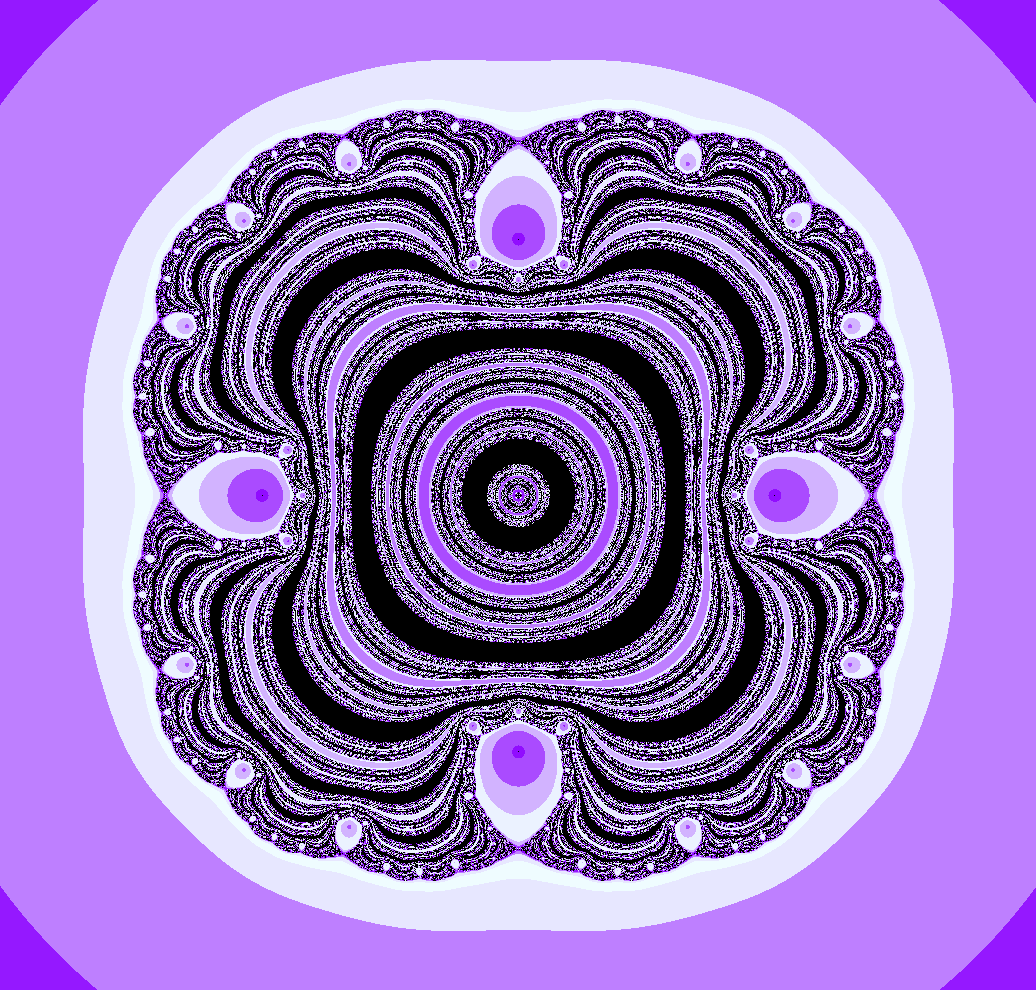


We remark that in [QYY15], Qiu, Yang and Yin have a similar result for rational maps with Cantor set of circles.
11. Equivalence of bounded escape and nested Julia sets
Recall that a hyperbolic component is said to admit bounded escape if there exists a sequence with markings so that
- (1)
is degenerating;
- (2)
For any periodic cycle of the topological model , the sequence of lengths is bounded.
Note that by definition, the hyperbolic component is, in particular, unbounded. In this section, we shall prove that a hyperbolic component has nested Julia sets if and only it admits bounded escape.
11.1. Nested Julia sets bounded escape
In this subsection, we shall prove the following using quasiconformal stretching.
Theorem 11.1.
Let be a hyperbolic component with nested Julia sets. Then it admits bounded escape.
Linear stretch of an annulus
Let , and let denote the round annulus . Given two round annuli and , we define a linear stretch between them as
where is the polar coordinate. We can extend the map continuously to unit disks by setting on . Note that is -quasiconformal, where .
Stretch of a hyperbolic rational map
Let be a hyperbolic rational map with nested Julia set, and let be critical gaps of . Then is a disk Fatou component. Note that may equal to . Let be a Riemann mapping. Since is hyperbolic, there exist so that contains no post-critical points for all . We define by replacing on , to
Note that for all sufficiently large , is -quasiregular.
Let , and . Since is pre-periodic, there are only finitely many components in . Define as identity if . Using the quasiregular map to pull back the standard complex structure on to on , and let be the corresponding quasiconformal map for . Then by Proposition 10.5, is quasiconformally conjugate to a rational map . We call a quasiconformal stretch of . Note that the modulus of is going to infinity, so the modulus of any critical annulus of is going to infinity.
By construction, each is quasiconformally conjugate to , so . Let be a gap of . Since is eventually mapped to a critical gap, the modulus of the corresponding annulus of is going to infinity. This implies that is degenerating. Indeed, otherwise, we can choose representatives and passing to a subsequence so that converges to a rational map of the same degree. Since the modulus of is going to infinity, at least one component of is shrinking to a point. So infinitely many pre-periodic points collapse to a single point, giving a contradiction.
We are now ready to prove Theorem 11.1.
Proof of Theorem 11.1.
Let be such a hyperbolic rational map. Let be a quasiconformal stretch of , with markings . Let be the corresponding map on the Shishikura tree. Let be a periodic point of of period . We consider two cases:
Case (1): is on the extremal Julia component . After passing to a second iterate, we may assume is fixed by and . Choose so that . Let , . Then is a polynomial like map.
Let and . Then is a polynomial like map. By construction of the quasiconformal stretch, we have . Since polynomial like map of degree with bounded below is compact up to affine conjugacy (see Theorem 5.8 in [McM94]), so converges compactly to of the same degree, so the multipliers of stay bounded.
Case(2): is on the non-extremal Julia component . Then by Lemma 10.1, is a Jordan curve and is buried. Let . Let be the norm of the derivative of at . Choose so that . Let and . Then and is a degree covering map.
Let and . By construction of the quasiconformal stretch, the moduli of the two annuli go to infinity. We normalize so that separates , and . Let be an annuli component of . Without loss of generality, we may assume that is in the unbounded component of . Then separates from . Since , (see Theorem 4.7 in [Ahl73]). Similarly, the other component of converges to . Hence, both and converges to . After passing to a subsequence, converges compactly on to a non-constant rational map. So the multiplier at is bounded in the subsequence.
Since the set of periodic cycles is countable, a diagonal argument allows us to pass to a subsequence and conclude admits bounded escape. ∎
11.2. Bounded escape nested Julia sets
We shall now prove the converse of Theorem 11.1. Let be a hyperbolic component that admits bounded escape. Let be the topological model for the actions on the Julia set for , and be the set of periodic cycles of . Then we have a sequence with markings which is degenerating, and for any , stay bounded. Recall that in §9, we have constructed a limiting dynamics
with the rescalings . The markings provide a marking on the end of the tree (see §9), so each periodic cycle represents a cycle of periodic ends for on .
The proof consists of two steps. We first classify the limiting dynamics that can appear. We then use the limiting dynamics to deduce the topological properties on the Julia set.
Classification of limiting map
Recall a periodic end is repelling if . Suppose has a cycle of repelling periodic ends, then by Theorem 1.2, it is represented by with , which is a contradiction. Hence, has no repelling periodic ends. We shall first classify those limiting dynamics with no repelling periodic ends.
Lemma 11.2.
Let , and . Let associated to , and such that
- (1)
;
- (2)
;
- (3)
does not intersect the critical tree nor contain .
Then has a repelling fixed end.
Proof.
Since does not intersect the critical tree, is an isometric bijection from to its image . Since does not intersect , .
Let be the preimage of in . Then , and . Hence, we can define inductively by taking the preimage of in . The union of the geodesic segments is an end which is fixed by . It is repelling as . ∎
The following lemma follows from our Theorem 7.3 and Theorem 10.83 in [BR10] (see also Proposition 9.3 in [RL05] and Lemma 6.2 in [RL03]).
Lemma 11.3.
Assume the limiting map has no repelling periodic ends. Then it has a fixed point of local degree .
Proposition 11.4.
Assume the limiting map has no repelling periodic ends. Let be a fixed point of multiplicity (which exists by Lemma 11.3). Then the set
is contained in a geodesic segment.
Proof.
By Theorem 4.2, there is no totally invariant point. Hence, the preimage of contains more than point. Note it suffices to show is contained in a line. Indeed, if we prove this, and escapes to one end, then replace by its second iterate if necessary, we get a repelling fixed end which is a contradiction.
We will now argue by contradiction to prove is contained in a line. Suppose not. Then there are two points which are eventually mapped to , and the convex hull of forms a ‘tripod’. Replacing by its iterate if necessary, we may assume that
Let be the tangent vector at associated to . There are two cases to consider:
Case : The preimage of under in is infinite. Then we can construct a ‘fan’ as follows (see Figure 11.1). Using Lemma 8.5, we construct inductively so that sends homeomorphically to . Let denote the tangent vector at associated to . Let be the tangent vectors at which is mapped to (there might be many such vectors, if that’s the case, we just choose one).
Inductively, we let be vector at which is mapped to . Note that the components are all disjoint. Since the critical tree for is a finite tree, there is a , such that for all and all , the component does not intersect the critical locus. Since is mapped to , is an isometric bijection from to its image by Lemma 8.3. Since the critical tree intersects (as is not injective on ), . Now by Lemma 11.2, we conclude that there is a repelling periodic end of period , which is a contradiction.

Case : The preimage of under in is finite. We remark that the idea is similar to the previous case, but the notations and indices become more complicated. By Theorem 8.1, replacing by its second iterate if necessary, we may assume is totally invariant under . Hence is (locally) expanding in the direction by Theorem 8.1. Let be the branched point of the tripod . Using Lemma 8.5, we choose so that maps homeomorphically to . We also choose so that maps and homeomorphically to and respectively.
We claim that at least one of and branches off in . Indeed, since is (locally) expanding in the direction , , so at least one of and must branch off (note that it may even happen before ). We assume branches off .
We denote , as the branched point of . Note that . We construct a generalized ‘fan’ using Lemma 8.5 as follows (see Figure 11.2).
First, by inductively taking preimages of , we construct so that sends homeomorphically to . Since is (locally) expanding in the direction and , and and .
We construct inductively so that sends homeomorphically to . Let denote the tangent vector at associated to . We define so that maps homeomorphically to . Let be a tangent vector at which is mapped .
Since the critical tree is finite, for large , the component does not intersect the critical locus. Thus is eventually an isometry between and , so there exists so that the length of is at least for all . Since , for sufficiently large , we can construct so that maps homeomorphically to . Inductively, for sufficiently large , we define so that is mapped homeomorphically to . We may assume that . Let be a tangent vector at which is mapped .
The argument is now similar to Case . Note that the components are disjoint. Since the critical tree for is a finite tree, there is a , such that for all and all , the component does not intersect the critical locus. Since is mapped to , is an isometry from to its image . Since the critical tree intersect , and , so . Now by Lemma 11.2, we conclude that there exists a repelling periodic end of period , which is a contradiction.

∎
Let be the smallest geodesic segment containing . Then sends the boundary to the boundary . As otherwise, we can find a point in with preimage outside of , which is a contradiction.
Let be the closure of a component of . Then maps homeomorphically to . Indeed, if the map is not injective, then there is a point with tangent vectors at associated to and respectively so that
But is surjective by Theorem 8.1, so there is a tangent vector which is mapped to the tangent vector at associated to either or . This means that intersects non-trivially with , which is a contradiction. The map is surjective by a similar argument: if is not surjective and let be the image. Note that is a subinterval of , so intersects non-trivially. By Theorem 8.1 and Lemma 8.5, the preimage of is not contained in , which is a contradiction.
We also note that has constant derivative on . Indeed, if not, then we can find a point with tangent vectors at associated to and respectively so that the local degrees at and are different. Then applying Theorem 8.1, one of has a preimage in other than . Then there is a point of in by Lemma 8.5, which is a contradiction.
By looking at the local degrees at the preimages of the point , we conclude the sum of the derivatives on different components equals .
To summarize, we have the following proposition, which describes the limiting dynamics with no repelling periodic ends.
Proposition 11.5.
Assume the limiting map has no repelling periodic ends. Let be a fixed point with multiplicity and . Let be the smallest geodesic segment that contains . Then there exist such that
- (1)
is a linear isometry with derivative and and the sign alternating;
- (2)
.
An immediate corollary of the above proposition is the following:
Corollary 11.6.
Let which is mapped into . Then contains no critical ends for all at not associated to or .
Proof.
Assume , so the norm of the derivative of at is . We first note that the local degree of at is . Otherwise, by counting critical points of , we conclude that the degree of is . Let and correspond to . Then by Theorem 8.1, there exists so that . By Lemma 8.5, there exists mapped to . This is a contradiction as is backward invariant.
Suppose contains a critical ends. Since the local degree of at is , Proposition 9.41 in [BR10] gives that . Again, this is a contradiction as is backward invariant. ∎
Remark 11.7.
We remark that we did not use the fact that comes from the same hyperbolic component yet. In our communication with Favre, a similar classification also appears in an unpublished manuscript by Favre and Rivera-Letelier. We would refer to [FRL10] where many such examples are studied.
From limiting map to nested Julia sets
We start with the following lemma. The proof uses standard expansion and pullback argument. For completeness, we sketch the proof and refer the readers to §5 in [PT00] for a more general setup.
Lemma 11.8.
Let be two annuli with , and let be a degree covering with . Then the non-escaping set is a Jordan curve.
Proof.
Let , and be two annuli component of so that is in the bounded component of . By Schwarz lemma, with respect to the hyperbolic metric on and in the domain and the codomain, the inclusion map is a contraction, and the covering map is an isometry. Thus, the map is expanding with respect to hyperbolic metric on . Since has compact closure in , expands a definite factor on .
Let be the component of so that is bounded by . By expansion, there exists a constant so that and (see Lemma 2 in §5 of [PT00]), and similarly for . Thus, has exactly two components , and .
Let be smooth simple closed curves that generate the fundamental group of , with parameterization . Inductively, let be the lift of . Choose a homotopy between and . By lifting this homotopy inductively, we construct parameterizations (see Lemma 0 in §5 of [PT00]). By expansion, converges uniformly to continuous maps (see Lemma 1 in §5 of [PT00]). Since is squeezed between , the image . In particular, is locally connected. By Lemma 5.1 in [PT00], is a Jordan curve. ∎
Let with markings that gives the bounded escape. Let be the limiting map. Let be the geodesic segment as in Proposition 11.5, and be a fixed point in . Then there exists an open set with boundary points and which is mapped to for some integer . By Corollary 11.6, contains no critical ends.
Let be sequences of annuli approximating as in Lemma 8.4. Then is a degree covering -almost surely. Since , by Lemma 8.2, -almost surely.
Let be in the -big set so that the above holds. Define the non-escaping set of by
Then is a Jordan curve by Lemma 11.8.
Since all comes from a single hyperbolic component, we will abuse notations and regard as in the topological model of the Julia set. The realization of in will be denoted by .
Let and .
Lemma 11.9.
is a nested set of circles.
Proof.
Let and so that and are disjoint from . Let and be domains approximating and respectively. Choose and .
We will now argue by induction: we assume that is a nested set of circles. Let . If with , then there exists and integer so that maps to . We may choose small enough so that . By Corollary 11.6, contains no critical ends. Let and be sequences approximating and as in Lemma 8.4. Then
is a degree covering -almost surely. Since , by Lemma 8.2 -almost surely. Since separates and , by Lemma 8.2, separates -almost surely. Similarly, any circle in separates -almost surely.
Let be in the -big set that satisfies the above properties. Let be the component of in . Then is still a nested set of circles, so is a nested set of circles. We can now add more -th preimages of into in a similar way. Therefore, by induction, is a nested set of circles. ∎
From the construction above, we also have
Proposition 11.10.
The natural ordering on the nested set is compatible with the linear ordering on , and the map sending a component of to the associated point in is a semi-conjugacy.
We are now ready to prove:
Theorem 11.11.
Let be a hyperbolic component. If is degenerating with markings such that
has no repelling periodic ends, then has nested Julia sets.
Proof.
Let . Abusing the notation, we assume the topological model of the action on the Julia set is given by .
First, we will show that the Julia set is disconnected. To show this, we will show , where is defined as in Proposition 11.5. Replacing by its second iterates and switch the role of and if necessary, we may assume is fixed by .
Let with , , and . We define to be the annulus bounded by and , then
is again an annulus. Let and be the -th in the linear ordering on of the preimages of and , and and respectively. Let be the annulus bounded by and , and
For each , since for sufficiently large , . Thus and the inclusion map is an isomorphism on fundamental groups. Since is a semi-conjugacy by Proposition 11.10, is mapped to as a degree covering, so . If , then by the equality case of the Grötzch inequality (see Theorem B.5 in [McM94]), and shares a Jordan curve boundary. Since , has a critical point on this boundary, which is a contradiction as this boundary is in the Julia set, and is hyperbolic.
Since , the non-escaping set is a Cantor set. Since , is not dense in , so is not connected.
Now we will prove every component separates two points. Let be close to , and . Let be bounded by containing the Julia component associated with . Then is a polynomial like map. Since the backward orbits of under the polynomial like restriction are all Jordan curves, the non-escaping set of is connected.
Thus, the extremal Julia component associated with is the Julia set associated to this polynomial like restriction. Since is hyperbolic, there exists a Fatou component of whose boundary is contained in . Similarly, we can find a Fatou component of whose boundary is contained in .
Let be two points. Then any Jordan curve in separates . Since , every component of separates . ∎
Remark 11.12.
If we have a degenerating sequence of flexible Lattès maps of degree , the limiting map also provides an example with no repelling periodic ends. In this case, we have and each (so ). Furthermore, the nested set of circle is dense in giving .
Now Theorem 1.5 is a straight forward consequence of the above results:
We also have the following theorem, which gives quantitative control on how periodic cycles escaping to infinity if is not nested.
Theorem 11.13.
Let be a hyperbolic component which does not have nested Julia sets, and let be a degenerating sequence with markings . Then there exists some with .
Open questions
We conclude our discussion on the length spectrum with the following open questions:
Question 11.14.
Let be a hyperbolic component admitting bounded escape. Do all degenerating sequences in this hyperbolic component have bounded multipliers?
Let be the modulus of the annulus bounded by the two extremal Julia components. If are bounded from below, then a similar argument as in the proof of Theorem 11.1 can be used to show that the lengths of a periodic cycle stay bounded. Therefore, to get an unbounded length spectrum, has to tend to . Conversely, if is degenerating and has bounded length spectrum, the proof of Theorem 11.11 implies that tends to . Therefore, the above is equivalent to the following:
Question 11.15.
Does there exist a positive lower bound for in ?
References
- [AM77] William Abikoff and Bernard Maskit. Geometric decompositions of Kleinian groups. Amer. J. Math., 99(4):687–697, 1977.
- [Ahl73] Lars Ahlfors. Conformal invariants: topics in geometric function theory. McGraw Hill, 1973.
- [Arf17] Matthieu Arfeux. Dynamics on trees of spheres. J. Lond. Math. Soc. (2), 95(1):177–202, 2017.
- [Bea91] Alan Beardon. Iteration of rational functions. Graduate texts in mathematics; 132. Springer-Verlag, New York, 1991.
- [Bes88] Mladen Bestvina. Degenerations of the hyperbolic space. Duke Math. J., 56(1):143–161, 1988.
- [Bes01] Mladen Bestvina. -trees in topology, geometry, and group theory. In R.J. Daverman and R.B. Sher, editors, Handbook of Geometric Topology, pages 55 – 91. North-Holland, Amsterdam, 2001.
- [BF14] Bodil Branner and Núria Fagella. Quasiconformal Surgery in Holomorphic Dynamics. Cambridge Studies in Advanced Mathematics. Cambridge University Press, 2014.
- [BR10] Matthew Baker and Robert S. Rumely. Potential Theory and Dynamics on the Berkovich Projective Line. Mathematical surveys and monographs. American Mathematical Soc., 2010.
- [Chi91] Ian Chiswell. Non-standard analysis and the morgan-shalen compactification. Q. J. Math., 42(1):257–270, 1991.
- [DE86] Adrien Douady and Clifford J. Earle. Conformally natural extension of homeomorphisms of the circle. Acta Math., 157:23–48, 1986.
- [DeM05] Laura DeMarco. Iteration at the boundary of the space of rational maps. Duke Math. J., 130(1):169–197, 2005.
- [DeM07] Laura DeMarco. The moduli space of quadratic rational maps. J. Amer. Math. Soc., 20(2):321–355, 2007.
- [dFM09] Tommaso de Fernex and Mircea Mustaţă. Limits of log canonical thresholds. Ann. Sci. Norm. Supér. (4), 42(3):491–515, 2009.
- [DM08] Laura DeMarco and Curtis McMullen. Trees and the dynamics of polynomials. Ann. Sci. Norm. Supér. (4), 41(3):337–383, 2008.
- [Eps00] Adam Epstein. Bounded hyperbolic components of quadratic rational maps. Ergodic Theory Dynam. Systems, 20(3):727–748, 2000.
- [Fab13a] Xander Faber. Topology and geometry of the Berkovich ramification locus for rational functions, I. Manuscripta Math., 142(3):439–474, 2013.
- [Fab13b] Xander Faber. Topology and geometry of the Berkovich ramification locus for rational functions, II. Math. Ann., 356(3):819–844, 2013.
- [FRL10] Charles Favre and Juan Rivera-Letelier. Théorie ergodique des fractions rationnelles sur un corps ultramétrique. Proc. Lond. Math. Soc. (3), 100(1):116–154, 2010.
- [Gro92] Misha Gromov. Asymptotic invariants of infinite groups. Geometric group theory. Volume 2. London Math. Society Lecture Notes, 182. Cambridge Univ. Press., 1992.
- [Hub06] John Hubbard. Teichmüller Theory and Applications to Geometry, Topology, and Dynamics: Teichmüller theory. Teichmüller Theory and Applications to Geometry, Topology, and Dynamics. Matrix Editions, 2006.
- [Jon15] Mattias Jonsson. Dynamics on Berkovich Spaces in Low Dimensions, pages 205–366. Springer International Publishing, Cham, 2015.
- [Kiw15] Jan Kiwi. Rescaling limits of complex rational maps. Duke Math. J., 164(7):1437–1470, 05 2015.
- [KL95] Michael Kapovich and Bernhard Leeb. On asymptotic cones and quasi-isometry classes of fundamental groups of 3-manifolds. Geom. Funct. Anal., 5(3):582–603, 1995.
- [LR75] A.H. Lightstone and Abraham Robinson. Nonarchimedean Fields and Asymptotic Expansions. North-Holland Mathematical Library. Elsevier, 1975.
- [Luo19] Yusheng Luo. Limits of rational maps, -trees and barycentric extension. Preprint. arXiv:1905.00915, 2019.
- [Luo20] Yusheng Luo. On hyperbolic rational maps with finitely connected Fatou sets. J. Lond. Math. Soc. (2) to apear, arXiv:2004.02797, 2020.
- [McM88] Curtis McMullen. Automorphisms of rational maps. In Holomorphic Functions and Moduli I, volume 10 of Mathematical Sciences Research Institute Publications, pages 31–60. Springer, 1988.
- [McM94] Curtis McMullen. Complex Dynamics and Renormalization (AM-135). Princeton University Press, 1994.
- [McM08] Curtis McMullen. Thermodynamics, dimension and the Weil-Petersson metric. Invent. Math., 173(2):365–425, 2008.
- [McM09a] Curtis McMullen. A compactification of the space of expanding maps on the circle. Geom. Funct. Anal., 18(6):2101–2119, 2009.
- [McM09b] Curtis McMullen. Ribbon -trees and holomorphic dynamics on the unit disk. J. Topol., 2(1):23–76, 2009.
- [McM10] Curtis McMullen. Dynamics on the unit disk : short geodesics and simple cycles. Comment. Math. Helv., 85(4): 723–749, 2010.
- [MS84] John Morgan and Peter Shalen. Valuations, trees, and degenerations of hyperbolic structures, I. Ann. of Math. (2), 120(3):401–476, 1984.
- [MS98] Curtis McMullen and Dennis Sullivan. Quasiconformal homeomorphisms and dynamics III. the Teichmüller space of a holomorphic dynamical system. Adv. Math., 135(2):351 – 395, 1998.
- [NP20] Hongming Nie and Kevin Pilgrim. Boundedness of hyperbolic components of newton maps. Israel J. Math., 238:831 – 869, 2020.
- [Ota96] Jean-Pierre Otal. Le théorème d’hyperbolisation pour les variétés fibrées de dimension 3. Asterisque, Société Mathématique de France, (235), 1996.
- [Pau88] Frédéric Paulin. Topologie de Gromov équivariante, structures hyperboliques et arbres réels. Invent. Math., 94(1):53–80, 1988.
- [Pet11] Carsten Petersen. Conformally natural extensions revisited. arXiv:1102.1470, 2011.
- [PT00] Kevin Pilgrim and Lei Tan. Rational maps with disconnected Julia set. Asterisque, Société Mathématique de France, 261:349–384, 01 2000.
- [QYY15] Weiyuan Qiu, Fei Yang, and Yongcheng Yin. Rational maps whose julia sets are cantor circles. Ergodic Theory Dynam. Systems, 35(2):499–529, 2015.
- [RL03] Juan Rivera-Letelier. Espace hyperbolique -adique et dynamique des fonctions rationnelles. Compos. Math., 138(2):199–231, 2003.
- [RL05] Juan Rivera-Letelier. Points périodiques des fonctions rationnelles dans l’espace hyperbolique -adique. Comment. Math. Helv., 80(3):593–629, 2005.
- [Roe03] John Roe. Lectures on Coarse Geometry. American Mathematical Society, Providence, 2003.
- [Shi87] Mitsuhiro Shishikura. On the quasiconformal surgery of rational functions. Ann. Sci. Éc. Norm. Supér. (4), 20(1):1–29, 1987.
- [Shi89] Mitshuhiro Shishikura. Trees associated with the configuration of Herman rings. Ergodic Theory Dynam. Systems, 9(3):543–560, 1989.
- [Sti93] James Stimson. Degree two rational maps with a periodic critical point. PhD thesis, University of Liverpool, 1993.