Local to global property in free groups

I would like to thank Michael Chapman for introducing me to these local to global questions for free groups, and asking me to give a lecture about them in a Stallings’ graphs seminar that he and Noam Kolodner organized at the Hebrew university. Here is hoping that next time I will not have to read a paper that was never meant to be read.

The research leading to these results has received funding from the European Research Council under the European Union Seventh Framework Programme (FP/2007-2013) / ERC Grant Agreement n. 335989.

Now that we have our new topological notation, let us sketch the main idea of the reduction step, where as example we consider the equation $x^{m}=g$.

1. (1)

   Fix some $g\in G=F_{k}$ and assume that $g$ is an $m$-power in every finite quotient of $F_{k}$ or equivalently there is some $h\in\hat{G}$ such that $h^{m}=g$. Letting $H=\overline{\left\langle h\right\rangle}\leq\hat{G}$ , assume first that there is some $g\in H_{0}\leq F_{k}$ finitely generated such that $\widehat{H}_{0}\cong\overline{H_{0}}=H$, namely

   The group $H_{0}$ is free as a subgroup of a free group, and therefore $H_{0}\cong F_{k^{\prime}}$ for some $k^{\prime}$ (it is also finitely generated). On the other hand, its completion $\hat{H}_{0}\cong\overline{\left\langle h\right\rangle}$ is generated topologically by one element $h$, so we must have that $k^{\prime}=1$. In other words, this reduces the problem to $H_{0}\cong\mathbb{Z}$ and $\hat{H}_{0}\cong\hat{\mathbb{Z}}$ where we already know the local to global principle for $m$-powers (or additively - multiples of $m$).

2. (2)

   However, the conditions above are not true in general. In order to fix this problem, let $H_{0}$ be a finitely generated subgroup such that $g\in H_{0}$ and $\overline{H_{0}}\leq H$. Suppose that we can find a surjective continuous map $\pi:H\to\overline{H_{0}}$ which fixes $\overline{H_{0}}$, so we have the diagram

   where $\pi\circ\iota=Id_{\overline{N}}$. In this case we get that (1) $\overline{H_{0}}$ will be generated topologically by $\pi\left(h\right)$ and $(2)$ we have that $\pi\left(h\right)^{m}=\pi\left(h^{m}\right)=\pi\left(g\right)=g$ because $g\in\overline{H_{0}}$ is fixed by $\pi$. We can now use the trick from above for $\left\langle g\right\rangle\leq H_{0}\leq\overline{H_{0}}\leq\hat{G}$.
   As we shall see, this result will be more general, and not only for the $m$-power equations. The interpretation of this result will be that if $w\in F_{n}$ is any word (e.g. $w=x^{m},\left[x,y\right]$ etc.) and we want to prove the local to global property for it, namely that a solution to $w\left(\hat{g}_{1},...,\hat{g}_{n}\right)=g$ in $\hat{G}$ implies a solution in $G$, it is enough to prove this claim under the further assumption that $\hat{g}_{1},...,\hat{g}_{n}$ generate $\hat{F}_{k}$, so in particular $k\leq n$. In the finite quotients language, it means that the solution $\hat{g}_{1}K,...,\hat{g}_{n}K$ generate the group $\nicefrac{{G}}{{K}}$ for every $K\underset{f.i.}{\trianglelefteq}G$.

3. (3)

   The two main problems in (2) above are to somehow define a homomorphism from $H$ to $\overline{H_{0}}$ and moreover it needs to fix $\overline{H_{0}}$. However, there is one such situation where this is very easy. Suppose that $H_{0}$ is a free factor $H_{0}\leq_{*}N$ of some group $N\leq F_{k}$, namely we can write $N=H_{0}*H_{1}$ for some subgroup $H_{1}$. Then there is a natural projection $\pi:N\to H_{0}$ which fixes $H_{0}$. We can then extend it to their completion $\overline{\pi}:\overline{N}\to\overline{H}_{0}$, and if $H\leq\overline{N}$ then the restriction of $\overline{\pi}$ to $H$ will do the job

The main result of the next section will be to show that we can actually choose such $H_{0}$ and $N$ “wisely” so that $H_{0}\leq_{*}N$ and $H\leq\overline{N}$.

The Stallings graphs will be our main tool to understand subgroups of the free group, and to say when one subgroup is a free factor of another. Before we define them, consider the following example of a labeled graph (defined below).

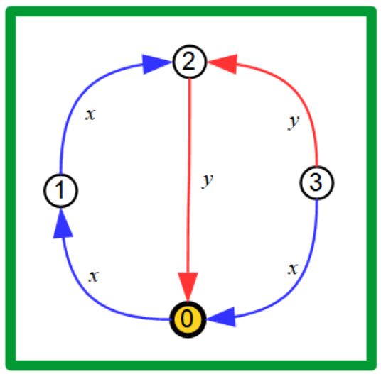
This graph has two “main” cycles corresponding to $x^{2}y$ on the left and $x^{-1}y^{2}$ on the right, and every other cycle can be constructed using these two cycles (up to homotopy, i.e. modulo backtracking). Furthermore, the labeling allows us to think of these cycles as elements in $F_{2}=\left\langle x,y\right\rangle$, so that the fundamental group of the graph could be considered as the subgroup generated by $x^{2}y$ and $x^{-1}y^{2}$. With this example in mind, we now give the proper definitions to make this argument more precise.

One of the most basic results in algebraic topology is that the fundamental group of a graph is always a free group. Let us recall some of the details.

It is not hard to show that any cycle in a connected graph can be written as a concatenation of cycles in $C\left(T\right)$ and their inverses as elements in the fundamental group $\pi_{1}\left(\Gamma\right)$ (namely, we are allowed to remove backtracking). More over, it has a unique such presentation which leads to the following:

In particular, the corollary above implies that the fundamental group of the bouquet graph with a single vertex and $n$ self loops is the free group $F_{n}$. We can label the edges by their corresponding basis elements $x_{1},...,x_{n}$ of $F_{n}$. Since it is important in which direction we travel across the edge, we will think of each edge as two directed edges labeled by $x_{i}$ and $x_{i}^{-1}$ depending on the image in the fundamental group. For simplicity, we will keep only the edges with the $x_{i}$ labeling, understanding that we can also travel in the opposite direction via an $x_{i}^{-1}$ labeled edge.

It is well known that a fundamental group of a covering space correspond to a subgroup of the original space. Using the generalization of the labeling above we can produce covering using the combinatorics of labeled graphs.

For the rest of this section we fix a basis $x_{1},...,x_{n}$ of the free group $F_{n}$.

We denote by $\Gamma_{F_{n}}$ the bouquet graph with the $x_{1},...,x_{n}$ labeling. Note that another way to define a labeling on a graph $\Gamma$ is a morphism of directed graphs $\varphi:\Gamma\to\Gamma_{F_{n}}$ where the labeling of an edge $e\in E\left(\Gamma\right)$ is defined to be the labeling of $\varphi\left(e\right)$. In this way a labeled graph morphism is just a map which defines a commuting diagram

This labeling map $\varphi:\Gamma\to\Gamma_{F_{n}}$ induces a homomorphism $\hat{\varphi}:\pi_{1}\left(\Gamma,v\right)\to\pi_{1}\left(\Gamma_{F_{n}}\right)=F_{n}$. Since every path in $\Gamma$ is sent to a cycle in $\Gamma_{F_{n}}$, we can extend this map to general paths in $\Gamma$.

In general, for a labeled graph $\varphi:\Gamma\to\Gamma_{F_{n}}$ the function $\hat{\varphi}$ is not injective. However, in the Stallings graphs case, defined below, it is.

In the Stallings graph case, it is an exercise to show that $\hat{\varphi}$ is injective, and we may consider $\pi_{1}\left(\Gamma,v\right)$ as a subgroup of $F_{n}$. Moreover, we can use 3.1 to find a basis for $\pi_{1}\left(\Gamma,v\right)$ as a subgroup of $F_{n}$.

One way to construct Stallings graphs is by starting with a standard labeled graph, and then taking a suitable quotient. We will use this construction to build such graphs for subgroups of $F_{n}$.

It is easy to check that if $\left(\Gamma,v\right)$ is a labeled graph, then the quotient graph $\left(\nicefrac{{\Gamma}}{{\sim}},\left[v\right]\right)$, where $\left[v\right]$ is the image of $v$, is a Stallings graph. We will usually also remove any edges and vertices which are not part of a simple cycle, since these do not change the fundamental group.

With our new language of Stallings graphs, we can now prove how a simple condition of injectivity implies that one subgroup is a free factor of another subgroup.

If $H\leq N\leq F_{n}$ then we can construct the two Stallings graphs $\Gamma_{H},\Gamma_{N}$ and then there is a natural labeled morphism $\Gamma_{H}\to\Gamma_{N}$. If this morphism is injective, then by the claim above we know that $H\leq_{*}N$ is a free factor of $N$. However, the injectiveness of this map depends also on our initial choice of basis for $F_{n}$, and in general $H$ can be a free factor of $N$ even when the corresponding graph morphism is not injective. The next result uses the Stallings graphs to show how to naturally find two subgroups where the Stallings graphs are injective, and therefore one is a free factor of the other. As we shall see later, this type of result is exactly what we need in our reduction in 3.1.

Let $g\in F_{k}$ and $m\in\mathbb{Z}$. Our profinite notation shows that $x^{m}=g$ has the local to global property if a solution over $\hat{F}_{k}$ implies a solution over $F_{k}$. This is a very special type of equation which can be written as $w=g$, where the left side contains only parameters and the right side contain only $g$. In this section we provide the details for the ideas in 3.1 for this type of equations and then the specialization for $x^{m}=g$ will lead to the proof of 1.6.

For the rest of this section, we will have two free groups. The first will be denoted by $F_{n}$ and the free variables will be from it, while the second $G=F_{k}$ will be the group in which we try to prove the local global principle.

Finally, we can use this reduction to prove that $w=x^{m}$ has the local to global property for free groups.

References

- [1] Tullio Ceccherini-Silberstein and Michel Coornaert. Cellular Automata and Groups. Springer Monographs in Mathematics. Springer-Verlag, Berlin Heidelberg, 2010.
- [2] Anatole Khelif. Finite approximation and commutators in free groups. Journal of Algebra, 281(2):407–412, November 2004.
- [3] Luis Ribes and Pavel Zalesskii. Profinite Groups. Springer Science & Business Media, March 2010. Google-Books-ID: u8GWrhdhA2QC.
- [4] John G. Thompson. Power Maps and Completions of Free Groups and of the Modular Group. Journal of Algebra, 191(1):252–264, May 1997.
- [5] John S Wilson. Profinite groups. Clarendon Press ; Oxford University Press, Oxford; New York, 1998. OCLC: 40658188.