-Corrected Heisenberg Limit
Abstract
We consider the precision with which the parameter , appearing in the unitary map acting on some type of probe system, can be estimated when there is a finite amount of prior information about . We show that, if acts times in total, then, asymptotically in , there is a tight lower bound , where , are the extreme eigenvalues of the generator . This is greater by a factor of than the conventional Heisenberg limit, derived from the properties of the quantum Fisher information. That is, the conventional bound is never saturable. Our result makes no assumptions on the measurement protocol, and is relevant not only in the noiseless case but also if noise can be eliminated using quantum error correction techniques.
Introduction and statement of result. The Heisenberg limit (HL) is the central concept for the whole field of quantum metrology research as it epitomizes the potential of optimal quantum metrology protocols to surpass standard schemes that are restricted by the so-called standard quantum limit (SQL) Giovannetti et al. 2006; Paris 2009; Giovannetti et al. 2011; Toth and Apellaniz 2014; Demkowicz-Dobrzanski et al. 2015; Schnabel 2017; Degen et al. 2017; Pezzè et al. 2018; Pirandola et al. 2018. For the canonical example of interferometry to measure a stationary optical phase, these two limits are expressed in terms of the number of photon passes through the unknown phase. The HL for the estimation precision is conventionally given as , while the SQL corresponds simply to the shot-noise precision limit. This scaling improvement can be achieved using entangled photon states Mitchell et al. 2004, or multiple passes Higgins et al. 2007, or a combination of both Daryanoosh et al. 2018. In all such cases the essential feature is that phase is being accumulated coherently over the uses of the probe system, unlike in standard schemes where each probe (photon) interferes only with itself and the whole procedure is repeated times gathering statistics that leads to improvement of precision.
In a generalized phase estimation scenario, evolution of a probe system is given by a unitary , where is an arbitrary Hermitian generator of the transformation. In what follows, we allow the spectrum of to be arbitrary, apart from being bounded from above and from below by and respectively. Hence, the parameter is not necessarily restricted to the interval. Analysis of the problem using the concept of the quantum Fisher information (QFI) and the quantum Cramér-Rao (CR) bound leads to the following SQL and HL respectively Giovannetti et al. 2006:
| (1) |
where is the number of repetitions of the experiment, is the number of applications of the unitary in a single repetition of the experiment, The SQL corresponds to the situation when independent interrogations of the probe system are performed in a single experiment, while the HL takes into account the most general interrogation scheme involving uses of . That may include coherent sequential probes, entangled probes, as well as the most general adaptive schemes. Interestingly, in such noiseless unitary parameter estimation scenarios there is no advantage to using adaptive strategies, as the simplest sequential scenario where the phase is being coherently imprinted on a single probe times already leads to the above stated HL. The fundamental advantage that entanglement and adaptiveness offer emerges in the CR bound only when noise is present Demkowicz-Dobrzański and Maccone 2014.
Importantly, by the nature of the CR bound, the above bounds are guaranteed to be saturable only in the limit of many repetitions, . On the other hand, when considering repetitions, the total number of unitary operations involved is . The most general way of using those resources is to allow entanglement between all, in which case the HL in terms of total resources is rather than scaling Hayashi et al. 2018. That corresponds to using in Eq. (1), in which case saturability cannot be guaranteed.
In many papers, the saturability discussion focuses on the existence of a measurement for which the Fisher information of the corresponding probabilistic model coincides with the QFI Braunstein and Caves 1994. Such a measurement indeed always exists, defined by the eigenbasis of the symmetric logarithmic derivative operator. However, even with such a measurement chosen, the existence of an estimator that saturates the CR bound is guaranteed in single-shot scenarios only if the value of the parameter is known exactly beforehand or in the case of a narrow class of probabilistic models called the exponential family Fend 1959.
In this Letter, we prove that the asymptotically tight HL includes an additional factor:
| (2) |
More formally, . The condition under which we prove this bound is that any prior information is limited. For example, one could require that there be a prior probability distribution for which is bandlimited or piecewise constant, or that the measurement work over some finite region in -space. Most importantly, the prior information must be independent of . That is, if you are given more resources , you cannot change the task by demanding a sharper prior distribution, or further restricting the region of validity of your measurement. This requirement is necessary to make the HL a meaningful concept; otherwise, the prior information is comparable to the information from the measurement itself. The -corrected limit we derive comes precisely from eliminating the influence of any (implicit or explicit) prior.
Equation (2) was conjectured in Jarzyna and Demkowicz-Dobrzański 2015, but the argument was indirect and restricted to the standard parallel qubit phase estimation scheme with Gaussian prior, and the potential impact of adaptiveness was not analyzed. Since the HL is the key benchmark against which any theoretically conceived or experimentally implemented quantum-enhanced strategy is compared, it is essential to phrase it as an actual attainable limit, unlike its most commonly encountered form, Eq. (1), which is not achievable even in principle. Our result is also timely, given the recent revival of interest in quantum error correction inspired metrological protocols which allow estimation with HL scaling even in the presence of some particular noise types Sekatski et al. 2017; Demkowicz-Dobrzański et al. 2017; Layden and Cappellaro 2018; Zhou et al. 2018. The proper phrasing of the HL is vital not only for idealized noiseless metrological scenarios but also in the case of more realistic noisy ones.

In our analysis, we use the Bayesian approach to estimation, also called random parameter estimation, in which a probability distribution is given that describes the prior knowledge of . In the case where no prior is known, also called non-random parameter estimation Kay 1993, the usual approach is to require that the measurement be locally unbiased. Local unbiasedness allows one to derive the traditional (not -corrected) form of the HL given in Eq. (1), and ensures that, typically, the estimator approximately achieves the claimed mean-square error (MSE) over some finite range of . However, it does not ensure that this finite region is independent of . Since the true value of cannot be known before making the measurement, a useful measurement must work over a fixed region, even as increases. Thus it is appropriate to consider the average of the MSE over some fixed region. Mathematically, that is equivalent to Bayesian estimation with a flat prior over the region, and so there is no loss of generality in using a Bayesian approach.
It is necessary to exclude pathological priors, which could lead to arbitrarily high precision. We do this by requiring the prior to be well approximated by a finite bandwidth function (i.e. a function whose Fourier transform has bounded support). As we will show, this is not a very restrictive condition; in particular, the results will be valid for any prior that may be approximated by a weighted sum of flat priors with nonzero fixed width : , where is the Heaviside step function. That includes the case where the MSE is averaged over a finite region, used to address cases with an unknown prior. Provided the above regularity condition holds, the actual form of the prior becomes irrelevant for sufficiently large . The intuition behind this result is that, in the limit of , the amount of data that can potentially be gathered on the parameter is unlimited and hence overwhelms any impact of the prior on the final precision.
Proof of result. Consider the most general adaptive estimation scheme, Fig. 1 (i). Here is the input state of a probe system potentially entangled with an arbitrary number of ancillary systems, and are control unitary operations applied between interrogation steps where the unknown parameter is imprinted on the probe system. The final state at the output is measured using a generalized measurement described by a positive operator valued measure , where the index represents the estimated value of the parameter upon attaining that outcome from the measurement. The minimal expected (in the Bayesian sense) mean-square error in the estimation thus reads:
| (3) |
Let us analyze the structure of the state as it evolves through the subsequent gates and control operations. Each gate multiplies components of the state, as decomposed in the eigenbasis, by one of the factors ( represents some eigenvalue of ), while control operations perform a basis change. In the end, after coherent interrogations of the unknown parameter , the final state will have the following structure:
| (4) |
where are complex amplitudes and are some normalized vectors which in general will not be orthogonal. The key feature of this state is that it has bandwidth bounded by , as will any inner products with this state.
Now let be the prior with a finite bandwidth , so that its Fourier transform is supported on an interval of length . It is known that in all single-generator unitary estimation problems with quadratic cost one may restrict the class of measurements to rank-one projective ones Helstrom 1976; Macieszczak et al. 2014. Let us assume for a moment a fixed input state and a measurement basis with a corresponding estimator . The corresponding cost reads
| (5) |
Now, from Boas Jr et al. 1945, it is possible to find a function with bandwidth such that . Let us define functions (which have bandwidths bounded by ) and . We have:
| (6) |
The product of two bandlimited functions gives a function which is bandlimited by the sum of the bandwidths, so has a bandwidth at most . We can then write
| (7) |
with
| (8) | ||||
| (9) |
The task of minimizing for a given is equivalent to that of minimisation for , because the optimal can be shifted by any amount without altering the bandwidth. We may also set (this just sets the normalization of the function ). After applying the Fourier transform, the minimization problem reads
| (10) |
subject to the constraints
| (11) |
Here the boundary conditions are due to the restricted bandwidth of . This is equivalent to the problem of finding the minimum energy eigenstate in an infinite potential well with width . The solution for that achieves the minimum is a sine curve (see Fig. 1(ii)), which gives , and hence
| (12) |
That is, provided the prior has a limit on its bandwidth, the Heisenberg limit (2) holds in the limit of large —i.e. when the prior correction becomes negligible.
Now we need only prove that any reasonable prior may be well approximated by a finite bandwidth function. To first show this informally, let us introduce a family of non-negative normalized finite bandwidth functions
| (13) |
where is the bandwidth, is a parameter that controls the size of the tails and is a normalization factor that for large. This is proportional to the fourth power of the Fourier transform of the Kaiser window Kaiser and Schafer 1980 of width , so has bandwidth . The function has width , beyond which the tails are exponentially suppressed in , like . Thus for large it approximates the Dirac delta function and therefore any reasonable prior may be approximated by its convolution with , i.e. , for which the bandwidth is also .
In particular, we may show that, for any prior of the form , the following bound holds:
| (14) |
where . This gives
| (15) |
which after taking the square root of both sides proves Eq. (2).
Here we just sketch the reasoning leading to the above claim, whereas the complete proof with all the technical details is presented in the Supplementary Materials SM. First, we lower bound the minimal cost in the case that the prior is actually a single rectangular prior of width at . Note that this will also be a legitimate lower bound for the original problem where the prior is a weighted sum of such rectangular priors, as the optimal strategy for this original problem cannot perform better than the optimal strategy when we additionally know to which interval the value of our parameter is restricted. Then, we approximate the rectangular prior via a distribution obtained by convolving a slightly narrower rectangular distribution (narrower by ) with the function, as defined in Eq. (13)—see Fig. 1(iii). By setting and appropriately, we can guarantee that all the deviations of the resulting cost due to modifications of the prior from the strictly rectangular one introduce no more than ( indicates that logarithmic multipliers are ignored) relative correction compared with the cost corresponding to the distribution. Finally, the cost corresponding to the distribution can be bounded using Eq. (12) thanks to the finite bandwidth property of .
In the case of non-random parameter estimation Kay 1993, we average the MSE over a -interval of size . This is equivalent to using a flat prior of width , so our bound holds in this case also, and this is true regardless of whether or not the estimators are unbiased. The conventional scenario of unbiased estimators with no average does typically mean that the measurement works well for within some finite region. However, the size of that region may depend on . That is, as increases the region of validity for an unbiased measurement may shrink with . This is exactly the case for the NOON states Kok et al. 2002 that maximize the CR bound, saturating the conventional HL in Eq. (1). For these states the probability distributions obtained are periodic in with period , and the interval in where the CR-saturating measurement is useful shrinks exactly as fast in as the CR bound itself.
To reiterate, to make the HL a meaningful concept, the bound should not rely on using more and more prior information as increases, because that would mean that the prior information can be comparable to the information from the measurement itself. To derive a HL that describes the information obtained from the measurement, one must do as we have done, and take a prior that is independent of , or require a region of validity that is independent of . Then the information about in the limit comes only from the measurement on the state. Eliminating the influence of prior information is what gives our additional factor of .
Discussion. Having derived the bound let us now discuss its saturability. It is known that in the case of a standard phase estimation problem with applied in parallel to qubits the optimal Bayesian strategy for flat prior distribution () in the limit of large yields Berry and Wiseman 2000. Note also, that the optimal strategy involves application of the so called covariant measurements Holevo 1982, and a covariant measurement strategy will yield the same average cost irrespective of the form of prior. Hence the limit is saturable in the case of an arbitrary prior as well. In the case of an estimation problem with a general generator , we can say that provided the prior is supported on an interval smaller than we can directly adapt the reasoning from the standard qubit phase estimation scheme by considering our elementary system as a qubit with only two accessible states being the eigenstates of corresponding to and . This way we obtain . However, if our prior is broader, then clearly using this strategy we will not be able to discriminate between phases that differ by a multiple of as they effectively would lead to the same output state. In order to discriminate between these phases we would need to use additional eigenstates of corresponding to intermediate eigenvalues (provided they are available). If we use levels corresponding to eigenvalues that differ by , we may discriminate between all phases which differ by less than . Note that for our purposes, the minimal level splitting may be effectively obtained as a difference between sums of certain finite number of energy levels , and a result may be smaller than the minimal level splitting in the itself. Since the discrimination error drops exponentially with the number of resources used, we may sacrifice sublinear (in ) uses of the channel for the purpose of this additional discrimination task and this will not affect the final scaling.
The phase estimation problem may be viewed as a special case of a more general frequency estimation problem, where the probe system is allowed to be interrogated for the total interrogation time and the goal is to estimate a frequency-like parameter entering into the Hamiltonian of the system as , with being some Hermitian operator. The total interrogation time may be split into a number of shorter evolution steps each lasting time . Assuming the prior distribution satisfies the regularity assumption and can be written as a sum of rectangular priors of some finite width we may repeat the whole reasoning as presented above by formally identifying , , and arrive at
| (16) |
This is the valid asymptotically saturable bound for the most general frequency estimation adaptive strategies in the limit of long total interrogation time . In particular in all the cases where, despite presence of noise, the Heisenberg scaling is being recovered via e.g. application of quantum error-correction inspired techniques Kessler et al. 2014; Dür et al. 2014; Arrad et al. 2014; Demkowicz-Dobrzański et al. 2017; Sekatski et al. 2017; Zhou et al. 2018; Layden and Cappellaro 2018, it is the above bound that should be used as a operationally meaningful figure of merit of such protocols and not the standard QFI based one.
Finally, since Eq. (14) is not tight for finite , the form of the exact achievable bound in nonasymptotic case is an interesting open question for future research.
Acknowledgements.
We thank Michael Hall, Marcin Jarzyna, Paweł Kasprzak, Jan Kolodynski and Yuval Sanders for fruitful discussions. WG and RDD acknowledge support from the National Science Center (Poland) grant No. 2016/22/E/ST2/00559. DWB is funded by Australian Research Council Discovery Projects DP160102426 and DP190102633. HMW is funded by the Australian Research Council Centre of Excellence Program CE170100012.References
- Giovannetti et al. (2006) V. Giovannetti, S. Lloyd, and L. Maccone, Phys. Rev. Lett. 96, 010401 (2006).
- Paris (2009) M. G. A. Paris, Int. J. Quantum Inf. 07, 125 (2009).
- Giovannetti et al. (2011) V. Giovannetti, S. Lloyd, and L. Maccone, Nat. Photonics 5, 222 (2011).
- Toth and Apellaniz (2014) G. Toth and I. Apellaniz, J. Phys. A: Math. Theor. 47, 424006 (2014).
- Demkowicz-Dobrzanski et al. (2015) R. Demkowicz-Dobrzanski, M. Jarzyna, and J. Kołodyński, in Prog. Optics, Vol. 60, edited by E. Wolf (Elsevier, 2015) pp. 345–435.
- Schnabel (2017) R. Schnabel, Phys. Rep. 684, 1 (2017).
- Degen et al. (2017) C. L. Degen, F. Reinhard, and P. Cappellaro, Rev. Mod. Phys. 89, 035002 (2017).
- Pezzè et al. (2018) L. Pezzè, A. Smerzi, M. K. Oberthaler, R. Schmied, and P. Treutlein, Rev. Mod. Phys. 90, 035005 (2018).
- Pirandola et al. (2018) S. Pirandola, B. R. Bardhan, T. Gehring, C. Weedbrook, and S. Lloyd, Nat. Photonics 12, 724 (2018).
- Mitchell et al. (2004) M. W. Mitchell, J. S. Lundeen, and A. M. Steinberg, Nature 429, 161 (2004).
- Higgins et al. (2007) B. L. Higgins, D. W. Berry, S. D. Bartlett, H. M. Wiseman, and G. J. Pryde, Nature 450, 393 (2007).
- Daryanoosh et al. (2018) S. Daryanoosh, S. Slussarenko, D. W. Berry, H. M. Wiseman, and G. J. Pryde, Nature Communications 9, 4606 (2018).
- Demkowicz-Dobrzański and Maccone (2014) R. Demkowicz-Dobrzański and L. Maccone, Phys. Rev. Lett. 113, 250801 (2014).
- Hayashi et al. (2018) M. Hayashi, S. Vinjanampathy, and L. C. Kwek, Journal of Physics B: Atomic, Molecular and Optical Physics 52, 015503 (2018).
- Braunstein and Caves (1994) S. L. Braunstein and C. M. Caves, Phys. Rev. Lett. 72, 3439 (1994).
- Fend (1959) A. V. Fend, The Annals of Mathematical Statistics 30, 381 (1959).
- Jarzyna and Demkowicz-Dobrzański (2015) M. Jarzyna and R. Demkowicz-Dobrzański, New J. Phys. 17, 013010 (2015).
- Sekatski et al. (2017) P. Sekatski, M. Skotiniotis, J. Kołodyński, and W. Dür, Quantum 1, 27 (2017).
- Demkowicz-Dobrzański et al. (2017) R. Demkowicz-Dobrzański, J. Czajkowski, and P. Sekatski, Phys. Rev. X 7, 041009 (2017).
- Layden and Cappellaro (2018) D. Layden and P. Cappellaro, npj Quantum Inf. 4, 30 (2018).
- Zhou et al. (2018) S. Zhou, M. Zhang, J. Preskill, and L. Jiang, Nat. Commun. 9, 78 (2018).
- Helstrom (1976) C. W. Helstrom, Quantum detection and estimation theory (Academic press, 1976).
- Macieszczak et al. (2014) K. Macieszczak, M. Fraas, and R. Demkowicz-Dobrzański, New Journal of Physics 16, 113002 (2014).
- Boas Jr et al. (1945) R. Boas Jr, M. Kac, et al., Duke Mathematical Journal 12, 189 (1945).
- Kaiser and Schafer (1980) J. Kaiser and R. Schafer, IEEE Transactions on Acoustics, Speech, and Signal Processing 28, 105 (1980).
- (26) See Supplemental Material for detailed proofs.
- Kay (1993) S. M. Kay, Fundamentals of Statistical Signal Processing: Estimation Theory, edited by S. E. Alan V. Oppenheim (Prentice Hall, 1993).
- Kok et al. (2002) P. Kok, H. Lee, and J. P. Dowling, Phys. Rev. A 65, 052104 (2002).
- Berry and Wiseman (2000) D. W. Berry and H. M. Wiseman, Phys. Rev. Lett. 85, 5098 (2000).
- Holevo (1982) A. S. Holevo, Probabilistic and Statistical Aspects of Quantum Theory (North Holland, Amsterdam, 1982).
- Kessler et al. (2014) E. M. Kessler, I. Lovchinsky, A. O. Sushkov, and M. D. Lukin, Phys. Rev. Lett. 112, 150802 (2014).
- Dür et al. (2014) W. Dür, M. Skotiniotis, F. Frowis, and B. Kraus, Phys. Rev. Lett. 112, 080801 (2014).
- Arrad et al. (2014) G. Arrad, Y. Vinkler, D. Aharonov, and A. Retzker, Phys. Rev. Lett. 112, 150801 (2014).
Supplemental Material
Appendix A Lower bounding the Bayesian cost using rectangular priors
Given the minimal Bayesian cost as in Eq. (3) with a prior that is a weighted sum of rectangular priors
| (17) |
we can obtain the following lower bound:
| (18) |
In the first line we have used Eq. (3) from the main text and substituted the expression for . In the second line, the inequality is due to the fact that we can optimize the estimation strategy for each rectangular prior separately, and we have also limited the integral over to the region where is nonzero. In the third line, we have used the fact that the cost corresponding to shifted rectangular priors should be the same. That is, given the optimal strategy for a given rectangular prior, we can obtain an equally good estimation strategy for a prior shifted by amount , by first counter-rotating the input state by a phase , performing the same measurement as before and adding the appropriate shift into the finally estimated value. The factor of arises because the normalization of means that the sum over must be . This implies that the minimal Bayesian cost for the prior which is a weighted sum of rectangular priors of width cannot be smaller than the minimal Bayesian cost for a problem with a prior which is a single normalized rectangular prior of width .
Note that this same approach works for any prior that is obtained from a convolution
| (19) |
Following the same reasoning as above,
| (20) |
That is, if the prior probability distribution is obtained by convolving with , then the mean-square error can be lower bounded by that using as the prior. For the case of rectangular priors above, would be a rectangle function of width , and would be a series of delta functions with height spaced apart by .
Appendix B Normalization for finite-bandwidth function
Here we discuss some features of the family of non-negative normalized finite bandwidth functions:
| (21) |
where is a normalization constant depending on . As mentioned in the main text, this is the fourth power of the Fourier transform of the Kaiser window function of bandwidth , and hence has a bandwidth .
First note that the function significantly changes its behavior at . For the sinh is exponentially large in , which must be compensated for by the normalization factor being exponentially small. In contrast, for the function becomes the fourth power of a sinc, so decreases as . Moreover, the exponentially small normalization factor means that these tails are exponentially small in . Now we would like to estimate the value of the normalization factor for large values of . When integrating the function within the interval we can obtain the following approximation
| (22) | ||||
| (23) | ||||
| (24) |
In (22) we note that the hyperbolic sine is dominated by , so we can replace the by 1 in the denominator. We also omitted the terms and in as they have much smaller impact than . We have kept because it enables the simplification in the next line. In (23) we have approximated the zeroth-order modified Bessel function of the first kind by . Now we can bound the impact of sinc tails as
| (25) |
We see that this quantity, when compared with (24), is negligible for large and therefore .
By expanding in a Taylor series about and using the asymptotic expansion of modified Bessel functions, it is also possible to obtain corrections as
| (26) |
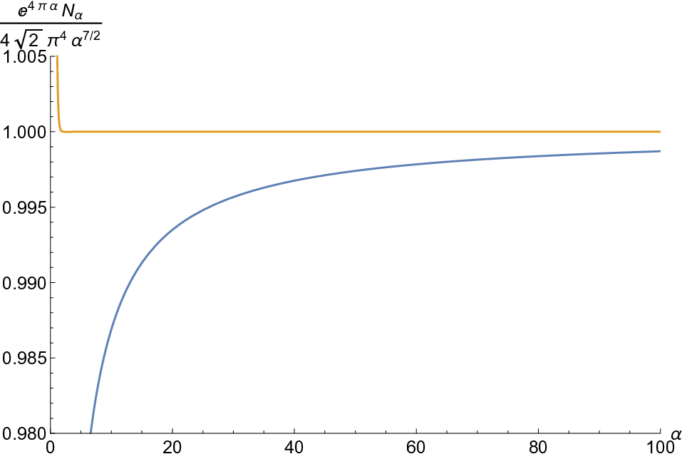
Note that all correction terms are negative. In practice we find that , as well as it being an accurate approximation, as shown in Figure 2.
Appendix C Proof of the bound for the estimation cost in case of a rectangular prior in the limit of large
Now we will demonstrate how the result valid for a finite-bandwidth prior may be utilized to get a bound for the rectangular prior of size , which will be denoted as . The most intuitive way to approximate the prior by a finite bandwidth function is to convolve it with . However, the distribution constructed in such a way would differ from the initial one by some non-negligible parts that stick outside of the original rectangular distribution. To avoid this problem, we consider a slightly narrowed rectangular prior of width and only then perform the convolution
| (27) |
This procedure guarantees that only the sinc-like tails will stick outside the range of the initial rectangular distribution after the convolution is performed.
Note that
| (28) |
For we have , so
| (29) |
Let represent the optimal measurement/estimator strategy for the rectangular prior . Then must be for as the optimal strategy never estimates a value of the parameter outside of the support of the prior. Therefore we obtain
| (30) |
If we extend the limits of integration over on the right side of the inequality to , we may lower bound the resulting quantity by the minimal conditional cost corresponding to the finite bandwidth prior , i.e. . Therefore, we have
| (31) |
where corresponds to the tails of the distribution
| (32) |
To bound we use the following chain of inequalities (we start with the right tail):
| (33) | ||||
| (34) | ||||
| (35) | ||||
| (36) | ||||
| (37) |
In (33) we have replaced all the estimated values with the extreme value ; in (34) we have substituted the exact formula for (27); in (35) we have shifted the variable , and in (36) we have modified the integration limits, while keeping the actual integration region unchanged.
Now, from the fact that and using inequalities and , we may bound the above integral by
| (38) |
For notational clarity, let us introduce a small dimensionless parameter . The above expression now takes the form:
| (39) |
Analogous reasoning holds for the left tail . Therefore, we have:
| (40) |
The integral in (39) may be calculated exactly and yields (assuming that ):
| (41) |
which may be bounded by (see Figure 3).

After substituting into (31) and using we have
| (42) |
which now may be optimized over (with the restriction ). In particular, defining , if we take , then
| (43) |
If we then choose
| (44) |
then the last term is higher order, and we get
| (45) |
using to indicate that logarithmic factors are omitted. In fact, it is possible to give this inequality without the term as
| (46) |
This inequality may be obtained numerically, by comparing the right-hand side (RHS) of Eq. (42) to that of Eq. (46) as a function of , as shown in Figure 4. This inequality is equivalent to Eq. (14) of the main text. The RHS of Eq. (46) is only positive for , so the inequality is only useful in that regime. That also ensures that our assumption holds. It is found that the RHS of Eq. (42) is larger than that of Eq. (46), so Eq. (42) implies Eq. (46).
