Cross-layer Design for Mission-Critical IoT in Mobile Edge Computing Systems
Abstract
In this work, we propose a cross-layer framework for optimizing user association, packet offloading rates, and bandwidth allocation for Mission-Critical Internet-of-Things (MC-IoT) services with short packets in Mobile Edge Computing (MEC) systems, where enhanced Mobile BroadBand (eMBB) services with long packets are considered as background services. To reduce communication delay, the 5th generation new radio is adopted in radio access networks. To avoid long queueing delay for short packets from MC-IoT, Processor-Sharing (PS) servers are deployed at MEC systems, where the service rate of the server is equally allocated to all the packets in the buffer. We derive the distribution of latency experienced by short packets in closed-form, and minimize the overall packet loss probability subject to the end-to-end delay requirement. To solve the non-convex optimization problem, we propose an algorithm that converges to a near optimal solution when the throughput of eMBB services is much higher than MC-IoT services, and extend it into more general scenarios. Furthermore, we derive the optimal solutions in two asymptotic cases: communication or computing is the bottleneck of reliability. Simulation and numerical results validate our analysis and show that the PS server outperforms first-come-first-serve servers.
Index Terms:
Mission-critical internet-of-things, mobile edge computing, 5G new radio, processor-sharing server, cross-layer optimizationI Introduction
Mission-Critical Internet-of-Things (MC-IoT) will be widely deployed in future wireless networks for remote health monitoring, haptic interaction, and factory automation [2, 3]. Achieving ultra-reliable and low-latency communications (URLLC) (e.g., packet loss probability and ms End-to-End (E2E) delay) for MC-IoT has been considered as one of the major goals in 5th Generation (5G) cellular networks [4]. Most existing technologies mainly focus on one of the seven layers of the open systems interconnection model, and cannot guarantee the E2E delay [5]. To satisfy the requirements of MC-IoT, we need to re-design the physical-layer resource management, the link-layer scheduling policy, and the network-layer user association from a cross-layer perspective.
One of the major differences between MC-IoT and enhanced Mobile BroadBand (eMBB) services lies in the sizes of packets. With high data rate, the packet size in eMBB services is relatively large, e.g., thousands of bytes in each packet. However, the packets generated by MC-IoT are very small, e.g., or bytes in each packet [6]. To achieve low latency for short packet transmissions, a short frame structure is adopted in 5G New Radio (NR) [7]. When transmitting a short packet in a short frame, the blocklength of channel codes is very limited. As a result, the decoding error probability cannot be ignored when analyzing reliability [8].
On the other hand, the computing ability at each MC-IoT device is limited. To reduce processing delay, MC-IoT devices will offload some of the packets to the Mobile Edge Computing (MEC) systems for processing [9, 10]. Considering that MC-IoT services will co-exist with eMBB services, a short packet arriving at the MEC after long packets has to wait in a queue if the packets are processed with a First-Come-First-Serve (FCFS) order. To avoid long queueing delay, other scheduling orders at MEC systems should be considered.
Furthermore, the reliability and delay not only depend on the resource management and scheduling order but also depend on the traffic load. Considering that the radio resources and computing capacity at each Access Point (AP) are limited, the user association and offloading policy should be optimized to balance traffic loads. The problems for optimizing user association and offloading policy are NP-hard in general [11]. Low-complexity solutions to the NP-hard problems are in urgent need for MC-IoT since complicated searching algorithms will lead to long computation delay [12].
I-A Related Works
To transmit short packets with low latency, the blocklength of channel codes is short. In the short blocklength regime, Shannon’s capacity is not applicable since it cannot characterize the decoding error probability [8]. Recently, the maximal achievable rate with given decoding error probability in the short blocklength regime was obtained in multi-antenna quasi-static channel [13]. How to design transmission schemes and resource allocation in the short blocklength regime has been studied in existing literature [14, 15, 16, 17, 18, 19, 20]. The throughput achieved in cognitive radio channels and relay systems was studied in [14] and [15, 16], respectively. The studies in [17] optimized the scheduling of short packets to maximize energy efficiency. The authors of [18] optimized packet losses caused by decoding errors, queueing delay violation, and packet dropping over deep fading channel subject to the ultra-high reliability. Considering that the feedback of Channel State Information (CSI) leads to extra delay, the studies in [19] jointly optimized Uplink (UL) and Downlink (DL) resource configurations without CSI at the transmitters. More recently, how to optimize resource allocation among multiple users with different packet arrival processes was studied in [20].
Scheduling policies in computing systems have significant impacts on the Quality-of-Service (QoS) of MC-IoT. A near-optimal policy to minimize the average latency of short packet is the Shortest Remaining Processing Time (SRPT) first scheduler. Such a scheduler is hard to implement in practice since the remaining processing time is not available at the server, and it requires too many priority levels[21]. To reduce the latency of short packets without introducing priority levels, the Processor-Sharing (PS) server is a possible solution, where the total service rate is equally allocated to all the packets in the server[22]. Although the distribution of latency was derived in the large delay regime in the PS server [23], the latency experienced by short packets remains unclear. To derive the delay bound violation probability of URLLC services, martingales-based analysis, effective capacity, and network calculus were used in [24], [15], and [25], respectively. But all the results were obtained in the FCFS servers. Note that it is very challenging to derive the closed-form expression of the distribution of delay, how to formulate the constraints on delay and reliability of MC-IoT is still unclear.
Promising network architectures for MC-IoT were studied in [26, 27, 28, 29, 30]. A comprehensive overview on MC-IoT of industrial scenarios was carried out in [26], where the issues related to architecture design were discussed, such as extensibility, scalability, and modularity. To reduce the routing delay, an adaptive transmission architecture with software-defined networks and edge computing was proposed in [27]. Considering that energy consumption of IoT devices is an important issue, an energy-aware real-time routing scheme was proposed in [27] to reduce energy consumption and E2E delay in large-scale IoT networks. More recently, a fog computing architecture was proposed for 5G tactile IoT [29], where the quality-of-experience-aware model was formulated. By combining stochastic geometry and queueing theory, different QoS requirements were analyzed in ultra-dense networks [30]. The studies in [26, 27, 28, 29, 30] shed light upon network architecture designs for MC-IoT, but decoding errors in the physical-layer were not considered.
Computing offloading has been exhaustively studied in various MEC systems, such as wireless powered MEC [31], ultra-dense IoT networks [32, 33], and fiber-wireless networks [34, 35]. Although these works did not consider MC-IoT, they developed useful methodologies for optimizing computing offloading in MEC systems. How to improve the QoS in MEC systems by optimizing task offloading has been addressed in [36, 37, 38, 39]. In [36], the average delay was minimized by optimizing task offloading/scheduling in MEC systems. Considering that the average delay is not suitable for URLLC services, the authors of [37] optimized task offloading and resource allocation under the constraint on a queue length violation probability. The offloading schemes for URLLC in MEC systems were optimized in [38], where a weighted sum of E2E delay and the offloading failure probability was minimized in a single-user scenario. How to analyze latency in large-scale MEC networks was studied in [39], where the average communication and computing latencies were derived.
Most of the existing studies on resource management in MEC systems only analyzed UL transmission and processing delay, and assumed DL transmission can be finished with high transmit power at the APs [36, 37, 39, 38]. Besides, they did not take the decoding errors in the short blocklength regime into account, which is crucial for MC-IoT. Although the block error probability was considered in the optimization problem in [38], the radio resource management was not optimized and the packet losses due to the delay bound violation were not considered.
I-B Our Contributions
To the best of the authors’ knowledge, there is no resource allocation scheme or offloading scheme that can achieve the target E2E delay and overall packet loss probability for MC-IoT in MEC systems. Moreover, how to design scheduling policy and whether the FCFS server is suitable for MC-IoT were not addressed. In order to achieve ultra-high reliability and ultra-low E2E delay for MC-IoT in MEC systems, the following three issues will be addressed in this work: 1) How to design scheduling and queueing policies in MEC servers and local servers to achieve ultra-high reliability and ultra-low E2E delay for short packets? 2) How to characterize the statistical QoS of short packets when there are both short and long packets in MEC systems? 3) How to improve the fundamental tradeoff between delay and reliability by optimizing user association, packets offloading, and bandwidth allocation in MEC systems? Our major contributions are summarized as follows,
- •
We establish a framework for minimizing overall packet loss probability subject to E2E delay requirement in MEC systems, where processing delay and UL and DL transmission delays are taken into account. PS servers are equipped at MEC systems, where the total service rate is equally allocated to all the packets in each server, and every packet receives service at all times. As such, short packets can bypass long packets and achieve low latency.
- •
We derive a closed-form approximation of the Complementary Cumulative Distribution Function (CCDF) of the latency experienced by short packets in the PS server. The approximation is accurate when the number of Central Processing Unit (CPU) cycles needed to process a long packet is much larger than that needed to process a short packet.
- •
We optimize the user association scheme, packet offloading rates, and bandwidth allocation for short packets in MEC systems. We propose an algorithm to solve a mixed integer problem and analyze the convergence and the complexity of it. Our analysis shows that the difference between the obtained solution and the global optimal solution only results from searching numbers of subcarriers in a continuous domain.
Furthermore, our simulation results validate the accuracy of the closed-form approximation. Numerical results indicate that when increasing the number of antennas at the AP with a fixed processing capacity, communication is the bottleneck of the reliability when the number of antennas is small, and computing is the bottleneck when the number of antennas is large. Only in a very small region (e.g., from to antennas), the packet loss probability in communications is comparable to the processing delay violation probability. This implies our algorithm converges to a near optimal solution in most of the cases.
The rest of the paper is organized as follows. Section II describes the system model. Section III analyzes delay and reliability. Section IV studies how to optimize the association scheme, packet offloading rates and bandwidth allocation. Section V extends the algorithm into more general scenarios. Section VI provides simulation and numerical results. Section VII concludes the paper.
II System Model
II-A The MEC System
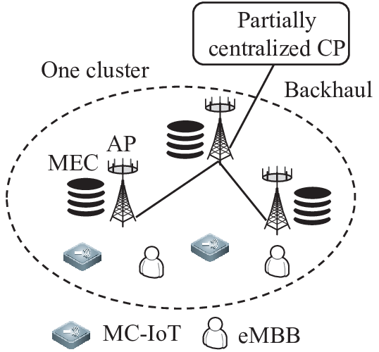
As illustrated in Fig. 1, we consider a MEC system with single-antenna devices and multi-antenna APs, where the data collected by each MC-IoT device and the computation intensive tasks generated by eMBB services can be offloaded to one of the APs for processing. To provide better services in radio access networks and to avoid high backhaul overhead, the partially centralized Control Plane (CP) in [12] is considered. The whole network is decomposed into multiple clusters, each of which includes closely located APs and one CP that optimizes user association scheme, packet offloading rates, and bandwidth allocation for devices in the cluster. To achieve ultra-low latency and ultra-high reliability, strong co-channel interference should be avoided. To this end, orthogonal channels are allocated to different devices in each cluster, and the frequency reuse factor is less than one such that adjacent clusters use different bandwidth. In this work, we focus on one cluster of APs, and our solution is applicable for low mobility scenarios like factory automation and VR/AR applications. For high mobility scenarios, where devices travel across clusters frequently, how to reserve resources in different clusters deserves further study.
II-B Traffic Models
In vehicle networks and factory automation, there are two kinds of packets, i.e., periodic packets with deterministic arrivals and sporadic packets that are driven by some random events [40, 41]. Since analyzing the delay and the reliability of random packet arrival processes is more challenging than deterministic arrivals, we focus on sporadic packets in this work. The experiment in [42] indicates that the packet arrival processes of MC-IoT are very bursty, i.e., there is a high traffic state and a low traffic state. For each of the traffic states, the arrival process can be modeled as a Bernoulli process. According to 5G NR, time is discretized into slots with duration . In each slot, a device either has a packet to transmit or stays silent. We assume the traffic state is obtained with the traffic state classification methods in [42]. When a device switches between the high and low traffic states, we only need to change the average arrival rate in our analysis. The aggregation of multiple independent Bernoulli processes at a MEC server can be accurately approximated by a Poisson process [43].
II-B1 Short packets
The data collected by each MC-IoT device is contained in short packets for transmission and processing. A packet with the following three features is considered as “short”,
- •
The number of bits in the packet is small. According to [6], the packet size in MC-IoT services is around or bytes. In contrast, the packets in eMBB services may include hundreds or thousands of bytes, such as video streaming.
- •
The blocklength of channel codes of the packet is short. For example, if quadrature phase-shift keying is used in modulation, the number of symbols required by a packet with bytes ( bits) is , which is the blocklength of the packet. To achieve low-latency, the blocklength of channel codes is short in MC-IoT [44].
- •
The number of CPU cycles required to process the packet is small. The number of CPU cycles required to process the packet depends on the number of bits in the packet and the processing algorithms. Since a packet in MC-IoT services only contains a few bits, the number of required CPU cycles is small.
Let be the number of CPU cycles required to process a short packet. The service rate of the local server at the th device and that of the th MEC server are denoted as and , respectively.
II-B2 Long packets
There are some devices requesting eMBB services in each cluster. The tasks generated by the eMBB services are packetized into long packets. How to optimize resource allocation and computing offloading for eMBB services has been studied in the existing literature, such as [45, 46, 47]. In our work, we focus on MC-IoT services, where eMBB services are considered as background services.
The sum of average packet arrival rates of eMBB services at the th AP is denoted as (packets/slot). The number of CPU cycles required to process a long packet is denoted as , which is a random variable with mean value . In this work, we do not specify the distribution of . The only assumption on is that , which is reasonable since the packet size of eMBB services is much larger than that of MC-IoT services and the algorithm for processing long packets (e.g., high definition pictures) is more complex than that for processing short packets (e.g., the location and velocity of a device). For example, may follow the Pareto distribution with a heavy tail [22], i.e.,
| (1) |
where , , and is the minimum of . As shown in [22] and the references therein, Pareto distributions have been observed in different application scenarios, such as the service time of UNIX jobs.
II-C User Association and Packet Offloading
II-C1 User association
Each device can associate with one of the APs. We leverage indicators , to represent the user association scheme,
The association scheme of the th device is denoted as .
II-C2 Packet offloading
When a short packet is generated by the th device, the device either processes the packet with the local server or uploads the packet to an AP. The average packet rate from the th device to the th MEC server is denoted as (packets/slot), where and . means that the packets are processed at the local server. If , then , where is the average packet arrival rate of the th device. If for all , then .
II-D Queueing Models and Scheduling Policies

As shown in Fig. 2(a), to guarantee the QoS requirements of different devices, packets from different devices are waiting in different queues at a MEC server, and are served according to the FCFS order. In the th MEC server, the service rate allocated to the th device is denoted as . Once the computing resource is allocated to one device, it cannot be shared with the other devices. Such a scheduling scheme is widely used, but is not optimal in terms of minimizing the delay.
The second server in Fig. 2(b) is referred to as a statistical multiplexing FCFS server [22]. Due to statistical multiplexing gain, the average delay in the second server is much shorter than the first server when . Furthermore, as proved in [19], if the sizes of all the packets are identical, to achieve the same delay bound and delay bound violation probability, the required service rate in the statistical multiplexing server is less than the sum of the service rates in the individual server. However, when the distribution of the number of CPU cycles required to process the packets has a heavy-tail, some short packets arriving at the MEC server after a long packet need to wait for a long time. As a result, the delay requirement of MC-IoT services can hardly be satisfied.
The key to low latency is letting short packets bypass queued long packets. One possible solution is the PS server. As shown in Fig. 2(c), every packet in the server receives service at all times. When there are packets in the th MEC server, each packet is processed at rate .
Remark 1.
In practice, a server can be implemented in a time-sharing way, i.e., the service time in each slot is equally allocated to all the packets in the server. In this way, the processing delay of packets in the server is the same as that in the ideal PS server [22]. It’s worth noting that there are some other possible scheduling policies if the server is aware of the diverse QoS requirements of different packets. In this work, we do not assume the computing system is aware of the types of packets in the communication systems. We will study more sophisticated scheduling policies for different types of packets in our future work.

We consider the scheduling policies at MEC servers and local servers in Fig. 3, where PS servers are deployed at APs and FCFS servers are deployed at devices. To avoid queueing delay, the UL and DL transmission durations of a short packet equal to one slot.11 1 Since the packet arrival rate of each device is less than one packet per slot, there is no queue before UL and DL transmissions. On the other hand, if the required CPU cycles to process different packets are identical, which is the case in the local server of each device, the FCFS server outperforms the PS server [22]. Therefore, FCFS servers are equipped at MC-IoT devices.
III Analysis of Delay and Reliability
In this section, we study how to characterize E2E delay and overall packet loss probability. We first derive the CCDF of the processing delay of short packets in the PS server. Then, we show how to characterize the transmission delay and decoding error probability of short packets.
III-A Processing Delay and Delay Violation Probability
A short packet can be processed either at the device or at the AP. The packet arrival process at the local server of the th device is a Bernoulli process with average arrival rate . Denote the service time of a packet at the th local server as . With the constant service rate at each local server, the queueing model is a Geo/D/1/FCFS model, where “Geo” means that the inter-arrival time between packets is geometric distributed, and “D” represents deterministic service processes. The CCDF of queueing delay in Geo/D/1/FCFS model has been obtained in [48]. If , then
| (4) |
If , the expression of can be found in [48]. Due to the low-latency requirement, we are interested in the case .
Each AP may serve multiple devices. The aggregation of multiple Bernoulli processes can be modeled as a Poisson process [39]. Thus, the MEC server can be characterized by an M/G/1/PS model, where “M” means the packet arrival process is Poisson process and “G” means that the number of CPU cycles required to process the packets can follow any distributions. To derive a closed-form CCDF of the processing delay of short packets in the M/G/1/PS model, we introduce an accurate approximation. Since the short packets are much smaller than the long packets, i.e., , the processing delay of a short packet is much shorter than a long packet. As a result, the number of long packets in the server is nearly constant from the arrival to the departure of a short packet. When a short packet arrives at the server, the number of packets in the server is denoted as . Considering that the value of does not change significantly during the short service time of a short packet, then the service rate allocated to the short packet can be approximated by if . In this case, the processing delay of the short packet is approximated by
| (5) |
According to [22], the distribution of can be expressed as follows,
| (6) |
which is the distribution of the number of packets in the M/G/1/PS model. The workload of the server is
| (7) |
From (5) and (6), we can further obtain that
where . Based on the above expression, the CCDF of the processing delay of short packets in the PS server can be derived as follows,
| (8) |
The approximation in (8) is accurate when . We will validate the accuracy of the approximation via simulation.
The processing delay of short packets in the th MEC server can be characterized by a delay bound and a delay bound violation probability, and . From the CCDF in (8), the relationship between and can be expressed as follows,
| (9) |
III-B Transmission Delay and Decoding Error Probability
If a packet is processed at the MEC server, the device first uploads the packet to the AP. After the MEC server finishes the processing, the result is sent back to the device. We introduce a superscript of parameters , where . If , is a parameter in UL transmissions. Otherwise, it is a parameter in DL transmissions. We consider Orthogonal Frequency Division Multiple Access (OFDMA) systems, which will be used to support MC-IoT services in 5G NR [7]. The total bandwidth is equally allocated to subcarriers, each with a bandwidth of . Denote the number of subcarriers allocated to the th device for UL and DL transmissions as , , respectively. Since the packet size is small, it is reasonable to assume that is smaller than the coherence bandwidth. As mentioned in the previous section, to avoid queueing delay before UL and DL transmissions, the transmission duration of each packet is one slot, which is smaller than channel coherence time. Thus, each packet is transmitted over a flat fading quasi-static channel. Considering that feedback from receivers to transmitters may cause large overhead and extra delay, CSI is not available at the transmitters. According to [13], the achievable rate in the short blocklength regime over quasi-static flat fading channel can be accurately approximated by
| (10) |
where is the large-scale channel gain from the th device to the th AP, is the UL or DL small-scale channel fading between the th device and the th AP, is the UL or DL transmit power of one antenna on each subcarrier, is the single-side noise spectral density, is the inverse of Q-function, is the decoding error probability, and .
Remark 2.
Due to the following two reasons, we only consider the flat fading channel, and do not consider frequency-selective channels. First, the maximal achievable rate over a frequency-selective channel in the short blocklength regime has not been derived in existing studies. Although the upper and lower bounds were obtained in [49], there is no closed-form expression. Second, as shown in [19], when the number of antennas is large (e.g., antennas), frequency diversity is not necessary for URLLC. Therefore, we focus on the multi-antenna flat fading channel.
Let be the number of bits in a short packet of the th device. When sending a packet of bits within one slot, the decoding error probability can be obtained from (10) by setting . According to the law of total probability, the packet loss probability due to decoding errors can be expressed as follows [13],
| (11) |
where the distribution of small-scale channel gain depends on the number of antennas at each AP, which is denoted as . To compute (11), we need to calculate the integral for a given distribution of . For Rayleigh fading, we can apply the closed-form result in [50].
III-C E2E Delay and Overall Packet Loss Probability
III-C1 Delay and Reliability at Local Servers
If a packet is processed at the device, then the E2E delay is equal to the sum of the service time and the queueing delay at the local server of the device. Given the E2E delay requirement , the delay violation probability at local servers, , can be obtained by substituting into (4). When ,
| (12) |
III-C2 Delay and Reliability at the MEC server
If a packet is processed at a MEC server, then the UL and DL transmission delays and the processing delay in the server should be considered. The E2E delay can be satisfied under the following constraint,
| (13) |
where two slots are occupied by the UL and DL transmissions.
Due to decoding errors and processing delay violation, the overall packet loss probability can be expressed as follows,
| (14) |
where the approximation is very accurate since , , and are extremely small in MC-IoT. Upon substituting (7) and (13) into (9), we can get the expression of , i.e.,
| (15) |
Remark 3.
The factors that lead to packet losses or errors depend on network architectures [51]. For the considered MEC system, reliability only includes queueing delay violations in computing systems and packet losses in radio access networks.
IV Cross-Layer Optimization
In this section, we study how to optimize the association scheme, packet offloading rates, and UL and DL bandwidth allocation to minimize the overall packet loss probability subject to the E2E delay requirement.
IV-A Problem Formulation
Note that the packet loss probabilities at the local server and the MEC can be different, the reliability is determined by the worse one. Thus, the packet loss probability of the th device is characterized by
| (16) |
The problem that minimizes the maximal packet loss probability experienced by the devices can be formulated as follows,
| (17) | ||||
| s.t. | (17a) | |||
| (17b) | ||||
| (17c) | ||||
| (17d) | ||||
| (17e) |
where , , is the maximum number of subcarriers that can be allocated to a device without exceeding the coherence bandwidth, and the expressions of , , and can be found in (11), (12), and (15), respectively. Constraint (17a) guarantees that a device can only associate with one AP. If , then all the packets are processed at the local server.
With constraint (17a), each device cannot be served by two or more APs. Constraint (17b) ensures that the packet offloading rate is zero if the th device is not served by the th AP. Constraint (17c) guarantees that the sum of the packet offloading rates at the APs and the packet arrival rate at the local server is equal to the total packet arrival rate of a device. The constraint on the maximal number of subcarriers of the system is given in (17d), where the UL and DL bandwidth allocated to each device does not exceed the coherence bandwidth. When constraint (17e) is satisfied, and are smaller than , and hence the local and MEC servers are stable. By minimizing the objective function, we can check whether constraint (17e) can be satisfied or not. If it cannot be satisfied, the problem is infeasible.
Since CSI is not available at the transmitters, the transmit power on each subcarrier is fixed. In UL transmission, the maximal transmit power of a device, , is equally allocated to subcarriers, . In DL transmission, the maximal transmit power of an AP, , is equally allocated to antennas. Considering that the number of subcarriers for DL transmission can be up to , to satisfy maximal transmit power constraint, the transmit power on each subcarrier is fixed as . Thus, we have .
Problem (17) is a mixed integer optimization problem, which is non-convex. In typical scenarios, the throughput of eMBB services is much higher than the throughput of MC-IoT services, and hence the number of CPU cycles required to process long packets are much larger than that required to process short packets. In the rest part of this section, we first consider the scenario that , and then extend our algorithm into more general scenarios.
IV-B Solution in the Typical Scenario
IV-B1 Simplified Optimization Problem
According to (17c), . Thus, we have
| (18) |
When , the equality in (18) holds, and in (15) is a constant that does not depend on packet offloading rates. Moreover, the packet loss probabilities due to decoding errors in UL and DL transmissions, and , do not change with packet offloading rates. Thus, the second term in does not depend on packet offloading rates. By setting , all the packets are offloaded to the MEC servers. Then, and
| (19) |
With (19), problem (17) can be simplified as follows,
| (20) | ||||
| s.t. |
IV-B2 Packet Loss Balance Algorithm
Denote the optimal solution and the minimal packet loss probability of problem (20) as and , respectively. In the following, we propose a binary search algorithm to find the optimal solution. The basic idea of the algorithm is to keep below a threshold , and search the minimal in the regime , where is an initial upper bound of the overall packet loss probability. We refer to the algorithm as the Packet Loss Balance (PLB) Algorithm.
For a given threshold of overall packet loss probability , we search for the optimal association scheme and subcarrier allocation that minimize the total number of subcarriers. If the minimum number of subcarriers exceeds , then . Otherwise, .
The problem that minimizes the total number of subcarriers can be expressed as follows,
| (21) | ||||
| s.t. | (21a) | |||
where constraint (17e) is removed since . The above problem can be decoupled into problems since the association schemes and bandwidth allocation of different devices are independent.
Given that the th device is served by the th MEC server, , the required number of subcarriers can be found from the following problem,22 2 By solving problem (22) with different , we can obtain the optimal user association scheme and related bandwidth allocation that minimize .
| (22) | ||||
| s.t. | (22a) | |||
To solve the inter programming problem, we first relax and as continuous variables, and find the optimal subcarrier allocation. Then, we discretize the number of subcarriers used in UL and DL transmissions. Note that only the discretization step will cause performance loss, which is minor as shown in [52].
Property 1.
The packet loss probabilities and in (11) are convex in .
Proof.
See proof in Appendix A. ∎
Further considering that in (15) does not change with , constraint (22a) is convex. Therefore, problem (22) is a convex problem, and can be solved by techniques such as the interior-point method [53]. The algorithm for solving problem (21) is provided in Table I, where is the minimum integer that is equal to or higher than .
Note that problem (21) could be infeasible if is too small. In this case, the minimal overall packet loss probability is higher than . Based on the algorithm in Table I, the PLB algorithm for solving problem (20) is shown in Table II.
IV-B3 Convergence of the PLB Algorithm
To prove that the PLB algorithm converges to the minimal packet loss probability of problem (20), we first prove the following proposition,
Proposition 1.
The minimal packet loss probability lies in the region , .
Proof.
See proof in Appendix B. ∎
According to Proposition 1, the minimal packet loss probability lies in the region . After steps of searching, the gap between and the output of the PLB algorithm, , is smaller than . In addition, with the binary search algorithm (i.e. from Line 1 to Line 11 in Table II), the range of decreases according to the following expression, . When is large enough, approaches to .
The above proof holds when the performance loss caused by the discretization step in Line 7 of Table I is negligible. Since the discretization step inevitably causes some performance loss, the related association scheme and bandwidth allocation are near optimal.
IV-B4 Complexity of the PLB Algorithm
With the PLB algorithm, we need to solve problem (21) around times. Problem (21) is decoupled into single-device problem in (22). With the algorithm in Table I, the convex optimization problem in (22) is solved times for devices with possible APs. The complexity of solving the convex optimization problem is denoted as , which is not high. Therefore, the complexity of the PLB algorithm is . Considering that a device will not associate with an AP that is very far from it, will not be very large. For example, a device can only be connected to one of the three or four APs with the highest large-scale channel gains. As a result, the complexity of the PLB algorithm increases linearly with the number of devices.
V Solution in General Scenarios
To solve problem (17), we extend the PLB algorithm into general scenarios without the assumption .
V-A Extended PLB Algorithm
Although problem (17) cannot be simplified as problem (20), we can still use the algorithm in Table II. The difference between the general scenarios and the scenario with the assumption lies in Line 3 of the algorithm, where problem (21) is obtained from (20). In general scenarios, given the threshold of overall packet loss probability, , the optimization problem that minimizes the total number of subcarriers can be expressed as follows,
| (23) | ||||
| s.t. | (23a) | |||
From the expression of in (15), we can see that increases with the packet offloading rate . Besides, the expressions of and in (11) show that the required number of subcarriers increases as decreases. Therefore, to satisfy constraint (23a), the number of subcarriers increases with the packet offloading rate . To minimize the total number of subcarriers, the first step is minimizing packet offloading rates.
Step 1: Optimize offloading rates. To minimize packet offloading rates, we find the maximal packets arrival rate at the local server, denoted as . Note that the delay violation probability at each local server should satisfy , by substituting the expression of in (12) into the constraint, can be obtained via binary search. If , all the packets are processed at the local server, , , and . Otherwise, the packet offloading rate of the th device is . As such, the constraint on the packet offloading rate in (17c) can be expressed as follows,
| (24) |
According to (17a) and (17b), each device only offload it’s packets to one AP. Thus, the value of is determined by . If , . Otherwise, .
With the minimal packet offloading rates, problem (23) can be simplified as follows,
| (25) | ||||
| s.t. | (25a) | |||
| (25a) | ||||
where , and . Different from problem (21), problem (25) cannot be decoupled into subproblems. This is because the workloads of the APs depend on association schemes of all the devices. As a result, changes with . Changing the association scheme of one device will lead to different overall packet loss probabilities of all the other devices.
Based on this fact that the throughput of eMBB services is higher than MC-IoT services in most of the scenarios, we optimize the association scheme given the optimal bandwidth allocation obtained from problem (21), and then update bandwidth allocation according to the association scheme and related workloads at MEC servers.
Step 2: Optimize the association scheme . We set and as the values that are obtained under the assumption , and compute , , . The initial workloads of the MEC servers are , . From (9) we can obtain the initial delay bound violation probability . Then, from the st device to the th device, each device selects one AP that can minimize . Denote as the AP that minimizes . The th element of equals to one and , , . After the th device is associated with the th AP, the workload is updated according to .
Step 3: Update bandwidth allocation and . Given , we solve problem (22) for each device, and obtain the bandwidth allocation.
Remark 4.
The packet offloading rates obtained in Step 1 and the bandwidth allocation obtained in Step 3 are optimal with given . If we can obtain the optimal association scheme in Step 2, then we can obtain the optimal solution of problem (23). However, the final workloads of the APs are not exactly the same as the initial values. Thus, obtained in Step 2 is not optimal. However, is near optimal if the association scheme of MC-IoT services has little impacts on the workloads of the APs. To provide more insights, we will prove that is optimal in two asymptotic cases in the sequel.
V-B Optimal Access Schemes in Two Asymptotic Cases
In this subsection, we derive the optimal association scheme of problem (17) in the two asymptotic cases: communication or computing is the bottleneck of the overall packet loss probability. Whether communication or computing is the bottleneck depends on the number of antennas at each AP and the processing ability of the MEC server. In the next section, we will show the assumption that either communication or computing is the bottleneck is reasonable for various system parameters.
V-B1 Communication is the Bottleneck
When the MEC servers have enough computing resources, the processing delay bound violation probability is much smaller than packet loss due to decoding errors, i.e., . In this case, communication is the bottleneck of reliability. Denote as the association scheme that the th device is served by the th AP, which has the highest large-scale channel gain among all the APs, i.e., . The following proposition indicates that is the optimal association scheme if .
Proposition 2.
If , then for any solution of problem (17), , we can always find another solution, , that can achieve smaller packet loss probability.
Proof.
Since and the decoding error probability in (11) decreases with the large-scale channel gain, we have . Therefore,
This completes the proof. ∎
When all the packets of the th device are processed at the local server, , if , then , and . Otherwise, the device uploads some packets to the MEC servers to achieve better reliability, and hence .
V-B2 Computing is the Bottleneck
When there are very limited computing resources at the APs and no processing unit at devices, the packet loss probability due to decoding errors is much smaller than the processing delay violation probability, i.e., . In this case, all the packets are processed at the MEC servers, and the objective function of problem (17) can be simplified as follows,
| (26) |
Let be the optimal association scheme when computing is the bottleneck, respectively. To find the optimal solution, we denote the average packet arrival rate at the th MEC server as . Then, and
| (27) |
Given the average arrival rate of each MEC server, the processing delay bound violation probability can be expressed as , where .
Let and be the minimal value of (26) and the workload achieved by the optimal association scheme, respectively. If , then , and . Let be the set of MEC servers with . From , we can derive
| (28) |
Substituting into (27), we can derive that
| (29) |
To obtain and the related , we need to obtain . Without loss of generality, we assume . Then, can be expressed as . Then, we can use the binary search algorithm to find the maximal that satisfies . As illustrated in Fig. 4, the basic idea of the optimal solution is offloading packets to the MEC servers with lower workloads.

On the one hand, since the association scheme is discretized, perhaps there is no association scheme that can keep the workloads of the MEC servers exactly the same. On the other hand, if it is possible to satisfy in all the servers, may not be unique. For example, if , exchanging and does not change the workloads of the servers. Any association schemes that satisfy are optimal.
V-C Convergence of the Extended PLB Algorithm
When communication is the bottleneck, . Since the decoding error probability in (11) decreases with the large-scale channel gain, each device is associated with the MEC server with the largest large-scale channel gain. Thus, the association scheme obtained in Step 2 of the extended PLB algorithm is the same as the optimal association scheme when communication is the bottleneck, .
When computing is the bottleneck of reliability, . In the second step of the extended PLB algorithm, each device connected to the MEC server with the lowest workload. Then, the association scheme is the same as the optimal association scheme in Fig. 4, .
V-D Complexity of the Extended PLB Algorithm
In the first step, we can use the binary search algorithm to find each with low complexity . In the second step, we find from MEC servers for each of the devices. Denote the complexity for computing as . Then, the complexity of the second step is around . In the third step, we need to solve problem (22) times. Thus, the complexity is . Therefore, the complexity of the extended PLB algorithm is , which is linear with the number of devices.
VI Simulation and Numerical Results
In this section, we validate the approximation of the CCDF of the processing delay of short packets in the PS server. To show the performance gain of our proposed framework, we compare the distributions of delay with PS servers and that with FCFS servers.33 3 Although there are some related works, none of them took both uplink and downlink transmissions of short packets into account, and few of them optimized offloading policy from multiple devices to multiple APs with random packets arrival processes. Besides, we illustrate the near optimal association scheme obtained with the extended PLB algorithm, and compared it with the optimal solution in the asymptotic cases. Finally, the reliability achieved by the extended PLB algorithm is illustrated in the scenarios with different communication and computing resources.
VI-A Simulation Setup

The simulation scenario is shown in Fig. 5, where APs serve multiple MC-IoT and eMBB devices. The distance between two APs is m. The path loss model is , where is the distance between an AP and a device served by it [54]. The shadowing is lognormal distributed with dB standard deviation. Half of the devices need slots to process a packet at their local servers, and the other half of the devices need slots. The packet arrival rate of each device, , is uniformly distributed between and packets/slot [42].
The required CPU cycles for processing a long packet, , follows the distribution in (1). Denote the processing delay of long packets at the th MEC server as . According to the result in [23], we have
| (30) |
where means that . In our simulation, . Other parameters are listed in Table III, unless otherwise specified.
| Transmit power of each device | dBm |
|---|---|
| Transmit power of each AP | dBm |
| Duration of each slot | ms |
| E2E delay requirement | ms |
| Bandwidth of each subcarrier | kHz |
| Number of subcarriers in each cluster | |
| Coherence bandwidth | MHz |
| Packet size | bytes |
| The required minimal CPU cycles of long packets | |
| The average arrival rate of long packets at each AP | packets/slot |
| Single-sided noise spectral density | dBm/Hz |
VI-B CCDFs of Processing Delay


The CCDFs of processing delay in the FCFS servers and the PS server at the th AP are illustrated in Fig. 6. In the simulation, devices are served by the AP, where the first of them send short packets and the other send long packets. The average packet rate from each device is packets/slot. The individual and statistical multiplexing servers are illustrated in Fig. 2(a) and Fig. 2(b), respectively. In the individual server, the service rate of the MEC server is allocated to the devices according to their packet arrival rate, i.e., , , , and , . The simulation results are obtained by generating packets and computing their processing delay. The numerical results in Fig. 6(a) and Fig. 6(b) are obtained from (30) and (8), respectively.
The results in Fig. 6(a) indicate that to achieve the same delay bound for long packets, the delay bound violation probability of PS server is much smaller than that of the FCFS servers. The results in Fig. 6(b) indicate that the approximation in (8) is very accurate for short packets, and the PS server outperforms the FCFS servers in the short delay regime. Besides, we can see that compared with the statistical multiplexing FCFS server, the individual FCFS server achieves better QoS for short packets by sacrificing the QoS of long packets. However, the PS server can achieve better QoS than the FCFS servers for both long and short packets when the distribution of the number of CPU cycles required to process the packets has a heavy tail.
VI-C Overall Packet Loss Probabilities


The overall packet loss probabilities achieved by the optimized association scheme, packet offloading rates, and bandwidth allocation are illustrated in Fig. 7, where the solution and the minimal overall packet loss probability are obtained with the extended PLB algorithm. As shown in Fig. 7(a), better reliability can be achieved with more antennas or with higher service rate at the MEC servers. To show when communication or computing is the bottleneck of reliability, we consider the case . When , increasing the service rate of the MEC servers does not help improving reliability, and hence communication is the bottleneck. When , overall packet loss probability does not decrease with , and hence computing is the bottleneck. As a result, only when , the packet loss in UL and DL transmissions are comparable to the processing delay violation. In the cases that , communication is always the bottleneck, because the processing delay violation probability is much smaller than the packet loss due to decoding errors. These results imply that the extended PLB algorithm converges to the optimal solutions in most of the scenarios.
According to 5G NR in [7], the bandwidth of each subcarrier, , and the duration of each slot, , can be adjusted according to the requirements of services. In Fig. 7(b), we illustrated the impact of and on the reliability, where is fixed as a constant such that there are symbols transmitted in each slot with one subcarrier. The results in Fig. 7(b) indicate that when is small (i.e., communication is the bottleneck), increasing is helpful for increasing reliability. The total bandwidth allocated to each device does not exceed coherence bandwidth MHz, which does not change with . By increasing , the maximal blocklength of each packet increases. As a result, the packet loss probability due to decoding errors decreases with . However, when computing is the bottleneck, increasing leads to higher overall packet loss probability.

The differences between the association scheme obtained with the extended PLB algorithm and the optimal association schemes ( i.e., with the legend “Commun. is the bottleneck” and with the legend “Comp. is the bottleneck”) are shown in Fig. 8. When , communication is the bottleneck and and are the same. When is large, approaches to . The results in Fig. 8 are consistent with our analysis in Section V.C that the extended PLB algorithm converges to the optimal solutions in the two asymptotic cases.

The relation between the overall packet loss probability and the density of devices is illustrated in Fig. 9. The curves are not smooth, because problem (17) is a mixed integer optimization problem. The results in Fig. 9 indicate that there is a tradeoff between the overall packet loss probability and the density of devices. When the number of occupied subcarriers is less than the maximal number of subcarriers, i.e., , the overall packet loss probability increases slowly as increases. When , the overall packet loss probability increases extremely fast as increases. By increasing and , the density of devices can be improved (i.e., the number of devices with overall packet loss probability less than ), but the performance gain in Fig. 9 is only around %.
VII Conclusion
In this work, we analyzed the processing delay of short packets in the M/G/1/PS server. By introducing an accurate approximation, the CCDF of the processing delay of short packets was derived in closed-form. We then formulated an optimization problem that minimizes the overall packet loss probability under the constraints on ultra-low E2E delay in the MEC system, where the association scheme, packet offloading rates, and bandwidth allocation for MC-IoT services are optimized. The problem is a mixed integer problem and is non-convex. To solve the problem, we proposed a PLB algorithm in the scenario that the data rates of eMBB services are much higher than that of MC-IoT services. We further extended the algorithm into more general scenarios, where we can obtain a near optimal solution with low complexity, i.e., the complexity increases linearly with the number of devices. To analyze the performance of the extended PLB algorithm, we derived the optimal solutions of the problem in two asymptotic cases: communication or computing is the bottleneck of reliability, and proved that the extended PLB algorithm converges to the optimal solution in these two asymptotic cases. Simulation and numerical results validated our analysis and showed that the PS server outperforms FCFS servers.
Appendix A Proof of Property 1
Proof.
Denote . The second order derivative of can be derived as follows,
| (A.1) |
Thus, is concave in . Moreover, Q function is a convex and decreasing function when , which is the case in MC-IoT. According to [53], the composite function is convex in . This completes the proof. ∎
Appendix B Proof of Proposition 1
Proof.
We apply the mathematical induction to prove Proposition 1. When , and , we have . We assume that when , , and prove .
In the case that , can be achieved by a solution that lies in the feasible region of problem (20). Thus, . According to the algorithm in Table II, we have and . Further considering that with the assumption in the case , we have .
In the case that , cannot be achieved with subcarriers. Thus, . According to the algorithm in Table II, we have and . Further considering that with the assumption in the case , we have . The proof ends here. ∎
References
- [1] Y. Duan, C. She, G. Zhao, and T. Q. S. Quek, “Delay analysis and computing offloading of URLLC in mobile edge computing systems,” in Proc. WCSP, 2018.
- [2] E. K. Markakis, I. Politis, A. Lykourgiotis, Y. Rebahi, G. Mastorakis, C. X. Mavromoustakis, and E. Pallis, “Efficient next generation emergency communications over multi-access edge computing,” IEEE Commun. Mag., vol. 55, no. 11, pp. 92–97, 2017.
- [3] O. N. C. Yilmaz, Y.-P. E. Wang, N. A. Johansson, N. Brahmi, S. A. Ashraf, and J. Sachs, “Analysis of ultra-reliable and low-latency 5G communication for a factory automation use case,” in IEEE ICC Workshop, 2015.
- [4] P. Schulz, M. Matthe, H. Klessig, M. Simsek, G. Fettweis, J. Ansari, S. A. Ashraf, B. Almeroth, J. Voigt, I. Riedel, A. Puschmann, A. Mitschele-Thiel, M. Muller, T. Elste, and M. Windisch, “Latency critical IoT applications in 5G: Perspective on the design of radio interface and network architecture,” IEEE Commun. Mag., vol. 55, no. 2, pp. 70–78, 2017.
- [5] X. Jiang, et al., “Low-latency networking: Where latency lurks and how to tame it,” Proc. IEEE, vol. 107, no. 2, pp. 280–306, Feb. 2019.
- [6] 3GPP TR 38.913, “Study on scenarios and requirements for next generation access technologies.” Tech. rep. Release 14. 3GPP, Jun. 2017.
- [7] 3GPP, “Study on new radio (NR) access technology; physical layer aspects (release 14).” TR 38.802 V2.0.0, Apr. 2017.
- [8] Y. Polyanskiy, H. V. Poor, and S. Verdú, “Channel coding rate in the finite blocklength regime,” IEEE Trans. Inf. Theory, vol. 56, no. 5, pp. 2307–2359, May 2010.
- [9] Y.-Y. Shih, W.-H. Chung, A.-C. Pang, T.-C. Chiu, and H.-Y. Wei, “Enabling low-latency applications in fog-radio access networks,” IEEE Netw., vol. 31, no. 1, pp. 52–58, Jan./Feb. 2017.
- [10] Y. Mao, C. You, J. Zhang, K. Huang, and K. B. Letaief, “A survey on mobile edge computing: The communication perspective,” IEEE Commun. Surveys Tuts., vol. 19, no. 4, pp. 2322–2358, 2017.
- [11] T. Q. Dinh, J. Tang, Q. D. La, and T. Q. Quek, “Offloading in mobile edge computing: Task allocation and computational frequency scaling,” IEEE Trans. on Commun., vol. 65, no. 8, pp. 3571–3584, Aug. 2017.
- [12] 5GPPP Architecture Working Group, “View on 5G architecture,” in 5G Architecture White Paper, Dec. 2017.
- [13] W. Yang, G. Durisi, T. Koch, and Y. Polyanskiy, “Quasi-static multiple-antenna fading channels at finite blocklength,” IEEE Trans. Inf. Theory, vol. 60, no. 7, pp. 4232–4264, Jul. 2014.
- [14] G. Ozcan and M. C. Gursoy, “Throughput of cognitive radio systems with finite blocklength codes,” IEEE J. Sel. Areas Commun., vol. 31, no. 11, pp. 2541–2554, Nov. 2013.
- [15] Y. Hu, A. Schmeink, and J. Gross, “Blocklength-limited performance of relaying under quasi-static Rayleigh channels,” IEEE Trans. Wireless Commun., vol. 15, no. 7, pp. 4548–4558, Jul. 2016.
- [16] Y. Hu, M. C. Gursoy, and A. Schmeink, “Relaying-enabled ultra-reliable low-latency communications in 5G,” IEEE Network, vol. 32, no. 2, pp. 62–68, Mar.-Apr. 2018.
- [17] S. Xu, T.-H. Chang, S.-C. Lin, C. Shen, and G. Zhu, “Energy-efficient packet scheduling with finite blocklength codes: Convexity analysis and efficient algorithms,” IEEE Trans. Wireless Commun., vol. 15, no. 8, pp. 5527–5540, Aug. 2016.
- [18] C. She, C. Yang, and T. Q. S. Quek, “Cross-layer optimization for ultra-reliable and low-latency radio access networks,” IEEE Trans. Wireless Commun., vol. 17, no. 1, pp. 127–141, Jan. 2018.
- [19] ——, “Joint uplink and downlink resource configuration for ultra-reliable and low-latency communications,” IEEE Trans. Commun., vol. 66, no. 5, pp. 2266–2280, May 2018.
- [20] Y. Hu, M. Ozmen, M. C. Gursoy, and A. Schmeink, “Optimal power allocation for QoS-constrained downlink multi-user networks in the finite blocklength regime,” IEEE Transactions on Wireless Communications, vol. 17, no. 9, pp. 5827–5840, Sep. 2018.
- [21] B. Montazeri, Y. Li, M. Alizadeh, and J. Ousterhout, “Homa: A receiver-driven low-latency transport protocol using network priorities,” in Proc. ACM SIGCOMM, 2018. [Online]. Available: https://arxiv.org/pdf/1803.09615.pdf
- [22] M. Harchol-Balter, Performance Modeling and Design of Computer Systems: Queueing Theory in Action. Cambridge University Press, 2013.
- [23] A. P. Zwart and O. J. Boxma, “Sojourn time asymptotics in the M/G/1 processor sharing queue,” Queueing Systems, vol. 35, pp. 141–166, 2000.
- [24] L. Zhao, X. Chi, and Y. Zhu, “Martingales-based energy-efficient D-ALOHA algorithms for MTC networks with delay-insensitive/URLLC terminals co-existence,” IEEE Internet of Things J., vol. 5, no. 2, pp. 1285–1298, Apr. 2018.
- [25] S. Schiessl, J. Gross, and H. Al-Zubaidy, “Delay analysis for wireless fading channels with finite blocklength channel coding,” in Proc. ACM MSWiM, 2015.
- [26] E. Sisinni, A. Saifullah, S. Han et al., “Industrial internet of things: Challenges, opportunities, and directions,” IEEE Trans Ind. Informat., vol. 14, no. 11, pp. 4724–4734, Nov. 2018.
- [27] X. Li, D. Li, J. Wan et al., “Adaptive transmission optimization in SDN-based industrial internet of things with edge computing,” IEEE Internet of Things J., vol. 5, no. 3, pp. 1351–1360, Jun. 2018.
- [28] N. B. Long, H. Tran-Dang, and D.-S. Kim, “Energy-aware real-time routing for large-scale industrial internet of things,” IEEE Internet of Things J., vol. 5, no. 3, pp. 2190–2199, Jun. 2018.
- [29] M. Aazam, K. A. Harras, and S. Zeadally, “Fog computing for 5G tactile industrial internet of things: QoE-aware resource allocation model,” IEEE Trans Ind. Informat., early access, 2019.
- [30] Y. Zhong, X. Ge, H. H. Yang, T. Han, and Q. Li, “Traffic matching in 5G ultra-dense networks,” IEEE Commun. Mag., vol. 56, no. 8, pp. 100–105, Aug. 2018.
- [31] S. Bi and Y. J. Zhang, “Computation rate maximization for wireless powered mobile-edge computing with binary computation offloading,” IEEE Trans. Wireless Commun., vol. 17, no. 6, pp. 4177–4190, Jun. 2018.
- [32] H. Guo, J. Liu, J. Zhang et al., “Mobile-edge computation offloading for ultradense IoT networks,” IEEE Internet of Things J., vol. 5, no. 6, pp. 4977–4988, Dec. 2018.
- [33] H. Guo, J. Zhang, J. Liu, and H. Zhang, “Energy-aware computation offloading and transmit power allocation in ultra-dense IoT networks,” IEEE Internet of Things J., early access, 2019.
- [34] B. P. Rimal, D. P. Van, and M. Maier, “Cloudlet enhanced fiber-wireless access networks for mobile-edge computing,” IEEE Trans. Wireless Commun., vol. 16, no. 6, pp. 3601–3618, Jun. 2017.
- [35] H. Guo and J. Liu, “Collaborative computation offloading for multiaccess edge computing over fiber¨cwireless networks,” IEEE Trans. Veh. Technol., vol. 67, no. 5, pp. 4514–4526, May 2018.
- [36] J. Liu, Y. Mao, J. Zhang, and K. B. Letaief, “Delay-optimal computation task scheduling for mobile-edge computing systems,” in Proc. IEEE ISIT, 2016.
- [37] C.-F. Liu, M. Bennis, and H. V. Poor, “Latency and reliability-aware task offloading and resource allocation for mobile edge computing,” in IEEE Globecom Workshops, 2017.
- [38] J. Liu and Q. Zhang, “Offloading schemes in mobile edge computing for ultra-reliable low latency communications,” IEEE Access, vol. 6, pp. 12 825–12 837, 2018.
- [39] S.-W. Ko, K. Han, and K. Huang, “Wireless networks for mobile edge computing: Spatial modelling and latency analysis,” IEEE Trans. Wireless Commun., early access, 2018.
- [40] H. A. Omar, W. Zhuang, A. Abdrabou, and L. Li, “Performance evaluation of VeMAC supporting safety applications in vehicular networks,” IEEE Trans. Emerg. Topics Comput., vol. 1, no. 1, pp. 69–83, Aug. 2013.
- [41] S. A. Ashraf, I. Aktas, E. Eriksson, K. W. Helmersson, and J. Ansari, “Ultra-reliable and low-latency communication for wireless factory automation: From LTE to 5G,” in Proc. IEEE Emerg. Tech. and Factory Automation (ETFA), 2016.
- [42] Z. Hou, C. She, Y. Li, T. Q. Quek, and B. Vucetic, “Burstiness-aware bandwidth reservation for ultra-reliable and low-latency communications in tactile internet,” IEEE J. Select. Areas Commun.,, vol. 36, no. 11, pp. 2401–2410, Nov. 2018.
- [43] K. Sriram and W. Whitt, “Characterizing superposition arrival processes in packet multiplexers for voice and data,” IEEE J. Sel. Areas Commun., vol. 4, no. 6, pp. 833–846, Sep. 1986.
- [44] G. Durisi, T. Koch, and P. Popovski, “Toward massive, ultra-reliable, and low-latency wireless communication with short packets,” Proc. IEEE, vol. 104, no. 9, pp. 1711–1726, Aug. 2016.
- [45] K. Cheng, Y. Teng, W. Sun, A. Liu, and X. Wang, “Energy-efficient joint offloading and wireless resource allocation strategy in multi-mec server systems,” in Proc. IEEE ICC, 2018.
- [46] C. You, Y. Zeng, R. Zhang, and K. Huang, “Asynchronous mobile-edge computation offloading: Energy-efficient resource management,” 2018. [Online]. Available: https://arxiv.org/pdf/1801.03668.pdf
- [47] X. Chen, H. Zhang, C. Wu, S. Mao, Y. Ji, and M. Bennis, “Performance optimization in mobile-edge computing via deep reinforcement learning,” 2018. [Online]. Available: https://arxiv.org/pdf/1804.00514v1.pdf
- [48] A. Gravey, J.-R. Louvion, and P. Boyer, “On the Geo/D/1 and Geo/D/1/n queues,” Performance Evaluation, vol. 11, no. 2, pp. 117–125, Jul. 1990.
- [49] J. stman, G. Durisi, E. G. Strm, J. Li, H. Sahlin, and G. Liva, “Low-latency ultra-reliable 5G communications: Finite-blocklength bounds and coding schemes,” in Int. ITG Conf. on Syst., Commun. and Coding, Feb. 2017.
- [50] C. She, Z. Chen, C. Yang, T. Q. S. Quek, Y. Li, and B. Vucetic, “Improving network availability of ultra-reliable and low-latency communications with multi-connectivity,” IEEE Trans. Commun., vol. 66, no. 11, pp. 5482–5496, Nov. 2018.
- [51] D. Feng, C. She, K. Ying et al., “Toward ultra-reliable low-latency communications: Typical scenarios, possible solutions, and open issues,” IEEE Veh. Tech. Mag., early access, 2019.
- [52] C. She, C. Yang, and L. Liu, “Energy-efficient resource allocation for MIMO-OFDM systems serving random sources with statistical QoS requirement,” IEEE Trans. Commun., vol. 63, no. 11, pp. 4125–4141, Nov. 2015.
- [53] S. Boyd and L. Vandanberghe, Convex Optimization. Cambridge Univ. Press, 2004.
- [54] 3GPP, LTE; Evolved Universal Terrestrial Radio Access. ETSI TR 36.931 v9.0.0, May 2011.