Stretching potential engineering

In recent years much attention has grown around the possibility of developing photonic metamaterial with near-zero parameters (for instance media with near-zero relative permittivity and/or relative permeability, which imply near-zero refractive index) meta_review. This interest is due to the peculiar effects and applications that such artificial structures allow for: in near-zero refractive index media electricity and magnetism decouple even at non-zero frequency, leading to a corresponding effective decoupling of spatial and temporal field variations pre70046608; science340 which enables for wave profiles having both large frequencies and large (stretched) wavelengths. The independence of wavelength and frequency has great importance from both the theoretical and the technological perspective: many effects have been foreseen and some have already been verified experimentally. Among them we cite tunneling through distorted channels prl97157403; prl100033903; jap105044905, highly directive emitters prl89213902, radiation pattern tailoring prb75155410; apl105243503, boosted non-linear effects prb85045129; prb89235401; phase_mismatch; dipole_emitter and cloaking cloaking_theo; cloaking_exp. In the uncorrelated field of condensed matter physics, artificial structures with engineered bands profile has been investigated since the first proposal for superlattices by Esaki and Tsu esaki: from then on many progresses have been made exploiting band engineering revmodphys73783, leading to the realization of 2-dimensional electron gases, quantum wires beenakker, and dots repprogphys64701; rmp741283. Furthermore, relaying on the formal analogies that, via the particle-wave duality, links photons and electrons datta, some pioneering works have started investigating what metamaterials can bring to the field of semiconductor physics. In this context many proposals have been done, from matter waves subwavelength focusing prl110213902 and matter waves cloaking prl100123002; prb88155432 to spintronics applications chesi, just to make few examples. Also new devices have been proposed exploiting the electron-photon analogy, such as superconducting structures science328582; natphys4929, faster integrated circuits and optical devices prb86161104; prb89085205 and connectors for misaligned channels prb90035138.

Inspired by these approaches in the present work we discuss about the possibility of producing energetically stable configurations for confined massive particles, characterized by wavefunctions that exhibit extended flat non-zero spatial regions with almost zero associated momentum. We dub these special states stretched quantum states as they possess some analogies with the stretched electromagnetic waves. In our construction we assume the possibility of carefully tailoring the confining potential that traps the particle. Focusing hence on the paradigmatic case where the dynamics is effectively constrained along a 1D line, we provide necessary and sufficient conditions that univocally identify the set of stretching potentials, i.e. the set of potentials which admit a stretched quantum state among their eigenfunctions.

The paper goes as follows: in Sec. II we set the problem and present a general construction to realize stable stretched configurations for a massive, non-relativistic 1D particle. In Sec. III we discuss about possible generalization to higher spatial dimensions, discussing in particular an application for 2D scattering models. In Sec. IV we present some explicit examples of stretching potential discussing their spectral properties. Finally in Sec. V we draw our conclusions.

It is a well known fact that the Schrödinger eigenvalue equation for a non-relavistic massive particle,

$\displaystyle\nabla^{2}\psi_{E}(\vec{x})$

$\displaystyle=$

$\displaystyle-\frac{2m}{\hbar^{2}}(E-V(\vec{x}))\psi_{E}(\vec{x})\;,$

(1)

bares a close similarity with the Helmholtz equation for the electro-magnetic field, the latter being formally obtained from (1) by replacing the wave-function $\psi_{E}(\vec{x})$ with the electro-magnetic field $\vec{E}(\vec{x})$ and identifying $\frac{2m}{\hbar^{2}}(E-V(\vec{x}))$ with the term $\omega^{2}\mu\epsilon$, $\omega$ being the frequency of the signals, $\epsilon$ and $\mu$ being instead the permittivity and permeability of the medium. In photonic metamaterials one between these last two quantities is artificially set to zero, leading to an effective decoupling of spatial and temporal variations of the field and to an infinite phase velocity. One immediately recognizes that the analogous condition for matter waves is to have $E-V(\vec{x})$ equal to zero. More precisely adopting a reverse engineering point of view, we can use Eq. (1) as a tool for identifying the spatial properties of the potential $V(\vec{x})$ that allows one to promote a generic target wave function $\psi_{\text{tar}}(\vec{x})$ (i.e. the wave function that we aim to obtain) to an energetically stable configuration of the model, i.e.

$\displaystyle V(\vec{x})-E=\frac{\hbar^{2}}{2m}\frac{\nabla^{2}\psi_{\text{tar}}(\vec{x})}{\psi_{\text{tar}}(\vec{x})}\;,$

(2)

with $E$ playing the role of a free parameter that we can fix at will. Accordingly, requiring $\psi_{\text{tar}}(\vec{x})$ to assume a constant, non-zero value on a spatial domain ${\cal D}$, Eq. (2) can be used as a tool to identify the corresponding stretching potential. In particular from it we can estrapolate that a necessary condition that such special $V(\vec{x})$ must fulfil is the fact that it has to assume constant value on ${\cal D}$, i.e.

	$\displaystyle\psi_{\text{tar}}(\vec{x})={const.}$		$\displaystyle\forall\vec{x}\in{\cal D}\;,$		(3)
			$\displaystyle\Longrightarrow V(\vec{x})={const.}\quad\forall\vec{x}\in{\cal D}\;.$

Reversing the implication of Eq. (3) is clearly a much more subtle problem: indeed, due to the need of properly matching boundary conditions, there is no guarantee that a given potential $V(\vec{x})$ that is constant on certain domain ${\cal D}$ will be also a stretching potential. In what follows we shall focus on this specific task presenting a solution to the problem based on a simple reshaping of the potential which allows one to create energetically stable spatially-flat orbits from energetically stable non-flat ones. In the presentation that follows we shall specifically address the paradigmatic case where the particle is confined along a 1D line for which an explicit analytical treatment is allowed, and for which the strategy we propose results to be necessary and sufficient for characterizing the set of stretching potentials.

A rather obvious generalization of the results presented in Sec. II can be obtained in the 2D or 3D settings, for all those models whose seeding potentials exhibit an explicit separation between the various cartesian coordinates, such as

$\displaystyle V(\vec{x})=\sum_{j}V_{j}(x_{j})\;,$

(32)

with $x_{j}$ being the $j$-th coordinate of $\vec{x}$, the $V_{j}(\cdots)$ being arbitrary functions. Indeed under this assumption the Schröedinger equation (1) admits solutions of the form

$\displaystyle\psi_{E}(\vec{x})=\Pi_{j}\psi^{(j)}_{E_{j}}(x_{j})\;,\qquad E=\sum_{j}E_{j}\;,$

(33)

where for all $j$, $\psi^{(j)}_{E_{j}}(x)$ and $E_{j}$ satisfy the identity

$\displaystyle\partial^{2}_{x}\psi^{(j)}_{E_{j}}({x})$

$\displaystyle=$

$\displaystyle-\frac{2m}{\hbar^{2}}(E_{j}-V_{j}(x))\psi^{(j)}_{E_{j}}({x})\;.$

(34)

Accordingly, by applying the procedure detailed in the previous section for each one of the wave-functions $\psi^{(j)}_{E_{j}}(x)$ independently, we can produce stretched versions of $\psi_{E}(\vec{x})$. An important point to be highlighted is that, in order to apply the procedure we illustrated in 1D, one must also require the boundary conditions on the wave function to be factorized.

Consider for instance the case of an infinite 2D square well, that is a potential of the form:

$\displaystyle V(x,y)=V_{x}(x)+V_{y}(y)$

(35)

where for $j=x,y$ we set

$\displaystyle V_{j}(j)=\left\{\begin{array}[]{cc}0&\mbox{for $0\leq x_{j}\leq a_{j}$},\\ +\infty&\mbox{otherwise},\end{array}\right.$

with $a_{j}$ the width of the well along the $j$ direction. This potential is manifestly separable, and thanks to the fact that the potential is infinite at the boundaries, also the boundary conditions are separable. We want to consider the stretching of the ground state, which can be written as:

$\displaystyle\psi_{0}(x,y)=\psi_{0}^{(x)}(x)\psi_{0}^{(y)}(y),$

(39)

where

$\displaystyle\psi_{0}^{(j)}(j)=\sqrt{\frac{2}{a_{j}}}\sin(\frac{\pi}{a_j}j),$

(40)

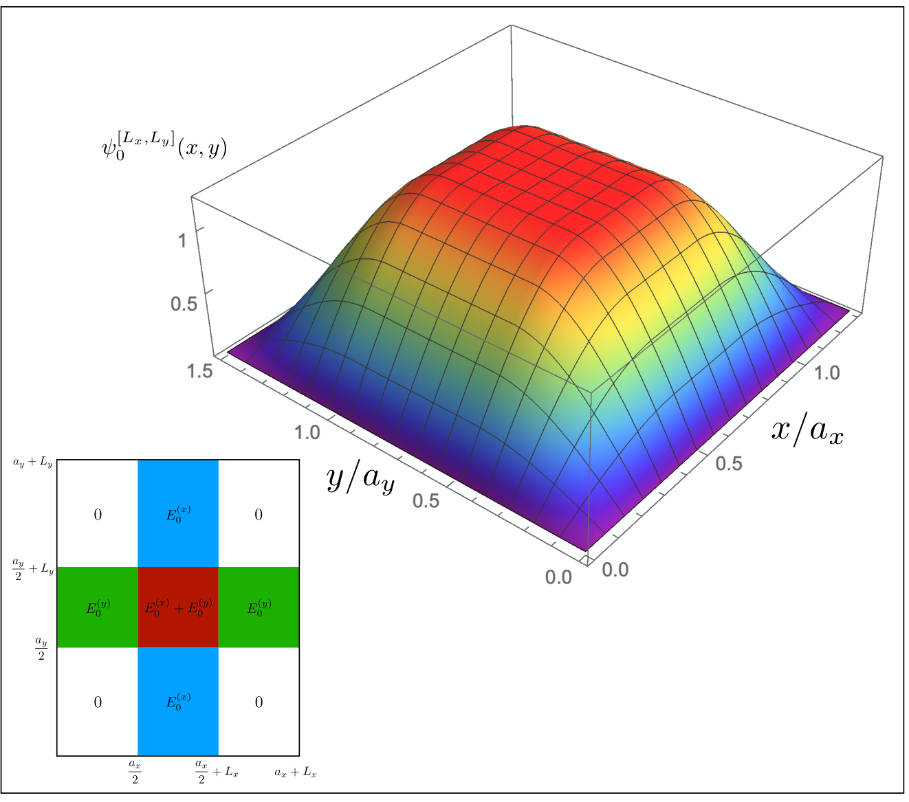
whose associated eigenenergies are $E_{0}^{(j)}=\frac{\hbar^{2}\pi^{2}}{2ma_{j}^{2}}$, so that $E_{0}=E_{0}^{(x)}+E_{0}^{(y)}$. From these expressions one immediately sees that the wave function $\psi_{0}(x,y)$ has zero gradient at the point $(\frac{a_{x}}{2},\frac{a_{y}}{2})$: we hence insert a potential box of height $E_{0}^{(x)}$ and width $L_{x}$ at the point $x=a_{x}/2$, and similarly a box of height $E_{0}^{(y)}$ and width $L_{y}$ at point $y=a_{y}/2$, obtainig the potential shown in the inset of Fig. 3. This new potential ground state eigenfunction reads:

$\displaystyle\psi_{0}^{[L_{x},L_{y}]}=\psi_{0}^{(x)[L_{x}]}(x)\psi_{0}^{(y)[L_{y}]}(y),$

(41)

where now $\psi_{0}^{(j)[L_{j}]}(j)$ is worth:

$\displaystyle\frac{1}{\sqrt{N_{j}}}\left\{\begin{array}[]{cc}\sin(\frac{\pi}{a_j}j)&\mbox{for $0\leq j\leq\frac{a_{j}}{2}$},\\ 1&\mbox{for $\frac{a_{j}}{2}\leq j\leq\frac{a_{j}}{2}+L_{j}$},\\ \sin(\frac{\pi}{a_j}(j-L_j))&\mbox{for $\frac{a_{j}}{2}+L_{j}\leq j\leq a_{j}+L_{j}$}.\end{array}\right.$

This leads to the ground state wave function plotted in Fig. 3, where one has a central region where $\psi_{0}^{[L_{x},L_{y}]}(x,y)$ is constant, and four regions where one of the components of the gradient is null. These four regions correspond to the blue and green regions of the inset of Fig. 3, where only one the kinetic components is absorbed into potential energy.

Extending this construction beyond the cases included in Eq. (32) is much more demanding due to the intrinsic interplay between the various coordinate components introduced by the seeding potential which prevents us from operating on one of them individually without affecting the others, leading in general to ambiguities affecting the boundary conditions which make not clear how to perform reverse engineering. It turns however that if we do restrict ourselves to small departure from the condition (32), approximate solutions can be found. To present this result we shall focus on a 2D geometry for which practical applications can be envisioned in the design of semiconductor electronic wave-guides. For this purpose let us consider a particle $A$ that moves on the $(x,y)$ plane under the action of a seeding potential which is translationally invariant along the longitudinal $y$ direction, i.e. $V(x,y)=V(x)$, hence writing (1) as

$$(\partial^{2}_{x}+\partial^{2}_{y})\psi_{E}({x,y})=-\frac{2m}{\hbar^{2}}(E-V({x}))\psi_{E}({x,y})\;.$$

(46)

The model clearly admits eigen-solutions of the form

$$\psi_{E}({x,y})=e^{iky}{\psi}_{n}(x)\;,\quad E=E_{n}+\hbar^{2}k^{2}/2m\;,$$

(47)

for $k$ real, and ${\psi}_{n}(x)$ being the $n$-th eigenstate of the 1D problem defined by $V(x)$ and associated with the eigenvalue $E_{n}$ (in what follows we shall assume this part of the spectrum to be discrete). Now considering $n=0$, i.e. identifying ${\psi}_{0}(x)$ and $E_{0}$ with the ground energy level associated with the 1D potential $V(x)$, let us consider the following modification of (46)

$$(\partial^{2}_{x}+\partial^{2}_{y})\psi_{E}({x,y})=-\frac{2m}{\hbar^{2}}(E-V^{[{L}(y)]}(x))\psi_{E}({x,y})\;,$$

(48)

where $V^{[{L}(y)]}(x)$ is obtained as in Eq. (II.1) when identifying the 1D seeding potential of that equation with the $V(x)$ appearing in Eq. (46), and where ${L}(y)$ is a (positive) smooth function of the longitudinal coordinate $y$. In what follows we shall consider the case where ${L}(y)$ varies only on a limited spatial interval $y\in{\cal I}:=[y_{in},y_{fin}]$, assuming the constant value $L_{in}:=L(y_{in})$ for $y\leq y_{in}$ and $L_{fin}:=L(y_{fin})$ for $y\geq y_{fin}$. For the special choice in which the two asymptotic values coincide (i.e. $L_{in}=L_{fin}=L$), and ${L}(y)$ is constant and the model retains its invariance under longitudinal translations ($V(x,y)=V^{[{L}]}(x)$): accordingly the solutions of (46) can be still obtained by separation of the coordinates through the ansatz

$$\psi_{E}({x,y})=e^{iky}{\psi}^{[L]}_{n}(x)\;,\quad E=E^{[L]}_{n}+\hbar^{2}k^{2}/2m\;,$$

(49)

where now ${\psi}^{[L]}_{n}(x)$ and $E_{n}^{[L]}$ are eigensolutions of the 1D problem characterized by the 1D potential $V^{[{L}]}(x)$. For $n=0$, Eq. (48) exhibits in particular a modification of $e^{iky}{\psi}_{0}(x)$ that, for all assigned $y$, is uniformly stretched along the transverse direction $x$, i.e. the wave-function

$$\psi_{E}(x,y)=e^{iky}\psi^{[{L}]}_{0}(x)\;,\quad E=E_{0}+\hbar^{2}k^{2}/2m\;,$$

(50)

that simply provides an instance of the construction we have anticipated at the beginning of the present section. The situation changes however when we allow for arbitrary choices of $L_{in}$ and $L_{fin}$. In this case clearly the above construction fails since the potential (48) will acquire an explicit dependence on $y$. Still a useful way to approaching the problem is to consider a modifed version of the ansatz (49)

$\displaystyle\psi_{E}(x,y)=e^{iky}{\tilde{\psi}(x,y)}\;,$

(51)

where now, apart from the phase term $e^{iky}$, we allow for a residual $y$-dependence in $\tilde{\psi}(x,y)$. By replacing this into (48) we get

$$\partial^{2}_{x}\tilde{\psi}(x,y)=-\frac{2m}{\hbar^{2}}\big[E-V^{[{L}(y)]}(x)\big]\tilde{\psi}(x,y)+\Delta(x,y)\;,$$

(52)

with

$\displaystyle\Delta(x,y):=-\partial^{2}_{y}\tilde{\psi}(x,y)-2ik\partial_{y}\tilde{\psi}({x,y})\;.$

(53)

We reconize that apart from the $\Delta(x,y)$ contribution, Eq. (52) reduces to Eq. (11) upon substituting $\tilde{\psi}({x,y})$ with $\psi_{E}({x})$. Accordingly one may try to use as an approximate solution of (52) the function $\psi^{[{L}(y)]}_{0}(x)$ obtained by evaluating the 1D wave-function of Eq. (II.1) for the stretching parameter ${L}(y)$, and taking for $E$ the corresponding ground state energy $E_{0}$, i.e.

$$\psi_{E}(x,y)\simeq e^{iky}\psi^{[{L}(y)]}_{0}(x)\;,\quad E\simeq E_{0}+\hbar^{2}k^{2}/2m\;.$$

(54)

This solution turns out to be appropriate as long as we can neglect the $\Delta(x,y)$ contribution into Eq. (52), a condition that, intuitively, can be ensured if ${L}(y)$ is a sufficiently slowly varying function with respect to $y$ on the whole interval ${\cal I}$ – see Appendix A for more details on this. Due to the presence of a non-constant stretching parameter $L(y)$, Eq. (54) represents a generalization of the stretched state (50) that applies for a model that, as anticipated, does not allow for trivial separation of variables.

Here we present few examples of the stretching mechanism for 1D models.

References

- (1) I. Liberal and N. Engheta, Nat. Photonics 11, 149 (2017).
- (2) R. W. Ziolkowski, Phys. Rev. E 70, 046608 (2004).
- (3) N. Engheta, Science 340, 286 (2013).
- (4) M. G. Silveirinha and N. Engheta, Phys. Rev. Lett. 97 157403 (2006)
- (5) B. Edwards, A. Alù, M. E. Young, M. G. Silveirinha and N. Engheta, Phys. Rev. Lett. 100, 033903 (2008).
- (6) B. Edwards, A. Alù, M. G. Silveirinha and N. Engheta, J. Appl. Phys. 105 044905 (2009)
- (7) S. Enoch, G. Tayeb, P. Sabouroux, N. Guerin and P. Vincent, Phys. Rev. Lett. 89 213902 (2002).
- (8) A. Alú, M. G. Silveirinha, A. Salandrino, and N. Engheta Phys. Rev. B 75, 155410 (2007).
- (9) V. Pacheco-Peña et al., Appl. Phys. Lett. 105, 243503 (2014).
- (10) C. Argyropoulos, P. Y. Chen, G. D’Aguanno, N. Engheta and A. Alú, Phys. Rev. B 85, 045129 (2012).
- (11) C. Argyropoulos, G. D’Aguanno and A. Alú, Phys. Rev. B 89, 235401 (2014).
- (12) H. Suchowski et al., Science 342, 1223 (2013).
- (13) R. Sokhoyan, and H. A. Atwater, Opt. Express 21, 32279 (2013).
- (14) J. B. Pendry, D. Schurig and D. R. Smith, Science 312, 1780 (2006).
- (15) D. Schurig et al., Science 314, 977 (2006).
- (16) L. Esaki and R. Tsu, IBM J. Res. Dev. 14, 61 (1970).
- (17) H. Kroemer, Rev. Mod. Phys. 73, 783 (2001)
- (18) C. W. J. Beenakker and H. van Houten, “Quantum transport in semiconductor nanostructures”, Solid State Physics 44, eds. H. Ehrenreich and D. Turnbull, New York Academic Press (1991).
- (19) L. P. Kouwenhoven, D. G. Austing and S. Tarucha, Rep. Prog. Phys. 64, 701 (2001).
- (20) S. M. Reimann and M. Manninen, Rev. Mod. Phys 74, 1283 (2002).
- (21) S. Datta, “Electronic transport in mesoscopic systems”, Cambridge University Press (1995).
- (22) M. G. Silveirinha and N. Engheta, Phys. Rev. Lett. 110, 213902 (2013)
- (23) S. Zhang, D. A. Genov, C. Sun, and X. Zhang, Phys. Rev. Lett. 100, 123002 (2008).
- (24) B. Liao, M. Zebarjadi, K. Esfarjani, and G. Chen, Phys. Rev. B 88, 155432 (2013).
- (25) S. Chesi and W. A. Coish, Phys. Rev. B 91, 245306 (2015).
- (26) N. I. Zheludev, Science 328, 582 (2010).
- (27) M. A. Castellanos-Beltran, K. D. Irwin, G. C. Hilton, L. R. Vale, and K. W. Lehnert, Nat. Phys. 4, 929 (2008).
- (28) M. G. Silveirinha and N. Engheta, Phys. Rev. B 86, 161104 (2012).
- (29) M. G. Silveirinha and N. Engheta, Phys. Rev. B 89, 085205 (2014).
- (30) R. Fleury and A. Alú, Phys. Rev. B 90, 035138 (2014).
- (31) A. Y. Cho and J. R. Arthur, Prog. Sol. State Chem. 10 157 (1975).
- (32) M. Abramowitz and I. A. Stegun, Handbook of Mathematical Functions with Formulas, Graphs, and Mathematical Tables. Applied Mathematics Series. 55 (December 1972).
- (33) J. C. W. Song and N. M. Gabor, Nat. Nanotechnol. 13, 986 (2018).
- (34) T . Bryllert, L-E. Wernersson, T. Löwgren and L. Samuelson Nanotech. 17, S227 (2006).
- (35) C. P. Svensson et al, Nanotech. 19, 305201 (2008).
- (36) S. Roddaro et al, Nanotech. 20, 285303 (2009).
- (37) D. Prete et al, Nano Lett. , 19 5, 3033 (2019).