On the behaviour of clamped plates under large compression
Abstract.
We determine the asymptotic behaviour of eigenvalues of clamped plates under large compression, by relating this problem to eigenvalues of the Laplacian with Robin boundary conditions. Using the method of fundamental solutions, we then carry out a numerical study of the extremal domains for the first eigenvalue, from which we see that these depend on the value of the compression, and start developing a boundary structure as this parameter is increased. The corresponding number of nodal domains of the first eigenfunction of the extremal domain also increases with the compression.
Key words and phrases:
Biharmonic operator, plate with tension, plate with compression, eigenvalues, asymptotics, extremal domains2010 Mathematics Subject Classification
Primary 35J30. Secondary 35P15, 35P20, 49R50, 74K201. Introduction
Let be a smooth bounded domain in , . We are interested in the following eigenvalue problem
| (1.1) |
considered as a model for a clamped plate. Here is a real parameter corresponding to the quotient between the tension and the flexural rigidity and, depending on its sign, represents whether the plate is under tension () or compression (). For domains as described above, the eigenvalues of (1.1) form an infinite sequence
where approaches as goes to infinity.
The study of this and similar problems has been considered in the literature continuously over time since the works of Lord Rayleigh [18] and Love [21] on clamped plates. We refer the reader to the book [15] for an extensive historical and scientific overview on the mechanics of plates through the Kirchhoff-Love model, which leads to problem (1.1).
In this paper, we are concerned with two issues related to (1.1), namely, the asymptotic behaviour of the eigenvalues as the parameter approaches (the case of was considered in [14]), and the extremal domains of such eigenvalues as varies. In the first instance, the above problem is closely related to
| (1.2) |
where now the eigenvalue parameter is , and the (positive) parameter stands for the elasticity constant of the medium surrounding the plate. We know from a result in [19] that for (1.2)
which when translated into the eigenvalue problem in (1.1) yields
Our main result along these lines is to extend this to all eigenvalues . This is achieved by a different approach from that used in [19], involving now a connection which, to the best of our knowledge, is new, between the eigenvalues of the clamped plate problem (1.1) and those of a Robin eigenvalue problem for the Dirichlet Laplacian in the case where is a ball – see Section 3 for the details. To be more precise, we prove the following
Theorem 1.1 (Asymptotic behaviour of the eigenvalue).
Let be a bounded domain in . Then, for any positive integer , the eigenvalues of (1.1) satisfy
| (1.3) |
as . Moreover,
| (1.4) |
as .
For positive values of , each of the eigenvalue curves is, in fact, made up of analytic eigenvalue branches which intersect each other - see Figure 1, where to illustrate this effect we plotted the quantity for the disk and for ellipses.
(a) 
 (b)
(b) 

This branch-switching phenomenon makes it much more difficult to obtain further terms in the asymptotic expansion and it is the independence of the first term on the order of the eigenvalue which allows us to derive the expansion for all . In the particular case where is a ball of radius , which is at the heart of the proof of Theorem 1.1, we are able to prove that the number of such eigenvalue branches which make up the eigencurve is finite, and we determine further terms in the asymptotic expansion of these analytic branches. These results are summarised in the following
Theorem 1.2 (Asymptotic behaviour of analytic eigenvalue branches for balls).
For any analytical branch of the eigenvalues of problem (1.1) when is a ball of radius , we have
| (1.5) |
as , where and are constants depending on the eigenvalue branch, with being positive. In the case of the first eigenvalue we have
It is possible to consider problem (1.1) with other boundary conditions, such as the Navier setting. This is not as interesting from a mathematical perspective, since the problem then reduces directly to the study of the second order elliptic operator . However, and as we show in Section 4, there is a major difference between the Dirichlet and Navier cases in that for the Navier problem the number of crossings of analytic branches to make up an eigencurve corresponding to the eigenvalue is actually infinite for each . Complex crossing and avoided-crossing patterns seem to be a characteristic of such systems in the large compression regime, and they have also been identified in the one-dimensional fourth-order problem with different boundary conditions studied in [11].
Concerning our second topic of study, namely extremal domains for eigenvalues of problem (1.1), even in the case where the parameter vanishes the problem is known to be extremely difficult with results available only in two and three dimensions – see [22, 5], respectively; for (1.2) there are no complete results in any dimension. Once is taken to be nonzero in (1.1), the only existing result is an extension to sufficiently small positive values of in two dimensions [4]. Our purpose in this part is thus mainly to provide a numerical exploration of the different types of extremal domains under an area restriction, showing in particular that the ball is no longer a minimizer for large compression.
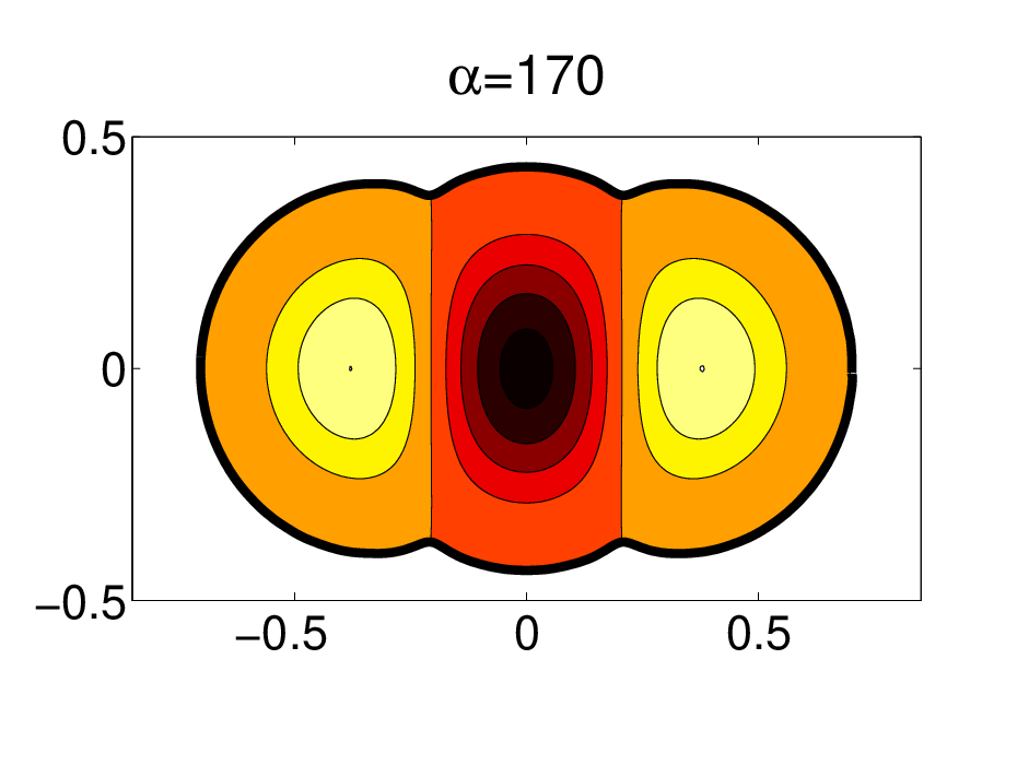
We consider the numerical solution of the eigenvalue problem (1.1) using the Method of Fundamental Solutions (see e.g., [1, 3]). This is a meshless numerical method where the approximation is made by a discretization of an expansion in terms of the single and double layer potentials. In particular, by construction, the numerical approximation satisfies the fourth-order partial differential equation and we can focus just on the approximation of the boundary conditions of the problem. The computational implementation of this numerical method is described in Section 6.1 and some numerical results for the shape optimization problem are presented in Section 6.3. In particular, we will study minimizers of the first eigenvalue of problem (1.1) subject to an area constraint. The obtained numerical results suggest that the minimizer depends on the parameter , with the ball being the minimizer for all negative and then extending to , for some positive . Note that this last result corresponds to that proved in [4] for sufficiently small , with our numerical simulations suggesting that, in fact, one may take to be at least as large as the first buckling eigenvalue. For large values of the parameter we obtain some non-trivial minimizers - see Figure 3.
This numerical study has been performed mainly among general simply connected domains. However, we performed also the optimization of the first eigenvalue of problem (1.1) among annuli having unit area and compared the optimal values that were obtained with the corresponding values of the ball. These results suggest that the first eigenvalue of the disk is always smaller than the corresponding eigenvalue of the optimal annulus, independently of the parameter .
2. Statement of the problem
We start by observing that problem (1.1) has the following weak formulation
| (2.1) |
and its eigenvalues may be described through their variational characterizations
| (2.2) |
In what follows, whenever the meaning is clear from the context, we will drop either argument in for the sake of simplicity.
In order to determine the eigenfunctions of problem (1.1) when , we rewrite equation (1.1) as
| (2.3) |
where
| (2.4) |
Both and are always real, as may be seen from inequality (4.6), and is always positive while the sign of depends on the sign of the eigenvalue .
For positive it is known that the solution of (2.3) can be written as (cf. [5])
| (2.5) |
where and are the Bessel and the modified Bessel functions, respectively, of the first kind of order , and are the spherical harmonic functions of order . The boundary conditions then yield the following system of equations
| (2.6) |
where we have set
Since we are interested in the existence of nontrivial solutions of system (2.6), we impose the corresponding determinant to be zero, namely
| (2.7) |
from which we obtain the corresponding eigenvalues and, as a consequence, the general form of the eigenfunctions. Using standard Bessel function identities, equation (2.7) may be rewritten as
| (2.8) |
When is strictly negative, then is strictly positive and, in place of (2.5), we now have
| (2.9) |
where the coefficients are given by a system similar to (2.6), and the eigenvalues are now solutions of
| (2.10) |
Finally, it remains to consider the case , which behaves in a slightly different way. We note that then while , and in particular this means that has to be an eigenvalue of the following buckling problem
| (2.11) |
for which the eigenfunctions are known to be of the form (they can be derived in a similar way as for the other cases)
| (2.12) |
In particular, has to be a solution of the following
| (2.13) |
Moreover, if is the -th eigenvalue of the buckling problem (2.11), we immediately deduce that the vanishing eigenvalue of problem (1.1) is exactly the -th one , and the multiplicity will be the same of .
3. Connection to the Robin Laplacian
Even though there are no simple relations between the Laplacian and the Bilaplacian in general (apart for the Navier problem (4.1)), if we consider the generic situation of problem (1.1) in the ball in with , we can draw a very precise connection to the Robin Laplacian.
To this end we recall that the Robin problem for the Laplace operator is as follows
| (3.1) |
For any real value of the corresponding spectrum consists of a non-decreasing sequence of eigenvalues with finite multiplicities diverging to plus infinity. In particular, for positive values of the eigenvalues are all strictly positive, while for the Robin problem (3.1) becomes the Neumann problem. It is also known that, as , problem (3.1) converges to the Dirichlet problem for the Laplace operator, namely
| (3.2) |
whose eigenvalues we will denote by
We recall that the eigenfunctions of (3.1) on a ball can be sorted out into three categories (cf. Section 2):
- i.
if the eigenvalue is positive, the eigenfunction is of the form
and eigenvalues are solutions of
- ii.
if the eigenvalue is negative, the eigenfunction is of the form
and eigenvalues are solutions of
- iii.
if the eigenvalue is zero, the eigenfunction is of the form , and in particular this occurs when .
At this point it is clear that any eigenfunction of the clamped plate problem (1.1) on the ball can be thought of as the sum of two different eigenfunctions of the Robin problem for the Laplacian (3.1). A first condition that these two Robin eigenfunctions have to satisfy is that their spherical parts coincide. This implies that they must come from two different eigenvalues and, in particular, we have that these two eigenvalues are and , and the multiplicities must coincide. Furthermore, such eigenfunctions must have the same index in their Bessel function part. Let us call two such eigenfunctions (with associated eigenvalues ) and let
i.e., we denote by the radial part. Since we want the boundary conditions in the clamped plate problem (1.1) to be satisfied, the only way to combine and is to set
| (3.3) |
as can be easily checked from the boundary conditions in the Robin problem for the Laplace operator (3.1). In particular, and must be Robin eigenfunctions associated with the same parameter . As for the equation, we observe that
and the equality is naturally satisfied since
| (3.4) |
On the other hand, letting go to infinity we get that, for specific values of and , we should consider eigenvalues of the Dirichlet Laplacian (3.2) instead. From the literature (see e.g., [8] and the references therein, and also [25] for a study of the first two Robin eigenvalues) we know that all the analytical branches related to the same Bessel function ( when the eigenvalue is negative, if zero) can be continued at generating a function which wraps around infinitely many times. If we call the -th eigenvalue associated with , then the analytical branches of eigenvalues of problem (1.1) are given by
| (3.5) |
for some , where the parameter is of no relevance here since any time reaches infinity has to be replaced by as
where is the -th eigenvalue of the Dirichlet problem for the Laplace operator (3.2) associated with . In particular, different branches of eigenvalues of the clamped plate problem (1.1) associated with the Bessel index are indexed by the parameter in (3.5). We remark that all the branches are of this type, hence no other branches are present. We sum up all these arguments in the following
Theorem 3.1.
Let and and be any two eigenfunctions of problem (3.1) in a ball associated with the eigenvalues and , respectively, and having the same spherical part, namely
Then the function defined in (3.3) is an eigenfunction of problem (1.1) in the ball associated with the eigenvalue and with the parameter .
This representation completely characterizes the analytic branch of the eigenvalue (for ) as the parameter varies. In the limits we have that the eigenvalue can be written as a product of eigenvalues of the Dirichlet problem for the Laplace operator (3.2), and the corresponding eigenfunction can also be written as a combination of eigenfunctions of problem (3.2).
In addition, all analytic branches of eigenvalues of the clamped plate problem (1.1) can be represented in this fashion.
Theorem 3.1 allows us to study the behaviour of the eigenvalues as . Actually, for the case , the convergence is well known in the literature for any smooth domain (see e.g., [14, p. 392]).
Theorem 3.2.
Let be the eigenfunction associated with , and suppose that there exists a point such that for any . Then
| (3.6) |
as , where is an eigenfunction of the Dirichlet problem for the Laplace operator (3.2) associated with .
We recall that, thanks to classical regularity theory for elliptic operators (cf.[15]), if then for any and, in particular, balls satisfy the hypotheses of Theorem 3.2. It is easily seen then that we can recover the first term of the asymptotics (3.6) using the known asymptotics for the Robin problem (see [26] and the references therein).
Regarding the asymptotics as , we compute it using the knowledge that for any given branch when we get to we obtain that both and can be expressed in terms of zeros of Bessel functions:
| (3.7) |
where is the -th zero of , whose asymptotic behaviour is known to be (cf. [23, formula (10.21.19)])
| (3.8) |
as .
Let us now denote by and two eigenfunctions of the Dirichlet problem for the Laplace operator (3.2) associated with and , respectively, having the same spherical part, and normalized such that is an eigenfunction of the clamped plate problem (1.1) under condition (3.7). Then using the Rayleigh quotient representation of we have
| (3.9) |
We recall that in this particular case we have , where we set for simplicity. We now compute the asymptotics for the remainder in (3.9) and get
telling us that . Going further we can get
and hence we have
Theorem 3.3.
We observe that, even if at a first glance the presence of the parameter may seem unnatural, it may be compared for example with the ordering number for zeros of Bessel functions . From this perspective, it is natural that it appears in formula (3.10).
We are now ready to prove Theorem 1.1.
Proof of Theorem 1.1.
In the case of a general domain , we shall denote the radius of the largest inscribed ball and that of the smallest ball containing by respectively. By the inclusion properties for problem (1.1), we know that any eigenvalue of is bounded from above and from below by the corresponding eigenvalues of the inscribed and circumscribed balls, respectively. This immediately proves (1.3). For higher eigenvalues it will, in general, be difficult to determine the precise order of each eigenvalue, but in the case of the first eigenvalue it is possible to identify the corresponding branch, namely that obtained by making and , and in turn obtain the following (asymptotic) expression
which implies (1.4). ∎
4. The Navier problem
We now turn our attention to the following eigenvalue problem
| (4.1) |
for any . We immediately notice the resemblance of the Navier problem (4.1) with problem (1.1), as its weak formulation reads
| (4.2) |
the only difference between this and (2.1) being the ambient space. In particular, comparing the variational characterization (2.2) of the eigenvalues of problem (1.1) with that of the eigenvalues of the Navier problem (4.1)
| (4.3) |
yields
Now we want to compute eigenfunctions and eigenvalues of the Navier problem (4.1). We can of course proceed as for the Dirichlet case in Section 2. However, we observe that we can modify the problem as follows
| (4.4) |
which tells us immediately that, if the domain has the cone property, the Navier operator in (4.4) is the square of the translated Dirichlet Laplace operator (cf. [15]). In particular, if we denote by the -th eigenvalue of the Dirichlet Laplacian (3.2), we get that the spectrum of (4.1) is given by
| (4.5) |
for any and for any (smooth enough) domain . We remark that, for (actually, for ) we have
for any , while on the other hand we actually have intersections of the branches (the intersection points will depend on ). However, we can still say that
that is
| (4.6) |
Theorem 4.1.
Let be a bounded open set in with the cone property. Then, for any
| (4.7) |
as . Moreover,
| (4.8) |
as .
Proof.
Equality (4.7) easily follows from the inequality chain (4.6) coupled with the asymptotic expansion (1.3).
As for (4.8), we first observe that
and for the choice we have
| (4.9) |
This alone is not enough to prove the asymptotic behaviour. However, we know that is a polygonal line and that each and every segment is tangent to the asymptotic curve (thanks to (4.9)). It is thus enough to show that the vertices have the same asymptotic behaviour, i.e., the points for which
or equivalently
therefore we have to show that
| (4.10) |
To this end we recall the Weyl asymptotics for the Dirichlet eigenvalue problem for the Laplacian (3.2), namely,
| (4.11) |
where and are (known) constants depending only on and the dimension . From the binomial Taylor expansion
we have
| (4.12) |
which clearly goes to zero for larger than one. ∎
Remark 4.2.
If the domain is not bounded, it is still possible to prove (4.8) without using the asymptotics (1.3) while following the same strategy we used in the previous proof. In particular, in order to get the term , it suffices to show that
which follows from the equality
and the fact that the ratio of consecutive eigenvalues converges to , thanks to Weyl’s asymptotics (4.11).
Remark 4.3.
We observe that the behaviour of the clamped plate problem (1.1) and that of the Navier problem (4.1) are substantially different. On the one hand, from the asymptotics (3.10) we have that the branches of eigenvalues of the clamped plate problem (1.1) will stop intersecting for some sufficiently large value of , at least in the case of balls where the parameters and provide a clear ordering of the branches, so that it is in principle possible to see which branch will eventually be the -th eigenvalue. On the other hand, we know a priori that the branches of eigenvalues of the Navier problem (4.1) will have an infinite number of intersections, making it quite complicated to decide which is the -th eigenvalue. In particular, the knowledge of the behaviour of each individual branch does not provide sufficient information on the asymptotics of the eigenvalues. Similarly, even though the eigenspaces do not depend on , that associated with the eigenvalue will keep on changing, creating a strange phenomenon of non-convergence.
5. Shape derivatives
We will now consider the problem of finding extremal domains for the -th eigenvalue of problem (1.1), namely,
Problem 1.
Determine
We observe that proving existence for Problem 1 within a specific class of domains can be quite difficult and, to the best of our knowledge, there are no results available in general. To gauge the difficulties involved, we refer the reader to [7] for a survey on existence results for the Laplacian case, for which it is still not known if existence holds within the class of open sets.
We will focus now on Problem 1 with . We begin by deriving the formula for the Hadarmard shape derivative of an eigenvalue of (1.1). Note that the formula in the case was already derived in a general setting and for multiple eigenvalues, see [10, 24]. We also refer to [9] and the references therein for a complete discussion on Hadamard formulas for the Biharmonic operator, also in the case . Nevertheless, for the sake of simplicity we show here how to derive it in our specific case.
Consider an application such that is differentiable at 0 with , where is the set of bounded Lipschitz maps from into itself, is the identity and is a given deformation field.
We will use the notation , for a given set , , is an associated eigenfunction with unitary norm, and will denote the derivative of at . Moreover, we assume that is simple.
It is well known (see e.g., [13]) that if we define
for some function , then the Hadamard shape derivative is given by
| (5.1) |
As a consequence we have
Theorem 5.1.
Let be a bounded open set of class . The Hadamard shape derivative for a simple eigenvalue of problem (1.1) with corresponding eigenfunction is given by
| (5.2) |
Proof.
We have
| (5.3) |
and the eigenfunction is normalized,
| (5.4) |
The function can be calculated by solving the following boundary value problem (c.f. [16, 17])
| (5.5) |
Since the case can be recovered from [24] (and can be done similarly to what follows), we assume and the eigenvalue equation can be written as
so that we have
| (5.6) |
Applying now formula (5.1) to the equation (5.3) and using (5.6) we obtain
The proof is concluded once we observe that (cf. [15]), and since on , we have that
∎
Remark 5.2.
Using formula (5.2), we may try to attack Problem 1 via the Lagrange Multiplier Theorem. Since the constraint here is , we obtain the following condition
| (5.7) |
Note that condition (5.7) has then to be added to problem (1.1), yielding an overdetermined problem resembling the Serrin problem (see [27]). However, problem (1.1) coupled with condition (5.7) is a more difficult problem, and the only partial result available in the literature can be found in [12].
It is worth observing that solving the overdetermined problem (1.1), (5.7) is not equivalent to solving Problem 1: in fact, the former provides just a critical point, that may be only a local minimizer, or even a local maximizer. Interestingly enough, though, eigenfunctions on the ball always satisfy condition (5.7). For a more detailed analysis of this fact, we refer to [9, 10].
6. Numerical Methods
6.1. Numerical solution of the eigenvalue problem
In this section we will describe a numerical method for solving (1.1).
A fundamental solution of the partial differential equation of the eigenvalue problem (1.1) is given by (see e.g., [20])
| (6.1) |
where is a Hankel function of the first kind.
We will consider particular solutions of the partial differential equation of the eigenvalue problem (1.1), by defining the boundary integral operators
where is an artificial boundary that surrounds (see e.g., [1, 3]), and and are densities. The numerical approximation of an arbitrary solution of the PDE of the eigenvalue problem (1.1) can be justified by density results e.g., [1, 2]. Moreover, we will assume that does not intersect . Thus, we can discretise the boundary integral operators by considering the linear combinations
| (6.2) |
where are some points on Note that the functions are particular solutions of the partial differential equation involved in the eigenvalue problem (1.1) and the coefficients can be determined by fitting the boundary conditions of the problem.
We consider some collocation points , (almost) uniformly distributed on and impose the boundary conditions of the problem which leads to the system
| (6.3) |
We will consider the choice for source points described in [1], assume that , and denote this vector simply by . Using the notation , the system (6.3) can be rewritten as
| (6.4) |
The approximations of the eigenvalues can be calculated by adapting the Betcke-Trefethen method (see [6]) to this context. We consider points , randomly chosen in and define the following six blocks
where . Then, we define the matrix
compute the decomposition of , and calculate the minimal eigenvalue of the first block of the matrix that will be denoted by . The approximations for the eigenvalues of problem (1.1) are the values , for which .
6.2. Numerical shape optimization
In this section we will consider the shape optimization Problem 1 among general simply connected planar domains, whose boundary can be parametrized by
for some continuous and -periodic functions and . We will consider the (truncated) Fourier expansions
and
for a sufficiently large , and the optimization procedure consists in finding optimal coefficients , , , . The optimization is performed by a gradient-type method, using the Hadamard shape derivative given by Theorem 5.1 to calculate the derivative of the eigenvalue with respect to perturbations of the coefficients , , , .
6.3. Numerical results
In this section we present the main results that we gathered with our numerical procedure for solving Problem 1.
As was mentioned in the Introduction, each of the eigenvalue curves is made up of analytic eigenvalue branches which intersect each other. We illustrate this fact in Figure 1. As was shown in Theorem 1.1, all the eigenvalues have the following asymptotic behaviour
Thus, in order to produce more convenient pictures, instead of plotting the first eigenvalues as functions of , we will extract the first term of the expansion, which is the same for all eigenvalues, i.e., in Figure 1 we plot the quantities
for a disk of unit area and similar results for an ellipse with unit area and eccentricity equal to .
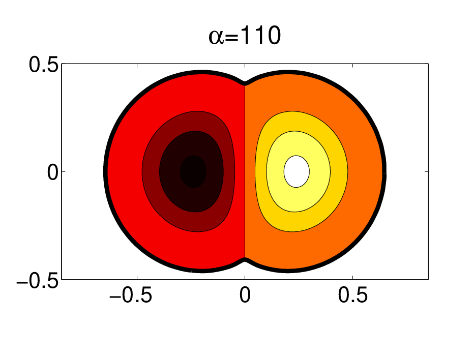
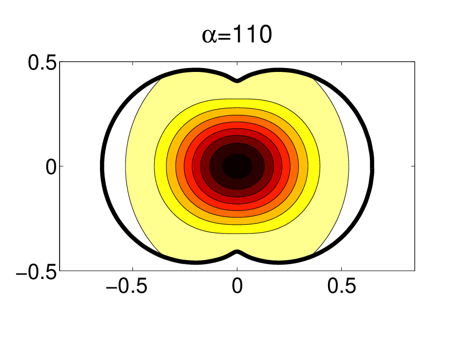
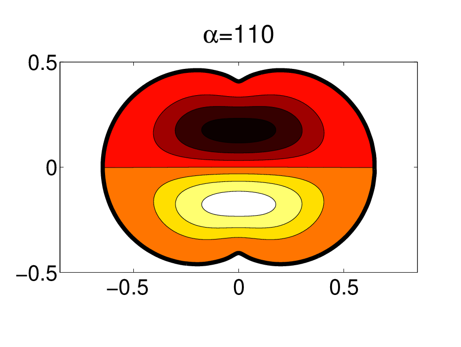
Figure 2 shows the curve of the quantity . We can observe several branches corresponding to different types of minimizers. Some of them, obtained for , are plotted in Figure 3. The optimal eigenvalue is the minimum among the values obtained for all the branches. We calculated the critical value of , which is the maximal value of for which the ball is the minimizer and obtained . In [4] it was proved that the ball is the minimizer for for some , where is the first buckling eigenvalue of the disk with unit area. Our numerical results suggest that actually the result may be true for a larger range of values of and we conjecture that the ball is the minimizer for . On the other hand, we have numerical evidence to support the conjecture that for , the ball is no longer the minimizer. For instance, for , the first eigenvalue of the ball of unit area can be directly calculated by solving (2.9) and is equal to -1622.16613… In Table 1 we show some numerical approximations for the first eigenvalue of the minimizer that we obtained with our algorithm when , which is plotted in Figure 3, for different values of . These results suggest that the first eigenvalue of this domain is equal to -1786.35377…, which is significantly smaller than the first eigenvalue of the disk.
| 1000 | -1786.3537774 |
|---|---|
| 1500 | -1786.3537779 |
| 1800 | -1786.3537762 |
| 2000 | -1786.3537753 |

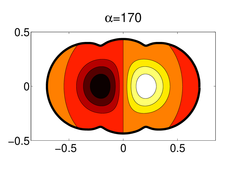
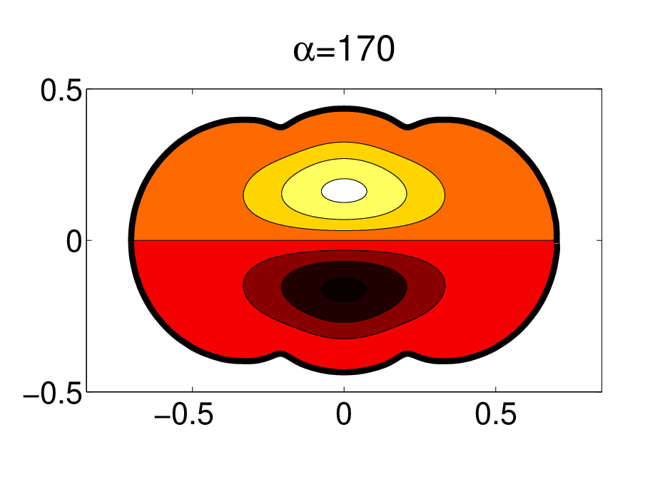
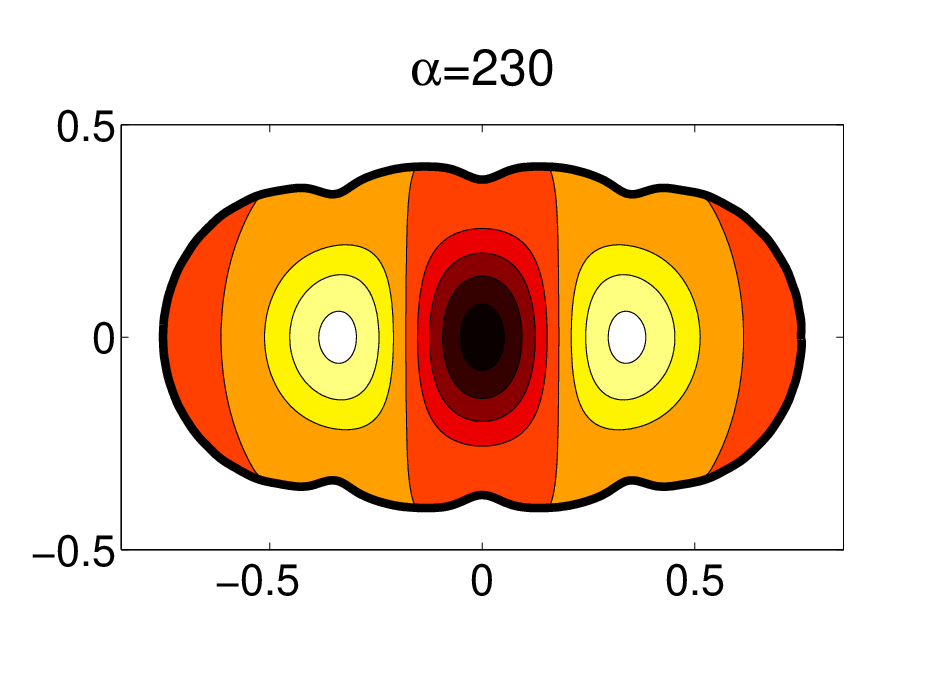
In Figure 5 we plot the eigenfunctions associated to the first three eigenvalues of the optimizers of , obtained for . In this work we considered just the optimization of the first eigenvalue. However, we observed that, besides the fact that the eigenfunction associated with the first eigenvalue changes sign, it also has different number of nodal domains, depending on the parameter . Moreover, ’similar’ eigenfunctions appear associated with eigenvalues of different orders. For instance, the eigenfunction associated with the first eigenvalue for is antisymmetric with respect to the first axis. However, the eigenfunction associated with the first eigenvalue for is symmetric with respect to the first axis and the first antisymmetric eigenfunction with respect to the first axis is associated not with the first eigenvalue, but with the second eigenvalue.


Figure 4 shows a zoom of the boundary of the optimizer obtained numerically for , in a neighbourhood of the re-entrant part of the boundary. Note that the boundary of the domains considered in the optimization procedure was parameterized by a (truncated) Fourier expansion. In particular the domains considered are always smooth and it is not clear how to obtain information on the regularity of the boundary of the optimizer from this. In particular, it is not possible to deduce whether this corresponds to a smooth boundary, a corner, or even a cusp.



Acknowledgements
This work was partially supported by the Fundação para a Ciência e a Tecnologia (Portugal) through the program “Investigador FCT” with reference IF/00177/2013 and the project Extremal spectral quantities and related problems (PTDC/MAT-CAL/4334/2014). Most of the research in this paper was carried out while the second author held a post-doctoral position at the University of Lisbon within the scope of this project. The second author is a member of the Gruppo Nazionale per l’Analisi Matematica, la Probabilità e le loro Applicazioni (GNAMPA) of the Istituto Nazionale di Alta Matematica (INdAM).
References
- [1] C. J. S. Alves and P. R. S. Antunes, The Method of Fundamental Solutions applied to the calculation of eigensolutions for 2D plates, SIAM Journal on Matrix Analysis and Applications, 77 (2009), pp. 177–194.
- [2] P. R. S. Antunes, On the buckling eigenvalue problem, Journal of Physics A: Mathematical and Theoretical, 44 (2011), p. 215205.
- [3] P. R. S. Antunes, Optimal Bilaplacian eigenvalues, SIAM Journal on Control and Optimization, 52 (2014), pp. 2250–2260.
- [4] M. S. Ashbaugh, R. Benguria, and R. Mahadevan, A sharp lower bound for the first eigenvalue of the vibrating clamped plate problem under compression, preprint, (2018).
- [5] M. S. Ashbaugh and R. D. Benguria, On Rayleigh’s conjecture for the clamped plate and its generalization to three dimensions, Duke Math. J., 78 (1995), pp. 1–17.
- [6] T. Betcke and L. N. Trefethen, Reviving the Method of Particular Solutions, SIAM Rev., 47 (2005), pp. 469–491.
- [7] D. Bucur, Existence results. In: Shape Optimization and Spectral Theory, ed. A. Henrot, De Gruyter Open, Warsaw/Berlin, 2017.
- [8] D. Bucur, P. Freitas, and J. B. Kennedy, The Robin problem. In: Shape Optimization and Spectral Theory, ed. A. Henrot, De Gruyter Open, Warsaw/Berlin, 2017.
- [9] D. Buoso, Analyticity and criticality results for the eigenvalues of the biharmonic operator. In: Geometric properties for parabolic and elliptic PDE’s, Springer Proc. Math. Stat., 176, Springer, 2016.
- [10] D. Buoso and P. D. Lamberti, Eigenvalues of polyharmonic operators on variable domains, ESAIM Control Optim. Calc. Var., 19 (2013), pp. 1225–1235.
- [11] L. M. Chasman and J. Chung, Spectrum of the free rod under tension and compression, Applicable Anal.
- [12] R. Dalmasso, Un problème de symétrie pour une équation biharmonique, Ann. Fac. Sci. Toulouse Math., 11 (1990), pp. 45–53.
- [13] M. C. Delfour and J.-P. Zolésio, Shapes and Geometries: Analysis, Differential Calculus, and Optimization, Adv. Des. Control 4, SIAM, Philadelphia, 2001.
- [14] L. S. Frank, Coercive singular perturbations: eigenvalue problems and bifurcation phenomena, Ann. Mat. Pura Appl., 148 (1987), pp. 367–395.
- [15] F. Gazzola, H.-C. Grunau, and G. Sweers, Polyharmonic boundary value problems. Positivity preserving and nonlinear higher order elliptic equations in bounded domains, Lecture Notes in Mathematics, 1991, Springer-Verlag, Berlin, 2010.
- [16] P. Grinfeld, Hadamard’s formula inside and out, Journal of Optimization Theory and Applications, 146 (2010), pp. 654–690.
- [17] A. Henrot and M. Pierre, Variation et optimisation de formes. Une analyse géométrique, Springer, Series Mathématiques et Applications, Vol. 48, 2005.
- [18] B. R. J. W. Strutt, The Theory of Sound, Dover Publications, New York, 2nd ed., 1945.
- [19] B. Kawohl, H. A. Levine, and W. Velte, Buckling eigenvalues for a clamped plate embedded in an elastic medium and related questions, SIAM J. Math. Anal., 24 (1993), pp. 327–340.
- [20] M. Kitahara, Boundary integral equation methods in eigenvalue problems of elastodynamics and thin plates, Elsevier, Amsterdam, 1985.
- [21] A. Love, A treatise on the Mathematical Theory of Elasticity, Dover Publications, New York, 4th ed., 1944.
- [22] N. S. Nadirashvili, Rayleigh’s conjecture on the principal frequency of the clamped plate, Arch. Rational Mech. Anal., 129 (1995), pp. 1–10.
- [23] F. W. J. Olver, D. W. Lozier, R. F. Boisvert, and C. W. Clark, eds., NIST handbook of mathematical functions, Cambridge University Press, Cambridge, 2010.
- [24] J. Ortega and E. Zuazua, Generic simplicity of the spectrum and stabilization for a plate equation, SIAM J. Cont. Optim., 39 (2001), pp. 1585–1614.
- [25] P-Freitas and R. Laugesen, From Neumann to Steklov via Robin: the Weinberger way, 2018, https://arxiv.org/abs/1810.07461.
- [26] K. Pankrashkin and N. Popoff, Mean curvature bounds and eigenvalues of robin laplacians, Calc. Var. Partial Differential Equations, 54 (2015), pp. 1947–1961.
- [27] J. Serrin, A symmetry problem in potential theory, Arch. Rational Mech. Anal., 43 (1971), pp. 304–318.