Ultracontractive Properties for Directed Graph Semigroups with Applications to Coupled Oscillators
Abstract
It is now well known that ultracontractive properties of semigroups with infinitesimal generator given by an undirected graph Laplacian operator can be obtained through an understanding of the geometry of the underlying infinite weighted graph. The aim of this work is to extend these results to semigroups with infinitesimal generator given by a directed graph Laplacian operator, through an analogous inspection of the geometry of the underlying directed graph. In particular, we introduce appropriate nomenclature to discuss the geometry of an infinite directed graph, as well as provide sufficient conditions to extend ultracontractive properties of undirected graph Laplacians to those of the directed variety. Such directed graph Laplacians can often be observed in the study of coupled oscillators, where recent work in [2] made explicit the link between synchronous patterns to systems of identically coupled oscillators and ultracontractive properties of undirected graph semigroups. Therefore, in this work we demonstrate the applicability of our results on directed graph semigroups by extending the aforementioned investigation beyond the idealized case of identically coupled oscillators.
1 Introduction
The study of heat equations on graphs have long been a topic of inquiry which has successfully related the geometric properties of the underlying graph to time-dependent estimates of the behaviour of the semigroup generated by the associated graph Laplacian [7, 11, 12, 13]. A discrete heat equation takes the form of the linear ordinary differential equation
| (1.1) |
for each . Here denotes the derivative of with respect to the independent variable , is the countably infinite vertex set of an underlying graph, and represents the weight of the edge from vertex to vertex .11 1 This will be made more precise in the following section. In the case of undirected (or symmetric) graphs, much work has been done to connect the behaviour of a random walk on the underlying graph to the long-time dynamics of solutions to the differential equation (1.1) associated to the graph [2, 7, 10, 19]. This work has successfully introduced ultracontractive properties into the study of heat kernels on symmetric graphs, thus continuing a long investigation into decay of one-parameter semigroups which dates back at least to the seminal work of Varopoloulus [21].
It appears that the study of discrete heat equations on graphs is greatly skewed towards undirected graphs, with few results pertaining to ultracontractive properties of system (1.1) associated with a directed graph. Therefore, it is the intention of this manuscript to introduce a set of sufficient conditions which allow one to obtain ultracontractive properties of the semigroup generated by the linear operator governing the right-hand side of (1.1), based upon the geometry of the underlying directed graph. Precisely, in this manuscript a set of sufficient conditions is provided for graphs of dimension two and up which can guarantee that the ultracontractive properties from undirected graphs can be extended to the general setting of directed graphs. These ultracontractive properties are equivalent to the uniform decay in of solutions to (1.1) over various Banach spaces of real sequences indexed by the vertex set .
Aside from their connection with random walks, discrete heat equations of the form (1.1) arise naturally in the study of coupled oscillators, where the stability of a synchronous state is often understood via the geometry of an associated graph. Although this connection has been well-studied in the finite-dimensional setting [4, 8], there still remain a number of open problems pertaining to the infinite-dimensional setting. Recent work has initiated the investigation into the connection between graph geometry and stability in infinite systems of coupled oscillators by restricting the investigation to identically coupled oscillators [2]. This restriction to identically coupled oscillators lacks the generality that is already well understood in the finite-dimensional setting, and therefore in this manuscript we aim to describe how our work on system (1.1) can be used to extend the results of [2] beyond such an idealized scenario. Therefore, our work herein leads to a more robust result detailing sufficient conditions for the stability of infinitely-many coupled oscillators.
Systems of the form (1.1) have also been documented in the study of the stability of traveling wave solutions to lattice dynamical systems [15]. This investigation required a tedious analysis using the Fourier transform to obtain decaying bounds on an associated Green’s function, which was then used to infer linearized stability of an associated ordinary differential equation. It is therefore the intention of this work to provide a framework in which future investigations into the stability of solutions to lattice dynamical systems can readily obtain linearized stability through a careful checking of the conditions on (1.1) laid out in this manuscript, potentially reducing the amount of difficulty required to obtain decaying bounds on a Green’s function. Hence, it has become a long-term goal to apply the results of this work to the diverse and expanding study of stability in lattice dynamical systems.
This manuscript is organized as follows. In Section 2 we introduce the proper nomenclature, notation, and hypotheses to discuss discrete heat equations on graphs, as well as introduce some new notation to properly analyze directed graphs. Then, in Section 3 we discuss some of the known results for undirected graphs, as well as provide some necessary extensions of this work which will become useful when discussing directed graphs. Our main result is Theorem 4.1 in Section 4 which provides a set of sufficient conditions on the geometry of a directed graph to obtain uniform decay of solutions to (1.1). Section 5 is dedicated to demonstrating the importance of Hypothesis 2, which forms the major assumption on the geometry of the directed graphs considered in this manuscript. An example of a system of the form (1.1) is provided for which this assumption fails and it is shown that the decay of solutions cannot be understood via the methods outlined in this manuscript. Finally, in Section 6 we connect these results to the stability of coupled oscillators, resulting in Theorem 6.1, which is supplemented by a brief discussion of an application of this theorem.
2 Definitions and Hypotheses
We consider a graph with a countably infinite collection of vertices, , and a set of oriented edges between these vertices, . If there exists an edge originating at vertex and terminating at vertex then we will write , but we note that since the edges are assumed to be oriented the relation is not necessarily symmetric. Furthermore, we may equivalently consider the set of edges as a subset of the product by writing if there exists an edge originating at vertex and terminating at vertex . A graph is called strongly connected (or simply connected in this manuscript) if for any two vertices there exists a finite sequence of vertices in , , such that , , , . We will only consider connected graphs for the duration of this work.
We will also consider a weight function on the edges between vertices, written , such that for all we have if and only if . This then leads to the notion of a weighted oriented graph, written as the triple . We emphasize that is not necessarily symmetric with respect to its arguments, even in the case when and for some . Moreover, it should be noted that in the interest of full generality we have not assumed that the weights are nonnegative, but only that all edges must have a nonzero weight. The weight function further allows us to consider the graph Laplacian (sometimes combinatorial graph Laplacian) associated to the graph given by the linear operator, , acting on the real sequences by
| (2.1) |
so that (1.1) can be written abstractly as the linear ordinary differential equation , upon suppressing the dependence on the independent variable for convenience. Hence, the general solution to (1.1) with initial condition can be written , where is the semigroup with infinitesimal generator . It will therefore be our goal in this manuscript to obtain ultracontractive properties on the semigroup , which are equivalent to determining uniform decay properties of the solution .
Natural spatial settings for the graph Laplacian operator are the real sequence spaces
| (2.2) |
for any . The vector space becomes a Banach space when equipped with the norm
| (2.3) |
We may also consider the Banach space , the vector space of all uniformly bounded real sequences indexed by with norm given by
| (2.4) |
It should be noted that these definitions extend to any countable index set , independent of a respective graph.
The potential asymmetry of the edges and weights on the graph make the direct application of results for graphs with undirected edges unlikely, and therefore we wish to develop a method of extending these results to the setting of (1.1) for a general directed graph. Let us begin by defining the function by
| (2.5) |
so that for all . Similarly, we will define the function by
| (2.6) |
so that for all . Hence, one sees that
for all . This leads to the following definition.
Definition 2.1.
The graph Laplacian (2.1) induces the linear operators and given by
| (2.7) |
and
| (2.8) |
We refer to as the symmetric graph Laplacian induced by , and as the skew-symmetric graph Laplacian induced by .
It should immediately be noted that . Moreover, the function and the linear operator also leads to the definition of an underlying undirected weighted graph.
Definition 2.2.
The symmetric graph induced by , denoted , is the graph with vertex set and edge set, , defined by assigning an undirected edge connecting if and only if .
The graph becomes a weighted graph when considered with the symmetric weight function . Therefore, it will be through the graph and the associated symmetric graph Laplacian that we will work to understand decay properties of the linear equation (1.1). We present the following hypothesis which is fundamental to our interpretation of , and in turn .
Hypothesis 1.
The graph satisfies the following:
- 1.
The function is nonnegative, and furthermore if , then .
- 2.
There exists a constant such that for all .
- 3.
The set is such that there exists a constant such that for all .
Hypothesis 1 first details that all edge weights of are strictly positive. We should note that this does not contradict our assumption that the weight function associated with the original directed graph can assume negative values. Indeed, we simply have imposed that if , then we necessarily have and . This also leads to our second assumption in Hypothesis 1 which details that the graph essentially takes all edges in , makes them unoriented, and assigns a weight which is the average of the directed edge weights between each pair of vertices. Hence, we have assumed that the creation of does not disconnect two vertices, and since was assumed to be connected, we therefore have that is also connected.
Hypothesis 1 further details that we assume the edge weights to be uniformly bounded above, and that each vertex in is connected to a finite number of vertices. When a graph exhibits this latter property, it is often said to be locally finite. It should be noted that our assumption is slightly more restrictive than just being locally finite though, as we have assumed that the number of vertices each vertex is connected to is uniformly bounded from above. The set represents the neighbourhood of in the graph . In the context of the directed graph , under Hypothesis 1 we have that represents the set of all vertices for which or . It will be through Hypothesis 1 that we will work to understand the decay of solutions to the linear equation (1.1).
We now turn to the skew-symmetric graph Laplacian and the associated weight function . Let us define the quantity
| (2.9) |
This leads to the following hypothesis.
Hypothesis 2.
The quantity defined in (2.9) is finite.
We remark that we make no assumption on the exact magnitude of , we simply assume that it is finite. This implies that for any , the weights and will be -close for infinitely many . In Section 5 we demonstrate that in the absence of Hypothesis 2 solutions to (1.1) cannot necessarily be understood through the geometry of the associated symmetric graph. We conclude this section with the following simple example which illustrates all of the definitions and hypotheses put forth in this section.
Example 1.
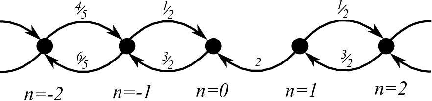
Consider a directed graph with index set with edges from vertices to and vice-versa, except that there is no edge from vertices indexed by to . The edge weights are given by
for all , where we note that meaning that there is no edge from to . Figure 1 provides a visual representation of this graph. The important point here is that for large we have that the weights and become uniformly close together at a rate of , which will guarantee that Hypothesis 2 is indeed satisfied.
Then, using the definition of and above we get that
for all , along with the symmetry conditions and . The graph is simply the standard one-dimensional integer lattice, where successive integers are connected by an undirected edge of weight . Hence, it is very easy to check that Hypothesis 1 does indeed hold for . Moreover, the quantity in this case is given by
where is the hyperbolic cotangent function. Hence, in this case, and hence Hypothesis 2 holds for this graph as well.
3 Ultracontractive Properties for Undirected Graphs
In this section we provide a review of the relevant results for undirected graphs. We will see that an understanding of the geometry of the graph can be used to obtain uniform decay of solutions to the linear ordinary differential equation
| (3.1) |
It should be noted that much of the information in this section comes as a review of the work in [2], and many of the graph theoretic facts and definitions can be found in, for example, [7, 19]. Hence, in this section we provide assumptions that lead to the algebraic decay of solutions to (3.1), which will be utilized in the following section to obtain algebraic decay of solutions to (1.1).
We begin by defining the measure of a vertex of the graph , written , and defined by
| (3.2) |
We note that Hypothesis 1 dictates that , for all , and hence the measure is well-defined. This notion extends to the volume of a subset, , by defining
| (3.3) |
Hence, we see that can be interpreted as a measure space with -algebra given by the power set of .
Connected undirected graphs also have a natural metric associated to them, here denoted , which returns the smallest number of edges needed to traverse from one vertex to another. This metric allows for the consideration of a ball of radius centred at the vertex , denoted by
| (3.4) |
For simplicity we will simply write to denote . The combination of the graph metric and the vertex measure allows one to interpret a weighted graph as a metric-measure space.
We now provide a series of definitions to describe the geometry of .
Definition 3.1.
The weighted graph satisfies a uniform polynomial volume growth condition of order , abbreviated VG(d), if there exists and such that
| (3.5) |
for all and .
The value in Definition 3.1 is often referred to as the dimension of the graph . A potential reason for this is that the characteristic examples of graphs satisfying VG(d) are the integer lattices with an edge between two vertices if and only if , and all edge weights taken to be identically [1]. In Example 1 we saw that the resulting symmetric graph is exactly of this type, and therefore it satisfies VG(1). It should be noted that need not be an integer, as one may construct fractal graphs which satisfy VG(d) for non-integer valued . For the duration of this work we will restrict our attention to , since the methods of Section 4 fail when .
Definition 3.2.
We say satisfies the local elliptic property, denoted , if there exists an such that
| (3.6) |
for all and .
It was pointed out in [2, Lemma ] that a sufficient condition to satisfy this local elliptic property, , is to have the edge weights, , bounded above and below by positive constants for all , and to have a uniform upper bound on the number of elements in over . Of course, Hypothesis 1 takes care of two thirds of these sufficient conditions, but in the interest of generality we refrain from assuming the third and final condition, as these conditions were not found to be necessary.
Definition 3.3.
The weighted graph satisfies the Poincaré inequality, abbreviated PI, if there exists a constant such that
| (3.7) |
for all real sequences , all , and all , where
| (3.8) |
It is immediately apparent that proving an undirected graph satisfies the Poincaré inequality is a significant analytical undertaking. Some methods were outlined in [6], and in [2] the notion of a rough isometry was introduced to demonstrate that a graph satisfies PI. We refrain from going into further detail here, but direct the reader to those sources for a full analytical treatment of the Poincaré inequality with regards to undirected graphs.
It is well-known [17, 18, 22] that is the infinitesimal generator of the semigroup . Moreover, the semigroup acts on the real sequences by
| (3.9) |
where are transition probabilities generated by a random walk on the weighted graph [7, 17, 22] (see [2] for complete details). This leads to the following proposition, which summarizes the work of [2, Section ].
Proposition 3.4 ([2], §3.3).
Assume that satisfies Hypothesis 1, , PI, and VG(d) for some . Then, there exists a constant such that
| (3.10) |
for all and real sequences .
We now provide an extension of Proposition 3.4, which will be integral to our work here. Let us begin by defining the functions
for all and
It is easy to see that for each the functions satisfy for all , and are semi-norms on for each . Furthermore, since is assumed to be connected, it follows that the vanish if and only if is a constant sequence. The components are typically interpreted as the discrete analogue of a directional derivative of the sequence in the direction of the edge . Hence, can be thought to be the -norm of the (discrete) gradient of the sequences in . We now provide the following lemma which extends the bounds of Proposition 3.4.
Lemma 3.5.
Assume that satisfies Hypothesis 1, , PI, and VG(d) for some . There exists constants such that for all we have
for all and .
Proof.
It was shown by Delmotte that any graph satisfying , PI, and VG(d) for some , must also satisfy a Parabolic Harnack Inequality [7], which we do not explicitly state here because it will not be necessary to our result. But, the work of [14, Theorem ] dictates that any graph (or more generally metric space) satisfying the Parabolic Harnack Inequality further satisfies the estimate
for all and some independent constants . Hence, assuming Hypothesis 1, for all and we have
since because .
Then, using the form for given in (3.9), for all , , and we have
This therefore implies that
for all since for all . Then, from Proposition 3.4 we have that
for some constant , where we have introduced the notation . This then gives that
which proves the cases with . The case follows in a nearly identical fashion, and is therefore omitted. This completes the proof. ∎
4 Ultracontractive Properties for Directed Graphs
In this section we show that an understanding of the graph and its associated symmetric graph Laplacian can be used to understand the decay of solutions to (1.1). The following theorem is our main result on the decay of solutions to (1.1), and its proof will be broken up into a series of lemmas throughout this section.
Theorem 4.1.
Consider the linear ordinary differential equation (1.1), and construct and as defined in Definition 2.1 and 2.2, respectively. Assume that satisfies Hypothesis 1, , PI, and VG(d) for some and that Hypothesis 2 is true. Then, there exists a continuous, positive, strictly increasing function and a constant such that for all we have that the solution to (1.1) satisfies the following decay estimates:
| (4.1) |
for all and .
Remark 1.
We note that our results only pertain to those graphs which satisfy VG(d) with , i.e. at least two-dimensional graphs. Of course this is a minor shortcoming of Theorem 4.1, but we will see in the following proofs that the case (particularly for many applications) presents a major technical hurdle which cannot be overcome with the methods put forth in this manuscript. This same technical hurdle was encountered in the previous results of [2], and therefore it would be interesting if alternative methods were proposed which overcome the restriction to .
Remark 2.
All of our analysis in this manuscript relies heavily on the definitions of and . Therefore, it would be interesting in the future to explore different definitions for these weights to see if the results of Theorem 4.1 can be extended to an even wider range of directed graphs than those considered herein.
We now proceed with the proof of Theorem 4.1, beginning with the following lemma.
Proof.
We begin by remarking that the assumption is merely to guarantee that is finite and may be loosened under appropriate conditions. Then, using given in Definition 2.1 we have that
for every . Then, taking the sum over all we arrive at
which proves the lemma. ∎
Now, if is a solution to (1.1) with initial condition , we trivially have that
Then, using the variation of constants formula we obtain the equivalent integral form of the ordinary differential equation (1.1), given as
| (4.2) |
where is the semigroup with infinitesimal generator described in the previous section. Moreover, since we have assumed that satisfies Hypothesis 1, , PI, and VG(d) for some , we obtain the decay properties of both Proposition 3.4 and Lemma 3.5. We now use the integral form (4.2) to prove Theorem 4.1, but first we provide a useful lemma from [3].
Lemma 4.3 ([3], §3, Lemma 3.2).
Let be positive real numbers. If or if then there exists a such that
| (4.3) |
for all .
Lemma 4.4.
Proof.
Through straightforward manipulations of the integral form (4.2) one obtains
Then, using Lemmas 3.5 and 4.2 we obtain
where is the constant guaranteed by Lemma 3.5. We now apply Gronwall’s Inequality to obtain
Now, since , we have that , and hence
for all . Then, combining this bound with the result of Lemma 4.3 we find that
Putting this all together therefore gives
which allows one to define , thus completing the proof. ∎
Corollary 4.5.
Proof.
Corollary 4.6.
Proof.
This proof is a straightforward application of the log-convexity property of the norms, which dictates that for any for all we have
| (4.4) |
where is defined by
for every . The proof is obtained by taking and and applying the bounds from Corollary 4.5. ∎
5 Importance of Hypothesis 2
We now detail a situation in which Hypothesis 2 fails, and show that in this scenario we cannot obtain the decay rates of Theorem 4.1. Since our results only apply to graphs of dimension two or higher, we will work with a two dimensional graph, although we note simpler examples can be created for one-dimensional graphs.
Let us consider the vertex set along with the linear ordinary differential equation
| (5.1) |
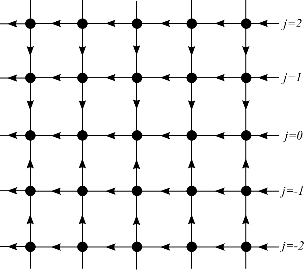
In the context of our present work, we find that the associated graph is composed of directed edges connecting to , along with directed edges connecting to when and to when , all with identical weights of . Furthermore, the associated symmetric graph then has an edge set for which every is connected to and , with identical weights of . Figure 2 provides a visualization of this directed graph. Importantly, one may follow the methods of [2, Section 6] to see that this associated symmetric graph indeed satisfies , PI, and VG(2). Then, the associated symmetric graph leads to expected decay bounds of the order for all . But we note that the only requirement that fails to apply Theorem 4.1 is the condition that , required by Hypothesis 2.
Now, let us take the initial condition given by
It is a straightforward argument to find that with this initial condition we have for all and . The reason for this is that each element with index depends only on those elements to the left of them, and since only the site is activated with this initial condition, it can only influence those elements with to the right of it.
We begin by observing that at index we have
since for all and . Then, moving to index we can substitute the solution for to obtain
since . Continuing in this way, an inductive argument shows that
| (5.2) |
for all . We plot the first few of these functions of visual reference in Figure 3.

Then, for each , differentiating with respect to gives
Hence, attains its global maximum at , and this maximum is given by
Using Stirling’s Approximation we find that . Hence, we see that the solution to the differential equation (5.1) is such that
which shows that there cannot exists a constant such that for all since cannot be bounded uniformly by a constant multiple of the function for all . Therefore, system (5.1) provides an example of a system for which the failure to have Hypothesis 2, but all other hypotheses of Theorem 4.1 hold, leads to solutions which can only decay at a rate of , significantly slower than the that holds for the given associated symmetric graph. This presents a major problem in the analysis of the following section, since we require decays rates of at least to apply bootstrapping arguments to extend from linear ordinary differential equations to local asymptotical stability of nonlinear ordinary differential equation. Hence, in this case an understanding of the associated symmetric graph cannot inform our understanding of the directed graph and the decay of solutions to the differential equation (5.1).
6 Application to Coupled Oscillators
We now reserve this final section for an application of the results of Theorem 4.1. To begin, it is well-known that systems of weakly coupled oscillators can be reduced through a process of averaging to a single phase variable under minor technical assumptions [5, 9, 16, 20]. In complete generality for a countable index set these systems take the form
| (6.1) |
where the function is assumed to be smooth and -periodic in the first variable. The constants are taken to represent intrinsic differences in the oscillators and/or external inputs. In the work of [2] it was assumed that the functions were independent of , leading to the limited focus on identically coupled oscillators. With the results of the previous section, we are now able to expand to more general functions , thus providing a more robust result to that of [2].
A solution to (6.1) is called phase-locked (or synchronous) if it takes the form
| (6.2) |
where are time-independent phase-lags and the elements are moving with identical velocity . Assuming the existence of a phase-locked solution to (6.1) of the form (6.2), the resulting linearization about this solutions leads to the linear operator, denoted , acting on the real sequences by
| (6.3) |
for all , where the prime notation denotes differentiation with respect to the first component of . The form of given in (6.3) should be immediately recognized as of the form of a graph Laplacian operator with
for all . This leads to the nontrivial extension of [2, Theorem 4.5].
Theorem 6.1.
Consider the system (6.1) for a twice-differentiable function such that the derivatives with respect to the first component are uniformly bounded in , and assume this system of equations possesses a phase-locked solution of the form (6.2), denoted . Then, if the resulting linear operator defined in (6.3) satisfies the hypotheses of Theorem 4.1, we have the following: there exists an for which every with the property that
| (6.4) |
leads to a unique solution of (6.1), for all , satisfying the following properties:
- 1.
.
- 2.
for all .
- 3.
There exists a such that
(6.5) for all and .
Due to the results of Theorem 4.1, the proof of Theorem 6.1 is identical to the proof of [2, Theorem 4.5] and is therefore omitted. Prior to concluding this section, we comment on a simple application of Theorem 6.1 to optimally convey these results. Consider system (6.1) with for all , and
where is an infinite matrix of coupling coefficients. We note that no assumption on the signs of the will be made. A trivial example of a phase-locked solution to such a system of coupled oscillators is obtained by taking and for all . Hence, linearizing about this phase-locked solution results in a linear operator of the form on the right-hand side of (1.1) with
for all . Hence, using Theorem 6.1 we see that the stability of this trivial phase-locked solution can be determined by examining the directed graph induced by the coupling matrix . Moreover, if can be shown to satisfy the graph-theoretic hypotheses of Theorem 4.1, one may use Theorem 6.1 to infer local asymptotic stability of the trivial phase-locked solution with respect to perturbations in .
In particular, one can simply define the infinite matrices and by
where is the formal transpose of the infinite matrix . The entries of are exactly the weights of the associated symmetric graph, and hence to satisfy Hypothesis 1 one must first check that the elements of are both nonnegative and uniformly bounded above. Furthermore, it must be so that each row and column contains only finitely many nonzero entries, which this number of nonzero entries is uniformly bounded above over all rows and columns. Checking that the symmetric graph defined by satisfies , PI, and VG(d) for can be followed as in [2, Section 6]. Finally, to satisfy Hypothesis 2 we must have that the norm of the entries of is finite.
Acknowledgements
This work is supported by an NSERC PDF held at Brown University.
References
- [1] M. Barlow, T. Coulhon and A. Grigor’yan. Manifolds and graphs with slow heat kernel decay, Invent. Math. 144, (2001) 609-649.
- [2] J. Bramburger. Stability of infinite systems of coupled oscillators via random walks on weighted graphs, T. Am. Math. Soc., at press.
- [3] I.-L. Chern and T.-P. Liu. Convergence to diffusion waves of solutions for viscous conservation laws, Comm. Math. Phys. 110, (1987) 503-517.
- [4] Y. Chen, S. Z. Khong, and T. T. Georgiou. On the definiteness of graph Laplacians with negative weights: Geometrical and passivity-based approaches, 2016 American Control Conference (ACC), (2016) 2488-2493.
- [5] F. Corinto, M. Bonnin and M. Gilli. Weakly connected oscillatory network models for associative and dynamic memories, Int. J. Bifurcat. Chaos 17, (2007) 4365-4379.
- [6] T. Coulhon and L. Saloff-Coste. Isopérimétrie sure les groupes et les variétés, Rev. Mat. Iberoam. 9, (1993) 293-314.
- [7] T. Delmotte. Parabolic Harnack inequality and estimates of Markov chains on graphs, Rev. Mat. Iberoam. 15, (1999) 181-232.
- [8] G. B. Ermentrout. Stable periodic solutions to discrete and continuum arrays of weakly coupled nonlinear oscillators, SIAM J. Appl. Math. 52, (1992) 1665-1687.
- [9] G. B. Ermentrout and N. Kopell. Multiple pulse interactions and averaging in systems of coupled neural oscillators, J. Math. Biol. 29, (1991) 195-217.
- [10] M. Folz. Gaussian upper bounds for heat kernels of continuous time simple random walks, Electron. J. Probab. 16, (2011) 1693-1722.
- [11] R. Frank and H. Kovarik. Heat kernels of metric trees and applications, SIAM J. Math. Anal. 45, (2013) 1027-1046.
- [12] A. Grigor’yan. Heat kernels on manifolds, graphs and fractals, Prog. Math. 201, (2001) 393-406.
- [13] A. Grigor’yan and A. Telcs. Sub-Gaussian estimates of heat kernels on infinite graphs, Duke Math. J. 109, (2001) 451-510.
- [14] P. Gyrya and L. Saloff-Coste. Neumann and Dirichlet heat kernels in inner uniform domains, Astérisque 33, Soc. Math., France, (2011).
- [15] A. Hoffman, H. J. Hupkes, and E. S. Van Vleck. Multi-dimensional stability of waves travelling through rectangular lattices in rational directions, T. Am. Math. Soc. 367, (2015) 8757-8808.
- [16] F. C. Hoppensteadt and E. M. Izhikevich. Weakly connected neural networks, Springer-Verlag, New York, (1997).
- [17] P. Horn, Y. Lin, S. Liu, S-T. Yau. Volume doubling, Poincaré inequality and Gaussian heat kernel estimate for nonnegative curvature graphs, ArXiv:1411.5087.
- [18] M. Keller and D. Lenz. Unbounded Laplacians on graphs: basic spectral properties and the heat equation, Math. Model. Nat. Phenom 5, (2010) 198-224.
- [19] A. Telcs. The art of random walks, Springer-Verlag, Berlin, (2006).
- [20] L. C. Udeigwe and G. B. Ermentrout. Waves and patterns on regular graphs, SIAM J. Appl. Dyn. Syst. 14, (2015) 1102-1129.
- [21] N. T. Varopoulus. Hardy-Littlewood theory for semigroups, J. Funct. Anal. 83, (1985) 240-260.
- [22] A. Weber. Analysis of physical Laplacian and the heat flow on a locally finite graph, J. Math. Anal. Appl. 370, (2010) 146-158.