Sparse Regular Expression Matching
Abstract
A regular expression specifies a set of strings formed by single characters combined with concatenation, union, and Kleene star operators. Given a regular expression and a string , the regular expression matching problem is to decide if matches any of the strings specified by . Regular expressions are a fundamental concept in formal languages and regular expression matching is a basic primitive for searching and processing data. A standard textbook solution [Thompson, CACM 1968] constructs and simulates a nondeterministic finite automaton, leading to an time algorithm, where is the length of and is the length of . Despite considerable research efforts only polylogarithmic improvements of this bound are known. Recently, conditional lower bounds provided evidence for this lack of progress when Backurs and Indyk [FOCS 2016] proved that, assuming the strong exponential time hypothesis (SETH), regular expression matching cannot be solved in , for any constant . Hence, the complexity of regular expression matching is essentially settled in terms of and .
In this paper, we take a new approach and introduce a density parameter, , that captures the amount of nondeterminism in the NFA simulation on . The density is at most but can be significantly smaller. Our main result is a new algorithm that solves regular expression matching in
time.
This essentially replaces with in the complexity of regular expression matching. We complement our upper bound by a matching conditional lower bound that proves that we cannot solve regular expression matching in time for any constant assuming SETH.
The key technical contribution in the result is a new linear space representation of the classic position automaton that supports fast state-set transition computation in near-linear time in the size of the input and output state sets. To achieve this, we develop several new insights and techniques of independent interest, including new structural properties of the parse trees of regular expressions, a decomposition of state-set transitions based on parse trees, and a fast batched predecessor data structure.
1 Introduction
A regular expression specifies a set of strings formed by characters from an alphabet combined with concatenation (), union (), and Kleene star (∗) operators. For instance, describes the set of strings of s and s such that every is followed by an . Given a regular expression and string , the regular expression matching is to decide if matches any of the strings specified by . Regular expressions are a fundamental concept in formal language theory introduced by Kleene in the 1950’ties [48] and regular expression matching is a basic tool in computer science for searching and processing text. Standard tools such as grep and sed provide direct support for regular expression matching in files, and the scripting language perl [72] is a full programming language designed to support regular expression matching easily. Regular expression matching appears in many large-scale data processing applications such as internet traffic analysis [44, 78, 49], data mining [31], data bases [52, 60], computational biology [63], and human-computer interaction [47].
A classic textbook algorithm for regular expression matching, due to Thompson [70] from 1968, constructs and simulates a nondeterministic finite automaton (NFA) in time, where is the length of and is the number of character symbols in . The simulation processes from left to right and computes a sequence of sets of states such that is the set of states in to which there is a path from the initial state that matches . In 1985 Galil [29] asked if a faster algorithm could be obtained. A sequence of results [62, 11, 10, 12] improved the bound using tabulation or word-level parallelism leading to solutions using either [12] or time [10] time, where is the word length. Finally, Bille and Thorup [13] gave an algorithm using time, where is the number of strings appearing in the regular expression (see also [26, 8]).
The above solutions are based on the classic NFA simulation algorithm from Thompson’s original algorithm [70] and thus achieve the same time with some polylogarithmic factors shaved. Recently, conditional lower bounds have provided evidence for the lack of more significant progress. First, Backurs and Indyk [7] showed in 2016 that we cannot solve regular expression matching in time , for , assuming the strong exponential time hypothesis (SETH) [43]. Then, in 2018 Abboud and Bringmann [1] showed that we cannot solve the problem in time , for , assuming the Formula SAT hypothesis [1]. These results, together with Bringmann, Larsen, and Grønlund [15] and Schepper [67], also studied subclasses of regular expression matching depending on the structure of the operators in the expression, leading to a classification of the complexity of each such subclass. In summary, the complexity of regular expression matching is essentially settled in terms of and .
In this paper, we take a new approach and introduce a density parameter, , that captures the amount of nondeterminism in the NFA simulation on . The density is at most but can be significantly smaller. Our main result is a new algorithm that solves regular expression matching in
time. This essentially replaces with in the complexity of regular expression matching. We complement our upper bound by a conditional lower bound that proves that we cannot solve regular expression matching in time for any constant assuming SETH.
1.1 Sparse Regular Expression Matching
Recall that the NFA simulation algorithm constructs a sequence of state sets such that is the set of states in the automaton to which there is a path from the initial state that matches . The goal of this paper is to explore the complexity of regular expression matching if these sets are sparse. More precisely, let be an instance of the regular expression matching and let be a finite automaton that accepts the set of strings defined by , and let be the sequence of sets of states in the simulation of on . We define the density of wrt. to be
i.e., the density is the total size of the state sets in the simulation of on .
We will focus on density wrt. to the classic position automaton (also known as Glushkov’s automaton), denoted , proposed by Glushkov in 1960 [35, 34] and independently by McNaughton and Yamada [57]. For most NFA constructions [33, 4, 17, 70] (including several textbook constructions [3, 2, 24, 51, 56, 69, 77]), the density wrt. to is a lower bound on the density wrt. to the other NFA construction. The key observation is that the set of states in naturally corresponds to a subset of the set of states in the other constructions. For instance, we can convert Thompson’s NFA, , into the corresponding position automaton, , by carefully contracting -transitions [33, 4, 17]. This implies and thus if an algorithm is efficient in terms of the same algorithm is also efficient in terms of . Hence, for the rest of the paper, we define the density, denoted , to be , and when and are clear from the context we simply write .
Intuitively, the density captures the amount of nondeterminism in the simulation of . At one extreme when all of the state sets are singletons (assuming matches ) and at the other extreme when all of the state sets, except the special , consists of all states. The density can be significantly smaller than in important practical scenarios. For instance, in internet traffic analysis a stream is matched against a large set of rules specified as a regular expression. Typically, most of these packets will only match a small subset of the rules implying a small density of the problem instance.
A related concept is deterministic regular expressions (also known as -unambiguous regular expressions). These are defined as regular expressions for which is deterministic, that is, all state-set transitions on any singleton state set result in a singleton state set. Deterministic regular expressions are widely used in schema languages [19, 14, 30, 61] and have been extensively studied in complexity and automata theory [19, 18, 36, 65, 55, 23, 54]. Groz and Maneth [36] showed how to solve the deterministic regular expression matching problem in time. Note that if the regular expression is deterministic we always have that .
1.2 Sparse State-Set Transitions
Given a set of of states and a character a state-set transition, denoted , is the set of states reachable from via paths of transitions in the NFA that match (for -free NFAs the paths are always single transitions). We can implement the NFA simulation using state-set transitions by setting to be the initial state, and computing for . In our scenario, we are interested in a compact representation of that supports fast sparse state-set transitions, i.e., a state-set computation that is efficient in terms of the sizes of the input set and the output set . Since is the total size of state sets in the simulation this implies an efficient algorithm for sparse regular expression matching.
Surprisingly, few results are known for this problem. If we store explicitly we can compute by computing the union of the endpoints of transitions out of states in labeled . This leads to a data structure that uses space and supports state-set transitions in time. Note that since endpoints of the transition may overlap (see Figure 1(a)) we may need to explore transitions in general. A similar worst-case trade-off also holds for the many variants of the position automaton, see e.g. [20, 42, 5, 59]. While -free NFAs with fewer transitions are known [40, 37, 32, 68] these do not appear to translate to simulations for nor do they improve the above time bound.
Alternatively, we can store Thompson’s automaton, , and use the mapping of states mentioned above to convert state-set transitions on to state-set transitions on . Since is not an -free automaton we can compute a state-set transition using a breadth-first search to explore all paths from that match . This uses space and time. However, it is easy to see that with this approach we may need to traverse large subgraphs of transitions labeled even if the sets or are sparse. Indeed, the efficient solutions in terms of and are based on improving state-set transitions in for the dense case by polylogarithmic factors.
1.3 Results
Our main result is an efficient algorithm for sparse regular expression matching.
Theorem 1.
Given a regular expression with positions and a string of length , we can solve the regular expression matching problem in space and time
Since the density is at most , this essentially replaces with in the complexity of regular expression matching. As an immediate Corollary of Theorem 1 we obtain a solution to deterministic regular expression matching using time and space, thus matching the best known bound of Groz and Maneth [36]. We complement Theorem 1 with an essentially matching conditional lower bound.
Theorem 2.
For any , for any constant , there exists no time algorithm for regular expression matching for any constant assuming SETH.
Theorem 1 is based on a compact representation of the position automaton that supports efficient sparse state-set transitions.
Theorem 3.
Given a regular expression with positions, we can represent the position automaton in space and preprocessing time, such that given any set of states in sorted order and a character , we can compute the state-set transition in time
The output of the state-set transition is also reported in sorted order.
The sorted order of and in Theorem 3 refers to the ordering of the corresponding positions in from left to right (without this condition the factor becomes ). Theorem 3 significantly improves the previous and time bounds. Since any solution must use at least to read the input and write the output the bound is almost optimal.
1.4 Techniques
We develop several new insights and techniques of independent interest, including new structural properties of the parse trees of regular expressions, a novel decomposition of state-set transitions based on parse trees, and a fast batched predecessor data structure.
We show how to decompose any state-set transition into a set of internal transitions on a set of transition nodes of the parse tree of . We have two types of internal transitions: one for and one for . Intuitively, if then the internal -transition of wrt. are all the states/positions in reachable from a state/position in using a transition labeled . The internal -transitions are more complicated to describe, but both types of internal transitions are independent of the state set . We show how to represent in linear space to efficiently compute internal transitions for any node and character .
We identify the set of transition nodes for by first computing a compact representation of a transition tree, which encodes all paths in containing transition nodes in space. Then, we find the set of transition nodes using this tree. The key challenge is that even though the representation of the transition tree is small the tree itself can be significantly larger and contain many nodes that are irrelevant for the character and/or irrelevant for the state set . Using the structural properties of the parse tree we show how to overcome the challenges and efficiently find the set of transition nodes for any and . Computing the internal transitions of all transition nodes could take too long, as the output of these overlap and we could end up using time. However, we prove that these output sets form a laminar family and show how to divide the computations of the internal transitions into computations on a bounded number of non-overlapping intervals.
In combination, the above techniques lead to an space representation of that supports state-set transitions in time. The bottleneck here is computing a predecessor queries in time. We present a simple two-level data structure that solves this batched predecessor problem in time while maintaining linear space leading to our final structure. Using this solution for sparse-set transitions to implement the NFA simulation implies our main result for sparse regular expression matching of Theorem 1.
The lower bound follows from a reduction from the orthogonal vectors problem (OVP). We prove that given , for any constant , we can construct an instance of regular expression matching such that the existence an algorithm for regular expression matching violates SETH. The reduction is based on the reduction by Backurs and Indyk [7] and is a fairly straightforward generalization of their lower bound.
1.5 Related Work
Another NFA construction, by Chang and Paige [21], considered compact representations of that support efficiently implementing NFA to DFA conversion by subset construction. They presented a linear space representation that supports efficiently computing the set of states reachable via any character from a state-set in time . Since can be much larger than this does not imply an efficient sparse state-set transition.
Some measures of nondeterminism of NFAs have been studied in automata theory, e.g., width, ambiguity, string tree width, string path width, and cycle height [46, 50, 53, 39, 45]. These focus on the complexity of computing measures of the nondeterminism of a given NFA. In contrast, we study the complexity of regular expression matching in terms of the nondeterminism of a simulation on a given NFA and input string.
As mentioned, Bille and Thorup [13] considered the number of strings in the regular expression as a parameter for regular expression matching. They gave an algorithm using time. It is straightforward to construct instances of regular expression matching (for a matching regular expression) such that either and or and hence this result is incomparable to ours. Cotumaccio, D’Agostino, Policriti, and Prezza [22] studied the indexing version of regular expressions, where the goal is to preprocess a regular expression in order to allow for fast matching given a query string. They considered the co-lexicographic width of an automaton. Applying their construction in the matching setting gives an algorithm that runs in , where is the width of the co-lexicographic order and comes from the preprocessing of the automaton.
Several papers have studied the related problem of string matching in labeled graphs. For example, Rizzo, Tomescu, and Policriti [66] studied the problem of matching a pattern on a labeled graph parameterized wrt the size of the labeled direct product graph, and Nellore, Nguyen, and Thompson [64] studied string matching in graphs parameterized by the size of the powerset automaton.
1.6 Outline
We review regular expressions and automata in Section 2 and the parse tree view of regular expressions in Section 3. We introduce internal transitions, state-set decompositions, and transition trees in Section 4 and present our main algorithm for sparse state-set transitions in Section 5. In Section 6, we present the improved batched predecessor data structure. We use this to obtain the final result for sparse state-set transitions of Theorem 3 which we then use to obtain Theorem 1. Finally, we show the lower bound of Theorem 2 in Section 7.
2 Regular Expressions and Automata
We briefly review the classical concepts used in the paper. For more details, see, e.g., Aho et al. [2].
Regular Expressions
We consider the set of non-empty regular expressions over an alphabet , defined recursively as follows. If then is a regular expression, and if and are regular expressions then so is the concatenation, , the union, , and the star, . We often omit the concatenation when writing regular expressions. The language generated by a regular expression is defined as follows. If , then is the set containing the single string . If and are regular expressions, then , that is, any string formed by the concatenation of a string in with a string in , , and , where and , for .
Finite Automata
A finite automaton is a tuple , where is a set of nodes called states, is a set of directed edges between states called transitions each labeled by a character from , is a set of start states, and is a set accepting states. In short, is an edge-labeled directed graph with designated subsets of start and accepting nodes. is a deterministic finite automaton (DFA) if does not contain any -transitions, all outgoing transitions of any state have different labels, and there is exactly one start state. Otherwise, is a nondeterministic finite automaton (NFA).
Given a string and a path in we say that and match if the concatenation of the labels on the transitions in is . Given a state in and a character we define the state-set transition to be the set of states reachable from through paths matching (note that the paths may include transitions labeled ). For a set of states we define . We say that accepts a string if there is a path from a state in to a state in that matches . Otherwise, rejects . We can use a sequence of state-set transitions to test acceptance of a string of length by computing a sequence of state-sets , given by and , . We have that iff accepts .
The Position Automaton
Given a regular expression , we can construct an NFA accepting precisely the strings in by several classic methods [57, 34, 70]. In particular, Glushkov gave an important construction called the position automaton or Glushkov automaton. The position automaton is an -free NFA consisting of only states and transitions (See Figure 1). Each state except the start state corresponds to a position. Intuitively, each state-set in a state-set simulation is the set of positions in that correspond to a match of a prefix of .
We review the details of the position automaton in the following. Let be a regular expression with character symbols from an alphabet . The position of a character in is the index of the character in the left-to-right order among the characters in . The set of positions in , denoted , is the set . The label of a position , denoted , is the character at position . The subset of positions labeled is denoted . When is clear from the context we abbreviate to phb .
The marked regular expression of , denoted , is obtained from by subscripting each character in with its position. Similarly, the marked alphabet, denoted , is obtained from by adding subscripts. The marked regular expression defines the language over the marked alphabet . Note that . Given a position we define to be the label of in . The and set of represent the positions that match the first and last character, respectively, in some string in . Given a position , the set of and is the set of positions that can follow a position in . More precisely,
We then define the position automaton for as the NFA , where
3 Regular Expressions as Trees
Throughout the rest of the paper, let be a regular expression with positions and let denote the state-set transition function of the position automaton for . For simplicity in the presentation, we will focus on implementing on the positions of and ignore the extra start state of the position automaton. The extra start state is straightforward to represent with additional linear space and is only needed in the initial step of state-set simulations.
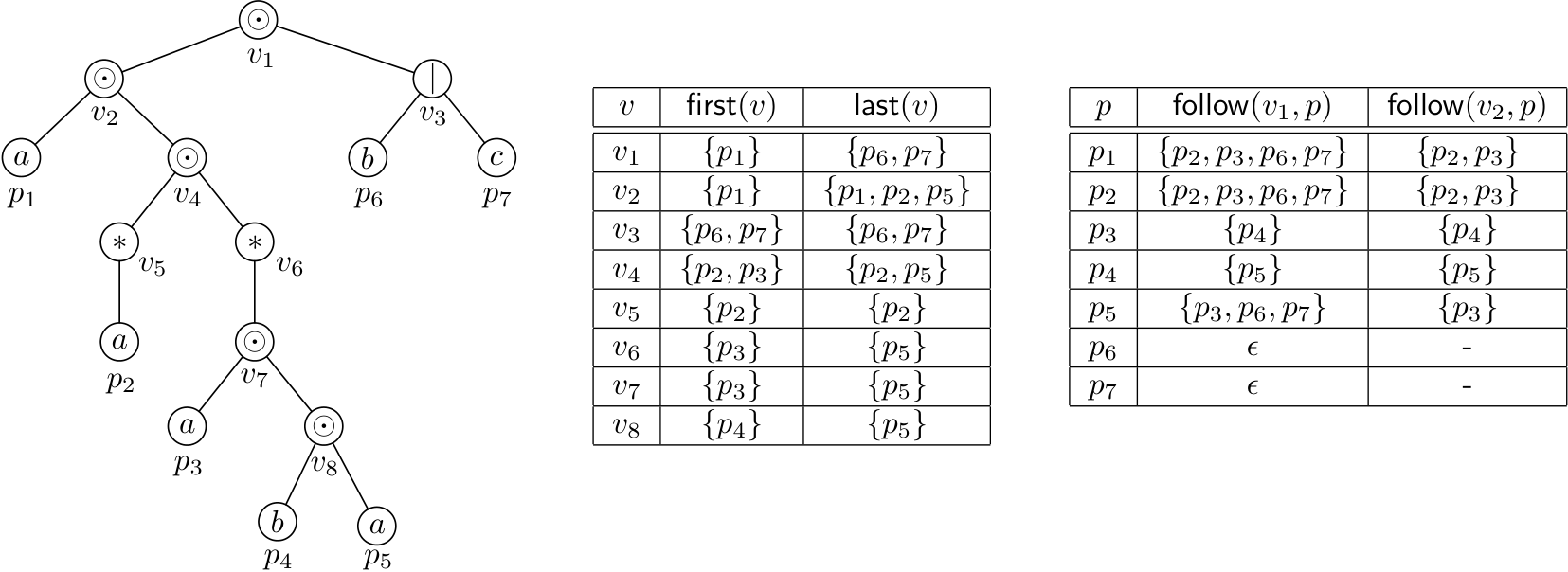
We identify regular expressions by their parse trees (see Figure 2). Note that the leaves in left-to-right order are the positions. We call the three types of internal nodes -nodes, -nodes, and -nodes. For a -node or -node the left and right child are denoted and , respectively, and for a -node the single child is denoted . The depth of a node in is the number of edges on the path from the root of to . We denote the subtree (equivalently subexpression) rooted at a node by . If then is an ancestor of , denoted , and if and then is a proper ancestor of , denoted . If is a (proper) ancestor of then is a (proper) descendant of . A node is a common ancestor of and if it is an ancestor of both and . The lowest common ancestor of and , , is the common ancestor of and of greatest depth. The lowest star ancestor of a node , denoted , is the lowest ancestor of that is a -node.
We extend the definition of labels to internal nodes. For each internal node , the label of , denoted , is a set of characters such that iff for some positions and both labeled . In Figure 2, since and . Since the total number of internal nodes containing label is the total size of all labels is . For a node we extend our notation to define , , , and to denote the sets on the subexpression (see Figure 2).
In our setting, we will often view the and sets from the perspective of a single position and consider the nodes for which appears in the corresponding and sets, respectively. Specifically, we define the first extent and last extent of a position , respectively, to be the set of nodes in given by and . Furthermore, for a set of positions , we write and . For instance, in Figure 2 we have . We define the first extent and last extent of an internal node , to be the sets and , respectively.
The first sets and the last sets, respectively, form a laminar family. That is, for any two nodes in the parse tree, their first sets, respectively, last sets, are either disjoint or one is contained in the other. That implies that the set of nodes in , respectively, , forms a path from position to an ancestor of .
Lemma 4.
Let be a position in a regular expression and let and be nodes in such that . If , then and if , then .
Proof.
We have that is a subexpression of and is a position in . Then, if then . Similarly, if then . ∎
4 Internal Transitions, State-Set Decompositions, and Transition Trees
We now introduce the main structural properties of state-set transitions that we need for our fast sparse state-set transition algorithm in Section 5. We first characterize state-set transitions in the position automaton in terms of and using the following important property.
Lemma 5.
Let and and . Then, iff either
- (i)
is a -node, , and , or
- (ii)
.
Lemma 5 has appeared in various forms in earlier work [36, 21, 65]. For our purposes, we state it in terms of lowest common ancestors and first extents and last extents. Lemma 5 states that a position can only appear in through a -node or a -node. We write if (i) is satisfied and if (ii) is satisfied.
4.1 Internal Transitions
Given an internal node , an internal transition on and a character will correspond to the conditions on and in Lemma 5 while ignoring the condition on . In general, we will also specify a range of positions we are interested in. Formally, given an internal node , a character , and positions and , define the internal -transition and internal -transition, denoted and , respectively, as follows.
When the range includes all positions we drop the subscript, that is, and . For instance, in Figure 2 we have , , and .
4.2 Transition Nodes
Given a state-set transition , the transitions nodes are a set of nodes such that if we compute the union of internal transitions on we obtain . Formally, we define the -transition nodes and -transition nodes of , denoted and , respectively, as
In combination, the set of transition nodes is the union of the -transition nodes and the -transition nodes.
Lemma 6.
For any set of positions and a character ,
| (1) |
Proof.
Let denote the right handside of (1).
We first show that . Let and be positions with such that . Then, and hence , , and satisfies either case (i) or (ii) in Lemma 5. If (i) is satisfied, is a -node and and . By definition, , and thus . Similarly, if (ii) is satisfied, then , and it follows . This implies that .
To show first suppose . Then, and there is a -node such that and , which implies that for some . By Lemma 5(i) . If then there exists a such that and . It follows from the definition of and By Lemma 5(ii) that there exists a and a such that and . Since both and are descendants of we have that is a (not necessarily proper) descendant of . It follows from Lemma 4 that and . Thus by Lemma 5(ii) we have . ∎
We show that the total size of the two sets and is ).
Lemma 7.
We have and .
Proof.
By definition every node in is the lowest common ancestor of some position and some position . The number of distinct pairwise lowest common ancestors of a subset of leaves in a tree cannot exceed . Therefore, the number of lowest common ancestors between positions in and positions in can never be larger than . The same argument holds for the number of nodes in . ∎

The internal transitions on the set of transition nodes are not disjoint and hence we cannot afford to compute internal transitions on each of the transition nodes explicitly. Fortunately, by Lemma 4, the internal -transitions (resp. -transitions) of the nodes from (resp. ) form a laminar family. We use this to divide the computations of the internal transitions into computations on a bounded number of non-overlapping intervals. We implement this idea by compactly encoding all relevant transition nodes in the transition tree defined in the following.
4.3 Transition Trees
Let be a set of positions. Given a state-set transition , we define the transition tree as the subtree of induced by all nodes in and their ancestors (see Figure 4(a)). A segment in is a path from a leaf or a branching node to (but not including) the nearest branching node above it (or to the root if no such branching node exists). The root node is its own segment (see Figure 4(b)). The bottom node of a segment is denoted . Note that is always a branching node, a leaf, or the root. Any branching node in is the lowest common ancestor of two nodes in and vice versa. Hence, we can compactly store in space by storing and the branching nodes with pointers into .
The following observation follows immediately from the fact that all nodes in and their ancestors are contained in .
Observation 8.
Let be the transition tree for in . If is a transition node for then is a node on a segment in .
Thus it is enough to consider the nodes in the transition tree when computing the set of transition nodes.
Observation 9.
Any -node that is an internal node on a segment and where must have its left child on the same segment.
To see why, observe that since , then is an ancestor of a node in , and thus by definition of , belongs to . Since is an internal node on a segment , only one of its children belongs to . Therefore, must also belong to segment .
We will show in Section 5.2 that the transition tree and the key information we need in our algorithm can be computed in time.
5 Sparse State-Set Transitions
We now present our space data structure that supports computing a state-set transition in time. We describe the data structure and analyze the space and preprocessing time in Section 5.1. The high-level idea of our sparse state-set algorithm is to identify the transition nodes for and using the transition tree. The state-set transitions for each set of nodes induce a partition of into nested intervals. We partition these intervals into non-overlapping intervals and then compute the internal transitions for each new interval. We then compute the union of these, which by the decomposition in Lemma 6, is precisely the set . We describe how to construct the transition tree in Section 5.2. In Section 5.3 we describe how to find the set transition nodes and how to construct the intervals. In Section 5.4 we we show how to compute the internal transitions efficiently. Finally, in Section 5.5 we put everything together to get an algorithm for computing a state-set transition in time.
5.1 Data Structure
We store the regular expression with labels on leaves and internal nodes together with the following components.
- •
For each node in , we store the range of positions that are descendants of , the depth of , the highest node in , and the highest node in . We also store a pointer to the lowest ancestor of such that is an -node and , and a pointer to its lowest star ancestor.
- •
At each branching node we store the position of the rightmost leaf in and the position of the leftmost leaf in .
- •
Data structures for that supports lowest common ancestor queries and first label queries. Given a node and a character , a first label query, denoted , returns the lowest ancestor of whose label contains .
Furthermore, we store the following information for each .
- •
Arrays and , where is the th position labeled in the left-to-right ordering of , and is the depth of the highest node in .
- •
A data structure supporting predecessor and successor queries on the positions in . That is, given any position in the predecessor (successor) query returns the position in of the nearest position labeled to the left (right) of including itself. For a branching node , we define the successor of in as the successor in of the leftmost leaf in . Note that this corresponds to the first position labeled after in the order obtained by an inorder traversal of the nodes in . Similarly, we define the predecessor of in as the predecessor in of the rightmost leaf in .
- •
A data structure on that supports range minimum queries. Given any pair of indices and , the range minimum query on returns a minimum value in the subarray .
- •
For each node containing label :
- –
A pointer to the lowest proper ancestor of such that , , and is non-empty. If no such exists we store a null pointer to indicate this.
- –
A pointer to the lowest proper ancestor of labeled such that there exists a where if and if . If no such exists we store a null pointer to indicate this.
- –
The range of positions in that are descendants of , of , and of , respectively.
- –
The idea of the -pointers is that they form a chain of prospective nodes for with label . Any node from with label on a segment has its left child on the path and , so it is included in this chain. We show that at most one node can be from on each segment that does not have label . Furthermore, given a segment , the nodes from the chain on that belong to form a subchain starting from the lowest node of the chain that is on to (not including) the first node in the chain that is either not in or not on . Similarly, the -pointers form a chain of prospective nodes for with label .
Space
The regular expression and the labels use space. The arrays and , , use space in total. We use linear space and linear preprocessing time data structures to support lowest common ancestors in constant time [38, 9], first label queries in time [25], predecessor queries in time [75, 58], and range minimum queries in constant time [38, 9]. For each alphabet character, the total size of these data structures is linear in the number of leaves labeled with that character. Thus in total the space for these data structures is linear in . The cited data structures for predecessor queries both use randomization, but since we only need a static structure it is straightforward and well-known how to obtain the same bound deterministically by combining deterministic dictionaries [37] with a simple two-level approach (see, e.g., Thorup [71]). We store at most two pointers for each label in and a single pointer for each position using space. The remaining information uses space.
Preprocessing
We compute the range of positions that are descendants of , the depth of , the and pointers, and the positions of and using tree traversal in linear time. To compute the highest node for each node in , we first compute for each node if using a linear time bottom-up tree traversal. In top-down traversal we then compute the highest node in for each node using the following rules: If is the left child of an -node and then . Otherwise, . We compute the highest node in similarly. We construct the arrays and , for all in a single tree traversal.
To compute the remaining information we do the following for each . Construct a tree containing all nodes with label . To do this, we use queries on each consecutive pair of leaves in from left to right. By keeping track of the depths of the nodes and checking if the newest node is an ancestor of the previous node it is straightforward to implement this in linear time. To compute the -pointers we do a top-down traversal of . In each node we check if and are empty using range minimum queries on . To check if we do the range minimum query on the range of positions in in . If the depth returned is less than or equal to then is non-empty. For we do the query separately on the intervals corresponding to the left and the right child and we compare with the depth of . With this information, we can compute the -pointers during the traversal of in constant time per node. The total size of all the trees , since each tree has size . Thus the total time used for each is . Hence, it follows that the total preprocessing time is .
5.2 Constructing the Transition Tree
We say that a node is a -live node if and is a -node. Note that any node in is a -live node and a node in the transition tree . It follows from Observation 9 that any -live node that is an internal node on a segment has its left child on the segment. A segment in is called a -segment if is not the root and .
We compute the compact representation of the transition tree as follows. Let be the set of leaves and repeatedly take the of adjacent nodes to form the internal nodes and the segments of . Using a tree traversal on the compact transition tree we also compute for all branching nodes in the depth of the highest node in , all -live branching nodes in , and all -segments of . Hence, we have the following result.
Lemma 10.
In time we can compute the transition tree of , for all branching nodes in the depth of the highest node in , all -live branching nodes in , and all -segments of .
Observation 11.
We can check in constant time if a node is in given the segment it is on.
If is a leaf or a branching node, we already computed the information. Otherwise, is an internal node on a segment . Then we compare the depth of with the depth of the highest node in . Now is in if and only if the depth of is at least .
5.3 Computing Transitions Nodes and Intervals
We construct two sets of nodes and that consists of all nodes in and , respectively, together with a constant number of other nodes per segment. We compute these sets for each segment using a depth-first traversal of the transition tree. We also construct sets and , that partition into intervals in order to avoid recomputing overlapping internal transitions. We associate each interval with the lowest node from (respectively ) that can contain the positions in its internal transition (see Figure 5).

5.3.1 Computing Transitions Nodes
We first explain how to compute the transition nodes using the -pointers and the transition tree.
Computing
We find for each segment all -transition nodes for as follows.
- 1.
Find first relevant -node on : Set . If is not on or is not an -live node stop.
- 2.
Find first -transition node on : Compute the successor of in , i.e., is the successor in of the leftmost leaf in . If no such exists stop, otherwise set . If is not on stop. If is a -live node not labeled we add to . Now compute . If is not a -live node set .
- 3.
Repeatedly find next transition node by following -pointers: We find all -transition nodes by repeatedly following -pointers from and adding the visited nodes to as follows. As long as and is on we add to and set .
Computing
We find for each segment all -transition nodes for .
- 1.
If is not a -segment we stop.
- 2.
Find first -transition node on : Compute the predecessor and successor of in and let be the lowest of and . If is not on stop. If and we add to .
- 3.
Repeatedly find next transition node by following -pointers: We first compute . We find all -transition nodes by repeatedly following -pointers from and adding the visited nodes to as follows. As long as and is on we add to and set .
Complexity
We first analyze the time used to find . We use time to follow pointers. Additionally, we use time to compute the first label queries, as we do one first label query on each of the segments. The time to check if a node is -live is constant. For all the bottom nodes of the segments the information is stored in the tree and for all the other nodes we can check in constant time if as described in the end of Section 5.2 as will always be on the current segment. Thus the total time used is . Similarly, we use time to compute . Next we analyze the size of and .
Lemma 12.
.
Proof.
We will prove that at most one node from from each segment is not in . Recall that consists of all the -nodes that have and .
Any node added to in step 3 except the first one has , since they were found using -pointers. Thus, . A node is only added if it is -live, i.e., . Thus . Therefore, only the first node found on each segment—the node from step 2—might not be in . Since there are segments in we have . By Lemma 7 we have and thus . ∎
The argument for the size of is similar, but here we show that the number of nodes in that are not in is at most .
Lemma 13.
.
Proof.
We will prove that at most two nodes from from each segment is not in . Recall that consists of all the nodes such that there exists a and a such that and .
Any node added to by following -pointers has and . Furthermore, if is on the segment , then there exists a position and a position . This implies that is in . The argument for the case where is on the segment is symmetric.
At most two other nodes are added to for each segment (the first two nodes are added to on each segment). It follows that the total number of nodes in is at most . By Lemma 7 we have and thus . ∎
Correctness
We argue that the sets and include all transition nodes for . We need the following lemma, which follows from the path structure of the last extent sets.
Lemma 14.
Let be an -live node and let be the segment in containing . All -nodes below on with on are also -live.
Proof.
If is not on then is a branching node in by construction of . Thus and it is trivially true since has no descendants on . We will prove the case on by contradiction. Since is -live there exists a node such that . Furthermore, is an ancestor of some node in . Let . If then . If then is a branching node in . Since there are no branching nodes internally on a segment it follows that . By Lemma 4 all nodes on are in . ∎
We are now ready to prove that is contained in . Let be a node in . There are two main cases in the proof depending on whether labeled or not. If not, then we show that in step 2. If is labeled , then we show, that either is the first -node on the segment, in which case it is added as the first node in step 3, or it is a node on the path induced by the -pointers. As we proved in Lemma 14 above, all the nodes on this path below are also -live and we show by induction that all the -live nodes from on this path are added to in step 3.
Lemma 15.
.
Proof.
Let . By definition is -live, , and . Let be the segment in containing . We want to show that is added to . Define and as the successor of in as in step 1 and 2 of the algorithm. There are two cases depending on whether has label or not.
Case 1: . We first show that . Since is an -node we have that is an ancestor of . If is a proper ancestor of then . Since there is a position such that . This implies that . If then and we are done (see Figure 6(a)). Assume and let . Since we have . But then . Thus and has label which is a contradiction (see Figure 6(b)). It follows that . Thus, since is -live and not labeled , is added to in step 2.
Case 2: . There are two subcases. In the first case . Then in step 1. Since we have in step 2. Since is labeled we have . Since we add to in the first iteration in step 3.
In the other case . Let
Clearly, , and thus follows from the following claim.
Claim 16.
Let be a node in . Then is added to in step 3.
Proof: We prove the claim using induction on the height of . For the base case let be the lowest node in . Since is -live it follows from Lemma 14 that is also -live and thus we continue from step 1 to step 2. Since we have , where as computed in step 2. Now either and then is added to in the first iteration in step 3. Otherwise, . Since is the lowest node in then has its -pointer pointing to . Now either is an -live node, in which case is set to in the end of the first iteration of step 3. Otherwise, is set to in the end of step 2. In either case, is added to in step 3.
Induction step: Let be a node that is not the lowest node in . Let be the highest node in that is a proper descendant of . Then points to . Let . By definition of the -pointers and . Now, since , and , we have . If then contradicting that is the highest descendant of in . Thus . By the induction hypothesis, was added to in step 3, whereafter we follow the -pointer to and add in the next iteration. ∎
We will now prove that . Here is an outline of the proof. Recall that for any node in , there exists a position in and a position in , such that is the of and and is in both and . We first prove that the segment containing is a -segment. Then it follows easily that if then is added to in step 2 or 3. If is not the bottom node on , then due to the properties of the transition tree the child of not on contains in its subtree. We then show that if is not labeled then it is added to in step 2. Otherwise, it is either added as the first node in step 3, or it is a node on the path induced by the -pointers on . By similar arguments as those in the previous proof all nodes below on this path has their -node in , the first node on the path is found by a firstlabel query in step 3, and thus is added to in step 3. See Figure 6.
Lemma 17.
.
Proof.
Let be a node in . Then there exists a position and a position such that and . Let be the segment is on. We first prove that is a -segment: If then and thus is a -segment. Otherwise, . By construction of we have and thus by Lemma 4 , since is an ancestor of .
We now prove that . Let be the lowest of and as computed in step 2. If then and thus . If then is added to in step 2. Otherwise, it is added in step 3.
If , let be the child of that is on and let be the child not on . By construction of we have and , since all bottom nodes of segments in have a position from in their subtree and any node that is the of two nodes in is a branching node in . Thus . There are two cases depending on whether is labeled or not.
Case 1: . Since we have . Thus, either or is in and then . Therefore, is added to in step 2.
Case 2: . Then is the of two positions in , which implies that there exists a position labeled in . It follows that either or is in and thus . If then is added to in the first iteration in step 3. Otherwise, . Let . If then is added to in the first iteration in step 3.
If then . Since and we have . Therefore, the highest proper descendant of labeled has its -pointer pointing to . It follows that there is a chain of -pointers from to . It remains to show that for all the nodes in this chain we have . If this is true we will reach in step 3. Since then all nodes on are ancestors of . Since we have . By Lemma 4 we have . ∎
5.3.2 Computing the Intervals
We now compute the lists and of intervals for the nodes in and , respectively. We do this by processing the nodes and in inorder using a depth-first left-to-right inorder traversal of .
First, we compute for each node in the range of positions labeled that are descendants of . If is labeled the range is stored at and otherwise we use the predecessor data structure to compute it using the range stored at . Similarly, we compute for each node in the range of positions labeled that are descendants of .
Computing
We compute the list of intervals by a depth-first left-to-right inorder traversal of . We maintain a stack keeping track of the deepest node not finished and a counter equal to the left starting point of the currently open interval. If there is no open interval . Initially, and .
For each node in inorder do the following:
- •
When we meet in the traversal after traversing the left subtree of : If append to . Set and push onto the stack .
- •
When we finish the traversal of the subtree containing : Note that in this case . If append to . Pop from . If the stack is now empty set , otherwise set .
Note that might not be in , in which case the two steps for follow immediately after each other.
Computing
We maintain a stack and counter as before.
For each node in inorder do the following:
- •
First time we meet in the traversal: If append to . Set and push onto the stack .
- •
Last time we meet in the traversal: Note that in this case . If append to . Pop from . If the stack is now empty set , otherwise set .
Complexity
To compute the ranges use time as at most one node in on each segment is not labeled . We will store the nodes in in increasing order of depth for each segment. This is easy to maintain as we find them in order of decreasing depth. This way we can do the depth-first left-to-right traversal on the nodes of in in linear time in the size of . Thus computing takes time .
Similarly, we use time to compute . In summary, we have the following lemma.
Lemma 18.
The sets and , and the lists and , can be computed in time .
5.4 Internal Transitions
We will compute and return the state-set transition by computing the internal transitions on the nodes in and . Next, we show how to compute internal transitions efficiently using 3-sided range queries. We assume that the range is given as indexes in .
Computing .
Given an -node , a character , and a range we compute as follows. We perform a 3-sided range reporting query on . That is, we return all positions in with a value less than or equal to . This can be done by a standard technique of recursively applying range minimum queries as follows. Let be the position returned by range minimum query on . If return and recurse on the ranges and . We stop if this is not the case or if the range is empty.
For instance, suppose we compute in our example in Figure 2. The range in corresponds to the positions , , and . We find the highest first extent in to be corresponding to both and . Suppose corresponding to . Then we compare with and since is an ancestor of we report and repeat on the subarrays and . On we return , while on we do not get a position since is a proper descendant of .
Note, that we can get the output in sorted order if we first recurse on the range , then report , and then recurse on the range .
The algorithm returns all positions with label in such that and is thus correct. Each recursive call uses constant time and we repeat at most times. Hence, in total we use time.
Computing .
To compute an internal transition for the -case we do a 3-sided range reporting query . Correctness follows as above and the time and space bounds are the same.
In summary, we have the following result.
Lemma 19.
Let be a regular expression of size . Given we can build a data structure in space and preprocessing time, such that given a node in , a character , and a range we can compute in sorted order in time and in sorted order in time .
5.5 Computing State-Set Transitions
Given a set of positions and a character , we compute the state-set transition as follows. For simplicity, we assume that the positions in are sorted according to their left-to-right order since otherwise we can sort them in additional time using integer sorting. The final algorithm for computing fast state-set transitions is as follows.
- 1.
- 2.
We then compute , , , and as in Subsection 5.3.
- 3.
Finally, we compute and return the state-set transition by computing
by processing and from left-to-right using the procedure from Subsection 5.4 that computes and in sorted order. Since both lists and are sorted the lists and are also sorted. We merge these two lists to get the final output.
Analysis of the algorithm
Step 1 uses time by Lemma 10, and Step 2 uses time by Lemma 18. By Lemma 19 the time to compute all internal transitions in step 3 is
| (2) |
The length of list is as each interval endpoint is due to meeting a node in for the first or last time in the traversal. Similarly, . Hence, (2) is . The time to merge the two lists is linear in the total size of the lists since the lists are sorted. Thus the time for step 3 is . Plugging in the bounds from Lemma 12 and 13 we get a total running time of .
Correctness
We have already proved that and . Thus, by Lemma 6 the set of positions computed in step 4 is . There are at most nodes in . These nodes are all in and thus the set of internal transitions on these will all be in . Similarly, for the nodes in .
It remains to show that the partition into lists is correct. We show that a position is covered by the lowest node in such that , i.e., where covered means that for some such that . This follows easily from the properties of the inorder traversal. The arguments for are similar. For completeness, the full proof is shown below.
Lemma 20.
We have
Proof.
We split the proof into two cases.
Case 1: . We are only adding subranges of the range of for any node in to . This immediately implies that .
For the other direction, let be a position in and let be the deepest node in such that . We will show that for some such that .
Let and . If neither nor are in then nothing happens with and the stack after the step where we add to the top of the stack until we leave the last time. At this point and and is appended to . If then when we leave , node will be on top of the stack and . If also then is the next node from we process in our inorder traversal. When we meet before traversing its right subtree we add to . Since we have . If then the next change we perform is when leaving . Here we add to . If only then we have and when we process the first time (after visiting its left subtree). Then we add to .
Case 2: . The arguments are similar to case 1. We are only adding subranges of the range of for any node in to . This immediately implies that .
For the other direction let be a position in and let be the deepest node in such that . We will show that for some such that .
If there are no other nodes from than in then nothing happens between the first and last time we meet in the traversal and is appended to when we meet the last time. Similarly to case 1, let and . If then when we leave , node will be on top of the stack and . If also then is the next node from we process in our traversal. When we meet the first time we add to . Since we have . If then the next change we perform is when leaving . Here we add to . If only then we have and when we process the first time (after visiting its left subtree). Then we add to . ∎
In summary, we have the following result.
Lemma 21.
Given a regular expression of size , we can build a data structure in space and preprocessing time such that given any set of positions in and character , we can compute in time.
6 Speeding Up State-Set Transitions
We now show how to improve the run time of computing a state-set transition from to while still using linear space. Finally, we show how to use this to obtain the main results of Theorems 1. We now require that the input positions in are sorted and the output positions in are reported in sorted order.
First, observe that the factor is from computing predecessor queries and first label queries in steps 2 and 3 in the main algorithm in Section 5.5. The first label queries in turn are reduced to computing predecessor queries on the Euler tour of [25]. In both cases, we need to answer a batch of predecessor queries on a set of size from a universe of size . The batch is provided in sorted order and the output should also be sorted.
We use a simple two-level data structure as follows. We first partition the universe into intervals of size (except possibly the last which may be smaller). For each interval, we store a predecessor data structure over the subset of the elements in the interval using a reduced universe of size . Furthermore, we also store a pointer to the nearest non-empty smaller interval. Using the same predecessor data structure as in Section 5.5 for each interval the total space is . We answer a batch of predecessor queries according to the following two cases:
- 1.
If we process each predecessor query in the batch by identifying the at most two intervals containing the answer and then querying these predecessor data structures. In total, this uses time.
- 2.
If we simply merge the sorted batch of queries with the input set using time.
Since the batch is sorted we can also return the output in sorted order in time. It follows that the running time is bounded by . Plugging into to the algorithm of Section 5.5, we obtain a data structure that uses space and supports computing a state-set transition in time . This completes the proof of Theorem 3.
Next consider Theorem 1. Let be a string of length and let be the state-sets in the simulation of on . We implement the state-set transitions using Theorem 3. Note that each state-set transition produces the output in sorted order as required. Since logarithms are concave we have that the total time for the state-set transitions is
The algorithm uses space to store the representation of and at most two state sets during the simulation. This completes the proof of Theorem 1.
7 Conditional Lower Bound
We now prove the conditional lower bound of Theorem 2. Our lower bound follows the reduction of Backurs and Indyk [7] from the orthogonal vectors problem (OVP) to regular expression matching.
The orthogonal vectors problems is defined as follows. Given two sets such that , , determine if there exists and such that . For any for some and any constant , any algorithm for OVP with running time violates SETH for [76, 16].
Backurs and Indyk [7] showed hardness of regular expression matching using a reduction from OVP. Given an instance of OVP they show how to construct a regular expression and a string in time such that matches if and only if there exists and such that . The reduction works in time, the lengths of both and is , and the alphabet is . The regular expression has the form
Here is a regular expression of length with the property that a substring of can be derived from if and only if there exists and such that . The precise definition of , , and can be found in [7].
We claim that . To see this first note that is at most . For the lower bound, consider the sequence of state sets in the NFA simulation, and focus on the first positions in , i.e., the positions corresponding to the subexpression immediately before . Since is a string of s and s, we have and . Thus, and hence the claim follows. See Figure 7(a).
We can now prove the following theorem.
Theorem 22.
Given and and a constant , where , we can construct in time a regular expression and a string , such that there exists and where if and only if . The size of and is and .
Proof.
We construct our instance , from and as follows.
where .
Clearly, matches if and only if matches . Furthermore, the NFA simulation on the first characters must produce singleton state sets (see Figure 7(b)). Hence, we have that . Since we have that . ∎
8 Acknowledgments
We thank the anonymous reviewers whose comments and suggestions significantly improved the presentation of the paper.
References
- [1] Amir Abboud and Karl Bringmann. Tighter connections between formula-sat and shaving logs. In Proc. 45th ICALP, 2018.
- [2] Alfred V. Aho, Ravi Sethi, and Jeffrey D. Ullman. Compilers: principles, techniques, and tools. Addison-Wesley Longman Publishing Co., Inc., 1986.
- [3] Alfred V Aho and Jeffrey D Ullman. The theory of parsing, translation, and compiling, volume 1. Prentice-Hall Englewood Cliffs, 1973.
- [4] Cyril Allauzen and Mehryar Mohri. A unified construction of the Glushkov, Follow, and Antimirov automata. In Proc. 36th MFCS, pages 110–121, 2006.
- [5] Valentin M. Antimirov. Partial derivatives of regular expressions and finite automaton constructions. Theor. Comput. Sci., 155(2):291–319, 1996.
- [6] Alberto Apostolico and Concettina Guerra. The longest common subsequence problem revisited. Algorithmica, 2(1-4):315–336, 1987.
- [7] Arturs Backurs and Piotr Indyk. Which regular expression patterns are hard to match? In Proc. 57th FOCS, pages 457–466, 2016.
- [8] Djamal Belazzougui and Mathieu Raffinot. Approximate regular expression matching with multi-strings. In Proc. 18th SPIRE, pages 55–66, 2011.
- [9] Michael A. Bender and Martin Farach-Colton. The LCA problem revisited. In Proc. 4th LATIN, pages 88–94, 2000.
- [10] Philip Bille. New algorithms for regular expression matching. In Proc. of the 33rd ICALP, pages 643–654, 2006.
- [11] Philip Bille and Martin Farach-Colton. Fast and compact regular expression matching. Theor. Comput. Sci., 409(3):486–496, 2008.
- [12] Philip Bille and Mikkel Thorup. Faster regular expression matching. In Proc. 36th ICALP, pages 171–182, 2009.
- [13] Philip Bille and Mikkel Thorup. Regular expression matching with multi-strings and intervals. In Proc. 21st SODA, pages 1297–1308, 2010.
- [14] T Bray, J Paoli, CM Sperberg-McQueen, Y Mailer, and F Yergeau. Extensible markup language (XML) 1.0 5th edition. Technical report, W3C, 2008.
- [15] Karl Bringmann, Allan Grønlund, and Kasper Green Larsen. A dichotomy for regular expression membership testing. In Proc. 58th FOCS, pages 307–318, 2017.
- [16] Karl Bringmann and Marvin Künnemann. Quadratic conditional lower bounds for string problems and dynamic time warping. In 2015 IEEE 56th Annual Symposium on Foundations of Computer Science, pages 79–97. IEEE, 2015.
- [17] Sabine Broda, Markus Holzer, Eva Maia, Nelma Moreira, and Rogério Reis. A mesh of automata. Inform. and Comput., 265:94–111, 2019.
- [18] Anne Brüggemann-Klein. Regular expressions into finite automata. Theoret. Comput. Sci., 120(2):197–213, 1993.
- [19] Anne Brüggemann-Klein and Derick Wood. One-unambiguous regular languages. Inform. and Comput., 140(2):229–253, 1998.
- [20] Janusz A Brzozowski. Derivatives of regular expressions. J. ACM, 11(4):481–494, 1964.
- [21] Chia-Hsiang Chang and Robert Paige. From regular expressions to DFA’s using compressed NFA’s. Theoret. Comput. Sci., 178(1-2):1–36, 1997.
- [22] Nicola Cotumaccio, Giovanna D’Agostino, Alberto Policriti, and Nicola Prezza. Co-lexicographically ordering automata and regular languages - part I. J. ACM, 70(4), 2023.
- [23] Wojciech Czerwiński, Claire David, Katja Losemann, and Wim Martens. Deciding definability by deterministic regular expressions. J. Comput. System Sci., 88:75–89, 2017.
- [24] Peter J Denning, Jack B Dennis, and Joseph E Qualitz. Machines, languages, and computation. Prentice Hall, 1978.
- [25] P. F. Dietz. Fully persistent arrays. In Proc. 1st WADS, pages 67–74, 1989.
- [26] Bartłomiej Dudek, Paweł Gawrychowski, Garance Gourdel, and Tatiana Starikovskaya. Streaming regular expression membership and pattern matching. In Proc. 33rd SODA, pages 670–694, 2022.
- [27] David Eppstein, Zvi Galil, Raffaele Giancarlo, and Giuseppe F. Italiano. Sparse dynamic programming i: Linear cost functions. J. ACM, 39(3):519–545, 1992.
- [28] David Eppstein, Zvi Galil, Raffaele Giancarlo, and Giuseppe F Italiano. Sparse dynamic programming ii: convex and concave cost functions. J. ACM, 39(3):546–567, 1992.
- [29] Z. Galil. Open problems in stringology. In A. Apostolico and Z. Galil, editors, Combinatorial problems on words, NATO ASI Series, Vol. F12, pages 1–8. 1985.
- [30] Shudi Sandy Gao, C Michael Sperberg-McQueen, and Henry Thompson. W3C XML schema definition language (XSD) 1.1 part 1: Structures. Technical report, W3C, 2012.
- [31] Minos N Garofalakis, Rajeev Rastogi, and Kyuseok Shim. SPIRIT: Sequential pattern mining with regular expression constraints. In Proc. 25th VLDB, pages 223–234, 1999.
- [32] Viliam Geffert. Translation of binary regular expressions into nondeterministic -free automata with transitions. J. Comput. Syst. Sci., 66(3):451–472, 2003.
- [33] Dora Giammarresi, Jean-Luc Ponty, and Derick Wood. Gluskov and Thompson constructions: a synthesis. Technical report, 1998. http://www.cs.ust.hk/tcsc/RR/1998-11.ps.gz.
- [34] Victor M. Glushkov. The abstract theory of automata. Russian Math. Surveys, 16(5):1–53, 1961.
- [35] Viktor M Glushkov. On a synthesis algorithm for abstract automata. Ukr. Matem. Zhurnal, 12(2):147–156, 1960.
- [36] Benoît Groz and Sebastian Maneth. Efficient testing and matching of deterministic regular expressions. J. Comput. Syst. Sci., 89:372–399, 2017.
- [37] Torben Hagerup, Peter Bro Miltersen, and Rasmus Pagh. Deterministic dictionaries. J. Algorithms, 41(1):69–85, 2001.
- [38] D. Harel and R. E. Tarjan. Fast algorithms for finding nearest common ancestors. SIAM J. Comput., 13(2):338–355, 1984.
- [39] Juraj Hromkovič, Sebastian Seibert, Juhani Karhumäki, Hartmut Klauck, and Georg Schnitger. Communication complexity method for measuring nondeterminism in finite automata. Information and Computation, 172(2):202–217, 2002.
- [40] Juraj Hromkovič, Sebastian Seibert, and Thomas Wilke. Translating regular expressions into small -free nondeterministic finite automata. J. Comput. Syst. Sci., 62(4):565–588, 2001.
- [41] James W Hunt and Thomas G Szymanski. A fast algorithm for computing longest common subsequences. Commun. ACM, 20(5):350–353, 1977.
- [42] Lucian Ilie and Sheng Yu. Follow automata. Inform. and Comput., 186(1):140 – 162, 2003.
- [43] Russell Impagliazzo and Ramamohan Paturi. On the complexity of -SAT. J. Comput. Syst. Sci., 62(2):367–375, 2001.
- [44] Theodore Johnson, S. Muthukrishnan, and Irina Rozenbaum. Monitoring regular expressions on out-of-order streams. In Proc. 23nd ICDE, pages 1315–1319, 2007.
- [45] Chris Keeler and Kai Salomaa. Branching measures and nearly acyclic nfas. International Journal of Foundations of Computer Science, 30(06n07):1135–1155, 2019.
- [46] Chris Keeler and Kai Salomaa. Structural properties of nfas and growth rates of nondeterminism measures. Information and Computation, 284:104690, 2022.
- [47] Kenrick Kin, Björn Hartmann, Tony DeRose, and Maneesh Agrawala. Proton: multitouch gestures as regular expressions. In Proc. SIGCHI, pages 2885–2894, 2012.
- [48] S. C. Kleene. Representation of events in nerve nets and finite automata. In C. E. Shannon and J. McCarthy, editors, Automata Studies, Ann. Math. Stud. No. 34, pages 3–41. Princeton U. Press, 1956.
- [49] Sailesh Kumar, Sarang Dharmapurikar, Fang Yu, Patrick Crowley, and Jonathan Turner. Algorithms to accelerate multiple regular expressions matching for deep packet inspection. In Proc. SIGCOMM, pages 339–350, 2006.
- [50] Denis Kuperberg and Anirban Majumdar. Computing the width of non-deterministic automata. Logical Methods in Computer Science, 15, 2019.
- [51] Harry R. Lewis and Christos H. Papadimitriou. Elements of the Theory of Computation. Prentice-Hall, 1981.
- [52] Quanzhong Li and Bongki Moon. Indexing and querying XML data for regular path expressions. In Proc. 27th VLDB, pages 361–370, 2001.
- [53] Christof Löding and Stefan Repke. Decidability results on the existence of lookahead delegators for nfa. In IARCS Annual Conference on Foundations of Software Technology and Theoretical Computer Science (FSTTCS 2013). Schloss Dagstuhl-Leibniz-Zentrum fuer Informatik, 2013.
- [54] Ping Lu, Joachim Bremer, and Haiming Chen. Deciding determinism of regular languages. Theory Comput. Syst., 57:97–139, 2015.
- [55] Wim Martens, Frank Neven, and Thomas Schwentick. Complexity of decision problems for xml schemas and chain regular expressions. SIAM J. Comput., 39(4):1486–1530, 2010.
- [56] John C Martin. Introduction to Languages and the Theory of Computation. McGraw-Hill, 1991.
- [57] R. McNaughton and H. Yamada. Regular expressions and state graphs for automata. IRE Trans. on Electronic Computers, 9(1):39–47, 1960.
- [58] K. Mehlhorn and S. Nähler. Bounded ordered dictionaries in time and space. Inform. Process. Lett., 35(4):183–189, 1990.
- [59] Boris G Mirkin. An algorithm for constructing a base in a language of regular expressions. Engineering Cybernetics, 5:51–57, 1966.
- [60] Makoto Murata. Extended path expressions of XML. In Proc. 20th PODS, pages 126–137, 2001.
- [61] Makoto Murata, Dongwon Lee, Murali Mani, and Kohsuke Kawaguchi. Taxonomy of xml schema languages using formal language theory. ACM Trans. Internet Tech., 5(4):660–704, 2005.
- [62] E. W. Myers. A four-russian algorithm for regular expression pattern matching. J. ACM, 39(2):430–448, 1992.
- [63] Gonzalo Navarro and Mathieu Raffinot. Fast and simple character classes and bounded gaps pattern matching, with applications to protein searching. J. Comp. Biology, 10(6):903–923, 2003.
- [64] Abhinav Nellore, Austin Nguyen, and Reid F. Thompson. An invertible transform for efficient string matching in labeled digraphs. In Proc. 32nd CPM, volume 191 of LIPIcs, pages 20:1–20:14. Schloss Dagstuhl - Leibniz-Zentrum für Informatik, 2021.
- [65] J-L Ponty, Djelloul Ziadi, and J-M Champarnaud. A new quadratic algorithm to convert a regular expression into an automaton. In Proc. 1st WIA, pages 109–119. Springer, 1996.
- [66] Nicola Rizzo, Alexandru I. Tomescu, and Alberto Policriti. Solving string problems on graphs using the labeled direct product. Algorithmica, 84(10):3008–3033, 2022.
- [67] Philipp Schepper. Fine-grained complexity of regular expression pattern matching and membership. In Proc. 28th ESA, 2020.
- [68] Georg Schnitger. Regular expressions and NFAs without -transitions. In Proc. 23rd STACS, pages 432–443, 2006.
- [69] Seppo Sippu and Eljas Soisalon-Soininen. Parsing Theory: Volume I Languages and Parsing. Springer, 1988.
- [70] K. Thompson. Regular expression search algorithm. Commun. ACM, 11:419–422, 1968.
- [71] Mikkel Thorup. Space efficient dynamic stabbing with fast queries. In Proc. 33rd STOC, pages 649–658, 2003.
- [72] Larry Wall. The Perl Programming Language. Prentice Hall Software Series, 1994.
- [73] W John Wilbur and David J Lipman. Rapid similarity searches of nucleic acid and protein data banks. Proc. Nat. Acad. Sci., 80(3):726–730, 1983.
- [74] W John Wilbur and David J Lipman. The context dependent comparison of biological sequences. SIAM J. Appl. Math., 44(3):557–567, 1984.
- [75] Dan E Willard. Log-logarithmic worst-case range queries are possible in space . Inform. Process. Lett., 17(2):81–84, 1983.
- [76] Ryan Williams. A new algorithm for optimal 2-constraint satisfaction and its implications. Theoretical Computer Science, 348(2-3):357–365, 2005.
- [77] Derrick Wood. Theory of Computation: A Primer. Addison-Wesley, 1987.
- [78] Fang Yu, Zhifeng Chen, Yanlei Diao, T. V. Lakshman, and Randy H. Katz. Fast and memory-efficient regular expression matching for deep packet inspection. In Proc. ANCS, pages 93–102, 2006.