跳到论文正文
W Papers独立论文阅读器 arXiv:1907.04595 论文正文 计算阅读时间 · 0%
引用这篇论文根据当前论文元数据生成,正式投稿前建议核对。


License: arXiv.org perpetual non-exclusive license
arXiv:1907.04595v2 [cs.LG] 25 Apr 2020

Towards Explaining the Regularization Effect of Initial Large Learning Rate in Training Neural Networks

Yuanzhi Li Thanks: Carnegie Mellon University, email: yuanzhil@andrew.cmu.edu    Colin Wei Thanks: Stanford University, email: colinwei@stanford.edu    Tengyu Ma Thanks: Stanford University, email: tengyuma@stanford.edu
Abstract

Stochastic gradient descent with a large initial learning rate is widely used for training modern neural net architectures. Although a small initial learning rate allows for faster training and better test performance initially, the large learning rate achieves better generalization soon after the learning rate is annealed. Towards explaining this phenomenon, we devise a setting in which we can prove that a two layer network trained with large initial learning rate and annealing provably generalizes better than the same network trained with a small learning rate from the start. The key insight in our analysis is that the order of learning different types of patterns is crucial: because the small learning rate model first memorizes easy-to-generalize, hard-to-fit patterns, it generalizes worse on hard-to-generalize, easier-to-fit patterns than its large learning rate counterpart. This concept translates to a larger-scale setting: we demonstrate that one can add a small patch to CIFAR-10 images that is immediately memorizable by a model with small initial learning rate, but ignored by the model with large learning rate until after annealing. Our experiments show that this causes the small learning rate model’s accuracy on unmodified images to suffer, as it relies too much on the patch early on.

†† YL and CW contributed equally to this paper.

1 Introduction

It is a commonly accepted fact that a large initial learning rate is required to successfully train a deep network even though it slows down optimization of the train loss. Modern state-of-the-art architectures typically start with a large learning rate and anneal it at a point when the model’s fit to the training data plateaus [25, 32, 17, 42]. Meanwhile, models trained using only small learning rates have been found to generalize poorly despite enjoying faster optimization of the training loss.

A number of papers have proposed explanations for this phenomenon, such as sharpness of the local minima [22, 20, 24], the time it takes to move from initialization [18, 40], and the scale of SGD noise [38]. However, we still have a limited understanding of a surprising and striking part of the large learning rate phenomenon: from looking at the section of the accuracy curve before annealing, it would appear that a small learning rate model should outperform the large learning rate model in both training and test error. Concretely, in Fig. 1, the model trained with small learning rate outperforms the large learning rate until epoch 60 when the learning rate is first annealed. Only after annealing does the large learning rate visibly outperform the small learning rate in terms of generalization.

Refer to caption
Refer to caption
Figure 1: CIFAR-10 accuracy vs. epoch for WideResNet with weight decay, no data augmentation, and initial lr of 0.1 vs. 0.01. Gray represents the annealing time. Left: Train. Right: Validation.

In this paper, we propose to theoretically explain this phenomenon via the concept of learning order of the model, i.e., the rates at which it learns different types of examples. This is not a typical concept in the generalization literature — learning order is a training-time property of the model, but most analyses only consider post-training properties such as the classifier’s complexity [8], or the algorithm’s output stability [9]. We will construct a simple distribution for which the learning order of a two-layer network trained under large and small initial learning rates determines its generalization.

Informally, consider a distribution over training examples consisting of two types of patterns (“pattern” refers to a grouping of features). The first type consists of a set of easy-to-generalize (i.e., discrete) patterns of low cardinality that is difficult to fit using a low-complexity classifier, but easily learnable via complex classifiers such as neural networks. The second type of pattern will be learnable by a low-complexity classifier, but are inherently noisy so it is difficult for the classifier to generalize. In our case, the second type of pattern requires more samples to correctly learn than the first type. Suppose we have the following split of examples in our dataset:

20% containing only easy-to-generalize and hard-to-fit patterns20% containing only hard-to-generalize and easy-to-fit patterns60% containing both pattern types\displaystyle\begin{split}20\%&\textup{ containing only easy-to-generalize and hard-to-fit patterns}\\ 20\%&\textup{ containing only hard-to-generalize and easy-to-fit patterns}\\ 60\%&\textup{ containing both pattern types}\end{split} (1.1)

The following informal theorems characterize the learning order and generalization of the large and small initial learning rate models. They are a dramatic simplification of our Theorems 3.4 and 3.5 meant only to highlight the intuitions behind our results.

Theorem 1.1 (Informal, large initial LR + anneal).

There is a dataset with size NN of the form (1.1) such that with a large initial learning rate and noisy gradient updates, a two layer network will:

1) initially only learn hard-to-generalize, easy-to-fit patterns from the 0.8​N0.8N examples containing such patterns.

2) learn easy-to-generalize, hard-to-fit patterns only after the learning rate is annealed.

Thus, the model learns hard-to-generalize, easily fit patterns with an effective sample size of 0.8​N0.8N and still learns all easy-to-generalize, hard to fit patterns correctly with 0.2​N0.2N samples.

Theorem 1.2 (Informal, small initial LR).

In the same setting as above, with small initial learning rate the network will:

1) quickly learn all easy-to-generalize, hard-to-fit patterns.

2) ignore hard-to-generalize, easily fit patterns from the 0.6​N0.6N examples containing both pattern types, and only learn them from the 0.2​N0.2N examples containing only hard-to-generalize patterns.

Thus, the model learns hard-to-generalize, easily fit patterns with a smaller effective sample size of 0.2​N0.2N and will perform relatively worse on these patterns at test time.

Together, these two theorems can justify the phenomenon observed in Figure 1 as follows: in a real-world network, the large learning rate model first learns hard-to-generalize, easier-to-fit patterns and is unable to memorize easy-to-generalize, hard-to-fit patterns, leading to a plateau in accuracy. Once the learning rate is annealed, it is able to fit these patterns, explaining the sudden spike in both train and test accuracy. On the other hand, because of the low amount of SGD noise present in easy-to-generalize, hard-to-fit patterns, the small learning rate model quickly overfits to them before fully learning the hard-to-generalize patterns, resulting in poor test error on the latter type of pattern.

Both intuitively and in our analysis, the non-convexity of neural nets is crucial for the learning-order effect to occur. Strongly convex problems have a unique minimum, so what happens during training does not affect the final result. On the other hand, we show the non-convexity causes the learning order to highly influence the characteristics of the solutions found by the algorithm.

In Section E.1, we propose a mitigation strategy inspired by our analysis. In the same setting as Theorems 1.1 and 1.2, we consider training a model with small initial learning rate while adding noise before the activations which gets reduced by some constant factor at some particular epoch in training. We show that this algorithm provides the same theoretical guarantees as the large initial learning rate, and we empirically demonstrate the effectiveness of this strategy in Section 7. In Section 7 we also empirically validate Theorems 1.1 and 1.2 by adding an artificial memorizable patch to CIFAR-10 images, in a manner inspired by (1.1).

1.1 Related Work

The question of training with larger batch sizes is closely tied with learning rate, and many papers have empirically studied large batch/small LR phenomena [22, 18, 35, 34, 11, 41, 16, 38], particularly focusing on vision tasks using SGD as the optimizer.11 1 While these papers are framed as a study of large-batch training, a number of them explicitly acknowledge the connection between large batch size and small learning rate. Keskar et al. 2016 argue that training with a large batch size or small learning rate results in sharp local minima. Hoffer et al. 2017 propose training the network for longer and with larger learning rate as a way to train with a larger batch size. Wen et al. 2019 propose adding Fisher noise to simulate the regularization effect of small batch size.

Adaptive gradient methods are a popular method for deep learning [14, 43, 37, 23, 29] that adaptively choose different step sizes for different parameters. One motivation for these methods is reducing the need to tune learning rates [43, 29]. However, these methods have been observed to hurt generalization performance [21, 10], and modern architectures often achieve the best results via SGD and hand-tuned learning rates [17, 42]. Wilson et al. 2017 construct a toy example for which ADAM [23] generalizes provably worse than SGD. Additionally, there are several alternative learning rate schedules proposed for SGD, such as warm-restarts [28] and [33]. Ge et al. 2019 analyze the exponentially decaying learning rate and show that its final iterate achieves optimal error in stochastic optimization settings, but they only analyze convex settings.

There are also several recent works on implicit regularization of gradient descent that establish convergence to some idealized solution under particular choices of learning rate [27, 36, 1, 7, 26]. In contrast to our analysis, the generalization guarantees from these works would depend only on the complexity of the final output and not on the order of learning.

Other recent papers have also studied the order in which deep networks learn certain types of examples. Mangalam and Prabhu 2019 and Nakkiran et al. 2019 experimentally demonstrate that deep networks may first fit examples learnable by “simpler” classifiers. For our construction, we prove that the neural net with large learning rate follows this behavior, initially learning a classifier on linearly separable examples and learning the remaining examples after annealing. However, the phenomenon that we analyze is also more nuanced: with a small learning rate, we prove that the model first learns a complex classifier on low-noise examples which are not linearly separable.

Finally, our proof techniques and intuitions are related to recent literature on global convergence of gradient descent for over-parametrized networks [6, 12, 13, 1, 5, 7, 4, 26, 2]. These works show that gradient descent learns a fixed kernel related to the initialization under sufficient over-parameterization. In our analysis, the underlying kernel is changing over time. The amount of noise due to SGD governs the space of possible learned kernels, and as a result, regularizes the order of learning.

2 Setup and Notations

Data distribution

We formally introduce our data distribution, which contains examples supported on two types of components: a 𝒫\mathcal{P} component meant to model hard-to-generalize, easier-to-fit patterns, and a 𝒬\mathcal{Q} component meant to model easy-to-generalize, hard-to-fit patterns (see the discussion in our introduction). Formally, we assume that the label yy has a uniform distribution over {−1,1}\{-1,1\}, and the data xx is generated as

Conditioned on the label yy (2.1)
with probability​p0,\displaystyle\textup{with probability}\penalty\ p_{0}, x1∼𝒫y, and ​x2=0\displaystyle\penalty\ \penalty\ \penalty\ \penalty\ \penalty\ x_{1}\sim\mathcal{P}_{y},\textup{ and }x_{2}=0 (2.2)
with probability​q0,\displaystyle\textup{with probability}\penalty\ q_{0}, x1=0, and ​x2∼𝒬y\displaystyle\penalty\ \penalty\ \penalty\ \penalty\ \penalty\ x_{1}=0,\textup{ and }x_{2}\sim\mathcal{Q}_{y} (2.3)
with probability​ 1−p0−q0,\displaystyle\textup{with probability}\penalty\ 1-p_{0}-q_{0}, x1∼𝒫y, and ​x2∼𝒬y\displaystyle\penalty\ \penalty\ \penalty\ \penalty\ \penalty\ x_{1}\sim\mathcal{P}_{y},\textup{ and }x_{2}\sim\mathcal{Q}_{y} (2.4)

where 𝒫−1,𝒫1\mathcal{P}_{-1},\mathcal{P}_{1} are assumed to be two half Gaussian distributions with a margin γ0\gamma_{0} between them:

x1∼𝒫1\displaystyle x_{1}\sim\mathcal{P}_{1} ⇔x1=γ0w⋆+z|⟨w⋆,z⟩≥0, where z∼𝒩(0,Id×d/d)\displaystyle\Leftrightarrow x_{1}=\gamma_{0}w^{\star}+z|\langle w^{\star},z\rangle\geq 0,\textup{ where }z\sim\mathcal{N}(0,I_{d\times d}/d)
x1∼𝒫−1\displaystyle x_{1}\sim\mathcal{P}_{-1} ⇔x1=−γ0w⋆+z|⟨w⋆,z⟩≤0, where z∼𝒩(0,Id×d/d)\displaystyle\Leftrightarrow x_{1}=-\gamma_{0}w^{\star}+z|\langle w^{\star},z\rangle\leq 0,\textup{ where }z\sim\mathcal{N}(0,I_{d\times d}/d)

Therefore, we see that when x1x_{1} is present, the linear classifier sign⁡(w⋆⊤​x1)\sign({w^{\star}}^{\top}x_{1}) can classify the example correctly with a margin of γ0\gamma_{0}. To simplify the notation, we assume that γ0=1/d\gamma_{0}=1/\sqrt{d} and w⋆∈ℝdw^{\star}\in\mathbb{R}^{d} has a unit ℓ2\ell_{2} norm. Intuitively, 𝒫\mathcal{P} is linearly separable, thus learnable by low complexity (e.g. linear) classifiers. However, because of the dimensionality, 𝒫\mathcal{P} has high noise and requires a relatively large sample complexity to learn. The distribution 𝒬−1\mathcal{Q}_{-1} and 𝒬1\mathcal{Q}_{1} are supported only on three distinct directions z−ζ,zz-\zeta,z and z+ζz+\zeta with some random scaling α\alpha, and are thus low-noise and memorizable. Concretely, z−ζz-\zeta and z+ζz+\zeta have negative labels and zz has positive labels.

x2∼𝒬1\displaystyle x_{2}\sim\mathcal{Q}_{1} ⇔x2=α​z​ with ​α∼[0,1]​ uniformly\displaystyle\Leftrightarrow x_{2}=\alpha z\textup{ with }\alpha\sim[0,1]\textup{ uniformly }
x2∼𝒬−1\displaystyle x_{2}\sim\mathcal{Q}_{-1} ⇔x2=α⁡(z+b​ζ)​ with ​α∼[0,1],b∼{−1,1}​ uniformly\displaystyle\Leftrightarrow x_{2}=\alpha(z+b\zeta)\textup{ with }\alpha\sim[0,1],b\sim\{-1,1\}\textup{ uniformly } (2.5)

Here for simplicity, we take zz to be a unit vector in ℝd\mathbb{R}^{d}. We assume ζ∈ℝd\zeta\in\mathbb{R}^{d} has norm ‖ζ‖2=r\|\zeta\|_{2}=r and ⟨z,ζ⟩=0\langle z,\zeta\rangle=0. We will assume r≪1r\ll 1 so that z+ζ,z,z−ζz+\zeta,z,z-\zeta are fairly close to each other. We depict z−ζ,z,z+ζz-\zeta,z,z+\zeta in Figure 2. We choose this type of 𝒬\mathcal{Q} to be the easy-to-generalize, hard-to-fit pattern. Note that zz is not linearly separable from z+ζz+\zeta, z−ζz-\zeta, so non-linearity is necessary to learn 𝒬\mathcal{Q}. On the other hand, it is also easy for high-complexity models such as neural networks to memorize 𝒬\mathcal{Q} with relatively small sample complexity.

Refer to caption
Figure 2: A visualization of the vectors zz, z−ζz-\zeta, and z+ζz+\zeta used to define the distribution 𝒬\mathcal{Q} in 2 dimensions. z±ζz\pm\zeta will have label −1-1 and zz has label +1+1. Note that the norm of ζ\zeta is much smaller than the norm of zz.

Memorizing 𝒬\mathcal{Q} with a two-layer net

It is easy for a two-layer relu network to memorize the labels of x2x_{2} using two neurons with weights w,vw,v such that ⟨w,z⟩<0\langle w,z\rangle<0, ⟨w,z−ζ⟩>0\langle w,z-\zeta\rangle>0 an ⟨v,z⟩<0\langle v,z\rangle<0, ⟨v,z+ζ⟩>0\langle v,z+\zeta\rangle>0. In particular, we can verify that −⟨w,x2⟩+−⟨v,x2⟩+-\langle w,x_{2}\rangle_{+}-\langle v,x_{2}\rangle_{+} will output a negative value for x2∈{z−ζ,z+ζ}x_{2}\in\{z-\zeta,z+\zeta\} and a zero value for x2=zx_{2}=z. Thus choosing a small enough ρ>0\rho>0, the classifier −⟨w,x2⟩+−⟨v,x2⟩++ρ-\langle w,x_{2}\rangle_{+}-\langle v,x_{2}\rangle_{+}+\rho gives the correct sign for the label yy.

We assume that we have a training dataset with NN examples {(x(1),y(1)),⋯,(x(N),y(N))}\{(x^{(1)},y^{(1)}),\cdots,(x^{(N)},y^{(N)})\} drawn i.i.d from the distribution described above. We use pp and qq to denote the empirical fraction of data points that are drawn from equation (2.2) and (2.3).

Two-layer neural network model

We will use a two-layer neural network with relu activation to learn the data distribution described above. The first layer weights are denoted by U∈ℝm×2​dU\in\mathbb{R}^{m\times 2d} and the second layer weight is denoted by u∈ℝmu\in\mathbb{R}^{m}. With relu activation, the output of the neural network is u⊤​(𝟙​(U​x)⊙U​x)u^{\top}(\mathbbm{1}(Ux)\odot Ux) where ⊙\odot denotes the element-wise dot product of two vectors and 𝟙​(z)\mathbbm{1}(z) is the binary vector that contains 𝟏​(zi≥0){\bf 1}(z_{i}\geq 0) as entries. It turns out that we will often be concerned with the object that disentangles the two occurrences of UU in the formula u⊤​(𝟙​(U​x)⊙U​x)u^{\top}(\mathbbm{1}(Ux)\odot Ux). We define the following notation to facilitate the reference to such an object. Let

NA​(u,U,x)≜w⊤​(𝟙​(A​x)⊙U​x)\displaystyle N_{A}(u,U;x)\triangleq w^{\top}\left(\mathbbm{1}(Ax)\odot Ux\right) (2.6)

That is, NA​(w,W,x)N_{A}(w,W;x) denotes the function where we compute the activation pattern 𝟙​(A​x)\mathbbm{1}(Ax) by the matrix AA instead of UU. When uu is clear from the context, with slight abuse of notation, we write NA​(U,x)≜u⊤​(𝟙​(A​x)⊙U​x)N_{A}(U;x)\triangleq u^{\top}\left(\mathbbm{1}(Ax)\odot Ux\right). In this notation, our model is defined as f⁡(u,U,x)=NU​(u,U,x)f(u,U;x)=N_{U}(u,U;x). We consider several different structures regarding the weight matrices UU. The simplest version which we consider in the main body of this paper is that UU can be decomposed into two U=[WV]U=\begin{bmatrix}W\\ V\end{bmatrix} where WW only operates on the first dd coordinates (that is, the last dd columns of WW are zero), and VV only operates on the last dd coordinates (those coordinates of x2x_{2}.) Note that WW operates on the 𝒫\mathcal{P} component of examples, and VV operates on the 𝒬\mathcal{Q} component of examples. In this case, the model can be decomposed into

f⁡(u,U,x)=NU​(u,U,x)=NW​(w,W,x)+NV​(v,V,x)=NW​(w,W,x1)+NV​(v,V,x2)\displaystyle f(u,U;x)=N_{U}(u,U;x)=N_{W}(w,W;x)+N_{V}(v,V;x)=N_{W}(w,W;x_{1})+N_{V}(v,V;x_{2})

Here we slightly abuse the notation to use WW to denote both a matrix of 2​d2d columns with last dd columns being zero, or a matrix of dd columns. We also extend our theorem to other UU such as a two layer convolution network in Section E.

Training objective

Let ℓ⁡(f,(x,y))\ell(f;(x,y)) be the loss of the example (x,y)(x,y) under model ff. Throughout the paper we use the logistic loss ℓ⁡(f,(x,y))=−log⁡11+e−y​f​(x)\ell(f;(x,y))=-\log\frac{1}{1+e^{-yf(x)}}. We use the standard training loss function L^\widehat{L} defined as: L^(u,U)=1N∑i∈[N]ℓ(f(u,U;⋅);(x(i),y(i)))\widehat{L}(u,U)=\frac{1}{N}\sum_{i\in[N]}\ell\left(f(u,U;\cdot);(x^{(i)},y^{(i)})\right) and let L^𝒮​(u,U)\widehat{L}_{\mathcal{S}}(u,U) denote the average over some subset 𝒮\mathcal{S} of examples instead of the entire dataset.

We consider a regularized training objective L^λ​(u,U)=L^​(u,U)+λ2​‖U‖F2\widehat{L}_{\lambda}(u,U)=\widehat{L}(u,U)+\frac{\lambda}{2}\|U\|_{F}^{2}. For the simplicity of derivation, the second layer weight vector uu is random initialized and fixed throughout this paper. Thus with slight abuse of notation the training objective can be written as L^λ​(U)=L^​(u,U)+λ2​‖U‖F2\widehat{L}_{\lambda}(U)=\widehat{L}(u,U)+\frac{\lambda}{2}\|U\|_{F}^{2}.

Notations

Here we collect additional notations that will be useful throughout our proofs. The symbol ⊕\oplus will refer to the symmetric difference of two sets or two binary vectors. The symbol ∖\setminus refers to the set difference. Let us define ℳ1\mathcal{M}_{1} to be the set of all i∈[N]i\in[N] such that x1(i)≠0x_{1}^{(i)}\not=0, let ℳ¯1=[N]\ℳ1\bar{\mathcal{M}}_{1}=[N]\backslash\mathcal{M}_{1}. Let ℳ2\mathcal{M}_{2} to be the set of all i∈[N]i\in[N] such that x2(i)≠0x_{2}^{(i)}\not=0, let ℳ¯2=[N]\ℳ2\bar{\mathcal{M}}_{2}=[N]\backslash\mathcal{M}_{2}. We define q=|ℳ¯1|Nq=\frac{|\bar{\mathcal{M}}_{1}|}{N} and p=|ℳ¯2|Np=\frac{|\bar{\mathcal{M}}_{2}|}{N} to be the empirical fraction of data containing patterns only from 𝒬\mathcal{Q} and 𝒫\mathcal{P}, respectively. We will sometimes use 𝔼^\widehat{\mathbb{E}} to denote an empirical expectation over the training samples. For a vector or matrix vv, we use supp​(v)\text{supp}(v) to denote the set of indices of the non-zero entries of vv. For U∈ℝm×dU\in\mathbb{R}^{m\times d} and R⊂[m]R\subset[m], let URU^{R} be the restriction of UU to the subset of rows indexed by RR. We use [U]i[U]_{i} to denote the ii-th row of UU as a row vector in ℝ1×d\mathbb{R}^{1\times d}. Let the symbol ⊙\odot denote the element-wise product between two vectors or matrices. The notation In×nI_{n\times n} will denote the n×nn\times n identity matrix, and 𝟏{\bf 1} the all 1’s vector where dimension will be clear from context. We define “with high probability” to mean with probability at least 1−e−C​log2​(d)1-e^{-C\log^{2}(d)} for a sufficiently large constant CC. O~,Ω~\tilde{O},\tilde{\Omega} will be used to hide polylog factors of dd.

3 Main Results

The training algorithm that we consider is stochastic gradient descent with spherical Gaussian noise. We remark that we analyze this algorithm as a simplification of the minibatch SGD noise encountered when training real-world networks. There are a number of works theoretically characterizing this particular noise distribution [19, 18, 38], and we leave analysis of this setting to future work.

We initialize U0U_{0} to have i.i.d. entries from a Gaussian distribution with variance τ02\tau_{0}^{2}, and at each iteration of gradient descent we add spherical Gaussian noise with coordinate-wise variance τξ2\tau_{\xi}^{2} to the gradient updates. That is, the learning algorithm for the model is

U0\displaystyle U_{0} ∼𝒩⁡(0,τ02​Im×m⊗Id×d)\displaystyle\sim\mathcal{N}(0,\tau_{0}^{2}I_{m\times m}\otimes I_{d\times d})
Ut+1\displaystyle U_{t+1} =Ut−γt​∇U(L^λ​(u,Ut)+ξt)=(1−γt​λ)​Ut−γt​(∇UL^​(u,Ut)+ξt)\displaystyle=U_{t}-\gamma_{t}\nabla_{U}(\widehat{L}_{\lambda}(u,U_{t})+\xi_{t})=(1-\gamma_{t}\lambda)U_{t}-\gamma_{t}(\nabla_{U}\widehat{L}(u,U_{t})+\xi_{t}) (3.1)
where ​ξt∼𝒩⁡(0,τξ2​Im×m⊗Id×d)\displaystyle\textup{where }\xi_{t}\sim\mathcal{N}(0,\tau_{\xi}^{2}I_{m\times m}\otimes I_{d\times d}) (3.2)

where γt\gamma_{t} denotes the learning rate at time tt. We will analyze two algorithms:

  • Algorithm 1 (L-S): The learning rate is η1\eta_{1} for t0t_{0} iterations until the training loss drops below the threshold ε1+q​log⁡2\varepsilon_{1}+q\log 2. Then we anneal the learning rate to γt=η2\gamma_{t}=\eta_{2} (which is assumed to be much smaller than η1\eta_{1}) and run until the training loss drops to ε2\varepsilon_{2}.

  • Algorithm 2 (S): We used a fixed learning rate of η2\eta_{2} and stop at training loss ε2′≤ε2\varepsilon_{2}^{\prime}\leq\varepsilon_{2}.

For the convenience of the analysis, we make the following assumption that we choose τ0\tau_{0} in a way such that the contribution of the noises in the system stabilize at the initialization:22 2 Let τ0′\tau_{0}^{\prime} be the solution to (3.3) holding τξ,η1,λ\tau_{\xi},\eta_{1},\lambda fixed. If the standard deviation of the initialization is chosen to be smaller than τ0′\tau_{0}^{\prime}, then standard deviation of the noise will grow to τ0′\tau_{0}^{\prime}. Otherwise if the initialization is chosen to be larger, the contribution of the noise will decrease to the level of τ0′\tau_{0}^{\prime} due to regularization. In typical analysis of SGD with spherical noises, often as long as either the noise or the learning rate is small enough, the proof goes through. However, here we will make explicit use of the large learning rate or the large noise to show better generalization performance.

Assumption 3.1.

After fixing λ\lambda and τξ\tau_{\xi}, we choose initialization τ0\tau_{0} and large learning rate η1\eta_{1} so that

(1−η1​λ)2​τ02+η12​τξ2=τ02\displaystyle(1-\eta_{1}\lambda)^{2}\tau_{0}^{2}+\eta_{1}^{2}\tau_{\xi}^{2}=\tau_{0}^{2} (3.3)

As a technical assumption for our proofs, we will also require η1≲ε1\eta_{1}\lesssim\varepsilon_{1}.

We also require sufficient over-parametrization.

Assumption 3.2 (Over-parameterization).

We assume throughout the paper that τ0=1/poly​(dε)\tau_{0}=1/\textup{poly}\left(\frac{d}{\varepsilon}\right) and m≥poly​(dε​τ0)m\geq\textup{poly}\left(\frac{d}{\varepsilon\tau_{0}}\right) where poly is a sufficiently large constant degree polynomial. We note that we can choose τ0\tau_{0} arbitrarily small, so long as it is fixed before we choose mm.

As we will see soon, the precise relation between N,dN,d implies that the level of over-parameterization is polynomial in N,ϵN,\epsilon, which fits with the conditions assumed in prior works, such as [26, 13].

Assumption 3.3.

Throughout this paper, we assume the following dependencies between the parameters. We assume that N,d→∞N,d\rightarrow\infty with a relationship Nd=1κ2\frac{N}{d}=\frac{1}{\kappa^{2}} where κ∈(0,1)\kappa\in(0,1) is a small value.33 3 Or in a non-asymptotic language, we assume that N,dN,d are sufficiently large compared to κ\kappa: N,d≫poly​(κ)N,d\gg\textup{poly}(\kappa) We set r=d−3/4r=d^{-3/4}, p0=κ2/2p_{0}=\kappa^{2}/2, and q0=Θ⁡(1)q_{0}=\Theta(1). The regularizer will be chosen to be λ=d−5/4\lambda=d^{-5/4}. All of these choices of hyper-parameters can be relaxed, but for simplicity of exposition we only work this setting.

We note that under our assumptions, for sufficiently large NN, p≈p0p\approx p_{0} and q≈q0q\approx q_{0} up to constant multiplicative factors. Thus we will mostly work with pp and qq (the empirical fractions) in the rest of the paper. We also note that our parameter choice satisfies (r​d)−1,d​λ,λ/r≤κO⁡(1)(rd)^{-1},d\lambda,\lambda/r\leq\kappa^{O(1)} and λ≤r2/(κ2​q3​p2)\lambda\leq r^{2}/(\kappa^{2}q^{3}p^{2}), which are a few conditions that we frequently use in the technical part of the paper.

Now we present our main theorems regarding the generalization of models trained with the L-S and S algorithms. The final generalization error of the model trained with the L-S algorithm will end up a factor O⁡(κ)=O⁡(p1/2)O(\kappa)=O(p^{1/2}) smaller than the generalization error of the model trained with S algorithm.

Theorem 3.4 (Analysis of Algorithm L-S).

Under Assumption 3.1, 3.2, and 3.3, there exists a universal constant 0<c<1/160<c<1/16 such that Algorithm 1 (L-S) with annealing at loss ε1+q​log⁡2\varepsilon_{1}+q\log 2 for ε1∈(d−c,κ2​p2​q3)\varepsilon_{1}\in\left(d^{-c},\kappa^{2}p^{2}q^{3}\right) and stopping criterion ε2=ε1/q\varepsilon_{2}=\sqrt{\varepsilon_{1}/q} satisfies the following:

  • 1.

    It anneals the learning rate within O~​(dη1​ε1)\widetilde{O}\left(\frac{d}{\eta_{1}\varepsilon_{1}}\right) iterations.

  • 2.

    It stops at at most t=O~​(dη1​ε1+1η2​r​ε13)t=\widetilde{O}\left(\frac{d}{\eta_{1}\varepsilon_{1}}+\frac{1}{\eta_{2}r\varepsilon_{1}^{3}}\right). With probability at least 0.99, the solution UtU_{t} has test (classification) error and test loss at most O⁡(p​κ​log⁡1ε1){O}\left(p\kappa\log\frac{1}{\varepsilon_{1}}\right).

Roughly, the learning order and generalization of the L-S model is as follows: before annealing the learning rate, the model only learns an effective classifier for 𝒫\mathcal{P} on the ≈(1−q)​N\approx(1-q)N samples in ℳ1\mathcal{M}_{1} as the large learning rate creates too much noise to effectively learn 𝒬\mathcal{Q} (Lemma 4.1 and Lemma 4.2). After the learning rate is annealed, the model memorizes 𝒬\mathcal{Q} and correctly classifies examples with only a 𝒬\mathcal{Q} component during test time (formally shown in Lemmas 4.3 and 4.4). For examples with only 𝒫\mathcal{P} component, the generalization error is (ignoring log factors and other technicalities) p​dN=O⁡(p​κ)p\sqrt{\frac{d}{N}}=O(p\kappa) via standard Rademacher complexity. The full analysis of the L-S algorithm is clarified in Section 4.

Theorem 3.5 (Lower bound for Algorithm S).

Let ε2\varepsilon_{2} be chosen in Theorem 3.4. Under Assumption 3.1, 3.2 and 3.3, there exists a universal constant c>0c>0 such that w.h.p, Algorithm 2 with any η2≤η1​d−c\eta_{2}\leq\eta_{1}d^{-c} and any stopping criterion ε2′∈(d−c,ε2]\varepsilon_{2}^{\prime}\in(d^{-c},\varepsilon_{2}], achieves training loss ε2′\varepsilon_{2}^{\prime} in at most O~​(dη2​ε2′)\widetilde{O}\left(\frac{d}{\eta_{2}\varepsilon_{2}^{\prime}}\right) iterations, and both the test error and the test loss of the obtained solution are at least Ω⁡(p)\Omega(p).

We explain this lower bound as follows: the S algorithm will quickly memorize the 𝒬\mathcal{Q} component which is low noise and ignore the 𝒫\mathcal{P} component for the ≈1−p−q\approx 1-p-q examples with both 𝒫\mathcal{P} and 𝒬\mathcal{Q} components (shown in Lemma 5.2). Thus, it only learns 𝒫\mathcal{P} on ≈p​N\approx pN examples. It obtains a small margin on these examples and therefore misclassifies a constant fraction of 𝒫\mathcal{P}-only examples at test time. This results in the lower bound of Ω⁡(p)\Omega(p). We formalize the analysis in Section 5.

Decoupling the Iterates

It will be fruitful for our analysis to separately consider the gradient signal and Gaussian noise components of the weight matrix UtU_{t}. We will decompose the weight matrix UtU_{t} as follows: Ut=U¯t+U~tU_{t}=\overline{U}_{t}+\widetilde{U}_{t}. In this formula, U¯t\overline{U}_{t} denotes the signals from all the gradient updates accumulated over time, and U~t\widetilde{U}_{t} refers to the noise accumulated over time:

U¯t=−∑s=1tγs−1(∏i=st−1(1−γiλ))∇L^(Us−1)U~t=(∏i=0t−1(1−γi​λ))​U0−∑s=1tγs−1​(∏i=st−1(1−γi​λ))​ξs−1\displaystyle\begin{split}\overline{U}_{t}&=-\sum_{s=1}^{t}\gamma_{s-1}\left(\prod_{i=s}^{t-1}(1-\gamma_{i}\lambda)\right)\nabla\widehat{L}(U_{s-1})\\ \widetilde{U}_{t}&=\left(\prod_{i=0}^{t-1}(1-\gamma_{i}\lambda)\right)U_{0}-\sum_{s=1}^{t}\gamma_{s-1}\left(\prod_{i=s}^{t-1}(1-\gamma_{i}\lambda)\right)\xi_{s-1}\end{split} (3.4)

Note that when the learning rate γt\gamma_{t} is always η\eta, the formula simplifies to U¯t=∑s=1tη(1−ηλ)t−s∇L^(Us−1)\overline{U}_{t}=\sum_{s=1}^{t}\eta(1-\eta\lambda)^{t-s}\nabla\widehat{L}(U_{s-1}) and U~t=(1−η​λ)t​U0+∑s=1tη​(1−η​λ)t−s​ξs−1\widetilde{U}_{t}=(1-\eta\lambda)^{t}U_{0}+\sum_{s=1}^{t}\eta(1-\eta\lambda)^{t-s}\xi_{s-1}. The decoupling and our particular choice of initialization satisfies that the noise updates in the system stabilize at initialization, so the marginal distribution of U~t\widetilde{U}_{t} is always the same as the initialization. Another nice aspect of the signal-noise decomposition is as follows: we use tools from [6] to show that if the signal term U¯\overline{U} is small, then using only the noise component U~\widetilde{U} to compute the activations roughly preserves the output of the network. This facilitates our analysis of the network dynamics. See Section A.1 for full details.

Decomposition of Network Outputs

For convenience, we will explicitly decompose the model prediction at each time into two components, each of which operates on one pattern: we have NUt​(u,Ut,x)=gt​(x)+rt​(x)N_{U_{t}}(u,U_{t};x)=g_{t}(x)+r_{t}(x),

where gt​(x)=gt​(x2)≜NVt​(v,Vt,x)=NVt​(v,Vt,x2)\displaystyle g_{t}(x)=g_{t}(x_{2})\triangleq N_{V_{t}}(v,V_{t};x)=N_{V_{t}}(v,V_{t};x_{2}) (3.5)
rt​(x)=rt​(x1)≜NWt​(w,Wt,x)=NWt​(w,Wt,x1)\displaystyle r_{t}(x)=r_{t}(x_{1})\triangleq N_{W_{t}}(w,W_{t};x)=N_{W_{t}}(w,W_{t};x_{1}) (3.6)

In other words, the network gtg_{t} acts on the 𝒬\mathcal{Q} component of examples, and the network rtr_{t} acts on the 𝒫\mathcal{P} component of examples.

4 Characterization of Algorithm 1 (L-S)

We characterize the behavior of algorithm L-S with large initial learning rate. We provide proof sketches in Section 6.1 with full proofs in Section C.

Phase I: initial learning rate η1\eta_{1}

The following lemma bounds the rate of convergence to the point where the loss gets annealed. It also bounds the total gradient signal accumulated by this point.

Lemma 4.1.

In the setting of Theorem 3.4, at some time step t0≤O~​(dη1​ε1)t_{0}\leq\widetilde{O}\left(\frac{d}{\eta_{1}\varepsilon_{1}}\right), the training loss L^​(Ut0)\widehat{L}(U_{t_{0}}) becomes smaller than q​log⁡2+ϵ1q\log 2+\epsilon_{1}. Moreover, we have ‖U¯t0‖F2=O⁡(d​log2​1ε1)\|\overline{U}_{t_{0}}\|_{F}^{2}={O}\left(d\log^{2}\frac{1}{\varepsilon_{1}}\right).

Our proof of Lemma 4.1 views the SGD dynamics as optimization with respect to the neural tangent kernel induced by the activation patterns where the kernel is rapidly changing due to the noise terms ξ\xi. This is in contrast to the standard NTK regime, where the activation patterns are assumed to be stable [13, 26]. Our analysis extends the NTK techniques to deal with a sequence of changing kernels which share a common optimal classifier (see Section 6.1 and Theorem 6.2 for additional details).

The next lemma says that with large initial learning rate, the function gtg_{t} does not learn anything meaningful for the 𝒬\mathcal{Q} component before the 1η1​λ\frac{1}{\eta_{1}\lambda}-timestep. Note that by our choice of parameters 1/λ≫d1/\lambda\gg d and Lemma 4.1, we anneal at the time step O~​(dη1​ε1)≤1η1​λ\widetilde{O}\left(\frac{d}{\eta_{1}\varepsilon_{1}}\right)\leq\frac{1}{\eta_{1}\lambda}. Therefore, the function has not learned anything meaningful about the memorizable pattern on distribution 𝒬\mathcal{Q} before we anneal.

Lemma 4.2.

In the setting of Theorem 3.4, w.h.p., for every t≤1η1​λt\leq\frac{1}{\eta_{1}\lambda},

|gt(z+ζ)+gt(z−ζ)−2gt(z)|≤O~(r2λ)=O~(d−1/4)\displaystyle\left|g_{t}(z+\zeta)+g_{t}(z-\zeta)-2g_{t}(z)\right|\leq\widetilde{O}\left(\frac{r^{2}}{\lambda}\right)=\widetilde{O}(d^{-1/4}) (4.1)

Phase II: after annealing the learning rate to η2\eta_{2}

After iteration t0t_{0}, we decrease the learning rate to η2\eta_{2}. The following lemma bounds how fast the loss converges after annealing.

Lemma 4.3.

In the setting of Theorem 3.4, there exists t=O~​(1ε13​η2​r)t=\widetilde{O}\left(\frac{1}{\varepsilon_{1}^{3}\eta_{2}r}\right), such that after t0+tt_{0}+t iterations, we have that

L^​(Ut)=O​(ε1/q)\widehat{L}(U_{t})=O\left(\sqrt{\varepsilon_{1}/q}\right)

Moreover, ‖U¯t0+t−U¯t0‖F2≤O~​(1ε12​r)≤O⁡(d)\|\overline{U}_{t_{0}+t}-\overline{U}_{t_{0}}\|_{F}^{2}\leq\widetilde{O}\left(\frac{1}{\varepsilon_{1}^{2}r}\right)\leq O(d).

The following lemma bounds the training loss on the example subsets ℳ1\mathcal{M}_{1}, ℳ¯1\bar{\mathcal{M}}_{1}.

Lemma 4.4.

In the setting of Lemma 4.3 using the same t=O~​(1ε13​η2​r)t=\widetilde{O}\left(\frac{1}{\varepsilon_{1}^{3}\eta_{2}r}\right), the average training losses on the subsets ℳ1\mathcal{M}_{1} and ℳ¯1\bar{\mathcal{M}}_{1} are both good in the sense that

L^ℳ1​(rt0+t)=O⁡(ε1/q)​ and ​L^ℳ¯1​(gt0+t)=O⁡(ε1/q3)\displaystyle\widehat{L}_{\mathcal{M}_{1}}(r_{t_{0}+t})=O(\sqrt{\varepsilon_{1}/q})\textup{ and }\widehat{L}_{\bar{\mathcal{M}}_{1}}(g_{t_{0}+t})=O(\sqrt{\varepsilon_{1}/q^{3}}) (4.2)

Intuitively, low training loss of gt0+tg_{t_{0}+t} on ℳ¯1\bar{\mathcal{M}}_{1} immediately implies good generalization on examples containing patterns from 𝒬\mathcal{Q}. Meanwhile, the classifier for 𝒫\mathcal{P}, rt0+tr_{t_{0}+t}, has low loss on (1−q)​N(1-q)N examples. Then the test error bound follows from standard Rademacher complexity tools applied to these (1−q)​N(1-q)N examples.

5 Characterization of Algorithm 2 (S)

We present our small learning rate lemmas, with proofs sketches in Section 6.2 and full proofs in Section D.

Training loss convergence

The below lemma shows that the algorithm will converge to small training error too quickly. In particular, the norm of WtW_{t} is not large enough to produce a large margin solution for those xx such that x2=0x_{2}=0.

Lemma 5.1.

In the setting of Theorem 3.5, there exists a time t′=O~​(1η2​ε2′3​r)t^{\prime}=\tilde{O}\left(\frac{1}{\eta_{2}\varepsilon_{2}^{\prime 3}r}\right) such that L^ℳ2​(Ut′)≤ε2′\widehat{L}_{\mathcal{M}_{2}}(U_{t^{\prime}})\leq\varepsilon_{2}^{\prime}. Moreover, there exists tt with t=O~​(1η2​ε2′3​r+N​pη2​ε2′)t=\tilde{O}\left(\frac{1}{\eta_{2}\varepsilon_{2}^{\prime 3}r}+\frac{Np}{\eta_{2}\varepsilon_{2}^{\prime}}\right) such that L^​(Ut)≤ε2′\widehat{L}(U_{t})\leq\varepsilon_{2}^{\prime} after tt iterations. Moreover, we have that ‖U¯t‖F2≤O~​(1ε2′2​r+N​p)\|\overline{U}_{t}\|_{F}^{2}\leq\tilde{O}\left(\frac{1}{\varepsilon_{2}^{\prime 2}r}+Np\right).

Lower bound on the generalization error

The following important lemma states that our classifier for 𝒫\mathcal{P} does not learn much from the examples in ℳ2\mathcal{M}_{2}. Intuitively, under a small learning rate, the classifier will already learn so quickly from the 𝒬\mathcal{Q} component of these examples that it will not learn from the 𝒫\mathcal{P} component of examples in ℳ1∩ℳ2\mathcal{M}_{1}\cap\mathcal{M}_{2}. We make this precise by showing that the magnitude of the gradients on ℳ2\mathcal{M}_{2} is small.

Lemma 5.2.

In the setting of theorem 3.5, let

W¯t(2)=1N​η2​∑s≤t(1−η2​λ)t−s​∑i∈ℳ2∇WL^{i}​(Us)\displaystyle\overline{W}_{t}^{(2)}=\frac{1}{N}\eta_{2}\sum_{s\leq t}(1-\eta_{2}\lambda)^{t-s}\sum_{i\in\mathcal{M}_{2}}\nabla_{W}\widehat{L}_{\{i\}}(U_{s}) (5.1)

be the (accumulated) gradient of the weight WW, restricted to the subset ℳ2\mathcal{M}_{2}. Then, for every t=O⁡(d/η2​ε2′)t=O\left(d/\eta_{2}\varepsilon_{2}^{\prime}\right), we have: ‖W¯t(2)‖F≤O~​(d15/32/ε2′2)\left\|\overline{W}_{t}^{(2)}\right\|_{F}\leq\tilde{O}\left(d^{15/32}/\varepsilon_{2}^{\prime 2}\right). For notation simplicity, we will define ε3=d−1/321ε2′2\varepsilon_{3}=d^{-1/32}\frac{1}{\varepsilon_{2}^{\prime 2}}. Then, ‖W¯t(2)‖F≤O~​(d​ε3)\left\|\overline{W}_{t}^{(2)}\right\|_{F}\leq\tilde{O}\left(\sqrt{d}\varepsilon_{3}\right).

The above lemma implies that WW does not learn much from examples in ℳ2\mathcal{M}_{2}, and therefore must overfit to the p​NpN examples in ℳ¯2\bar{\mathcal{M}}_{2}. As p​N≤d/2pN\leq d/2 by our choice of parameters, we will not have enough samples to learn the dd-dimensional distribution 𝒫\mathcal{P}. The following lemma formalizes the intuition that the margin will be poor on samples from 𝒫\mathcal{P}.

Lemma 5.3.

There exists α∈ℝd\alpha\in\mathbb{R}^{d} such that α∈span​{x1(i)}i∈ℳ¯2\alpha\in\text{span}\{x_{1}^{(i)}\}_{i\in\bar{\mathcal{M}}_{2}} and ‖α‖2=Ω~​(N​p)\|\alpha\|_{2}=\tilde{\Omega}(\sqrt{Np}) such that w.h.p. over a randomly chosen x1x_{1}, we have that

rt​(x1)−rt​(−x1)=2​⟨α,x1⟩±O~​(ε3)\displaystyle r_{t}(x_{1})-r_{t}(-x_{1})=2\langle\alpha,x_{1}\rangle\pm\tilde{O}\left(\varepsilon_{3}\right) (5.2)

As the margin is poor, the predictions will be heavily influenced by noise. We use this intuition to prove the classification lower bound for Theorem 3.5.

6 Proof Sketches

6.1 Proof Sketches for Large Learning Rate

We first introduce notations that will be useful in these proofs. We will explicitly decouple the noise in the weights from the signal by abstracting the loss as a function of only the signal portion U¯t\overline{U}_{t} of the weights. Let us define the following:

ft​(B,x)=NUt​(u,B+U~t,x)\displaystyle f_{t}(B;x)=N_{U_{t}}(u,B+\widetilde{U}_{t};x) (6.1)

Moreover, we define

Kt​(B)≜1N​∑i=1Nℓ⁡(ft​(B,⋅),(x(i),y(i)))\displaystyle K_{t}(B)\triangleq\frac{1}{N}\sum_{i=1}^{N}\ell(f_{t}(B;\cdot);(x^{(i)},y^{(i)})) (6.2)

By definition, we know that

Lt=L^​(Ut)=Kt​(U¯t)\displaystyle L_{t}=\widehat{L}(U_{t})=K_{t}(\overline{U}_{t}) (6.3)
∇UL^​(Ut)=∇Kt​(U¯t)\displaystyle\nabla_{U}\widehat{L}(U_{t})=\nabla K_{t}(\overline{U}_{t}) (6.4)

Now the proof of Lemma 4.1 relies on the following two results, which we state below and prove in Section C.1. The first says that there is a common target for the signal part of the network that is a good solution for all of the KtK_{t}.

Lemma 6.1.

In the setting of Lemma 4.1, there exists a solution U⋆U^{\star} satisfying a) ‖U⋆‖F2≤O⁡(d​log2​1ε1)\|U^{\star}\|_{F}^{2}\leq{O}\left(d\log^{2}\frac{1}{\varepsilon_{1}}\right) and b) for every t≥0t\geq 0

Kt​(U⋆)≤q​log⁡2+ϵ1/2\displaystyle K_{t}(U^{\star})\leq q\log 2+\epsilon_{1}/2 (6.5)

Now the second statement is a general one proving that gradient descent on a sequence of convex, but changing, functions will still find a optimum provided these functions share the same solution.

Theorem 6.2.

Suppose K1,…,KT:ℝd→ℝ∗K_{1},\dots,K_{T}:\mathbb{R}^{d}\rightarrow\mathbb{R}^{*} is a sequence of differentiable convex functions satisfying

  1. 1.

    ∃z⋆\exists z^{\star} and a constant c⋆∈ℝ∗c^{\star}\in\mathbb{R}^{*} such that Kt(z⋆)≤c⋆,∀t=1,…,TK_{t}(z^{\star})\leq c^{\star},\forall t=1,\dots,T, and that ‖z0−z⋆‖2≤R\|z_{0}-z^{\star}\|_{2}\leq R, ‖z⋆‖2≤R\|z^{\star}\|_{2}\leq R.

  2. 2.

    KtK_{t}’s are LL-Lipschitz, i.e., ‖∇Kt​(z)‖2≤L,∀z,t\|\nabla K_{t}(z)\|_{2}\leq L,\forall z,t

Let Ktλ​(z)≜Kt​(z)+λ2​‖z‖22K_{t}^{\lambda}(z)\triangleq K_{t}(z)+\frac{\lambda}{2}\|z\|_{2}^{2}. Consider the following iterative algorithm that starts from z0∈ℝdz_{0}\in\mathbb{R}^{d},

∀t≥0,zt+1=zt−η∇Ktλ(zt)\displaystyle\forall t\geq 0,\penalty\ \penalty\ z_{t+1}=z_{t}-\eta\nabla K_{t}^{\lambda}(z_{t}) (6.6)

For every μ>0\mu>0, we have that for λ​R2≤1100​μ\lambda R^{2}\leq\frac{1}{100}\mu and η≤μ100​(λ2​R2+L2)\eta\leq\frac{\mu}{100(\lambda^{2}R^{2}+L^{2})}, η​T>R2μ\eta T>\frac{R^{2}}{\mu}, there is a t⋆∈[T]t^{\star}\in[T] such that:

Kt⋆​(zt⋆)≤c⋆+μ\displaystyle K_{t^{\star}}(z_{t^{\star}})\leq c^{\star}+\mu (6.7)

Furthermore, the iterates satisfy ‖zt−z⋆‖2≤R\|z_{t}-z^{\star}\|_{2}\leq R for all t≤t⋆t\leq t^{\star}.

Combining these two statements leads to the proof of Lemma 4.1.

Proof of Lemma 4.1.

We can apply Theorem 6.2 with KtK_{t} defined in (6.2) and z⋆=U⋆z^{\star}=U^{\star} defined in Lemma 6.1, using R=O⁡(d​log2​1ε1)R=O\left(d\log^{2}\frac{1}{\varepsilon_{1}}\right). We note that η1\eta_{1} satisfies the conditions of Theorem 6.2 by our parameter choices, which completes the proof. ∎

To prove Lemma 4.2, we will essentially argue in Section C.2 that the change in activations caused by the noise will prevent the model from learning 𝒬\mathcal{Q} with a large learning rate. This is because the examples in 𝒬\mathcal{Q} require a very specific configuration of activation patterns to learn correctly, and the noise will prevent the model from maintaining this configuration.

Now after we anneal the learning rate, in order to conclude Lemmas 4.3 and 4.4, the following must hold: 1) the network learns the 𝒬\mathcal{Q} component of the distribution and 2) the network does not forget the 𝒫\mathcal{P} component that it previously learned. To prove the latter, we rely on the following lemma stating that the activations do not change much with a small learning rate:

Lemma 6.3.

The activation patterns do not change much after annealing the learning rate: for every t0,t≤1η2​λt_{0},t\leq\frac{1}{\eta_{2}\lambda}, for any xx and for any row [Ut]i[U_{t}]_{i} of the weight matrix UU, we have that

‖𝟙​([Ut0+t]​x)−𝟙​([Ut0]​x)‖1≲η2η1​m+εs​m\displaystyle\|\mathbbm{1}([U_{t_{0}+t}]x)-\mathbbm{1}([U_{t_{0}}]x)\|_{1}\lesssim\sqrt{\frac{\eta_{2}}{\eta_{1}}}m+\varepsilon_{s}m (6.8)

Moreover, for all i∈[m]i\in[m], ‖[U¯t]i‖2≤1λ​m\left\|[\overline{U}_{t}]_{i}\right\|_{2}\leq\frac{1}{\lambda\sqrt{m}}, it holds that w.h.p. for every xx:

|NUt0+t​(u,Ut0+t,x)−NUt0​(u,U¯t0+t,x)|≲1λ×(η2η1+εs)+τ0​log⁡d\displaystyle\left|N_{U_{t_{0}+t}}(u,U_{t_{0}+t};x)-N_{U_{t_{0}}}(u,\overline{U}_{t_{0}+t};x)\right|\lesssim\frac{1}{\lambda}\times\left(\sqrt{\frac{\eta_{2}}{\eta_{1}}}+\varepsilon_{s}\right)+\tau_{0}\log d (6.9)

We prove the above lemma in Section C.3. Now to complete the proof of Lemma 4.3, we will construct a target solution for all timesteps after annealing the learning rate based on the activations at time t0t_{0} (as they do not change by much in subsequent time steps because of Lemma 6.3) and reapply Theorem 6.2. Finally, to prove Lemma 4.4, we use the fact that the WtW_{t} component of the solution does not change by much, and therefore the loss on ℳ1\mathcal{M}_{1} is still low.

6.2 Proof Sketches for Small Learning Rate

The proof of Lemma 5.1 proceeds similarly as the proof of Lemma 4.3: we will show the existence of a target solution of KtK_{t} for all iterations, and use Theorem 6.2 to prove convergence to this target solution.

Now to sketch the proof of Lemma 5.2, we will first define the following notation: define ℓj,t′=ℓ′​(−y(j)​NUt​(u,Ut,x(j))CLOSE\ell^{\prime}_{j,t}=\ell^{\prime}(-y^{(j)}N_{U_{t}}(u,U_{t};x^{(j)}) to be the derivative of the loss at time tt on example jj. Let ρt\rho_{t} be the average of the absolute value of the derivative.

ρt=1N​∑j∈ℳ2|ℓi,t′|\displaystyle\rho_{t}=\frac{1}{N}\sum_{j\in\mathcal{M}_{2}}\left|\ell^{\prime}_{i,t}\right| (6.10)

The next two statements argue that ρt\rho_{t} can be large only in a limited number of time steps. As the training loss converges quickly with small learning rate, this will be used to argue that the 𝒫\mathcal{P} components of examples in ℳ2\mathcal{M}_{2} provide a very limited signal to WtW_{t}. The proofs of these statements are in Section D.2.

We first show the following lemma that says that if ρt\rho_{t} is large (which means the loss is large as well), then the total gradient norm has to be big. This lemma holds because there is little noise in the 𝒬\mathcal{Q} component of the distribution, and therefore the gradient of VtV_{t} will be large if ρt\rho_{t} is large.

Lemma 6.4.

For every t≤1η2​λt\leq\frac{1}{\eta_{2}\lambda}, we have that if ρt=Ω⁡(1N)\rho_{t}=\Omega\left(\frac{1}{N}\right), then w.h.p.

‖∇L^​(Ut)‖F2≥Ω⁡(r​ρt4)\displaystyle\|\nabla\widehat{L}(U_{t})\|_{F}^{2}\geq{\Omega}\left(r\rho_{t}^{4}\right) (6.11)

Now we use the above lemma to bound the number of times when ρt\rho_{t} is large.

Proposition 6.5.

In the setting of Lemma 5.2, let 𝒯\mathcal{T} be the set of iterations where ρt≥ε2′2​ε32\rho_{t}\geq\varepsilon_{2}^{\prime 2}\varepsilon_{3}^{2}, where ε3\varepsilon_{3} is defined in Lemma 5.2. Then w.h.p, |𝒯|≲1r​ε2′8​ε38​η2.|\mathcal{T}|\lesssim\frac{1}{r\varepsilon_{2}^{\prime 8}\varepsilon_{3}^{8}\eta_{2}}.

Now if ρt\rho_{t} is small, the gradient accumulated on WtW_{t} from examples in ℳ2\mathcal{M}_{2} must be small. We formalize this argument in our proof of Lemma 5.2 in Section D.2.

Lemma 5.3 will then follow by explicitly decomposing W¯t\overline{W}_{t} into a component in span​{x1(i)}i∈ℳ¯2\text{span}\{x_{1}^{(i)}\}_{i\in\bar{\mathcal{M}}_{2}} and some remainder, which is shown to be small by Lemma 5.2. This is presented in the below lemma, which is proved in Section D.3.

Lemma 6.6.

There exists real numbers {αk}k∈ℳ¯2\{\alpha_{k}\}_{k\in\bar{\mathcal{M}}_{2}} such that for every j∈[m]j\in[m], we have

[W¯t]j=wj​∑k∈ℳ¯2αk​x1(k)​𝟙​([W0]j​x1(k))+[W¯t′]j[\overline{W}_{t}]_{j}=w_{j}\sum_{k\in\bar{\mathcal{M}}_{2}}\alpha_{k}x_{1}^{(k)}\mathbbm{1}([W_{0}]_{j}x_{1}^{(k)})+[\overline{W}_{t}^{\prime}]_{j}

with ‖W¯t′‖F≤O~​(ε3​d)\|\overline{W}_{t}^{\prime}\|_{F}\leq\widetilde{O}\left(\varepsilon_{3}\sqrt{d}\right).

This allows us to conclude Lemma 5.3 via computations carried out in Section D.3.

Finally, to complete the proof of Theorem 3.5, we will argue in Section B.2 that a classifier rtr_{t} of the form given by (5.2) cannot have small generalization error because it will be too heavily influenced by the noise in x1x_{1}.

7 Experiments

Refer to caption
Refer to caption
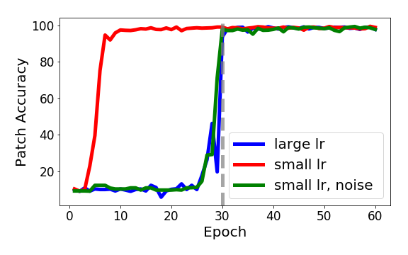
Figure 3: Accuracy vs. epoch on patch-augmented CIFAR-10. The gray line indicates annealing of activation noise and learning rate. Left: Clean validation set. Right: Images containing only the patch.

Our theory suggests that adding noise to the network could be an effective strategy to regularize a small learning rate in practice. We test this empirically by adding small Gaussian noise during training before every activation layer in a WideResNet16 [42] architecture, as our analysis highlights pre-activation noise as a key regularization mechanism of SGD. The noise level is annealed over time. We demonstrate on CIFAR-10 images without data augmentation that this regularization can indeed counteract the negative effects of small learning rate, as we report a 4.72% increase in validation accuracy when adding noise to a small learning rate. Full details are in Section G.1.

We will also empirically demonstrate that the choice of large vs. small initial learning rate can indeed invert the learning order of different example types. We add a memorizable 7 ×\times 7 pixel patch to a subset of CIFAR-10 images following the scenario presented in (1.1), such that around 20% of images have no patch, 16% of images contain only a patch, and 64% contain both CIFAR-10 data and patch. We generate the patches so that they are not easily separable, as in our constructed 𝒬\mathcal{Q}, but they are low in variation and therefore easy to memorize. Precise details on producing the data, including a visualization of the patch, are in Section G.2. We train on the modified dataset using WideResNet16 using 3 methods: large learning rate with annealing at the 30th epoch, small initial learning rate, and small learning rate with noise annealed at the 30th epoch.

Figure 3 depicts the validation accuracy vs. epoch on clean (no patch) and patch-only images. From the plots, it is apparent that the small learning rate picks up the signal in the patch very quickly, whereas the other two methods only memorize the patch after annealing.

From the validation accuracy on clean images, we can deduce that the small learning rate method is indeed learning the CIFAR images using a small fraction of all the available data, as the validation accuracy of a small LR model when training on the full dataset is around 83%, but the validation on clean data after training with the patch is 70%. We provide additional arguments in Section G.2. Our code for these experiments is online at the following link: https://github.com/cwein3/large-lr-code.

8 Conclusion

In this work, we show that the order in which a neural net learns to fit different types of patterns plays a crucial role in generalization. To demonstrate this, we construct a distribution on which models trained with large learning rates generalize provably better than those trained with small learning rates due to learning order. Our analysis reveals that more SGD noise, or larger learning rate, biases the model towards learning “generalizing” kernels rather than “memorizing” kernels. We confirm on articifially modified CIFAR-10 data that the scale of the learning rate can indeed influence learning order and generalization. Inspired by these findings, we propose a mitigation strategy that injects noise before the activations and works both theoretically for our construction and empirically. The design of better algorithms for regularizing learning order is an exciting question for future work.

Acknowledgements

CW acknowledges support from a NSF Graduate Research Fellowship.

References

  • Allen-Zhu and Li [2019a] Zeyuan Allen-Zhu and Yuanzhi Li. Can SGD learn recurrent neural networks with provable generalization? CoRR, abs/1902.01028, 2019a. URL http://arxiv.org/abs/1902.01028.
  • Allen-Zhu and Li [2019b] Zeyuan Allen-Zhu and Yuanzhi Li. What can resnet learn efficiently, going beyond kernels? CoRR, abs/1905.10337, 2019b. URL http://arxiv.org/abs/1905.10337.
  • Allen-Zhu et al. [2018] Zeyuan Allen-Zhu, Yuanzhi Li, and Yingyu Liang. Learning and Generalization in Overparameterized Neural Networks, Going Beyond Two Layers. arXiv preprint arXiv:1811.04918, November 2018.
  • Allen-Zhu et al. [2018] Zeyuan Allen-Zhu, Yuanzhi Li, and Zhao Song. On the convergence rate of training recurrent neural networks. arXiv preprint arXiv:1810.12065, 2018.
  • Allen-Zhu et al. [2018a] Zeyuan Allen-Zhu, Yuanzhi Li, and Zhao Song. On the convergence rate of training recurrent neural networks. arXiv preprint arXiv:1810.12065, 2018a.
  • Allen-Zhu et al. [2018b] Zeyuan Allen-Zhu, Yuanzhi Li, and Zhao Song. A convergence theory for deep learning via over-parameterization. arXiv preprint arXiv:1811.03962, November 2018b.
  • Arora et al. [2019] Sanjeev Arora, Simon S. Du, Wei Hu, Zhiyuan Li, and Ruosong Wang. Fine-grained analysis of optimization and generalization for overparameterized two-layer neural networks. CoRR, abs/1901.08584, 2019. URL http://arxiv.org/abs/1901.08584.
  • Bartlett and Mendelson [2002] Peter L Bartlett and Shahar Mendelson. Rademacher and gaussian complexities: Risk bounds and structural results. Journal of Machine Learning Research, 3(Nov):463–482, 2002.
  • Bousquet and Elisseeff [2002] Olivier Bousquet and André Elisseeff. Stability and generalization. Journal of machine learning research, 2(Mar):499–526, 2002.
  • Chen and Gu [2018] Jinghui Chen and Quanquan Gu. Closing the generalization gap of adaptive gradient methods in training deep neural networks. arXiv preprint arXiv:1806.06763, 2018.
  • Dai and Zhu [2018] Xiaowu Dai and Yuhua Zhu. Towards theoretical understanding of large batch training in stochastic gradient descent. arXiv preprint arXiv:1812.00542, 2018.
  • Du et al. [2018a] Simon S. Du, Jason D. Lee, Yuandong Tian, Barnabás Póczos, and Aarti Singh. Gradient descent learns one-hidden-layer CNN: don’t be afraid of spurious local minima. In International Conference on Machine Learning (ICML). http://arxiv.org/abs/1712.00779, 2018a.
  • Du et al. [2018b] Simon S. Du, Xiyu Zhai, Barnabas Poczos, and Aarti Singh. Gradient Descent Provably Optimizes Over-parameterized Neural Networks. ArXiv e-prints, 2018b.
  • Duchi et al. [2011] John Duchi, Elad Hazan, and Yoram Singer. Adaptive subgradient methods for online learning and stochastic optimization. Journal of Machine Learning Research, 12(Jul):2121–2159, 2011.
  • Ge et al. [2019] Rong Ge, Sham M. Kakade, Rahul Kidambi, and Praneeth Netrapalli. The Step Decay Schedule: A Near Optimal, Geometrically Decaying Learning Rate Procedure. arXiv e-prints, art. arXiv:1904.12838, Apr 2019.
  • Goyal et al. [2017] Priya Goyal, Piotr Dollár, Ross Girshick, Pieter Noordhuis, Lukasz Wesolowski, Aapo Kyrola, Andrew Tulloch, Yangqing Jia, and Kaiming He. Accurate, large minibatch sgd: Training imagenet in 1 hour. arXiv preprint arXiv:1706.02677, 2017.
  • He et al. [2016] Kaiming He, Xiangyu Zhang, Shaoqing Ren, and Jian Sun. Deep residual learning for image recognition. In Proceedings of the IEEE conference on computer vision and pattern recognition, pages 770–778, 2016.
  • Hoffer et al. [2017] Elad Hoffer, Itay Hubara, and Daniel Soudry. Train longer, generalize better: closing the generalization gap in large batch training of neural networks. In Advances in Neural Information Processing Systems, pages 1731–1741, 2017.
  • Hu et al. [2017] Wenqing Hu, Chris Junchi Li, Lei Li, and Jian-Guo Liu. On the diffusion approximation of nonconvex stochastic gradient descent. arXiv preprint arXiv:1705.07562, 2017.
  • Jastrzębski et al. [2018] Stanisław Jastrzębski, Zachary Kenton, Nicolas Ballas, Asja Fischer, Yoshua Bengio, and Amos Storkey. Dnn’s sharpest directions along the sgd trajectory. arXiv preprint arXiv:1807.05031, 2018.
  • Keskar and Socher [2017] Nitish Shirish Keskar and Richard Socher. Improving generalization performance by switching from adam to sgd. arXiv preprint arXiv:1712.07628, 2017.
  • Keskar et al. [2016] Nitish Shirish Keskar, Dheevatsa Mudigere, Jorge Nocedal, Mikhail Smelyanskiy, and Ping Tak Peter Tang. On large-batch training for deep learning: Generalization gap and sharp minima. arXiv preprint arXiv:1609.04836, 2016.
  • Kingma and Ba [2014] Diederik P Kingma and Jimmy Ba. Adam: A method for stochastic optimization. arXiv preprint arXiv:1412.6980, 2014.
  • Kleinberg et al. [2018] Robert Kleinberg, Yuanzhi Li, and Yang Yuan. An alternative view: When does SGD escape local minima? CoRR, abs/1802.06175, 2018. URL http://arxiv.org/abs/1802.06175.
  • Krizhevsky et al. [2012] Alex Krizhevsky, Ilya Sutskever, and Geoffrey E Hinton. Imagenet classification with deep convolutional neural networks. In Advances in neural information processing systems, pages 1097–1105, 2012.
  • Li and Liang [2018] Yuanzhi Li and Yingyu Liang. Learning overparameterized neural networks via stochastic gradient descent on structured data. In Advances in Neural Information Processing Systems, pages 8157–8166, 2018.
  • Li et al. [2017] Yuanzhi Li, Tengyu Ma, and Hongyang Zhang. Algorithmic regularization in over-parameterized matrix recovery. CoRR, abs/1712.09203, 2017. URL http://arxiv.org/abs/1712.09203.
  • Loshchilov and Hutter [2016] Ilya Loshchilov and Frank Hutter. Sgdr: Stochastic gradient descent with warm restarts. arXiv preprint arXiv:1608.03983, 2016.
  • Luo et al. [2019] Liangchen Luo, Yuanhao Xiong, Yan Liu, and Xu Sun. Adaptive gradient methods with dynamic bound of learning rate. arXiv preprint arXiv:1902.09843, 2019.
  • Mangalam and Prabhu [2019] Karttikeya Mangalam and Vinay Prabhu. Do deep neural networks learn shallow learnable examples first? June 2019.
  • Nakkiran et al. [2019] Preetum Nakkiran, Gal Kaplun, Dimitris Kalimeris, Tristan Yang, Benjamin L. Edelman, Fred Zhang, and Boaz Barak. SGD on Neural Networks Learns Functions of Increasing Complexity. arXiv e-prints, art. arXiv:1905.11604, May 2019.
  • Simonyan and Zisserman [2014] Karen Simonyan and Andrew Zisserman. Very deep convolutional networks for large-scale image recognition. arXiv preprint arXiv:1409.1556, 2014.
  • Smith [2017] Leslie N Smith. Cyclical learning rates for training neural networks. In 2017 IEEE Winter Conference on Applications of Computer Vision (WACV), pages 464–472. IEEE, 2017.
  • Smith and Le [2017] Samuel L Smith and Quoc V Le. A bayesian perspective on generalization and stochastic gradient descent. arXiv preprint arXiv:1710.06451, 2017.
  • Smith et al. [2017] Samuel L Smith, Pieter-Jan Kindermans, Chris Ying, and Quoc V Le. Don’t decay the learning rate, increase the batch size. arXiv preprint arXiv:1711.00489, 2017.
  • Soudry et al. [2018] Daniel Soudry, Elad Hoffer, Mor Shpigel Nacson, Suriya Gunasekar, and Nathan Srebro. The implicit bias of gradient descent on separable data. The Journal of Machine Learning Research, 19(1):2822–2878, 2018.
  • Tieleman and Hinton [2012] Tijmen Tieleman and Geoffrey Hinton. Lecture 6.5-rmsprop, coursera: Neural networks for machine learning. University of Toronto, Technical Report, 2012.
  • Wen et al. [2019] Yeming Wen, Kevin Luk, Maxime Gazeau, Guodong Zhang, Harris Chan, and Jimmy Ba. Interplay between optimization and generalization of stochastic gradient descent with covariance noise. arXiv preprint arXiv:1902.08234, 2019.
  • Wilson et al. [2017] Ashia C Wilson, Rebecca Roelofs, Mitchell Stern, Nati Srebro, and Benjamin Recht. The marginal value of adaptive gradient methods in machine learning. In Advances in Neural Information Processing Systems, pages 4148–4158, 2017.
  • Xing et al. [2018] Chen Xing, Devansh Arpit, Christos Tsirigotis, and Yoshua Bengio. A walk with sgd. arXiv preprint arXiv:1802.08770, 2018.
  • You et al. [2017] Yang You, Igor Gitman, and Boris Ginsburg. Large batch training of convolutional networks. arXiv preprint arXiv:1708.03888, 2017.
  • Zagoruyko and Komodakis [2016] Sergey Zagoruyko and Nikos Komodakis. Wide residual networks. arXiv preprint arXiv:1605.07146, 2016.
  • Zeiler [2012] Matthew D Zeiler. Adadelta: an adaptive learning rate method. arXiv preprint arXiv:1212.5701, 2012.

Appendix A Basic Properties and Toolbox

In this section, we collect a few basic properties of the neural networks we are studying. In section F, we provide two lemmas on Gaussian random variables and perturbation theory of the matrices.

Proposition A.1.
[∇L^​(U)]i=𝔼^​[ℓ′​(f⁡(u,U,(x,y)))​𝟙​([U]i​x)​x]\displaystyle[\nabla\widehat{L}(U)]_{i}=\widehat{\mathbb{E}}\left[\ell^{\prime}(f(u,U;(x,y)))\mathbbm{1}([U]_{i}x)x\right] (A.1)
Proposition A.2.

Let [∇L^​(U)]i[\nabla\widehat{L}(U)]_{i} be the ii-th row of ∇L^​(U)\nabla\widehat{L}(U). We have that ‖[∇L^​(U)]i‖2≲1/m\|[\nabla\widehat{L}(U)]_{i}\|_{2}\lesssim 1/\sqrt{m}.

Proposition A.3.

For any tt, if γs=η\gamma_{s}=\eta for every s≤ts\leq t, then we have that ‖[U¯t]i‖2≲min⁡{1m​λ,η​t/m}\|[\overline{U}_{t}]_{i}\|_{2}\lesssim\min\{\frac{1}{\sqrt{m}\lambda},\eta t/\sqrt{m}\} and ‖U¯t‖F≲1λ\|\overline{U}_{t}\|_{F}\lesssim\frac{1}{\lambda}.

Proof.

By equation (3.4) and Proposition A.2, we have that

‖[U¯t]i‖2=∑sη​(1−η​λ)t−s​‖[∇L^​(Us)]i‖2≤1m​∑sη​(1−η​λ)t−s≲min⁡{1m​λ,η​tm}\|[\overline{U}_{t}]_{i}\|_{2}=\sum_{s}\eta(1-\eta\lambda)^{t-s}\|[\nabla\widehat{L}(U_{s})]_{i}\|_{2}\leq\frac{1}{\sqrt{m}}\sum_{s}\eta(1-\eta\lambda)^{t-s}\lesssim\min\left\{\frac{1}{\sqrt{m}\lambda},\frac{\eta t}{\sqrt{m}}\right\}

∎

Proposition A.4.

Suppose that matrix U~∈ℝm×d\widetilde{U}\in\mathbb{R}^{m\times d} is a random variable whose columns have i.i.d distribution 𝒩⁡(0,τ2​Im×m)\mathcal{N}(0,\tau^{2}I_{m\times m}) and u∈ℝmu\in\mathbb{R}^{m} such that each entry of uu is i.i.d. uniform in {−m−1/2,m1/2}\{-m^{-1/2},m^{1/2}\}.For every xx, we have that w.h.p. over the randomness of U~\widetilde{U} and uu that

|NU~​(u,U~,x)|≲τ​‖x‖2​log⁡d\displaystyle\left|N_{\widetilde{U}}(u,\widetilde{U};x)\right|\lesssim\tau\|x\|_{2}\log d (A.2)
Proof of Proposition A.4.

By definition, we have that

NU~​(u,U~,x)\displaystyle N_{\widetilde{U}}(u,\widetilde{U};x) =∑i∈[m]ui​[[U~]i​x]+\displaystyle=\sum_{i\in[m]}u_{i}[[\widetilde{U}]_{i}x]_{+} (A.3)

By definition, U~∈ℝm×d\widetilde{U}\in\mathbb{R}^{m\times d} where each entry is i.i.d. 𝒩⁡(0,τ2)\mathcal{N}(0,\tau^{2}), which implies that when m≥dm\geq d, w.h.p. ‖U~‖2=O⁡(τ​m)\|\widetilde{U}\|_{2}=O(\tau\sqrt{m}).

Hence ‖[U~​x]+‖2≤‖U~​x‖2≲τ​m​‖x‖2\|[\widetilde{U}x]_{+}\|_{2}\leq\|\widetilde{U}x\|_{2}\lesssim\tau\sqrt{m}\|x\|_{2}. Now, since each uiu_{i} is i.i.d. uniform {−m−1/2,m1/2}\{-m^{-1/2},m^{1/2}\}, using the randomness of uiu_{i} we know that w.h.p.

|∑i∈[m]ui​[[U~]i​x]+|≲log⁡mm​‖[U~​x]+‖2≲τ​‖x‖2​log⁡d\displaystyle\left|\sum_{i\in[m]}u_{i}[[\widetilde{U}]_{i}x]_{+}\right|\lesssim\frac{\log m}{\sqrt{m}}\|[\widetilde{U}x]_{+}\|_{2}\lesssim\tau\|x\|_{2}\log d (A.4)

∎

Proposition A.5.

Under the same setting as Lemma A.8, we will also have w.h.p over the randomness of U~\widetilde{U} and uu, ∀U¯∈ℝd×m\forall\overline{U}\in\mathbb{R}^{d\times m},

|NU(u,U~;x)−NU~(u,U~;x)|≲B∥U¯∥F5/3τ−2/3m−1/6\displaystyle\left|N_{U}(u,\widetilde{U};x)-N_{\widetilde{U}}(u,\widetilde{U};x)\right|\lesssim B\|\overline{U}\|_{F}^{5/3}\tau^{-2/3}m^{-1/6} (A.5)

Thus, it also follows that

|NU(u,U~;x)|≲B∥U¯∥F5/3τ−2/3m−1/6+τBlogd\displaystyle|N_{U}(u,\widetilde{U};x)|\lesssim B\|\overline{U}\|_{F}^{5/3}\tau^{-2/3}m^{-1/6}+\tau B\log d (A.6)
Proof.

We know that for every ii where 𝟙​([U]i​x)≠𝟙​([U~]i​x)\mathbbm{1}([U]_{i}x)\not=\mathbbm{1}([\widetilde{U}]_{i}x), it holds that |[U~]i​x|≤|[U¯]i​x||[\widetilde{U}]_{i}x|\leq|[\overline{U}]_{i}x|. This implies that

|NU​(u,U~,x)−NU~​(u,U~,x)|\displaystyle\left|N_{U}(u,\widetilde{U};x)-N_{\widetilde{U}}(u,\widetilde{U};x)\right| ≤1m​∑i∈[m]|𝟙​([U]i​x)−𝟙​([U~]i​x)|​|[U¯]i​x|\displaystyle\leq\frac{1}{\sqrt{m}}\sum_{i\in[m]}|\mathbbm{1}([U]_{i}x)-\mathbbm{1}([\widetilde{U}]_{i}x)||[\overline{U}]_{i}x| (A.7)
≤1m​‖𝟙​(U​x)−𝟙​(U~​x)‖1​maxi​|[U¯]i​x|\displaystyle\leq\frac{1}{\sqrt{m}}\|\mathbbm{1}(Ux)-\mathbbm{1}(\widetilde{U}x)\|_{1}\max_{i}|[\overline{U}]_{i}x| (A.8)
≲B∥U¯∥F4/3τ−4/3m1/6maxi∥[U¯]i∥2\displaystyle\lesssim B\|\overline{U}\|_{F}^{4/3}\tau^{-4/3}m^{1/6}\max_{i}\|[\overline{U}]_{i}\|_{2} (A.9)

Here in the last inequality we applied Lemma A.8. The second statement follows from Proposition A.4 and triangle inequality. ∎

We have the following Rademacher complexity bound:

Lemma A.6 (Lemma G5 and 5.9 of [3]).

Let U=U¯+U~U=\overline{U}+\widetilde{U}, where U~∈ℝm×d\widetilde{U}\in\mathbb{R}^{m\times d} is a random variable whose columns have i.i.d distribution 𝒩⁡(0,τ02​Im×m)\mathcal{N}(0,\tau_{0}^{2}I_{m\times m}) and u∈ℝmu\in\mathbb{R}^{m} such that each entry of uu is i.i.d. uniform in {−m−1/2,m1/2}\{-m^{-1/2},m^{1/2}\}. W.h.p. over the samples {x(i)}\{x^{(i)}\} and the randomness of u,U~u,\widetilde{U}, we have that for every ρ∈[0,1/λ]\rho\in[0,1/\lambda]:

ℛ\displaystyle\mathcal{R} :=1N​∑i∈[N]𝔼σ​[|sup‖U¯‖F2≤ρ2σi​NU​(u,U¯,x(i))|]≤O⁡(ρ+εs)\displaystyle:=\frac{1}{\sqrt{N}}\sum_{i\in[N]}\mathbb{E}_{\sigma}\left[\left|\sup_{\|\bar{U}\|_{F}^{2}\leq\rho^{2}}\sigma_{i}N_{U}(u,\bar{U};x^{(i)})\right|\right]\leq{O}(\rho+\varepsilon_{s}) (A.10)

A.1 Preliminaries on Decoupling the Iterates

In this section, we collect useful statements which will help with decoupling the signal U¯\overline{U} from the noise U~\widetilde{U} in our analysis. First, we observe that if the noise updates in the system stabilize at initialization, the marginal distribution of UtU_{t} is always the same as the initialization.

Proposition A.7.

Under Assumption 3.1, suppose we run Algorithm 1. Then for any tt before annealing the learning rate, U~t\widetilde{U}_{t} has marginal distribution 𝒩⁡(0,τ02​Im×m⊗Id×d)\mathcal{N}(0,\tau_{0}^{2}I_{m\times m}\otimes I_{d\times d}). In other words, each entry of U~t\widetilde{U}_{t} follows 𝒩⁡(0,τ02)\mathcal{N}(0,\tau_{0}^{2}) and they are independent with each others.

One nice aspect of the signal-noise decomposition is as follows: we use tools from [6] to show that if the signal term U¯\overline{U} is small, then using only the noise component U~\widetilde{U} to compute the activations roughly preserves the output of the network. This facilitates our analysis of the network dynamics.

Lemma A.8.

[Lemma 5.2 of [6]] Let x∈ℝdx\in\mathbb{R}^{d} be a fixed example with ‖x‖2≤B\|x\|_{2}\leq B. For every τ>0\tau>0, let U=U¯+U~U=\overline{U}+\widetilde{U} where U~∈ℝm×d\widetilde{U}\in\mathbb{R}^{m\times d} is a random variable whose columns have i.i.d distribution 𝒩⁡(0,τ2​Im×m)\mathcal{N}(0,\tau^{2}I_{m\times m}) and u∈ℝmu\in\mathbb{R}^{m} such that each entry of uu is i.i.d. uniform in {−m−1/2,m1/2}\{-m^{-1/2},m^{1/2}\}. We have that, w.h.p over the randomness of U~\widetilde{U} and uu, ∀U¯∈ℝd×m\forall\overline{U}\in\mathbb{R}^{d\times m},

|NU(u,U¯;x)−NU~(u,U¯;x)|≲B∥U¯∥Fτ−2m−1/6\displaystyle\left|N_{U}(u,\overline{U};x)-N_{\widetilde{U}}(u,\overline{U};x)\right|\lesssim B\|\overline{U}\|_{F}\tau^{-2}m^{-1/6} (A.11)

Moreover, we have that ∥𝟙(Ux)−𝟙(U~x)∥1≲∥U¯∥F4/3τ−4/3m2/3\|\mathbbm{1}(Ux)-\mathbbm{1}(\widetilde{U}x)\|_{1}\lesssim\|\overline{U}\|_{F}^{4/3}\tau^{-4/3}m^{2/3}.

As we will often apply (A.11) with ‖U¯‖F≲1λ\|\overline{U}\|_{F}\lesssim\frac{1}{\lambda}, for notational simplicity we denote throughout the paper εs=(1λ​τ0)4/3m−1/3\varepsilon_{s}=\left(\frac{1}{\lambda\tau_{0}}\right)^{4/3}m^{-1/3}. By our choice of m≥poly​(d/τ0)m\geq\textup{poly}(d/\tau_{0}) we know that εs≤d−Θ⁡(1)\varepsilon_{s}\leq d^{-\Theta(1)}.

Appendix B Proof of Main Theorems

B.1 Proof of Theorem 3.4

We start with the following lemma that shows that if gg has small training error on ℳ¯1\bar{\mathcal{M}}_{1}, then the output of gg on x2x_{2} is large compared to ‖x2‖\|x_{2}\|. This is because for the loss to be low, gg must have a good margin on x2x_{2}. However, as the norm of x2x_{2} is roughly uniform in [0,1][0,1], the examples with small norm will force gg to have larger output.

Lemma B.1 (Signal of gg).

W.h.p. for every t≥0t\geq 0 and every δ≥1q​N\delta\geq\frac{1}{\sqrt{qN}}, as long as L^ℳ¯1​(gt0+t)≤δ\widehat{L}_{\bar{\mathcal{M}}_{1}}(g_{t_{0}+t})\leq\delta, we have that: for every (x,y)(x,y),

y​gt0+t​(x2)≳‖x‖2δ\displaystyle yg_{t_{0}+t}(x_{2})\gtrsim\frac{\|x\|_{2}}{\delta} (B.1)
Proof of Lemma B.1.

We use ℳ¯1(1)\bar{\mathcal{M}}_{1}^{(1)} to denote the set of all x2(i)∈ℳ¯1x_{2}^{(i)}\in\bar{\mathcal{M}}_{1} such that x2(i)=α⁡(z−ζ)x_{2}^{(i)}=\alpha(z-\zeta). Similarly, we use ℳ¯1(2)\bar{\mathcal{M}}_{1}^{(2)} to denote the set of all x2(i)∈ℳ¯1x_{2}^{(i)}\in\bar{\mathcal{M}}_{1} such that x2(i)=α⁡(z+ζ)x_{2}^{(i)}=\alpha(z+\zeta), and use ℳ¯1(3)\bar{\mathcal{M}}_{1}^{(3)} to denote the set of all x2(i)∈ℳ¯1x_{2}^{(i)}\in\bar{\mathcal{M}}_{1} such that x2(i)=α​zx_{2}^{(i)}=\alpha z.

Let gt0+t​(z+ζ)=ρ1,gt0+t​(z−ζ)=ρ2,gt+t0​(z)=ρ3g_{t_{0}+t}(z+\zeta)=\rho_{1},g_{t_{0}+t}(z-\zeta)=\rho_{2},g_{t+t_{0}}(z)=\rho_{3}. By the positive homogeneity of ReLU, we know that for every x2∈ℳ¯1(i)x_{2}\in\bar{\mathcal{M}}_{1}^{(i)}, it holds:

gt0+t​(x2)=‖x2‖2​ρi\displaystyle g_{t_{0}+t}(x_{2})=\|x_{2}\|_{2}\rho_{i} (B.2)

Since L^ℳ¯1​(gt0+t)≤δ\widehat{L}_{\bar{\mathcal{M}}_{1}}(g_{t_{0}+t})\leq\delta, it holds that w.h.p. for every i∈[3]i\in[3],

L^ℳ¯1(i)​(gt0+t)≤4​δ\displaystyle\widehat{L}_{\bar{\mathcal{M}}_{1}^{(i)}}(g_{t_{0}+t})\leq 4\delta (B.3)

Hence, at most 40​δ40\delta fraction of x2∈ℳ¯1(i)x_{2}\in\bar{\mathcal{M}}_{1}^{(i)} satisfies ℓ⁡(gt0+t,(x2,y))≥110\ell(g_{t_{0}+t};(x_{2},y))\geq\frac{1}{10}. Since ‖x2‖2\|x_{2}\|_{2} is uniform on [0,1][0,1], this implies that as long as δ≥1q​N\delta\geq\frac{1}{\sqrt{qN}}, w.h.p., 80​δ80\delta fraction of the x2∈ℳ¯1(i)x_{2}\in\bar{\mathcal{M}}_{1}^{(i)} satisfies that ‖x2‖2=O⁡(δ)\|x_{2}\|_{2}=O(\delta). Among of these examples, at least 40​δ40\delta fraction of them should satisfy ℓ⁡(gt0+t,(x2,y))≤110\ell(g_{t_{0}+t};(x_{2},y))\leq\frac{1}{10}, which implies that ‖x2‖​ρi≳1\|x_{2}\|\rho_{i}\gtrsim 1. This implies that ρi≳1/δ\rho_{i}\gtrsim 1/\delta and the conclusion follows from equality (B.2).

∎

Our proof of Theorem 3.4 now amounts to carefully checking that all examples in ℳ2\mathcal{M}_{2} are classified correctly, and the classifier rt0+tr_{t_{0}+t} will generalize well on ℳ¯2\bar{\mathcal{M}}_{2}.

Proof of Theorem 3.4.

By Lemma 4.4, we know that for t=O~​(1ε13​η2​r)t=\widetilde{O}\left(\frac{1}{\varepsilon_{1}^{3}\eta_{2}r}\right) we have L^ℳ¯1​(gt0+t)=O⁡(ε1/q3)\widehat{L}_{\bar{\mathcal{M}}_{1}}(g_{t_{0}+t})=O(\sqrt{\varepsilon_{1}/q^{3}}). Thus applying Lemma B.1, we obtain that as long as ε1≥1N\varepsilon_{1}\geq\frac{1}{\sqrt{N}} (which is implied by Assumption 3.3)

y​gt0+t​(x2)≥Ω⁡(‖x‖2​q3ε1)\displaystyle yg_{t_{0}+t}(x_{2})\geq{\Omega}\left(\frac{\|x\|_{2}\sqrt{q^{3}}}{\sqrt{\varepsilon_{1}}}\right) (B.4)

On the other hand for rt0+tr_{t_{0}+t}, by Lemma 4.1 and Lemma 4.3 we know that ‖W¯t0+t‖F=O~​(d)\|\overline{W}_{t_{0}+t}\|_{F}=\widetilde{O}(\sqrt{d}). Let us define 𝒟x1\mathcal{D}_{x_{1}} to be the marginal distribution of x1x_{1}. We know that x1=α​w⋆+βx_{1}=\alpha w^{\star}+\beta where w.h.p. |α|=O~(d−1/2)|\alpha|=\tilde{O}(d^{-1/2}) and β∼𝒩⁡(0,1/d×(I−w⋆​(w⋆)⊤))\beta\sim\mathcal{N}(0,1/d\times(I-w^{\star}(w^{\star})^{\top})). Hence we have that w.h.p. over x1∼𝒟x1x_{1}\sim\mathcal{D}_{x_{1}}, ∥W¯t0+tx1∥2≤|α|∥W¯t0+t∥F+d−1/2∥β∥2∥W¯t0+t∥F≤O~(d−1/2)∥W¯t0+t∥F≤O~(1)\|\overline{W}_{t_{0}+t}x_{1}\|_{2}\leq|\alpha|\|\overline{W}_{t_{0}+t}\|_{F}+d^{-1/2}\|\beta\|_{2}\|\overline{W}_{t_{0}+t}\|_{F}\leq\widetilde{O}(d^{-1/2})\|\overline{W}_{t_{0}+t}\|_{F}\leq\widetilde{O}(1).

This implies that for x1∼𝒟x1x_{1}\sim\mathcal{D}_{x_{1}}, applying Lemma A.8 gives us

|rt0+t​(x1)|\displaystyle|r_{t_{0}+t}(x_{1})| =|NUt0+t​(u,Ut0+t,x1)|\displaystyle=|N_{U_{t_{0}+t}}(u,U_{t_{0}+t};x_{1})| (B.5)
≲|NUt0+t​(u,U¯t0+t,x1)|+εsλ+τ0​log⁡d\displaystyle\lesssim|N_{U_{t_{0}+t}}(u,\overline{U}_{t_{0}+t};x_{1})|+\frac{\varepsilon_{s}}{\lambda}+\tau_{0}\log d (by Proposition A.5)
≲‖u‖2​‖W¯t0+t​x1‖2+εsλ+τ0​log⁡d=O~​(1)\displaystyle\lesssim\|u\|_{2}\|\overline{W}_{t_{0}+t}x_{1}\|_{2}+\frac{\varepsilon_{s}}{\lambda}+\tau_{0}\log d=\widetilde{O}(1) (by our choice of τ0\tau_{0}, mm)

Hence as long as ‖x2‖2=Ω~​(ε1/q3​log⁡1ε1)\|x_{2}\|_{2}=\tilde{\Omega}(\sqrt{\varepsilon_{1}/q^{3}}\log\frac{1}{\varepsilon_{1}}), it holds that

y⁡(rt0+t​(x1)+gt0+t​(x2))=Ω~​(1)×log⁡1ε1\displaystyle y(r_{t_{0}+t}(x_{1})+g_{t_{0}+t}(x_{2}))=\tilde{\Omega}(1)\times\log\frac{1}{\varepsilon_{1}} (B.6)

This implies that ℓ⁡(rt0+t+gt0+t,(x,y))≤ε1\ell(r_{t_{0}+t}+g_{t_{0}+t};(x,y))\leq\varepsilon_{1}. Otherwise, when ‖x2‖2=O~​(ε1/q3)\|x_{2}\|_{2}=\widetilde{O}\left(\sqrt{\varepsilon_{1}/q^{3}}\right), we also know that w.h.p. ℓ⁡(rt0+t+gt0+t,(x,y))≤ℓ⁡(rt0+t,(x,y))=O~​(1)\ell(r_{t_{0}+t}+g_{t_{0}+t};(x,y))\leq\ell(r_{t_{0}+t};(x,y))=\tilde{O}(1), since y​gt0+t​(x2)≥0yg_{t_{0}+t}(x_{2})\geq 0. On the other hand by Lemma 4.4, we also know that

L^ℳ1​(rt0+t)\displaystyle\widehat{L}_{\mathcal{M}_{1}}(r_{t_{0}+t}) =O⁡(ε1/q)\displaystyle=O(\sqrt{\varepsilon_{1}/q}) (B.7)

Moreover, applying Lemma A.6 on rt0+tr_{t_{0}+t} with ‖Wt0+t‖F2≤‖Wt0‖F2+‖Wt0+t−Wt0‖F2≲(d​log2​1ε)\|W_{t_{0}+t}\|_{F}^{2}\leq\|W_{t_{0}}\|_{F}^{2}+\|W_{t_{0}+t}-W_{t_{0}}\|_{F}^{2}\lesssim\left(d\log^{2}\frac{1}{\varepsilon}\right) by Lemma 4.2 and Lemma 4.3, we have that

𝔼(x,y)∼𝒟​[ℓ⁡(rt0+t,(x,y))∣x1≠0]≲ε1/q+κ​log​1ε1≲κ​log​1ε1\displaystyle\mathbb{E}_{(x,y)\sim\mathcal{D}}\left[\ell(r_{t_{0}+t};(x,y))\mid x_{1}\not=0\right]\lesssim\sqrt{\varepsilon_{1}/q}+\kappa\log\frac{1}{\varepsilon_{1}}\lesssim\kappa\log\frac{1}{\varepsilon_{1}} (B.8)

where we used the fact that ε1≤κ2​p2​q3\varepsilon_{1}\leq\kappa^{2}p^{2}q^{3}.

It follows thats

𝔼⁡[ℓ⁡(rt0+t+gt0+t,(x,y))]\displaystyle\mathbb{E}\left[\ell(r_{t_{0}+t}+g_{t_{0}+t};(x,y))\right] (B.9)
≤Pr[x2=0]𝔼[ℓ(rt0+t;(x,y))]+Pr[x2≠0]𝔼[ℓ(rt0+t+gt0+t;(x,y))]\displaystyle\leq\Pr[x_{2}=0]\mathbb{E}\left[\ell(r_{t_{0}+t};(x,y))\right]+\Pr[x_{2}\not=0]\mathbb{E}\left[\ell(r_{t_{0}+t}+g_{t_{0}+t};(x,y))\right] (B.10)
≤𝔼[ℓ(rt0+t;(x,y))∣x1≠0]Pr[x2=0]+O~(1)Pr[x2≠0,∥x2∥2=O(ε1/q3)]+ε1\displaystyle\leq\mathbb{E}\left[\ell(r_{t_{0}+t};(x,y))\mid x_{1}\not=0\right]\Pr[x_{2}=0]+\widetilde{O}(1)\Pr\left[x_{2}\not=0,\|x_{2}\|_{2}=O\left(\sqrt{\varepsilon_{1}/q^{3}}\right)\right]+\varepsilon_{1} (B.11)
≤O~​(ε1/q3)+ε1≤O⁡(p​κ​log⁡1ε1)\displaystyle\leq\widetilde{O}\left(\sqrt{\varepsilon_{1}/q^{3}}\right)+\varepsilon_{1}\leq O\left(p\kappa\log\frac{1}{\varepsilon_{1}}\right) (B.12)

Here the last step uses the definition of ε1\varepsilon_{1} that ε1≤κ2​p2​q3\varepsilon_{1}\leq\kappa^{2}p^{2}q^{3}. ∎

B.2 Proof of Theorem 3.5

We will prove Theorem 3.5 using Lemma 5.3 by roughly arguing that the predictions made by rtr_{t} will be heavily influenced by a vector α\alpha in the low rank span of examples from ℳ¯2\bar{\mathcal{M}}_{2}. With high probability, this vector α\alpha will be noisy and not align well with the ground truth w⋆w^{\star}, leading to mispredictions.

Proof of Theorem 3.5.

Recall that ε2′\varepsilon_{2}^{\prime} denotes the stopping criterion used in Theorem 3.5 and ε3=d−1/321ε2′2\varepsilon_{3}=d^{-1/32}\frac{1}{\varepsilon_{2}^{\prime 2}}. Using Lemma 5.3, we know that w.h.p.

rt​(x1)−rt​(−x1)=2​⟨α,x1⟩±O~​(ε3)\displaystyle r_{t}(x_{1})-r_{t}(-x_{1})=2\langle\alpha,x_{1}\rangle\pm\widetilde{O}\left(\varepsilon_{3}\right) (B.13)

Consider the matrix M=(x1(i))i∈ℳ¯2∈ℝd×N​pM=(x_{1}^{(i)})_{i\in\bar{\mathcal{M}}_{2}}\in\mathbb{R}^{d\times Np}. By definition, we know that M=M0+M1M=M_{0}+M_{1} where M0=w⋆​β⊤M_{0}=w^{\star}\beta^{\top} where βi∈{−d−1/2,d−1/2}\beta_{i}\in\{-d^{-1/2},d^{-1/2}\} and M1M_{1} is a Gaussian random matrix with each entry i.i.d. 𝒩⁡(0,1/d)\mathcal{N}(0,1/d).

By Lemma F.2 we know that w.h.p. over the randomness of x1(i)x_{1}^{(i)}’s, for α∈span​{x1(i)}i∈ℳ¯2\alpha\in\text{span}\{x_{1}^{(i)}\}_{i\in\bar{\mathcal{M}}_{2}} we have as long as N​p≤d/2Np\leq d/2: ⟨α,w⋆⟩‖α‖2​‖w⋆‖2≤0.9\frac{\langle\alpha,w^{\star}\rangle}{\|\alpha\|_{2}\|w^{\star}\|_{2}}\leq 0.9. For every randomly chosen x1x_{1}, we can also write x1=γ​w⋆+βx_{1}=\gamma w^{\star}+\beta where β⊥w⋆\beta\bot w^{\star} so β\beta is independent of γ\gamma, hence

⟨α,x1⟩=γ⁡⟨α,w⋆⟩+⟨α,β⟩\displaystyle\langle\alpha,x_{1}\rangle=\gamma\langle\alpha,w^{\star}\rangle+\langle\alpha,\beta\rangle (B.14)

Note that ⟨α,β⟩∼𝒩⁡(0,σ2​‖α‖22/d)\langle\alpha,\beta\rangle\sim\mathcal{N}(0,\sigma^{2}\|\alpha\|_{2}^{2}/d) with σ≥0.1\sigma\geq 0.1, and with probability at least 0.10.1, γ≤2​‖α‖2/d\gamma\leq 2\|\alpha\|_{2}/\sqrt{d}. This implies that with probability at least Ω⁡(1)\Omega(1) over a randomly chosen x1x_{1} we can have:

⟨w⋆,x1⟩=γ<0,|γ|≤2​‖α‖2/d\displaystyle\langle w^{\star},x_{1}\rangle=\gamma<0,\quad|\gamma|\leq 2\|\alpha\|_{2}/\sqrt{d} (B.15)

For β\beta, we know that with probability at least Ω⁡(1)\Omega(1), we have:

⟨α,β⟩≥3​‖α‖2/d\displaystyle\langle\alpha,\beta\rangle\geq 3\|\alpha\|_{2}/\sqrt{d} (B.16)

Moreover, since β\beta is independent of γ\gamma, we know that with probability Ω⁡(1)\Omega(1) both events can happen, in which case:

⟨w⋆,x1⟩<0,⟨α,x1⟩=γ⁡⟨α,w⋆⟩+⟨α,β⟩≥‖α‖2/d\displaystyle\langle w^{\star},x_{1}\rangle<0,\quad\langle\alpha,x_{1}\rangle=\gamma\langle\alpha,w^{\star}\rangle+\langle\alpha,\beta\rangle\geq\|\alpha\|_{2}/\sqrt{d} (B.17)

Thus, since ‖α‖2=Ω⁡(N​p)\|\alpha\|_{2}=\Omega(\sqrt{Np}) by Lemma 5.3, we know that as long as

pκ=N​pd=Ω~​(ε3)\displaystyle\frac{\sqrt{p}}{\kappa}=\frac{\sqrt{Np}}{\sqrt{d}}=\tilde{\Omega}\left(\varepsilon_{3}\right) (B.18)

which is implied by ε3=O~​(pκ)\varepsilon_{3}=\widetilde{O}\left(\frac{\sqrt{p}}{\kappa}\right), it holds that ⟨α,x1⟩≥Ω~​(ε3)\langle\alpha,x_{1}\rangle\geq\tilde{\Omega}\left(\varepsilon_{3}\right). This implies that

rt​(x1)\displaystyle r_{t}(x_{1}) =rt​(−x1)+2​⟨α,x1⟩±O~​(ε3)\displaystyle=r_{t}(-x_{1})+2\langle\alpha,x_{1}\rangle\pm\widetilde{O}\left(\varepsilon_{3}\right) (B.19)
≥rt​(−x1)\displaystyle\geq r_{t}(-x_{1}) (B.20)

However, since ⟨w⋆,x1⟩<0\langle w^{\star},x_{1}\rangle<0, we know that either rt​(x1)<0r_{t}(x_{1})<0, which results in rt​(−x1)<0r_{t}(-x_{1})<0 but ⟨w⋆,−x1⟩>0\langle w^{\star},-x_{1}\rangle>0. So when x2=0x_{2}=0, the network classifies (−x1,0)(-x_{1},0) incorrectly. On the other hand, we have when rt​(x1)>0r_{t}(x_{1})>0 the network will classify (x1,0)(x_{1},0) incorrectly. Since ⟨w⋆,x1⟩<0\langle w^{\star},x_{1}\rangle<0 and rt​(x1)≥rt​(−x1)r_{t}(x_{1})\geq r_{t}(-x_{1}) holds with probability Ω⁡(1)\Omega(1), this shows that the test error is at least Ω⁡(p)\Omega(p). ∎

Appendix C Proofs for Large Learning Rate Lemmas

C.1 Proofs for Lemma 4.1

To prove Lemma 4.1, we will show that the network will learn all examples with 𝒫\mathcal{P} component while the learning rate is large. The key to the proof is that although the large learning rate noise only allows the network to search over coarse kernels, 𝒫\mathcal{P} is still learnable by these kernels because of its linearly-separable structure. To make this precise, we decompose the weights UtU_{t} Into the signal and noise components, and show that there exists a fixed “target” signal matrix which will classify 𝒫\mathcal{P} correctly no matter the noise matrix.

Recall our definitions of ft​(B,x)f_{t}(B;x), Kt​(B)K_{t}(B) in (6.1) and (6.2), and that

Lt=L^​(Ut)=Kt​(U¯t)\displaystyle L_{t}=\widehat{L}(U_{t})=K_{t}(\overline{U}_{t}) (C.1)
∇UL^​(Ut)=∇Kt​(U¯t)\displaystyle\nabla_{U}\widehat{L}(U_{t})=\nabla K_{t}(\overline{U}_{t}) (C.2)

Recall that Lemma 6.1 leverages the linearly-separable structure of 𝒫\mathcal{P} to find a “target” signal matrix that correctly classifies 𝒫\mathcal{P} w.h.p over the noise matrix. We state its proof below.

Proof of Lemma 6.1.

By proposition A.3, ‖U¯t‖F≤O⁡(1λ)\|\overline{U}_{t}\|_{F}\leq O\left(\frac{1}{\lambda}\right). We apply Lemma A.8 as follows: by Proposition A.7, U~t\widetilde{U}_{t}’s entry has marginal distribution 𝒩⁡(0,τ02)\mathcal{N}(0,\tau_{0}^{2}) and therefore the column of U~t\widetilde{U}_{t} has distribution 𝒩⁡(0,τ02​Im×m)\mathcal{N}(0,\tau_{0}^{2}I_{m\times m}). Since w.h.p. ‖x‖2≲log⁡d\|x\|_{2}\lesssim\sqrt{\log d}, the coupling Lemma A.8 gives

‖𝟙​(Ut​x)−𝟙​(U~t​x)‖0≤εs​m\displaystyle\|\mathbbm{1}(U_{t}x)-\mathbbm{1}(\widetilde{U}_{t}x)\|_{0}\leq\varepsilon_{s}m (C.3)

On the other hand, we also have by Proposition A.5, using the fact that maxi⁡‖[U¯i]‖2≲1m​λ\max_{i}\|[\overline{U}_{i}]\|_{2}\lesssim\frac{1}{\sqrt{m}\lambda}, w.h.p.

|NUt​(u,U~t,x)|≲τ0​log⁡d+εsλ≲τ0​log⁡d\displaystyle\left|N_{U_{t}}(u,\widetilde{U}_{t};x)\right|\lesssim\tau_{0}\log d+\frac{\varepsilon_{s}}{\lambda}\lesssim\tau_{0}\log d (C.4)

Here in the last inequality we used the fact that the network is sufficiently over-parameterized so that εs=O~​(τ0​λ)\varepsilon_{s}=\widetilde{O}(\tau_{0}\lambda).

Using (C.4), noting that our choice of m,λ,τ0m,\lambda,\tau_{0} satisfies τ0​log⁡d=o⁡(ε1)\tau_{0}\log d=o(\varepsilon_{1}), we conclude

|NUt​(u,U~t,x)|≤ε1/20\displaystyle\left|N_{U_{t}}(u,\widetilde{U}_{t};x)\right|\leq\varepsilon_{1}/20 (C.5)

Now, let us consider U∗=(W∗,V∗)U^{*}=(W^{*},V^{*}) given by V∗=0V^{*}=0 and an W∗∈ℝm×dW^{*}\in\mathbb{R}^{m\times d} defined as: for all i∈[m]i\in[m], Wi∗=20​wi​d​w⋆​log⁡1ε1∈ℝdW^{*}_{i}=20w_{i}\sqrt{d}w^{\star}\log\frac{1}{\varepsilon_{1}}\in\mathbb{R}^{d}. We will have ‖U∗‖F2=O⁡(d2​log⁡1ε1)\|U^{*}\|_{F}^{2}=O\left(d^{2}\log\frac{1}{\varepsilon_{1}}\right). We first decompose ft​(U∗,x)f_{t}(U^{*};x) into

ft​(U∗,x)\displaystyle f_{t}(U^{*},x) =NUt​(u,U∗+U~t,x)\displaystyle=N_{U_{t}}(u,U^{*}+\widetilde{U}_{t};x) (C.6)
=NUt​(u,U~t,x)+NUt​(u,U∗,x)\displaystyle=N_{U_{t}}(u,\widetilde{U}_{t};x)+N_{U_{t}}(u,U^{*};x) (C.7)

For the term NUt​(u,U∗,x)N_{U_{t}}(u,U^{*};x), we know that

NUt​(u,U∗,x)\displaystyle N_{U_{t}}(u,U^{*};x) =NWt​(w,W∗,x)=20​⟨w⋆,x1⟩​d​log⁡1ε1×∑i=1m/2wi2​𝟙​([Wt]i​x1)\displaystyle=N_{W_{t}}(w,W^{*};x)=20\langle w^{\star},x_{1}\rangle\sqrt{d}\log\frac{1}{\varepsilon_{1}}\times\sum_{i=1}^{m/2}w_{i}^{2}\mathbbm{1}([W_{t}]_{i}x_{1}) (C.8)
=20​⟨w⋆,x1⟩​d​log⁡1ε1×1m​‖𝟙​(Wt​x1)‖1\displaystyle=20\langle w^{\star},x_{1}\rangle\sqrt{d}\log\frac{1}{\varepsilon_{1}}\times\frac{1}{m}\|\mathbbm{1}(W_{t}x_{1})\|_{1} (C.9)

By Lemma A.8, we know that |𝟙​(Wt​x)−𝟙​(W~t​x)|1≤O⁡(εs​m)\left|\mathbbm{1}(W_{t}x)-\mathbbm{1}(\widetilde{W}_{t}x)\right|_{1}\leq O\left(\varepsilon_{s}m\right) and that 20​⟨w⋆,x1⟩​d​log⁡1ε1≲d​log⁡d20\langle w^{\star},x_{1}\rangle\sqrt{d}\log\frac{1}{\varepsilon_{1}}\lesssim\sqrt{d}\log d, which implies that

NUt​(u,U∗,x)\displaystyle N_{U_{t}}(u,U^{*};x) =20​⟨w⋆,x1⟩​d​log⁡1ε1×1m​‖𝟙​(W~t​x1)‖1±O⁡(d​εs​log⁡d)\displaystyle=20\langle w^{\star},x_{1}\rangle\sqrt{d}\log\frac{1}{\varepsilon_{1}}\times\frac{1}{m}\|\mathbbm{1}(\widetilde{W}_{t}x_{1})\|_{1}\pm O\left(\sqrt{d}\varepsilon_{s}\log d\right) (C.10)

Note that entries of W~t​x1\widetilde{W}_{t}x_{1} are i.i.d. random Bernoulli(1/21/2), thus we know that w.h.p.

2m∥𝟙(W~tx1)∥1=12±O(m−1/2log⁡d)=12±O(m−1/3)\displaystyle\frac{2}{m}\|\mathbbm{1}(\widetilde{W}_{t}x_{1})\|_{1}=\frac{1}{2}\pm O(m^{-1/2}\sqrt{\log d})=\frac{1}{2}\pm O(m^{-1/3}) (C.11)

Thus, by our choice that m−1/3=O(ε1)m^{-1/3}=O(\varepsilon_{1}) and d​εs=O⁡(ε1)\sqrt{d}\varepsilon_{s}=O(\varepsilon_{1}),

|NUt​(u,U∗,x)−5​⟨w⋆,x1⟩​log⁡1ε1|≤ε120\displaystyle\left|N_{U_{t}}(u,U^{*};x)-5\langle w^{\star},x_{1}\rangle\log\frac{1}{\varepsilon_{1}}\right|\leq\frac{\varepsilon_{1}}{20} (C.12)

By (C.5), this also implies that

|NUt​(u,U~t+U∗,x)−5​⟨w⋆,x1⟩​log⁡1ε1|≤ε110\displaystyle\left|N_{U_{t}}(u,\widetilde{U}_{t}+U^{*};x)-5\langle w^{\star},x_{1}\rangle\log\frac{1}{\varepsilon_{1}}\right|\leq\frac{\varepsilon_{1}}{10} (C.13)

By definition of w⋆w^{\star}, we know that

1N​∑i=1Nℓ⁡(5​⟨w⋆,x1(i)⟩​log⁡1ε1,(x(i),y(i)))≤q​log⁡2+ε1/5\displaystyle\frac{1}{N}\sum_{i=1}^{N}\ell\left(5\langle w^{\star},x^{(i)}_{1}\rangle\log\frac{1}{\varepsilon_{1}};(x^{(i)},y^{(i)})\right)\leq q\log 2+\varepsilon_{1}/5 (C.14)

Thus, from the fact that ℓ\ell is 1-Lipschitz, it follows that

Kt​(U∗)≤q​log⁡2+ε1/2\displaystyle K_{t}(U^{*})\leq q\log 2+\varepsilon_{1}/2 (C.15)

∎

Now we wish to argue that even though the noise matrix is changing, gradient descent will still find the fixed target signal matrix U⋆U^{\star}. This leverages the fact that once we fix the activation patterns, we can view each step of the optimization as gradient descent with respect to a convex, but changing, function. Below we provide a proof of Theorem 6.2, which allows for optimization of this changing function.

Proof of Theorem 6.2.

For the sake of contradiction, we assume that Kt​(zt)≥c⋆+μK_{t}(z_{t})\geq c^{\star}+\mu for all t≤Tt\leq T. Using the definition of KtλK_{t}^{\lambda}, we have that the update rule of ztz_{t} can be written as

zt+1\displaystyle z_{t+1} =zt−η∇Kt(zt)−ηλzt\displaystyle=z_{t}-\eta\nabla K_{t}(z_{t})-\eta\lambda z_{t} (C.16)
=(1−ηλ)zt−η∇Kt(zt)\displaystyle=(1-\eta\lambda)z_{t}-\eta\nabla K_{t}(z_{t}) (C.17)

It follows that

‖zt+1−z⋆‖22\displaystyle\|z_{t+1}-z^{\star}\|_{2}^{2} =‖(1−η​λ)​(zt−z⋆)−η⁡(λ​z⋆+∇Kt)‖22\displaystyle=\|(1-\eta\lambda)(z_{t}-z^{\star})-\eta(\lambda z^{\star}+\nabla K_{t})\|_{2}^{2} (C.18)
=‖(1−η​λ)​(zt−z⋆)‖22+‖η⁡(λ​z⋆+∇Kt)‖22−2​η​(1−η​λ)​⟨∇Kt​(zt),zt−z⋆⟩\displaystyle=\|(1-\eta\lambda)(z_{t}-z^{\star})\|_{2}^{2}+\|\eta(\lambda z^{\star}+\nabla K_{t})\|_{2}^{2}-2\eta(1-\eta\lambda)\langle\nabla K_{t}(z_{t}),z_{t}-z^{\star}\rangle
−2​η​λ​(1−η​λ)​⟨zt−z⋆,z⋆⟩\displaystyle-2\eta\lambda(1-\eta\lambda)\langle z_{t}-z^{\star},z^{\star}\rangle (expanding)
≤‖(1−η​λ)​(zt−z⋆)‖22+2​η2​(λ2​R2+L2)−2​η​(1−η​λ)​(Kt​(zt)−Kt​(z⋆))\displaystyle\leq\|(1-\eta\lambda)(z_{t}-z^{\star})\|_{2}^{2}+2\eta^{2}(\lambda^{2}R^{2}+L^{2})-2\eta(1-\eta\lambda)(K_{t}(z_{t})-K_{t}(z^{\star})) (by convexity of KtK_{t})
+2​η​λ​(1−η​λ)​‖zt‖​R+2​η​λ​(1−η​λ)​R2\displaystyle+2\eta\lambda(1-\eta\lambda)\|z_{t}\|R+2\eta\lambda(1-\eta\lambda)R^{2} (C.19)

Assuming that ‖zt−z⋆‖2≤R\|z_{t}-z^{\star}\|_{2}\leq R, we have that as long as λ​R2≤1100​μ\lambda R^{2}\leq\frac{1}{100}\mu and η≤μ100​(λ2​R2+L2)\eta\leq\frac{\mu}{100(\lambda^{2}R^{2}+L^{2})}, we have:

‖zt+1−z⋆‖22\displaystyle\|z_{t+1}-z^{\star}\|_{2}^{2} ≤‖(zt−z⋆)‖22+2​η2​(λ2​R2+L2)−2​η​(1−η​λ)​μ+6​η​λ​R2\displaystyle\leq\|(z_{t}-z^{\star})\|_{2}^{2}+2\eta^{2}(\lambda^{2}R^{2}+L^{2})-2\eta(1-\eta\lambda)\mu+6\eta\lambda R^{2} (C.20)
≤‖(zt−z⋆)‖22−η​μ\displaystyle\leq\|(z_{t}-z^{\star})\|_{2}^{2}-\eta\mu (C.21)

Therefore, by induction,

‖zT−z⋆‖22\displaystyle\|z_{T}-z^{\star}\|_{2}^{2} ≤‖(z0−z⋆)‖22−T​η​μ≤R2−T​η​μ<0\displaystyle\leq\|(z_{0}-z^{\star})\|_{2}^{2}-T\eta\mu\leq R^{2}-T\eta\mu<0 (C.22)

which is a contradiction.

∎

C.2 Proof of Lemma 4.2

We define g~t\tilde{g}_{t} to be the neural network operating on x2x_{2} with activation pattern computed from V~t\widetilde{V}_{t} and and weights using V¯t\overline{V}_{t}:

g~t​(x)=g~t​(x2)=NV~t​(v,V¯t,x)\displaystyle\tilde{g}_{t}(x)=\tilde{g}_{t}(x_{2})=N_{\widetilde{V}_{t}}(v,\overline{V}_{t};x) (C.23)

In the full proof of Lemma 4.2 at the end of the section, we will show that g~t\tilde{g}_{t} is very close to gtg_{t} and therefore we focus on g~t\tilde{g}_{t} in most parts of the section, and show that it satisfies the almost-linearity condition in Lemma 4.2.

In this section, we will often consider the activation patterns on the inputs z,z−ζ,z+ζz,z-\zeta,z+\zeta at various time steps. For convenience, we have the following definition:

Definition C.1.

For any ss, and vector ww, let ℰsw≜{i∈[m]:[V~s]i​w≥0}\mathcal{E}^{w}_{s}\triangleq\{i\in[m]:[\widetilde{V}_{s}]_{i}w\geq 0\} denote the set of neurons that have positive pre-activation on the input ww (with weights V~s\widetilde{V}_{s}), and ℰ¯sw≜{i∈[m]:[V~s]i​w<0}\bar{\mathcal{E}}^{w}_{s}\triangleq\{i\in[m]:[\widetilde{V}_{s}]_{i}w<0\} be the set of neurons with negative pre-activations on the input ww. (We will mostly be interested in the quantities ℰz−ζ,ℰ¯z−ζ,ℰz+ζ,ℰ¯z+ζ\mathcal{E}^{z-\zeta},\bar{\mathcal{E}}^{z-\zeta},\mathcal{E}^{z+\zeta},\bar{\mathcal{E}}^{z+\zeta} and their intersections.)

For a set ℰ⊂[m]\mathcal{E}\subset[m], we will use 𝟙​(ℰ)∈{0,1}m\mathbbm{1}(\mathcal{E})\in\{0,1\}^{m} to denote the indicator vector for the set ℰ\mathcal{E}. With this notation, we have that

𝟙​(ℰsx)=𝟙​(V~s​x)\displaystyle\mathbbm{1}(\mathcal{E}^{x}_{s})=\mathbbm{1}(\widetilde{V}_{s}x) (C.24)

We start by providing a decomposition of g~t​(z−ζ)+g~t​(z+ζ)−2​g~t​(z)\tilde{g}_{t}(z-\zeta)+\tilde{g}_{t}(z+\zeta)-2\tilde{g}_{t}(z), and a bound based on how much the activation of z,z−ζ,z+ζz,z-\zeta,z+\zeta differs.

Lemma C.2.

Let Qt≜diag(v)V¯tQ_{t}\triangleq\diag(v)\overline{V}_{t}. Then, we have that

g~t​(z−ζ)+g~t​(z+ζ)−2​g~t​(z)\displaystyle\tilde{g}_{t}(z-\zeta)+\tilde{g}_{t}(z+\zeta)-2\tilde{g}_{t}(z)
=(𝟙​(ℰtz−ζ)+𝟙​(ℰtz+ζ)−2​𝟙​(ℰtz))⊤​Qt​z+(𝟙​(ℰtz+ζ)−𝟙​(ℰtz−ζ))⊤​Qt​ζ\displaystyle=({\mathbbm{1}(\mathcal{E}^{z-\zeta}_{t})}+{\mathbbm{1}(\mathcal{E}^{z+\zeta}_{t})}-2{\mathbbm{1}(\mathcal{E}^{z}_{t})})^{\top}Q_{t}z+(\mathbbm{1}(\mathcal{E}^{z+\zeta}_{t})-\mathbbm{1}(\mathcal{E}^{z-\zeta}_{t}))^{\top}Q_{t}\zeta (C.25)
Proof.

We fix tt and drop the subscript of tt throughout the proof. Recall the definition of g~t\tilde{g}_{t} in equation (C.23), we have

g~​(x)\displaystyle\tilde{g}(x) :=NV~​(v,V¯,x)=v⊤​(𝟙​(V~​x)⊙V¯​x)\displaystyle:=N_{\widetilde{V}}(v,\overline{V};x)=v^{\top}\left(\mathbbm{1}(\widetilde{V}x)\odot\overline{V}x\right)
=𝟙​(V~​x)⊤​Q​x\displaystyle={\mathbbm{1}(\widetilde{V}x)}^{\top}Qx (by the definition of Q=diag(v)V¯Q=\diag(v)\overline{V})

Therefore,

g~​(z−ζ)+g~​(z+ζ)−2​g~​(z)\displaystyle\tilde{g}(z-\zeta)+\tilde{g}(z+\zeta)-2\tilde{g}(z) =𝟙​(ℰz−ζ)⊤​Q​(z−ζ)+𝟙​(ℰz+ζ)⊤​Q​(z+ζ)−2​𝟙​(ℰz)⊤​Q​z\displaystyle={\mathbbm{1}(\mathcal{E}^{z-\zeta})}^{\top}Q(z-\zeta)+{\mathbbm{1}(\mathcal{E}^{z+\zeta})}^{\top}Q(z+\zeta)-2{\mathbbm{1}(\mathcal{E}^{z})}^{\top}Qz
=(𝟙​(ℰz−ζ)+𝟙​(ℰz+ζ)−2​𝟙​(ℰz))⊤​Q​z+(𝟙​(ℰz+ζ)−𝟙​(ℰz−ζ))⊤​Q​ζ\displaystyle=({\mathbbm{1}(\mathcal{E}^{z-\zeta})}+{\mathbbm{1}(\mathcal{E}^{z+\zeta})}-2{\mathbbm{1}(\mathcal{E}^{z})})^{\top}Qz+(\mathbbm{1}(\mathcal{E}^{z+\zeta})-\mathbbm{1}(\mathcal{E}^{z-\zeta}))^{\top}Q\zeta

∎

Towards bounding the terms in equation (C.25), we will need to reason about the activations patterns of z,z−ζ,z+ζz,z-\zeta,z+\zeta at various time steps. We first show that the activation patterns of z−ζz-\zeta and z+ζz+\zeta have to agree in most of neurons except an ≈r\approx r fraction of them. This will be useful to show that the second term of the RHS of equation (C.25) is small.

Proposition C.3.

In the setting of Lemma C.2, w.h.p over the randomness of the initialization and all the randomness in the algorithm, for every t≤poly​(d),i∈[m]t\leq\textup{poly}(d),i\in[m], i∈ℰtz−ζ⊕ℰtz+ζi\in\mathcal{E}^{z-\zeta}_{t}\oplus\mathcal{E}^{z+\zeta}_{t} implies that |[V~t]i​z|≲τ0​r​log⁡d|[\widetilde{V}_{t}]_{i}z|\lesssim\tau_{0}r\sqrt{\log d}. Moreover, the size of the set ℰtz−ζ⊕ℰtz+ζ\mathcal{E}^{z-\zeta}_{t}\oplus\mathcal{E}^{z+\zeta}_{t} is bounded by

|ℰtz−ζ⊕ℰtz+ζ|≲r​m​log⁡d\displaystyle|\mathcal{E}^{z-\zeta}_{t}\oplus\mathcal{E}^{z+\zeta}_{t}|\lesssim rm\sqrt{\log d} (C.26)
Proof.

Recall that [V~t]i∈ℝ1×d[\widetilde{V}_{t}]_{i}\in\mathbb{R}^{1\times d} denote the ii-th row of the matrix V~t\widetilde{V}_{t}. Recall that i∈ℰtz−ζ⊕ℰtz+ζi\in\mathcal{E}^{z-\zeta}_{t}\oplus\mathcal{E}^{z+\zeta}_{t} means that [V~t]i​(z−ζ)[\widetilde{V}_{t}]_{i}(z-\zeta) and [V~t]i​(z+ζ)[\widetilde{V}_{t}]_{i}(z+\zeta) have different signs, which in turn implies that

|[V~t]i​z|\displaystyle|[\widetilde{V}_{t}]_{i}z| ≤|[V~t]i​ζ|\displaystyle\leq|[\widetilde{V}_{t}]_{i}\zeta| (C.27)

Recall that ‖ζ‖2=r\|\zeta\|_{2}=r and by Proposition A.7 [V~t]i[\widetilde{V}_{t}]_{i} has distribution 𝒩⁡(0,τ02​Id×d)\mathcal{N}(0,\tau_{0}^{2}I_{d\times d}). Therefore, by standard Gaussian concentration and union bound, with high probability over the randomness of the initialization and the algorithm, for all t≤poly​(d)t\leq\textup{poly}(d),

|[V~t]i​ζ|≲τ0​‖ζ‖2​log⁡d=τ0​r​log⁡d.\displaystyle|[\widetilde{V}_{t}]_{i}\zeta|\lesssim\tau_{0}\|\zeta\|_{2}\sqrt{\log d}=\tau_{0}r\sqrt{\log d}\,. (C.28)

This proves the first part of the lemma.

Moreover, note that Pr[[|V~t]iz|≤τ0rlog⁡d]≲rlog⁡d\Pr\left[[|\widetilde{V}_{t}]_{i}z|\leq\tau_{0}r\sqrt{\log d}\right]\lesssim r\sqrt{\log d}. By the independence between [V~t]i[\widetilde{V}_{t}]_{i}’s and standard concentration inequalities (Bernstein inequality), we have that with high probability, there are at most r​m​log⁡d+log⁡drm\sqrt{\log d}+\log d entries i∈[m]i\in[m] satisfying |[V~t]i​z|≤τ0​r​log⁡d|[\widetilde{V}_{t}]_{i}z|\leq\tau_{0}r\sqrt{\log d}. Together with the first part of the lemma, and that mm is sufficiently large so that r​m​log⁡d+log⁡d≲r​m​log⁡drm\sqrt{\log d}+\log d\lesssim rm\sqrt{\log d}, we complete the proof of equation (C.26). ∎

We use the lemma above to conclude that the second term in the decomposition (C.25) is at most on the order of r2/λr^{2}/\lambda.

Proposition C.4.

In the setting of Lemma C.2, we have that

‖(𝟙​(ℰtz+ζ)−𝟙​(ℰtz−ζ))⊤​Qt​ζ‖2≲r2​log⁡dλ.\displaystyle\|(\mathbbm{1}(\mathcal{E}^{z+\zeta}_{t})-\mathbbm{1}(\mathcal{E}^{z-\zeta}_{t}))^{\top}Q_{t}\zeta\|_{2}\lesssim\frac{r^{2}\sqrt{\log d}}{\lambda}\,. (C.29)
Proof.
|(𝟙​(ℰtz+ζ)−𝟙​(ℰtz−ζ))⊤​Qt​ζ|≤‖(𝟙​(ℰtz+ζ)−𝟙​(ℰtz−ζ))⊤​Qt‖2​‖ζ‖2\displaystyle|(\mathbbm{1}(\mathcal{E}^{z+\zeta}_{t})-\mathbbm{1}(\mathcal{E}^{z-\zeta}_{t}))^{\top}Q_{t}\zeta|\leq\|(\mathbbm{1}(\mathcal{E}^{z+\zeta}_{t})-\mathbbm{1}(\mathcal{E}^{z-\zeta}_{t}))^{\top}Q_{t}\|_{2}\|\zeta\|_{2} (C.30)

By the definition of our algorithm, before annealing the learning rate, we have

[Qt]i\displaystyle[Q_{t}]_{i} =vi⋅[V¯t]i=vi​∑s=1tη1​(1−η1​λ)t−s​[∇VL^​(Us−1)]i.\displaystyle=v_{i}\cdot[\overline{V}_{t}]_{i}=v_{i}\sum_{s=1}^{t}\eta_{1}(1-\eta_{1}\lambda)^{t-s}[\nabla_{V}\widehat{L}(U_{s-1})]_{i}\,. (C.31)

Using Proposition A.3 and that |vi|=1m|v_{i}|=\frac{1}{\sqrt{m}}, we have that ‖[Qt]i‖2≲1λ​m\|[Q_{t}]_{i}\|_{2}\lesssim\frac{1}{\lambda m}. It follows that

‖(𝟙​(ℰtz+ζ)−𝟙​(ℰtz−ζ))⊤​Qt‖2≤|ℰtz−ζ⊕ℰtz+ζ|⋅maxi⁡‖[Qt]i‖2≲r​log⁡dλ.\displaystyle\|(\mathbbm{1}(\mathcal{E}^{z+\zeta}_{t})-\mathbbm{1}(\mathcal{E}^{z-\zeta}_{t}))^{\top}Q_{t}\|_{2}\leq|\mathcal{E}^{z-\zeta}_{t}\oplus\mathcal{E}^{z+\zeta}_{t}|\cdot\max_{i}\|[Q_{t}]_{i}\|_{2}\lesssim\frac{r\sqrt{\log d}}{\lambda}\,. (C.32)

Equation above and equation (C.30) complete the proof. ∎

Next we will reason about the first term of the RHS of equation (C.25). Note that this is less obvious than the bound for the second term of RHS because both QQ and zz don’t depend on the scale of rr, whereas the norm of 𝟙​(ℰtz−ζ)+𝟙​(ℰtz+ζ)−2​𝟙​(ℰtz){\mathbbm{1}(\mathcal{E}^{z-\zeta}_{t})}+{\mathbbm{1}(\mathcal{E}^{z+\zeta}_{t})}-2{\mathbbm{1}(\mathcal{E}^{z}_{t})} only linearly depends on rr. However, it is still the case that the first term of RHS of (C.25) scales in r2r^{2} because of the subtle interactions between 𝟙​(ℰtz−ζ)+𝟙​(ℰtz+ζ)−2​𝟙​(ℰtz){\mathbbm{1}(\mathcal{E}^{z-\zeta}_{t})}+{\mathbbm{1}(\mathcal{E}^{z+\zeta}_{t})}-2{\mathbbm{1}(\mathcal{E}^{z}_{t})} and QtQ_{t}, as demonstrated in the proofs below.

The following lemma decomposes QQ into a sum of the contribution of the gradient from all the previous steps.

Proposition C.5.

In the setting of Lemma C.2, let Δ​Qt≜diag⁡(v)​∇VL^​(Ut)\Delta Q_{t}\triangleq\diag(v)\nabla_{V}\widehat{L}(U_{t}). (Δ​Qt\Delta Q_{t} can be viewed as the raw change of QtQ_{t} at the time step tt without considering the effect of the regularizer.) We have that

|(𝟙​(ℰtz−ζ)+𝟙​(ℰtz+ζ)−2​𝟙​(ℰtz))⊤​Qt​z|≤η1​∑s=1t‖(𝟙​(ℰtz−ζ)+𝟙​(ℰtz+ζ)−2​𝟙​(ℰtz))⊤​Δ​Qs−1‖2\displaystyle|({\mathbbm{1}(\mathcal{E}^{z-\zeta}_{t})}+{\mathbbm{1}(\mathcal{E}^{z+\zeta}_{t})}-2{\mathbbm{1}(\mathcal{E}^{z}_{t})})^{\top}Q_{t}z|\leq\eta_{1}\sum_{s=1}^{t}\|({\mathbbm{1}(\mathcal{E}^{z-\zeta}_{t})}+{\mathbbm{1}(\mathcal{E}^{z+\zeta}_{t})}-2{\mathbbm{1}(\mathcal{E}^{z}_{t})})^{\top}\Delta Q_{s-1}\|_{2}
Proof.

Denote a=𝟙​(ℰtz−ζ)+𝟙​(ℰtz+ζ)−2​𝟙​(ℰtz)a={\mathbbm{1}(\mathcal{E}^{z-\zeta}_{t})}+{\mathbbm{1}(\mathcal{E}^{z+\zeta}_{t})}-2{\mathbbm{1}(\mathcal{E}^{z}_{t})} for notational simplicity. By definition of our algorithm, we have

a⊤​Qt\displaystyle a^{\top}Q_{t} =a⊤diag(v)∑s=1tη1(1−η1λ)t−s∇VL^(Us−1)=a⊤∑s=1tη1(1−η1λ)t−sΔQs−1\displaystyle=a^{\top}\diag(v)\sum_{s=1}^{t}\eta_{1}(1-\eta_{1}\lambda)^{t-s}\nabla_{V}\widehat{L}(U_{s-1})=a^{\top}\sum_{s=1}^{t}\eta_{1}(1-\eta_{1}\lambda)^{t-s}\Delta Q_{s-1} (C.33)

It follows that

‖a⊤​Qt‖2\displaystyle\|a^{\top}Q_{t}\|_{2} ≤η​∑s=1t‖a⊤​Δ​Qs−1‖2.\displaystyle\leq\eta\sum_{s=1}^{t}\|a^{\top}\Delta Q_{s-1}\|_{2}\,.

Using the fact that ‖z‖2≤1\|z\|_{2}\leq 1 we complete the proof. ∎

In the sequel, we will bound from above the quantity ‖(𝟙​(ℰtz−ζ)+𝟙​(ℰtz+ζ)−2​𝟙​(ℰtz))⊤​Δ​Qs−1‖2\|({\mathbbm{1}(\mathcal{E}^{z-\zeta}_{t})}+{\mathbbm{1}(\mathcal{E}^{z+\zeta}_{t})}-2{\mathbbm{1}(\mathcal{E}^{z}_{t})})^{\top}\Delta Q_{s-1}\|_{2} for every ss. One important fact is that the following proposition which shows that Δ​Qs\Delta Q_{s} has a lot of repetitive rows that enable additional cancellation in addition to the cancellation in 𝟙​(ℰtz−ζ)+𝟙​(ℰtz+ζ)−2​𝟙​(ℰtz){\mathbbm{1}(\mathcal{E}^{z-\zeta}_{t})}+{\mathbbm{1}(\mathcal{E}^{z+\zeta}_{t})}-2{\mathbbm{1}(\mathcal{E}^{z}_{t})}.

Proposition C.6.

Define the analog of ℰsw\mathcal{E}_{s}^{w} with VtV_{t} to compute the activation pattern: for any ss, and vector ww, let 𝒢sw≜{i∈[m]:[Vs]i​w≥0}\mathcal{G}^{w}_{s}\triangleq\{i\in[m]:[V_{s}]_{i}w\geq 0\} and define 𝒢¯sw≜{i∈[m]:[Vs]i​w<0}\bar{\mathcal{G}}^{w}_{s}\triangleq\{i\in[m]:[V_{s}]_{i}w<0\} similarly.

Suppose at some iteration ss, z−ζz-\zeta and z+ζz+\zeta have the same activation pattern at neuron ii and jj in the sense that i,j∈𝒢sz−ζ∩𝒢sz+ζi,j\in\mathcal{G}^{z-\zeta}_{s}\cap\mathcal{G}^{z+\zeta}_{s}, or i,j∈𝒢¯sz−ζ∩𝒢¯sz+ζi,j\in\bar{\mathcal{G}}^{z-\zeta}_{s}\cap\bar{\mathcal{G}}^{z+\zeta}_{s}. Then the corresponding gradient update at that iteration for the weight vectors associated with ii and jj are the same up to a potential sign flip:

[Δ​Qs]i=vi​[∇VL^​(Us)]i=vj​[∇VL^​(Us)]j=[Δ​Qs]j\displaystyle[\Delta Q_{s}]_{i}=v_{i}[\nabla_{V}\widehat{L}(U_{s})]_{i}=v_{j}[\nabla_{V}\widehat{L}(U_{s})]_{j}=[\Delta Q_{s}]_{j} (C.34)

Moreover, suppose we have that i,ji,j satisfy that [V~s]i​x≳τ0​r​log⁡d[\widetilde{V}_{s}]_{i}x\gtrsim\tau_{0}r\sqrt{\log d} and [V~s]j​x≳τ0​r​log⁡d[\widetilde{V}_{s}]_{j}x\gtrsim\tau_{0}r\sqrt{\log d} (or [V~s]i​x≲−τ0​r​log⁡d[\widetilde{V}_{s}]_{i}x\lesssim-\tau_{0}r\sqrt{\log d} and [V~s]j​x≲−τ0​r​log⁡d[\widetilde{V}_{s}]_{j}x\lesssim-\tau_{0}r\sqrt{\log d}) for x∈{z−ζ,z+ζ}x\in\{z-\zeta,z+\zeta\}, then the same conclusion holds for ii and jj.

Proof.

Note that by definition, [Δ​Qs]i=vi​[∇VL^​(Us)]i[\Delta Q_{s}]_{i}=v_{i}[\nabla_{V}\widehat{L}(U_{s})]_{i}, and thus it suffices to prove that vi​[∇VL^​(Us)]i=vj​[∇VL^​(Us)]jv_{i}[\nabla_{V}\widehat{L}(U_{s})]_{i}=v_{j}[\nabla_{V}\widehat{L}(U_{s})]_{j}. By Proposition A.1, we have that

[∇VL^​(Us)]i=𝔼^​[ℓ′​(f⁡(u,Us,(x,y)))​vi​𝟙​([Vs]i​x2)​x2]\displaystyle[\nabla_{V}\widehat{L}(U_{s})]_{i}=\widehat{\mathbb{E}}\left[\ell^{\prime}(f(u,U_{s};(x,y)))v_{i}\mathbbm{1}([V_{s}]_{i}x_{2})x_{2}\right] (C.35)

Note that x2x_{2} can only take (a positive scaling of) four values z−ζ,z,z+ζ,0z-\zeta,z,z+\zeta,0. We claim that for every choice of these four values, for the i,ji,j satisfying the condition of the lemma, we have

ℓ′​(f⁡(u,Us,(x,y)))​𝟙​([Vs]i​x2)​x2=ℓ′​(f⁡(u,Us,(x,y)))​𝟙​([Vs]j​x2)​x2\displaystyle\ell^{\prime}(f(u,U_{s};(x,y)))\mathbbm{1}([V_{s}]_{i}x_{2})x_{2}=\ell^{\prime}(f(u,U_{s};(x,y)))\mathbbm{1}([V_{s}]_{j}x_{2})x_{2} (C.36)

Note that the equation above together with vi2=vj2=1v_{i}^{2}=v_{j}^{2}=1 suffices to complete the proof.

Equation (C.36) is true for x2=0x_{2}=0. Suppose without loss of generality, i,j∈𝒢sz−ζ∩𝒢sz+ζi,j\in\mathcal{G}^{z-\zeta}_{s}\cap\mathcal{G}^{z+\zeta}_{s}. Then we know that i,j∈𝒢szi,j\in\mathcal{G}^{z}_{s} because [Vs]i​(z−ζ)+[Vs]i​(z+ζ)=2​[Vs]i​z[V_{s}]_{i}(z-\zeta)+[V_{s}]_{i}(z+\zeta)=2[V_{s}]_{i}z. Therefore 𝟙​([Vs]i​x2)=𝟙​([Vs]j​x2)=1\mathbbm{1}([V_{s}]_{i}x_{2})=\mathbbm{1}([V_{s}]_{j}x_{2})=1 for all x2∈{z−ζ,z,z+ζ}x_{2}\in\{z-\zeta,z,z+\zeta\}. Thus we proved equation (C.36) and complete the proof of the first part of the lemma.

Now to prove the second part of the lemma, suppose i,ji,j satisfy that [V~s]i​x≳τ0​r​log⁡d[\widetilde{V}_{s}]_{i}x\gtrsim\tau_{0}r\sqrt{\log d} and [V~s]j​x≳τ0​r​log⁡d[\widetilde{V}_{s}]_{j}x\gtrsim\tau_{0}r\sqrt{\log d} for x∈{z−ζ,z+ζ}x\in\{z-\zeta,z+\zeta\}. Using ‖[V~s]i‖2≤1λ​m\|[\widetilde{V}_{s}]_{i}\|_{2}\leq\frac{1}{\lambda\sqrt{m}} from Proposition A.3, we have that [Vs]i​z≥[V~s]i​z−|[V¯s]i​z|≳τ0​r​log⁡d−O⁡(1λ​m)≥τ0​r​log⁡d[V_{s}]_{i}z\geq[\widetilde{V}_{s}]_{i}z-|[\overline{V}_{s}]_{i}z|\gtrsim\tau_{0}r\sqrt{\log d}-O(\frac{1}{\lambda\sqrt{m}})\geq\tau_{0}r\sqrt{\log d} where used the assumption that 1/λ=poly​(d)1/\lambda=\textup{poly}(d) and m=poly​(d/τ0)m=\textup{poly}(d/\tau_{0}). Therefore, we conclude that i,j∈𝒢sz−ζ∩𝒢sz+ζi,j\in\mathcal{G}^{z-\zeta}_{s}\cap\mathcal{G}^{z+\zeta}_{s}. Now by the first lemma of the lemma we complete the proof. ∎

Now we are ready to bound the first term on the RHS of equation C.25, which is the crux of the proofs in this section. The key here is to get a bound that scales quadratically in rr.

Proposition C.7.

In the setting of Lemma C.2, let Δ​Qs\Delta Q_{s} be defined in Proposition C.5. Then, we have that

‖(𝟙​(ℰtz−ζ)+𝟙​(ℰtz+ζ)−2​𝟙​(ℰtz))⊤​Δ​Qs‖2≲r2​log⁡dλ​η1​(s−t)\displaystyle\|({\mathbbm{1}(\mathcal{E}^{z-\zeta}_{t})}+{\mathbbm{1}(\mathcal{E}^{z+\zeta}_{t})}-2{\mathbbm{1}(\mathcal{E}^{z}_{t})})^{\top}\Delta Q_{s}\|_{2}\lesssim\frac{r^{2}\sqrt{\log d}}{\sqrt{\lambda\eta_{1}(s-t)}} (C.37)

As a direct corollary of the equation above and Proposition C.5, we have that

|(𝟙​(ℰtz−ζ)+𝟙​(ℰtz+ζ)−2​𝟙​(ℰtz))⊤​Qt​z|≲r2​log⁡dλ\displaystyle|({\mathbbm{1}(\mathcal{E}^{z-\zeta}_{t})}+{\mathbbm{1}(\mathcal{E}^{z+\zeta}_{t})}-2{\mathbbm{1}(\mathcal{E}^{z}_{t})})^{\top}Q_{t}z|\lesssim\frac{r^{2}\sqrt{\log d}}{\lambda} (C.38)
Proof.

By the set operations and the facts that ℰtz−ζ∩ℰtz+ζ⊂ℰtz\mathcal{E}^{z-\zeta}_{t}\cap\mathcal{E}^{z+\zeta}_{t}\subset\mathcal{E}^{z}_{t} and that ℰtz⊂ℰtz−ζ∪ℰtz+ζ\mathcal{E}^{z}_{t}\subset\mathcal{E}^{z-\zeta}_{t}\cup\mathcal{E}^{z+\zeta}_{t}, we have that

𝟙​(ℰtz−ζ)+𝟙​(ℰtz+ζ)−2​𝟙​(ℰtz)=(𝟙​(ℰtz−ζ\ℰtz)−𝟙​(ℰz\ℰtz+ζ))+(𝟙​(ℰtz+ζ\ℰtz)−𝟙​(ℰtz\ℰtz−ζ))\displaystyle{\mathbbm{1}(\mathcal{E}^{z-\zeta}_{t})}+{\mathbbm{1}(\mathcal{E}^{z+\zeta}_{t})}-2{\mathbbm{1}(\mathcal{E}^{z}_{t})}=\left(\mathbbm{1}(\mathcal{E}^{z-\zeta}_{t}\backslash\mathcal{E}^{z}_{t})-\mathbbm{1}(\mathcal{E}^{z}\backslash\mathcal{E}^{z+\zeta}_{t})\right)+\left(\mathbbm{1}(\mathcal{E}^{z+\zeta}_{t}\backslash\mathcal{E}^{z}_{t})-\mathbbm{1}(\mathcal{E}^{z}_{t}\backslash\mathcal{E}^{z-\zeta}_{t})\right) (C.39)

Define

ℱs+\displaystyle\mathcal{F}^{+}_{s} ={i∈[m]:[V~s]i​z≳τ0​r​log⁡d}\displaystyle=\{i\in[m]:[\widetilde{V}_{s}]_{i}z\gtrsim\tau_{0}r\sqrt{\log d}\}
ℱs−\displaystyle\mathcal{F}^{-}_{s} ={i∈[m]:[V~s]i​z≲−τ0​r​log⁡d}\displaystyle=\{i\in[m]:[\widetilde{V}_{s}]_{i}z\lesssim-\tau_{0}r\sqrt{\log d}\}
ℱsc\displaystyle\mathcal{F}^{c}_{s} ={i∈[m]:|[V~s]i​z|≲τ0​r​log⁡d}\displaystyle=\{i\in[m]:|[\widetilde{V}_{s}]_{i}z|\lesssim\tau_{0}r\sqrt{\log d}\} (C.40)

where the ≲,≳\lesssim,\gtrsim notations hide universal constants that make the first conclusion of Proposition C.3 true. By the second part of Proposition C.3 (or more directly equation (C.28)), we have that ℱs+⊂ℰsz−ζ∩ℰsz+ζ\mathcal{F}^{+}_{s}\subset\mathcal{E}^{z-\zeta}_{s}\cap\mathcal{E}^{z+\zeta}_{s}, and ℱs−⊂ℰ¯sz−ζ∩ℰ¯sz+ζ\mathcal{F}^{-}_{s}\subset\bar{\mathcal{E}}^{z-\zeta}_{s}\cap\bar{\mathcal{E}}^{z+\zeta}_{s}. By Proposition C.6, we have that for any i,j∈ℱs−i,j\in\mathcal{F}^{-}_{s}, [Δ​Qs]i=[Δ​Qs]j[\Delta Q_{s}]_{i}=[\Delta Q_{s}]_{j}. For notational simplicity, let A=ℰtz+ζ\ℰtzA=\mathcal{E}^{z+\zeta}_{t}\backslash\mathcal{E}^{z}_{t} and B=ℰtz\ℰtz−ζB=\mathcal{E}^{z}_{t}\backslash\mathcal{E}^{z-\zeta}_{t}. Therefore it follows that

‖(𝟙​(ℰtz+ζ\ℰtz)−𝟙​(ℰtz\ℰtz−ζ))⊤​Δ​Qs‖2=‖∑i∈A[Δ​Qs]i−∑i∈B[Δ​Qs]i‖2\displaystyle\left\|\left(\mathbbm{1}(\mathcal{E}^{z+\zeta}_{t}\backslash\mathcal{E}^{z}_{t})-\mathbbm{1}(\mathcal{E}^{z}_{t}\backslash\mathcal{E}^{z-\zeta}_{t})\right)^{\top}\Delta Q_{s}\right\|_{2}=\left\|\sum_{i\in A}[\Delta Q_{s}]_{i}-\sum_{i\in B}[\Delta Q_{s}]_{i}\right\|_{2}
=‖∑i∈A∩ℱs+[Δ​Qs]i−∑i∈B∩ℱs+[Δ​Qs]i‖2+‖∑i∈A∩ℱs−[Δ​Qs]i−∑i∈B∩ℱs−[Δ​Qs]i‖2\displaystyle=\left\|\sum_{i\in A\cap\mathcal{F}^{+}_{s}}[\Delta Q_{s}]_{i}-\sum_{i\in B\cap\mathcal{F}^{+}_{s}}[\Delta Q_{s}]_{i}\right\|_{2}+\left\|\sum_{i\in A\cap\mathcal{F}^{-}_{s}}[\Delta Q_{s}]_{i}-\sum_{i\in B\cap\mathcal{F}^{-}_{s}}[\Delta Q_{s}]_{i}\right\|_{2}
+‖∑i∈A∩ℱsc[Δ​Qs]i−∑i∈B∩ℱsc[Δ​Qs]i‖2\displaystyle+\left\|\sum_{i\in A\cap\mathcal{F}^{c}_{s}}[\Delta Q_{s}]_{i}-\sum_{i\in B\cap\mathcal{F}^{c}_{s}}[\Delta Q_{s}]_{i}\right\|_{2}
≤1m​(||A∩ℱs+|−|B∩ℱs+||+||A∩ℱs−|−|B∩ℱs−||+|A∩ℱsc|+|B∩ℱsc|)\displaystyle\leq\frac{1}{m}\left(\left||A\cap\mathcal{F}^{+}_{s}|-|B\cap\mathcal{F}^{+}_{s}|\right|+\left||A\cap\mathcal{F}^{-}_{s}|-|B\cap\mathcal{F}^{-}_{s}|\right|+|A\cap\mathcal{F}^{c}_{s}|+|B\cap\mathcal{F}^{c}_{s}|\right) (C.41)

where in the last inequality we use that for any i,j∈ℱs−i,j\in\mathcal{F}^{-}_{s}, [Δ​Qs]i=[Δ​Qs]j[\Delta Q_{s}]_{i}=[\Delta Q_{s}]_{j}, and the fact that ‖[Δ​Qs]i‖2=1m​‖[∇VL^​(Us)]i‖2≤1/m\|[\Delta Q_{s}]_{i}\|_{2}=\frac{1}{\sqrt{m}}\|[\nabla_{V}\widehat{L}(U_{s})]_{i}\|_{2}\leq 1/m (by Proposition A.2.)

Next, we first bound

|A∩ℱs+|−|B∩ℱs+|=∑i∈[m]𝟏​(i∈ℰtz+ζ,i∉ℰtz,i∈ℱs+)−𝟏​(i∈ℰtz,i∉ℰtz−ζ,i∈ℱs+).\displaystyle|A\cap\mathcal{F}^{+}_{s}|-|B\cap\mathcal{F}^{+}_{s}|=\sum_{i\in[m]}{\bf 1}(i\in\mathcal{E}^{z+\zeta}_{t},i\notin\mathcal{E}^{z}_{t},i\in\mathcal{F}^{+}_{s})-{\bf 1}(i\in\mathcal{E}^{z}_{t},i\notin\mathcal{E}^{z-\zeta}_{t},i\in\mathcal{F}^{+}_{s}). (C.42)

Note that the distribution of ([V~s]i,[V~t]iCLOSE([\widetilde{V}_{s}]_{i},[\widetilde{V}_{t}]_{i}’s are independent across the choice of ii. Thus we will compute Pr⁡[i∈ℰtz+ζ,i∉ℰtz,i∈ℱs+]−Pr⁡[i∈ℰtz,i∉ℰtz−ζ,i∈ℱs+]\Pr[i\in\mathcal{E}^{z+\zeta}_{t},i\notin\mathcal{E}^{z}_{t},i\in\mathcal{F}^{+}_{s}]-\Pr[i\in\mathcal{E}^{z}_{t},i\notin\mathcal{E}^{z-\zeta}_{t},i\in\mathcal{F}^{+}_{s}] and then apply concentration concentration inequality for the sum. Note that the event here depends on three quantities [V~s]i​z[\widetilde{V}_{s}]_{i}z, [V~t]i​z[\widetilde{V}_{t}]_{i}z, and [V~t]i​ζ[\widetilde{V}_{t}]_{i}\zeta. First of all, [V~t]i​ζ[\widetilde{V}_{t}]_{i}\zeta is independent of these other two because ζ\zeta is orthogonal to zz and [V~t]i[\widetilde{V}_{t}]_{i} and [V~s]i[\widetilde{V}_{s}]_{i} have spherical covariance matrices.

By the definition of V~s,V~t\widetilde{V}_{s},\widetilde{V}_{t}, we can express their relationship by writing [V~t]i​z=(1−η1​λ)t−s​[V~s]i​z+[Ξt,s]i​z[\widetilde{V}_{t}]_{i}z=(1-\eta_{1}\lambda)^{t-s}[\widetilde{V}_{s}]_{i}z+[\Xi_{t,s}]_{i}z, where Ξt,s=η1​∑j∈[t−s](1−η1​λ)t−s−j​ξs+j\Xi_{t,s}=\eta_{1}\sum_{j\in[t-s]}(1-\eta_{1}\lambda)^{t-s-j}\xi_{s+j}. Recall that by proposition A.7, we have [V~s]i​z∼𝒩⁡(0,τ02)[\widetilde{V}_{s}]_{i}z\sim\mathcal{N}(0,\tau_{0}^{2}) and [Ξt,s]i​z[\Xi_{t,s}]_{i}z are two independent Gaussians. Let σt,s\sigma_{t,s} be the variance of [Ξt,s]i​z[\Xi_{t,s}]_{i}z. We compute σt,s\sigma_{t,s} by observing that

τ02\displaystyle\tau_{0}^{2} =Var​([V~t]i​z)=Var​((1−η1​λ)t−s​[V~s]i​z)+Var​([Ξt,s]i​z)=(1−η1​λ)2​(t−s)​τ02+σs,t2\displaystyle=\textsf{Var}([\widetilde{V}_{t}]_{i}z)=\textsf{Var}((1-\eta_{1}\lambda)^{t-s}[\widetilde{V}_{s}]_{i}z)+\textsf{Var}([\Xi_{t,s}]_{i}z)=(1-\eta_{1}\lambda)^{2(t-s)}\tau_{0}^{2}+\sigma_{s,t}^{2}

Solving the equation we obtain that

σs,t=τ02​(1−(1−η1​λ)2​(t−s))\displaystyle\sigma_{s,t}=\sqrt{\tau_{0}^{2}(1-(1-\eta_{1}\lambda)^{2(t-s)})} ≥τ0​λ​η1​(s−t)\displaystyle\geq\tau_{0}\sqrt{\lambda\eta_{1}(s-t)} (C.43)

Note that ζ⊤​z=0\zeta^{\top}z=0, thus [V~s]i​z[\widetilde{V}_{s}]_{i}z is independent of [V~t]i​ζ[\widetilde{V}_{t}]_{i}\zeta conditioned on [V~t]i​z[\widetilde{V}_{t}]_{i}z, for every s≤ts\leq t . For notational simplicity, let Y1=[V~s]i​zY_{1}=[\widetilde{V}_{s}]_{i}z, Y2=[V~t]i​zY_{2}=[\widetilde{V}_{t}]_{i}z, and Y3=[V~t]i​ζY_{3}=[\widetilde{V}_{t}]_{i}\zeta, and κ=O⁡(τ0​r​log⁡d)\kappa=O(\tau_{0}r\sqrt{\log d}) where the big O notation hide the same constant factor used in defining ℱs+\mathcal{F}^{+}_{s} in equation (C.40). Let Y4=[Ξt,s]i​z=Y1−β​Y2Y_{4}=[\Xi_{t,s}]_{i}z=Y_{1}-\beta Y_{2} where β=η1​(1−η1​λ)t−s≳1\beta=\eta_{1}(1-\eta_{1}\lambda)^{t-s}\gtrsim 1 (because t≤1/(η1​λ)t\leq 1/(\eta_{1}\lambda)). Note that by the calculation above, Y4Y_{4} has standard deviation σs,t\sigma_{s,t} which is bounded from below by τ0​λ​η1​(s−t)\tau_{0}\sqrt{\lambda\eta_{1}(s-t)}. Then, we have that

Pr⁡[i∈ℰtz+ζ,i∉ℰtz,i∈ℱs+]\displaystyle\Pr[i\in\mathcal{E}^{z+\zeta}_{t},i\notin\mathcal{E}^{z}_{t},i\in\mathcal{F}^{+}_{s}] =Pr[Y2+Y3≥0,Y2≤0,Y1≥κ]\displaystyle=\Pr\left[Y_{2}+Y_{3}\geq 0,Y_{2}\leq 0,Y_{1}\geq\kappa\right] (C.44)
=Pr[Y2+Y3≥0,Y2≤0,Y4≥κ−βY2]\displaystyle=\Pr\left[Y_{2}+Y_{3}\geq 0,Y_{2}\leq 0,Y_{4}\geq\kappa-\beta Y_{2}\right] (C.45)
=𝔼Y2[Pr[Y2+Y3≥0,Y2≤0,Y4≥κ−βY2∣Y2]]\displaystyle=\mathop{\mathbb{E}}\displaylimits_{Y_{2}}\left[\Pr\left[Y_{2}+Y_{3}\geq 0,Y_{2}\leq 0,Y_{4}\geq\kappa-\beta Y_{2}\mid Y_{2}\right]\right] (by the law of total expecation)
=𝔼Y2[𝟏​(Y2≤0)​Pr⁡[Y3≥−Y2∣Y2]⋅Pr⁡[Y4≥κ−β​Y2∣Y2]]\displaystyle=\mathop{\mathbb{E}}\displaylimits_{Y_{2}}\left[{\bf 1}(Y_{2}\leq 0)\Pr\left[Y_{3}\geq-Y_{2}\mid Y_{2}\right]\cdot\Pr\left[Y_{4}\geq\kappa-\beta Y_{2}\mid Y_{2}\right]\right] (because Y1,Y3,Y4Y_{1},Y_{3},Y_{4} are independent conditioned on Y2Y_{2}.)

Similarly, we have that

Pr⁡[i∈ℰtz,i∉ℰtz−ζ,i∈ℱs+]\displaystyle\Pr[i\in\mathcal{E}^{z}_{t},i\notin\mathcal{E}^{z-\zeta}_{t},i\in\mathcal{F}^{+}_{s}] =Pr[Y2≥0,Y2−Y3≤0,Y1≥κ]\displaystyle=\Pr\left[Y_{2}\geq 0,Y_{2}-Y_{3}\leq 0,Y_{1}\geq\kappa\right]
=Pr[−Y2≥0,−Y2−Y3≤0,−Y1≥κ]\displaystyle=\Pr\left[-Y_{2}\geq 0,-Y_{2}-Y_{3}\leq 0,-Y_{1}\geq\kappa\right] ((Y1,Y2,Y3)(Y_{1},Y_{2},Y_{3}) has the same distribution as (−Y1,−Y2,Y3)(-Y_{1},-Y_{2},Y_{3})))
=𝔼Y2[𝟏​(Y2≤0)​Pr⁡[Y3≥−Y2∣Y2]⋅Pr⁡[Y4≤−κ−β​Y2∣Y2]]\displaystyle=\mathop{\mathbb{E}}\displaylimits_{Y_{2}}\left[{\bf 1}(Y_{2}\leq 0)\Pr\left[Y_{3}\geq-Y_{2}\mid Y_{2}\right]\cdot\Pr\left[Y_{4}\leq-\kappa-\beta Y_{2}\mid Y_{2}\right]\right] (because Y1,Y3,Y4Y_{1},Y_{3},Y_{4} are independent conditioned on Y2Y_{2}.)
=𝔼Y2[𝟏​(Y2≤0)​Pr⁡[Y3≥−Y2∣Y2]⋅Pr⁡[Y4≥κ+β​Y2∣Y2]]\displaystyle=\mathop{\mathbb{E}}\displaylimits_{Y_{2}}\left[{\bf 1}(Y_{2}\leq 0)\Pr\left[Y_{3}\geq-Y_{2}\mid Y_{2}\right]\cdot\Pr\left[Y_{4}\geq\kappa+\beta Y_{2}\mid Y_{2}\right]\right] (because (Y4,Y2)(Y_{4},Y_{2}) has the same distribution as (−Y4,Y2)(-Y_{4},Y_{2}).)

Therefore, we have that

|Pr⁡[i∈ℰtz+ζ,i∉ℰtz,i∈ℱs+]−Pr⁡[i∈ℰtz,i∉ℰtz−ζ,i∈ℱs+]|\displaystyle\left|\Pr[i\in\mathcal{E}^{z+\zeta}_{t},i\notin\mathcal{E}^{z}_{t},i\in\mathcal{F}^{+}_{s}]-\Pr[i\in\mathcal{E}^{z}_{t},i\notin\mathcal{E}^{z-\zeta}_{t},i\in\mathcal{F}^{+}_{s}]\right| (C.46)
=𝔼Y2[𝟏​(Y2≤0)​Pr⁡[Y3≥−Y2∣Y2]​Pr​[κ−β​Y2≤Y4≤κ+β​Y2∣Y2]]\displaystyle=\mathop{\mathbb{E}}\displaylimits_{Y_{2}}\left[{\bf 1}(Y_{2}\leq 0)\Pr\left[Y_{3}\geq-Y_{2}\mid Y_{2}\right]\Pr\left[\kappa-\beta Y_{2}\leq Y_{4}\leq\kappa+\beta Y_{2}\mid Y_{2}\right]\right] (C.47)
≲𝔼Y2[𝟏​(Y2≤0)​Pr⁡[Y3≥−Y2∣Y2]​|Y2|σs,t]\displaystyle\lesssim\mathop{\mathbb{E}}\displaylimits_{Y_{2}}\left[{\bf 1}(Y_{2}\leq 0)\Pr\left[Y_{3}\geq-Y_{2}\mid Y_{2}\right]\frac{|Y_{2}|}{\sigma_{s,t}}\right] (because the density of Y4Y_{4} is bounded by O⁡(1/σs,t)O(1/\sigma_{s,t}))
≲𝔼Y2[𝟏(Y2≤0)exp(−|Y2|2/2(r2τ02))|Y2|σs,t]\displaystyle\lesssim\mathop{\mathbb{E}}\displaylimits_{Y_{2}}\left[{\bf 1}(Y_{2}\leq 0)\exp(-|Y_{2}|^{2}/2(r^{2}\tau_{0}^{2}))\frac{|Y_{2}|}{\sigma_{s,t}}\right] (because Y3Y_{3} has variance r2​τ02r^{2}\tau_{0}^{2})
≲∫−∞01/τ0⋅exp(−z2/(2r2τ02))exp(−z2/τ02)|z|/σs,tdz≲r2τ0/σs,t\displaystyle\lesssim\int_{-\infty}^{0}1/\tau_{0}\cdot\exp(-z^{2}/(2r^{2}\tau_{0}^{2}))\exp(-z^{2}/\tau_{0}^{2})|z|/\sigma_{s,t}dz\lesssim r^{2}\tau_{0}/\sigma_{s,t}
≲r2λ​η1​(s−t)\displaystyle\lesssim\frac{r^{2}}{\sqrt{\lambda\eta_{1}(s-t)}} (C.48)

Now by equation (C.42) and standard concentration inequality, and the fact that mm is sufficiently large, we have that with high probability,

||A∩ℱs+|−|B∩ℱs+||≲r2​mλ​η1​(s−t)+log⁡d≲r2​mλ​η1​(s−t)\displaystyle\left||A\cap\mathcal{F}^{+}_{s}|-|B\cap\mathcal{F}^{+}_{s}|\right|\lesssim\frac{r^{2}m}{\sqrt{\lambda\eta_{1}(s-t)}}+\log d\lesssim\frac{r^{2}m}{\sqrt{\lambda\eta_{1}(s-t)}} (C.49)

Similarly, we can prove that

||A∩ℱs−|−|B∩ℱs−||≲r2​mλ​η1​(s−t)\displaystyle\left||A\cap\mathcal{F}^{-}_{s}|-|B\cap\mathcal{F}^{-}_{s}|\right|\lesssim\frac{r^{2}m}{\sqrt{\lambda\eta_{1}(s-t)}} (C.50)

Finally, we have that

Pr⁡[i∈ℰtz+ζ,i∉ℰtz,i∈ℱsc]\displaystyle\Pr[i\in\mathcal{E}^{z+\zeta}_{t},i\notin\mathcal{E}^{z}_{t},i\in\mathcal{F}^{c}_{s}] =Pr[Y2+Y3≥0,Y2≤0,|Y1|≤κ]\displaystyle=\Pr\left[Y_{2}+Y_{3}\geq 0,Y_{2}\leq 0,|Y_{1}|\leq\kappa\right] (C.51)
=𝔼[Pr[Y2+Y3≥0,Y2≤0,|Y4−βY2|≤κ]]\displaystyle=\mathop{\mathbb{E}}\displaylimits\left[\Pr\left[Y_{2}+Y_{3}\geq 0,Y_{2}\leq 0,|Y_{4}-\beta Y_{2}|\leq\kappa\right]\right] (by the law of total expecation)
=𝔼Y2[𝟏​(Y2≤0)​Pr⁡[Y3≥−Y2∣Y2]⋅κ/σs,t]\displaystyle=\mathop{\mathbb{E}}\displaylimits_{Y_{2}}\left[{\bf 1}(Y_{2}\leq 0)\Pr\left[Y_{3}\geq-Y_{2}\mid Y_{2}\right]\cdot\kappa/\sigma_{s,t}\right] (because the density of Y4Y_{4} is bounded by O⁡(1/σs,t)O(1/\sigma_{s,t}))
≲𝔼Y2[𝟏(Y2≤0)exp(−|Y2|2/2(r2τ02))κσs,t]\displaystyle\lesssim\mathop{\mathbb{E}}\displaylimits_{Y_{2}}\left[{\bf 1}(Y_{2}\leq 0)\exp(-|Y_{2}|^{2}/2(r^{2}\tau_{0}^{2}))\frac{\kappa}{\sigma_{s,t}}\right] (because Y3Y_{3} has variance r2​τ02r^{2}\tau_{0}^{2})
≲κ​r​τ0/σs,t≲r2​log⁡dλ​η1​(s−t)\displaystyle\lesssim\kappa r\tau_{0}/\sigma_{s,t}\lesssim\frac{r^{2}\sqrt{\log d}}{\sqrt{\lambda\eta_{1}(s-t)}} (C.52)

Using standard concentration inequality and the fact that mm is sufficiently large, we have that with high probability,

|A∩ℱsc|≲r2​m​log⁡dλ​η1​(s−t)+log⁡d≲r2​m​log⁡dλ​η1​(s−t)\displaystyle|A\cap\mathcal{F}^{c}_{s}|\lesssim\frac{r^{2}m\sqrt{\log d}}{\sqrt{\lambda\eta_{1}(s-t)}}+\log d\lesssim\frac{r^{2}m\sqrt{\log d}}{\sqrt{\lambda\eta_{1}(s-t)}} (C.53)

We can also prove the same bound for |B∩ℱsc||B\cap\mathcal{F}^{c}_{s}| analogously. Using equation (C.41) and the several equations above, we conclude that

‖(𝟙​(ℰtz+ζ\ℰtz)−𝟙​(ℰtz\ℰtz−ζ))⊤​Δ​Qs‖2≲r2​log⁡dλ​η1​(s−t)\displaystyle\left\|\left(\mathbbm{1}(\mathcal{E}^{z+\zeta}_{t}\backslash\mathcal{E}^{z}_{t})-\mathbbm{1}(\mathcal{E}^{z}_{t}\backslash\mathcal{E}^{z-\zeta}_{t})\right)^{\top}\Delta Q_{s}\right\|_{2}\lesssim\frac{r^{2}\sqrt{\log d}}{\sqrt{\lambda\eta_{1}(s-t)}} (C.54)

Thus equation (C.37) follows from equation (C.39) and proving a bound for (𝟙​(ℰtz+ζ\ℰtz)−𝟙​(ℰtz\ℰtz−ζ))⊤​Δ​Qs\left(\mathbbm{1}(\mathcal{E}^{z+\zeta}_{t}\backslash\mathcal{E}^{z}_{t})-\mathbbm{1}(\mathcal{E}^{z}_{t}\backslash\mathcal{E}^{z-\zeta}_{t})\right)^{\top}\Delta Q_{s} similarly to the equation above. To prove equation (C.38), we use Proposition C.5, and equation (C.37) to obtain that

|(𝟙​(ℰtz−ζ)+𝟙​(ℰtz+ζ)−2​𝟙​(ℰtz))⊤​Qt​z|\displaystyle|({\mathbbm{1}(\mathcal{E}^{z-\zeta}_{t})}+{\mathbbm{1}(\mathcal{E}^{z+\zeta}_{t})}-2{\mathbbm{1}(\mathcal{E}^{z}_{t})})^{\top}Q_{t}z| ≤η1​∑s=1t‖(𝟙​(ℰtz−ζ)+𝟙​(ℰtz+ζ)−2​𝟙​(ℰtz))⊤​Δ​Qs−1‖2\displaystyle\leq\eta_{1}\sum_{s=1}^{t}\|({\mathbbm{1}(\mathcal{E}^{z-\zeta}_{t})}+{\mathbbm{1}(\mathcal{E}^{z+\zeta}_{t})}-2{\mathbbm{1}(\mathcal{E}^{z}_{t})})^{\top}\Delta Q_{s-1}\|_{2}
≲η1​∑s=1tr2​log⁡dλ​η1​(s−t)≲r2​log⁡d​t​η1/λ\displaystyle\lesssim\eta_{1}\sum_{s=1}^{t}\frac{r^{2}\sqrt{\log d}}{\sqrt{\lambda\eta_{1}(s-t)}}\lesssim r^{2}\sqrt{\log d}\sqrt{t\eta_{1}/\lambda} (C.55)
≲r2​log⁡d/λ\displaystyle\lesssim r^{2}\sqrt{\log d}/\lambda (C.56)

where the last step uses that the condition that t≤1/(η1​λ)t\leq 1/(\eta_{1}\lambda).

∎

Now combining the Propositions above we are ready to prove Lemma 4.2.

Proof of Lemma 4.2.

Using triangle inequality, Proposition A.8, and equation (A.6) of Proposition A.5, we have that for any xx of norm O⁡(1)O(1),

|gt​(x)−g~t​(x)|\displaystyle|g_{t}(x)-\tilde{g}_{t}(x)| ≤|NVt​(v,V¯t,x)−NV~t​(v,V¯t,x)|+|NVt​(v,V~t,x)|\displaystyle\leq|N_{V_{t}}(v,\overline{V}_{t};x)-N_{\widetilde{V}_{t}}(v,\overline{V}_{t};x)|+|N_{V_{t}}(v,\widetilde{V}_{t};x)| (C.57)
≤∥V¯t∥Fτ−20m−1/6+∥V¯t∥F5/3τ0−2/3m−1/6+τ0logd\displaystyle\leq\|\overline{V}_{t}\|_{F}\tau^{-2}_{0}m^{-1/6}+\|\overline{V}_{t}\|_{F}^{5/3}\tau_{0}^{-2/3}m^{-1/6}+\tau_{0}\log d (by Proposition A.8, and equation (A.6) of Proposition A.5)
≤1/poly​(d)\displaystyle\leq 1/\textup{poly}(d) (because τ0=1/poly​(dε)\tau_{0}=1/\textup{poly}\left(\frac{d}{\varepsilon}\right) and m≥poly​(dε​τ0)m\geq\textup{poly}\left(\frac{d}{\varepsilon\tau_{0}}\right) and ‖V¯t‖≲1/λ\|\overline{V}_{t}\|\lesssim 1/\lambda by Proposition A.3.)

Thus we can only focus on g~t\tilde{g}_{t}. Using Lemma C.2, we have that

|g~t​(z−ζ)+g~t​(z+ζ)−2​g~t​(z)|\displaystyle|\tilde{g}_{t}(z-\zeta)+\tilde{g}_{t}(z+\zeta)-2\tilde{g}_{t}(z)|
≤|(𝟙​(ℰtz−ζ)+𝟙​(ℰtz+ζ)−2​𝟙​(ℰtz))⊤​Qt​z|+|(𝟙​(ℰtz+ζ)−𝟙​(ℰtz−ζ))⊤​Qt​ζ|\displaystyle\leq|({\mathbbm{1}(\mathcal{E}^{z-\zeta}_{t})}+{\mathbbm{1}(\mathcal{E}^{z+\zeta}_{t})}-2{\mathbbm{1}(\mathcal{E}^{z}_{t})})^{\top}Q_{t}z|+|(\mathbbm{1}(\mathcal{E}^{z+\zeta}_{t})-\mathbbm{1}(\mathcal{E}^{z-\zeta}_{t}))^{\top}Q_{t}\zeta| (C.58)
≲r2​log⁡dλ+r2​log⁡dλ\displaystyle\lesssim\frac{r^{2}\sqrt{\log d}}{\lambda}+\frac{r^{2}\sqrt{\log d}}{\lambda} (by equation (C.38) of Proposition C.7 and Proposition C.4)

which completes the proof. ∎

C.3 Proof of Lemma 6.3

The proof of Lemma 6.3 relies on the fact that a smaller learning rate preserves the noise generated from the timestep before annealing. This allows us to reason that the new activations are similar to the original before reducing the learning rate.

Proof of Lemma 6.3.

By definition, we have that

[Ut0]i\displaystyle[U_{t_{0}}]_{i} =[U¯t0]i+[U~t0]i\displaystyle=[\overline{U}_{t_{0}}]_{i}+[\widetilde{U}_{t_{0}}]_{i}
[Ut0+t]i\displaystyle[U_{t_{0}+t}]_{i} =[U¯t0+t]i+[U~t0+t]i=[U¯t0+t]i+(1−η2​λ)t​[U~t0]i+[Ξt]i\displaystyle=[\overline{U}_{t_{0}+t}]_{i}+[\widetilde{U}_{t_{0}+t}]_{i}=[\overline{U}_{t_{0}+t}]_{i}+(1-\eta_{2}\lambda)^{t}[\widetilde{U}_{t_{0}}]_{i}+[\Xi_{t}]_{i} (C.59)

where Ξt:=η2​∑j≤t(1−λ​η2)t−j​ξt0+j\Xi_{t}:=\eta_{2}\sum_{j\leq t}(1-\lambda\eta_{2})^{t-j}\xi_{t_{0}+j}.
By properties of a sum of Independent Gaussians, we have [Ξt]i∼𝒩⁡(0,σt2​I)[\Xi_{t}]_{i}\sim\mathcal{N}(0,\sigma_{t}^{2}I) where σt\sigma_{t} is the standard deviation of each entry of Ξt\Xi_{t}. We also have that Ξt\Xi_{t} is independent of U~t0\widetilde{U}_{t_{0}}. Moreover, for every t≤1η2​λt\leq\frac{1}{\eta_{2}\lambda}, the standard deviation σt\sigma_{t} can be bounded by

σt2\displaystyle\sigma_{t}^{2} =η22​∑j≤t(1−λ​η2)2​(t−j)​τξ2≤η22​τξ2​t\displaystyle=\eta_{2}^{2}\sum_{j\leq t}(1-\lambda\eta_{2})^{2(t-j)}\tau_{\xi}^{2}\leq\eta_{2}^{2}\tau_{\xi}^{2}t
=η22​(τ02−(1−η1​λ)2​τ02)η12​t≤2​η22​λ​τ02​tη1≤2​η2​τ02η1\displaystyle=\frac{\eta_{2}^{2}(\tau_{0}^{2}-(1-\eta_{1}\lambda)^{2}\tau_{0}^{2})}{\eta_{1}^{2}}t\leq\frac{2\eta_{2}^{2}\lambda\tau_{0}^{2}t}{\eta_{1}}\leq\frac{2\eta_{2}\tau_{0}^{2}}{\eta_{1}} (C.60)

(Note that since η2≪η1\eta_{2}\ll\eta_{1}, we should expect that the standard deviations satisfy σt≪σ0\sigma_{t}\ll\sigma_{0}. That is, the additional randomness introduced in the pre-activation is small.)

On the other hand, for every t≤1η2​λt\leq\frac{1}{\eta_{2}\lambda}, the contribution of U~t0\widetilde{U}_{t_{0}} to Ut+t0U_{t+t_{0}} is still present because the entry of (1−η2​λ)t​[U~t0]i(1-\eta_{2}\lambda)^{t}[\widetilde{U}_{t_{0}}]_{i} has variance at least on the order of the variance of the entries of [U~t0]i[\widetilde{U}_{t_{0}}]_{i}, which is ≳τ02\gtrsim\tau_{0}^{2}. This also implies that the variance of the entries of U~t0+t\widetilde{U}_{t_{0}+t} is lower bounded by the variance of (1−η2​λ)t​[U~t0]i(1-\eta_{2}\lambda)^{t}[\widetilde{U}_{t_{0}}]_{i}. This in turn is lower bounded by τ02\tau_{0}^{2} up to constant factor.

Therefore, using the decomposition (C.59) and the bounds above, we should expect that the sign of Ut0+tU_{t_{0}+t} strongly correlates with the the sign of Ut0U_{t_{0}}, which will be formally shown below. Using Lemma A.8, we have that the activation pattern is mostly decided by the noise part (U~t+t0\widetilde{U}_{t+t_{0}} and U~t0\widetilde{U}_{t_{0}}), in the sense that for every xx,

∥𝟙(Ut0x)−𝟙(U~t0x)∥1≲∥U¯t0∥F4/3τ0−4/3m2/3≤εsm\displaystyle\|\mathbbm{1}(U_{t_{0}}x)-\mathbbm{1}(\widetilde{U}_{t_{0}}x)\|_{1}\lesssim\|\overline{U}_{t_{0}}\|_{F}^{4/3}\tau_{0}^{-4/3}m^{2/3}\leq\varepsilon_{s}m (C.61)

This can obtained by setting U~=U~t0,U¯=U¯t0\tilde{U}=\widetilde{U}_{t_{0}},\overline{U}=\overline{U}_{t_{0}}, τ=τ0\tau=\tau_{0} in Lemma A.8, and using ‖U¯t0‖F≤1/λ\|\overline{U}_{t_{0}}\|_{F}\leq 1/\lambda from Proposition A.3. Similarly, setting U~=U~t0+t,U¯=U¯t0+t\tilde{U}=\widetilde{U}_{t_{0}+t},\overline{U}=\overline{U}_{t_{0}+t}, and letting τ\tau be the standard deviation of entries of U~t0+t\widetilde{U}_{t_{0}+t} (which has been shown to be ≳τ0\gtrsim\tau_{0}), we get

∥𝟙(Ut0+tx)−𝟙(U~t0+tx)∥1≲∥U¯t0+t∥F4/3τ−4/3m2/3≤εsm\displaystyle\|\mathbbm{1}(U_{t_{0}+t}x)-\mathbbm{1}(\widetilde{U}_{t_{0}+t}x)\|_{1}\lesssim\|\overline{U}_{t_{0}+t}\|_{F}^{4/3}\tau^{-4/3}m^{2/3}\leq\varepsilon_{s}m (C.62)

Fixing xx, we can decompose our target to

‖𝟙​(Ut0+t​x)−𝟙​(Ut0​x)‖1≤\displaystyle\|\mathbbm{1}(U_{t_{0}+t}x)-\mathbbm{1}(U_{t_{0}}x)\|_{1}\leq (C.63)
‖𝟙​(Ut0+t​x)−𝟙​(U~t0+t​x)‖1+‖𝟙​(U~t0+t​x)−𝟙​(U~t0​x)‖1+‖𝟙​(U~t0​x)−𝟙​(Ut0​x)‖1\displaystyle\|\mathbbm{1}(U_{t_{0}+t}x)-\mathbbm{1}(\widetilde{U}_{t_{0}+t}x)\|_{1}+\|\mathbbm{1}(\widetilde{U}_{t_{0}+t}x)-\mathbbm{1}(\widetilde{U}_{t_{0}}x)\|_{1}+\|\mathbbm{1}(\widetilde{U}_{t_{0}}x)-\mathbbm{1}(U_{t_{0}}x)\|_{1} (C.64)

We’ve bounded the first and third term on the RHS of the equation above. For the middle term, let αi=(1−η2​λ)t​[U~t0]i​x\alpha_{i}=(1-\eta_{2}\lambda)^{t}[\widetilde{U}_{t_{0}}]_{i}x and βi=[Ξt+t0]i​x\beta_{i}=[\Xi_{t+t_{0}}]_{i}x. Note that [U~t+t0]i​x=αi+βi[\widetilde{U}_{t+t_{0}}]_{i}x=\alpha_{i}+\beta_{i} and that αi\alpha_{i} and βi\beta_{i} are zero-mean independent Gaussian random variables with variance ≳τ02​‖x‖2\gtrsim\tau_{0}^{2}\|x\|^{2} and variance ≲η2​τ02​‖x‖2/η1\lesssim\eta_{2}\tau_{0}^{2}\|x\|^{2}/\eta_{1}, respectively. The basic property of Gaussian random variable implies that

Pr[𝟙(αi+βi)≠𝟙(βi)]≲η2​τ02​‖x‖2/η1τ02​‖x‖2=η2/η1\displaystyle\Pr\left[\mathbbm{1}(\alpha_{i}+\beta_{i})\neq\mathbbm{1}(\beta_{i})\right]\lesssim\sqrt{\frac{\eta_{2}\tau_{0}^{2}\|x\|^{2}/\eta_{1}}{\tau_{0}^{2}\|x\|^{2}}}=\sqrt{\eta_{2}/\eta_{1}} (C.65)

Since αi,βi\alpha_{i},\beta_{i}’s are independent, by basic concentration inequality (e.g., Bernstein inequality or Hoeffding inequality), we have that with high probability

‖𝟙​(U~t​x)−𝟙​(U~t0​x)‖1≲η2/η1​m+m​log⁡d≲η2/η1​m+m2/3\displaystyle\|\mathbbm{1}(\widetilde{U}_{t}x)-\mathbbm{1}(\widetilde{U}_{t_{0}}x)\|_{1}\lesssim\sqrt{\eta_{2}/\eta_{1}}m+\sqrt{m\log d}\lesssim\sqrt{\eta_{2}/\eta_{1}}m+m^{2/3} (C.66)

Combining the equation above with equation (C.61), (C.62),and (C.64) completes the proof for the first part.

For the second part, we can bound

|NUt0+t​(u,Ut0+t,x)−NUt0​(u,U¯t0+t,x)|\displaystyle\left|N_{U_{t_{0}+t}}(u,U_{t_{0}+t};x)-N_{U_{t_{0}}}(u,\overline{U}_{t_{0}+t};x)\right| (C.67)
≤|NUt0+t​(u,Ut0+t,x)−NUt0+t​(u,U¯t0+t,x)|+|NUt0+t​(u,U¯t0+t,x)−NUt0​(u,U¯t0+t,x)|\displaystyle\leq\left|N_{U_{t_{0}+t}}(u,U_{t_{0}+t};x)-N_{U_{t_{0}+t}}(u,\overline{U}_{t_{0}+t};x)\right|+\left|N_{U_{t_{0}+t}}(u,\overline{U}_{t_{0}+t};x)-N_{U_{t_{0}}}(u,\overline{U}_{t_{0}+t};x)\right| (C.68)
≲|NUt0+t​(u,U~t0+t,x)|\displaystyle\lesssim\left|N_{U_{t_{0}+t}}(u,\widetilde{U}_{t_{0}+t};x)\right| (C.69)
+1m​‖𝟙​([Ut0+t]​x)−𝟙​([Ut0]​x)‖1​maxi​‖[U¯t0+t]i‖2\displaystyle+\frac{1}{\sqrt{m}}\|\mathbbm{1}([U_{t_{0}+t}]x)-\mathbbm{1}([U_{t_{0}}]x)\|_{1}\max_{i}\|[\overline{U}_{t_{0}+t}]_{i}\|_{2} (C.70)
≲(η2η1+εs)×1λ+τ0​log⁡d\displaystyle\lesssim\left(\sqrt{\frac{\eta_{2}}{\eta_{1}}}+\varepsilon_{s}\right)\times\frac{1}{\lambda}+\tau_{0}\log d (C.71)

where the last inequality is due to maxi⁡‖[U¯t0+t]i‖2=O⁡(1/m​λ)\max_{i}\|[\overline{U}_{t_{0}+t}]_{i}\|_{2}=O(1/\sqrt{m}\lambda) by Proposition A.3, and bounding |NUt0+t​(u,U~t0+t,x)|≲εsλ+τ0​log⁡d\left|N_{U_{t_{0}+t}}(u,\widetilde{U}_{t_{0}+t};x)\right|\lesssim\frac{\varepsilon_{s}}{\lambda}+\tau_{0}\log d by Proposition A.5.
∎

We note that this lemma also applies to the setting when t0=0t_{0}=0, i.e. we start with an initial small learning rate and compare to the random initialization. This is useful for the proofs in the small initial learning rate setting.

C.4 Proof of Lemma 4.3

We will now show that the network learns patterns from 𝒬\mathcal{Q} once the learning rate is annealed by constructing a common target for the network at every subsequent time step. We will then use Theorem 6.2 to show that the optimization finds this target. Let us define

ε0:=1N​∑i∈ℳ1ℓ⁡(rt0,(x(i),y(i)))\displaystyle\varepsilon_{0}:=\frac{1}{N}\sum_{i\in\mathcal{M}_{1}}\ell(r_{t_{0}};(x^{(i)},y^{(i)})) (C.72)

Formally, we first show the following proposition, which proves the existence of a target solution that has good accuracy on ℳ¯1\bar{\mathcal{M}}_{1} and does not unlearn the network’s progress on ℳ1\mathcal{M}_{1}:

Lemma C.8.

In the setting of Lemma 4.3, let Kt​(B)K_{t}(B) be defined in equation (6.2). Then, there exists a solution U∗U^{*} satisfying ‖U∗‖F2=O~​(1ε12​r)\|U^{*}\|_{F}^{2}=\widetilde{O}\left(\frac{1}{\varepsilon_{1}^{2}r}\right) and

Kt0+t​(U¯t0+U∗)≤ε0+ε1\displaystyle K_{t_{0}+t}(\overline{U}_{t_{0}}+U^{*})\leq\varepsilon_{0}+\varepsilon_{1} (C.73)

To prove this proposition, we need the following lemma:

Proposition C.9.

Suppose gtg_{t} satisfies that |gt​(z+ζ)+gt​(z−ζ)−2​gt​(z)|≤δ\left|g_{t}(z+\zeta)+g_{t}(z-\zeta)-2g_{t}(z)\right|\leq\delta for some δ≲1\delta\lesssim 1. Then, we have that

L^ℳ¯1​(u,U)≥log⁡2−O⁡(δ)−O⁡(log⁡d/q​N)\displaystyle\widehat{L}_{\bar{\mathcal{M}}_{1}}(u,U)\geq\log 2-O(\delta)-O(\log d/\sqrt{qN}) (C.74)

And moreover, if L^ℳ¯1​(u,U)≤log⁡2+O⁡(δ′)\widehat{L}_{\bar{\mathcal{M}}_{1}}(u,U)\leq\log 2+O(\delta^{\prime}) for some δ′≥δ\delta^{\prime}\geq\delta, then the prediction of gtg_{t} on z−ζ,z,z+ζz-\zeta,z,z+\zeta satisfies |gt​(z−ζ)|,|gt​(z+ζ)|,|gt​(z)|=O⁡(δ′+log⁡d/q​N)|g_{t}(z-\zeta)|,|g_{t}(z+\zeta)|,|g_{t}(z)|=O(\sqrt{\delta^{\prime}+\log d/\sqrt{qN}}).

Proof.

For convenience, let us denote gt​(z+δ)=u,gt​(z−δ)=v,gt​(z)=(u+v)/2+γg_{t}(z+\delta)=u,g_{t}(z-\delta)=v,g_{t}(z)=(u+v)/2+\gamma. By our assumption, we have that |γ|≤δ|\gamma|\leq\delta.

Let h⁡(z):=−log⁡11+e−zh(z):=-\log\frac{1}{1+e^{-z}}. We have that w.h.p, for c=O⁡(log⁡d/q​N)c=O(\log d/\sqrt{qN}),

4​Lℳ¯1​(u,U)≥\displaystyle 4L_{\bar{\mathcal{M}}_{1}}(u,U)\geq [h⁡(−u)+h⁡(−v)+2​h​((u+v)/2+γ)]⋅(1−c)\displaystyle\left[h(-u)+h(-v)+2h((u+v)/2+\gamma)\right]\cdot(1-c) (C.75)
=[Δ+2h(−(u+v)/2)+2h((u+v)/2+γ)]⋅(1−c)\displaystyle=[\Delta+2h(-(u+v)/2)+2h((u+v)/2+\gamma)]\cdot(1-c) (C.76)

where Δ\Delta is defined as

Δ\displaystyle\Delta =h(−u)+h(−v)−2h(−(u+v)/2)≥0\displaystyle=h(-u)+h(-v)-2h(-(u+v)/2)\geq 0 (by convexity of hh)

and the factor of 1−c1-c comes from the fact that the fraction of examples that are z−ζ,z+ζ,zz-\zeta,z+\zeta,z will be 1/4±O⁡(log⁡d/q​N)1/4\pm O(\log d/\sqrt{qN}), 1/4±O⁡(log⁡d/q​N)1/4\pm O(\log d/\sqrt{qN}), 1/2±O⁡(log⁡d/q​N)1/2\pm O(\log d/\sqrt{qN}), respectively, w.h.p. Since the function h⁡(z)h(z) is a 2-Lip function, we know that

|h⁡((u+v)/2+γ)−h⁡((u+v)/2)|≤2​γ\displaystyle|h((u+v)/2+\gamma)-h((u+v)/2)|\leq 2\gamma (C.77)

It follows that

4​Lℳ¯1​(u,U)\displaystyle 4L_{\bar{\mathcal{M}}_{1}}(u,U) ≥(Δ+2h(−(u+v)/2)+2h((u+v)/2+γ))(1−c)\displaystyle\geq(\Delta+2h(-(u+v)/2)+2h((u+v)/2+\gamma))(1-c)
≥(2h(−(u+v)/2)+2h((u+v)/2)−4γ)(1−c)\displaystyle\geq(2h(-(u+v)/2)+2h((u+v)/2)-4\gamma)(1-c) (because Δ≥0\Delta\geq 0 and equation (C.77))
≥4​log⁡2−4​γ−O⁡(log⁡d/q​N)\displaystyle\geq 4\log 2-4\gamma-O(\log d/\sqrt{qN}) (by convexity of hh)
≥4​log⁡2−O⁡(δ)−O⁡(log⁡d/q​N)\displaystyle\geq 4\log 2-O(\delta)-O(\log d/\sqrt{qN})

The equation above together with the assumption L^ℳ¯1​(u,U)≤log⁡2+O⁡(δ′)\widehat{L}_{\bar{\mathcal{M}}_{1}}(u,U)\leq\log 2+O(\delta^{\prime}) implies that

4​log⁡2+O⁡(δ′)≥4​Lℳ¯1​(u,U)\displaystyle 4\log 2+O(\delta^{\prime})\geq 4L_{\bar{\mathcal{M}}_{1}}(u,U) ≥(Δ+2h((u+v)/2)+2h(−(u+v)/2)−O(δ))(1−c)\displaystyle\geq(\Delta+2h((u+v)/2)+2h(-(u+v)/2)-O(\delta))(1-c) (C.78)

which implies that h((u+v)/2)+h(−(u+v)/2)−2h(0)+Δ≤O(δ′)+O(c)h((u+v)/2)+h(-(u+v)/2)-2h(0)+\Delta\leq O(\delta^{\prime})+O(c). It follows that h((u+v)/2)+h(−(u+v)/2)−2h(0)≤O(δ′)+O(c)h((u+v)/2)+h(-(u+v)/2)-2h(0)\leq O(\delta^{\prime})+O(c) and Δ≤O⁡(δ′)+O⁡(c)\Delta\leq O(\delta^{\prime})+O(c). Now we note that By the strict convexity of h⁡(z)h(z), we
can easily conclude that |u|,|v|≤O⁡(δ′+c)|u|,|v|\leq O(\sqrt{\delta^{\prime}+c}).∎

Next, we will bound ε0\varepsilon_{0} and the value of gt0g_{t_{0}}. This allows us to conclude that gt0g_{t_{0}} is small, so that it is easy to “unlearn” once the learning rate is annealed.

Lemma C.10.

Suppose the condition in Lemma 4.1 holds. Then

|gt0​(z)|,|gt0​(z+ζ)|,|gt0​(z−ζ)|≤O⁡(ε1/q)\displaystyle|g_{t_{0}}(z)|,|g_{t_{0}}(z+\zeta)|,|g_{t_{0}}(z-\zeta)|\leq O(\sqrt{\varepsilon_{1}/q}) (C.79)
ε0=O⁡(ε1/q)\displaystyle\varepsilon_{0}=O(\sqrt{\varepsilon_{1}/q}) (C.80)
Proof of Lemma C.10.

Since Lt0≤q​log⁡2+ε1L_{t_{0}}\leq q\log 2+\varepsilon_{1}, we know that L^ℳ¯1​(u,Ut0)≤log⁡2+2​ε1/q\widehat{L}_{\bar{\mathcal{M}}_{1}}(u,U_{t_{0}})\leq\log 2+2\varepsilon_{1}/q. Applying Proposition C.9 with δ′=ε1\delta^{\prime}=\varepsilon_{1} and δ=O⁡(r2/λ)=O⁡(ε1)\delta=O(r^{2}/\lambda)=O(\varepsilon_{1}), we have that |gt0​(z)|,|gt0​(z+ζ)|,|gt0​(z−ζ)|≤O⁡(ε1/q)|g_{t_{0}}(z)|,|g_{t_{0}}(z+\zeta)|,|g_{t_{0}}(z-\zeta)|\leq O(\sqrt{\varepsilon_{1}/q}) and L^ℳ¯1​(u,Ut0)≥log⁡2−ε1\widehat{L}_{\bar{\mathcal{M}}_{1}}(u,U_{t_{0}})\geq\log 2-\varepsilon_{1}.

Hence we have that (since ℓ\ell is 2-Lipschitz)

ε0\displaystyle\varepsilon_{0} =1N​∑i∈ℳ1ℓ⁡(rt0,(x(i),y(i)))\displaystyle=\frac{1}{N}\sum_{i\in\mathcal{M}_{1}}\ell(r_{t_{0}};(x^{(i)},y^{(i)})) (C.81)
≤1N​∑i∈ℳ1ℓ⁡(rt0+gt0,(x(i),y(i)))+2N​∑i∈ℳ1|gt0​(x(i))2|\displaystyle\leq\frac{1}{N}\sum_{i\in\mathcal{M}_{1}}\ell(r_{t_{0}}+g_{t_{0}};(x^{(i)},y^{(i)}))+\frac{2}{N}\sum_{i\in\mathcal{M}_{1}}|g_{t_{0}}(x^{(i)})_{2}| (C.82)
≤(Lt0−q​L^ℳ¯1​(u,Ut0))+O⁡(ε1/q)\displaystyle\leq\left(L_{t_{0}}-q\widehat{L}_{\bar{\mathcal{M}}_{1}}(u,U_{t_{0}})\right)+O(\sqrt{\varepsilon_{1}/q}) (C.83)
≤O⁡(ε1/q)\displaystyle\leq O(\sqrt{\varepsilon_{1}/q}) (C.84)

∎

Now we will complete the proof of Proposition C.8.

Proof of Proposition C.8.

Let us define sets ℰ1,ℰ2,ℰ3\mathcal{E}_{1},\mathcal{E}_{2},\mathcal{E}_{3} as the following:

ℰ1={i∈[m]∣⟨[Vt0]i,z−ζ⟩≥0,⟨[Vt0]i,z⟩≥0,⟨[Vt0]i,z+ζ⟩<0}\displaystyle\mathcal{E}_{1}=\{i\in[m]\mid\langle[V_{t_{0}}]_{i},z-\zeta\rangle\geq 0,\langle[V_{t_{0}}]_{i},z\rangle\geq 0,\langle[V_{t_{0}}]_{i},z+\zeta\rangle<0\} (C.85)
ℰ2={i∈[m]∣⟨[Vt0]i,z−ζ⟩≥0,⟨[Vt0]i,z⟩<0,⟨[Vt0]i,z+ζ⟩<0}\displaystyle\mathcal{E}_{2}=\{i\in[m]\mid\langle[V_{t_{0}}]_{i},z-\zeta\rangle\geq 0,\langle[V_{t_{0}}]_{i},z\rangle<0,\langle[V_{t_{0}}]_{i},z+\zeta\rangle<0\} (C.86)
ℰ3={i∈[m]∣⟨[Vt0]i,z−ζ⟩<0,⟨[Vt0]i,z⟩<0,⟨[Vt0]i,z+ζ⟩≥0}\displaystyle\mathcal{E}_{3}=\{i\in[m]\mid\langle[V_{t_{0}}]_{i},z-\zeta\rangle<0,\langle[V_{t_{0}}]_{i},z\rangle<0,\langle[V_{t_{0}}]_{i},z+\zeta\rangle\geq 0\} (C.87)

Let us define weight matrix V∗∈ℝm×dV^{*}\in\mathbb{R}^{m\times d} as:

Vi∗={20​c​log⁡(1/ε1)r​ε1​vi​zif i∈ℰ1;−40​c​log⁡(1/ε1)r​ε1​vi​zif i∈ℰ2;−20​c​log⁡log⁡(1/ε1)r​ε1​vi​zif i∈ℰ3;0otherwise.\displaystyle V^{*}_{i}=\left\{\begin{array}[]{ll}\frac{20c\log(1/\varepsilon_{1})}{r\varepsilon_{1}}v_{i}z&\mbox{if $i\in\mathcal{E}_{1}$};\\ -\frac{40c\log(1/\varepsilon_{1})}{r\varepsilon_{1}}v_{i}z&\mbox{if $i\in\mathcal{E}_{2}$};\\ -\frac{20c\log\log(1/\varepsilon_{1})}{r\varepsilon_{1}}v_{i}z&\mbox{if $i\in\mathcal{E}_{3}$};\\ 0&\mbox{otherwise.}\end{array}\right.

for some sufficiently large universal constant cc.

Note that the random noise vector [V~t0]i[\widetilde{V}_{t_{0}}]_{i} will satisfy the condition for set ℰi\mathcal{E}_{i} with probability proportional to the angle between z−ζz-\zeta and zz, which is r±O⁡(r2)r\pm O(r^{2}) by Taylor approximation of arcsin\arcsin. Thus, as Vt0V_{t_{0}} and V~t0\widetilde{V}_{t_{0}} differ in at most εs​m\varepsilon_{s}m activations, w.h.p., |ℰ1|,|ℰ2|,|ℰ3|=12​π​r​m±O~​(r2​m+m)±εs​m|\mathcal{E}_{1}|,|\mathcal{E}_{2}|,|\mathcal{E}_{3}|=\frac{1}{2\pi}rm\pm\widetilde{O}\left(r^{2}m+\sqrt{m}\right)\pm\varepsilon_{s}m. This implies that

‖V∗‖F2=O~​(1r​ε12)\displaystyle\|V^{*}\|_{F}^{2}=\widetilde{O}\left(\frac{1}{r\varepsilon_{1}^{2}}\right) (C.92)

Now, for x2=z−ζx_{2}=z-\zeta, we have that

NVt0(v,V∗,z−ζ)=1m(|ℰ1|20​c​log⁡(1/ε1)r​ε1−40​c​log⁡(1/ε1)r​ε1|ℰ2|)≤−2clog(1/ε1)/ε1\displaystyle N_{V_{t_{0}}}(v,V^{*},z-\zeta)=\frac{1}{m}\left(|\mathcal{E}_{1}|\frac{20c\log(1/\varepsilon_{1})}{r\varepsilon_{1}}-\frac{40c\log(1/\varepsilon_{1})}{r\varepsilon_{1}}|\mathcal{E}_{2}|\right)\leq-2c\log(1/\varepsilon_{1})/\varepsilon_{1} (C.93)

and for x2=z+ζx_{2}=z+\zeta, we have that

NVt0(v,V∗,z+ζ)=−1m|ℰ3|20​c​log⁡(1/ε1)r​ε1≤−2clog(1/ε1)/ε1\displaystyle N_{V_{t_{0}}}(v,V^{*},z+\zeta)=-\frac{1}{m}|\mathcal{E}_{3}|\frac{20c\log(1/\varepsilon_{1})}{r\varepsilon_{1}}\leq-2c\log(1/\varepsilon_{1})/\varepsilon_{1} (C.94)

Now, for x2=zx_{2}=z, we have that

NVt0​(v,V∗,z)=1m​|ℰ1|​20​c​log⁡(1/ε1)r​ε1≥2​c​log⁡(1/ε1)/ε1\displaystyle N_{V_{t_{0}}}(v,V^{*},z)=\frac{1}{m}|\mathcal{E}_{1}|\frac{20c\log(1/\varepsilon_{1})}{r\varepsilon_{1}}\geq 2c\log(1/\varepsilon_{1})/\varepsilon_{1} (C.95)

Hence we can also easily conclude that for every x2∈{α⁡(z−ζ),α​z,α⁡(z+ζ)}x_{2}\in\{\alpha(z-\zeta),\alpha z,\alpha(z+\zeta)\},

y​NVt0​(v,V∗,x2)≥2​c​log⁡(1/ε1)​‖x2‖2ε1\displaystyle yN_{V_{t_{0}}}(v,V^{*},x_{2})\geq\frac{2c\log(1/\varepsilon_{1})\|x_{2}\|_{2}}{\varepsilon_{1}} (C.96)

Note that for every i∈[m]i\in[m],

|⟨Vi∗,x2⟩|≤1m​O~​(1ε1​r)\displaystyle\left|\langle V^{*}_{i},x_{2}\rangle\right|\leq\frac{1}{\sqrt{m}}\widetilde{O}\left(\frac{1}{\varepsilon_{1}r}\right) (C.97)

Now applying Lemma 6.3, with η2=O⁡(η1​λ2​(ε1​r)2)\eta_{2}=O(\eta_{1}\lambda^{2}(\varepsilon_{1}r)^{2}) , we have that for every x2x_{2}, w.h.p. ‖𝟙​([Vt0+t]​x2)−𝟙​([Vt0]​x2)‖1≲λ​ε1​r​m\|\mathbbm{1}([V_{t_{0}+t}]x_{2})-\mathbbm{1}([V_{t_{0}}]x_{2})\|_{1}\lesssim\lambda\varepsilon_{1}rm. This implies that for every t≤1η2​λt\leq\frac{1}{\eta_{2}\lambda} and every x2∈{z−δ,z+δ,z}x_{2}\in\{z-\delta,z+\delta,z\}, w.h.p.

|∑i∈[m]vi​⟨Vi∗,x2⟩​[𝟙​([Vt0+t]i​x2)−𝟙​([Vt0]i​x2)]|≤1m​O~​(1ε1​r)×O⁡(λ​ε1​r​m)≤1\displaystyle\left|\sum_{i\in[m]}v_{i}\langle V^{*}_{i},x_{2}\rangle\left[\mathbbm{1}([V_{t_{0}+t}]_{i}x_{2})-\mathbbm{1}([V_{t_{0}}]_{i}x_{2})\right]\right|\leq\frac{1}{m}\widetilde{O}\left(\frac{1}{\varepsilon_{1}r}\right)\times O(\lambda\varepsilon_{1}rm)\leq 1 (C.98)

Combining with (C.96), this gives us

y​NVt0+t​(v,V∗,x2)=y⁡(∑i∈[m]vi​⟨Vi∗,x2⟩​𝟙​([Vt0+t]i​x2))≥c​‖x2‖2ε1​log⁡1ε1\displaystyle yN_{V_{t_{0}+t}}(v,V^{*};x_{2})=y\left(\sum_{i\in[m]}v_{i}\langle V^{*}_{i},x_{2}\rangle\mathbbm{1}([V_{t_{0}+t}]_{i}x_{2})\right)\geq\frac{c\|x_{2}\|_{2}}{\varepsilon_{1}}\log\frac{1}{\varepsilon_{1}} (C.99)

On the other hand we have that by Lemma C.10, it holds that

|NVt0​(v,V¯t0,x2)|\displaystyle|N_{V_{t_{0}}}(v,\overline{V}_{t_{0}};x_{2})| ≤|gt0​(x2)|+|NVt0​(v,V¯t0,x2)−NVt0​(v,Vt0,x2)|\displaystyle\leq|g_{t_{0}}(x_{2})|+|N_{V_{t_{0}}}(v,\overline{V}_{t_{0}};x_{2})-N_{V_{t_{0}}}(v,V_{t_{0}};x_{2})| (C.100)
≤|gt0​(x2)|+|NVt0​(v,V~t0,x2)|\displaystyle\leq|g_{t_{0}}(x_{2})|+|N_{V_{t_{0}}}(v,\widetilde{V}_{t_{0}};x_{2})| (C.101)
≲|gt0​(x2)|+εsλ+τ0​log⁡d≤O⁡(1)\displaystyle\lesssim|g_{t_{0}}(x_{2})|+\frac{\varepsilon_{s}}{\lambda}+\tau_{0}\log d\leq O(1) (applying Proposition A.5)

Thus, we also have

|y​NVt0+t​(v,V¯t0,x2)|=|(∑i∈[m]vi​⟨[V¯t0]i,x2⟩​𝟙​([Vt0+t]i​x2))|\displaystyle|yN_{V_{t_{0}+t}}(v,\overline{V}_{t_{0}};x_{2})|=\left|\left(\sum_{i\in[m]}v_{i}\langle[\overline{V}_{t_{0}}]_{i},x_{2}\rangle\mathbbm{1}([V_{t_{0}+t}]_{i}x_{2})\right)\right| (C.102)
≤|(∑i∈[m]vi​⟨[V¯t0]i,x2⟩​𝟙​([Vt0]i​x2))|+|(∑i∈[m]vi​⟨[V¯t0]i,x2⟩​[𝟙​([Vt0+t]i​x2)−𝟙​([Vt0]i​x2)])|\displaystyle\leq\left|\left(\sum_{i\in[m]}v_{i}\langle[\overline{V}_{t_{0}}]_{i},x_{2}\rangle\mathbbm{1}([V_{t_{0}}]_{i}x_{2})\right)\right|+\left|\left(\sum_{i\in[m]}v_{i}\langle[\overline{V}_{t_{0}}]_{i},x_{2}\rangle\left[\mathbbm{1}([V_{t_{0}+t}]_{i}x_{2})-\mathbbm{1}([V_{t_{0}}]_{i}x_{2})\right]\right)\right| (C.103)

Now the first term equals |NVt0​(v,V¯t0,x2)|=O⁡(1)|N_{V_{t_{0}}}(v,\overline{V}_{t_{0}};x_{2})|=O(1), and the second term is bounded by

|(∑i∈[m]vi​⟨[V¯t0]i,x2⟩​[𝟙​([Vt0+t]i​x2)−𝟙​([Vt0]i​x2)])|≤1m​O​(1λ)×O⁡(λ​ε1​r​m)\displaystyle\left|\left(\sum_{i\in[m]}v_{i}\langle[\overline{V}_{t_{0}}]_{i},x_{2}\rangle\left[\mathbbm{1}([V_{t_{0}+t}]_{i}x_{2})-\mathbbm{1}([V_{t_{0}}]_{i}x_{2})\right]\right)\right|\leq\frac{1}{m}O\left(\frac{1}{\lambda}\right)\times O(\lambda\varepsilon_{1}rm)

using Proposition A.3 to upper bound ‖[V¯t0]i‖2\|[\overline{V}_{t_{0}}]_{i}\|_{2}. Thus, it follows that |y​NVt0+t​(v,V¯t0,x2)|=O⁡(1)|yN_{V_{t_{0}+t}}(v,\overline{V}_{t_{0}};x_{2})|=O(1).

It follows that for every x2∈{z−ζ,z,z+ζ}x_{2}\in\{z-\zeta,z,z+\zeta\} and its corresponding label yy, as long as ‖x2‖2≥ε1\|x_{2}\|_{2}\geq\varepsilon_{1},

y​NVt0+t​(v,V¯t0+V∗,x2)\displaystyle yN_{V_{t_{0}+t}}(v,\overline{V}_{t_{0}}+V^{*};x_{2}) ≥y​NVt0+t​(v,V∗,x2)−|y​NVt0+t​(v,V¯t0,x2)|\displaystyle\geq yN_{V_{t_{0}+t}}(v,V^{*};x_{2})-\left|yN_{V_{t_{0}+t}}(v,\overline{V}_{t_{0}};x_{2})\right| (C.104)
≥c​log⁡(1/ε1)−|y​NVt0+t​(v,V¯t0,x2)|\displaystyle\geq c\log(1/\varepsilon_{1})-\left|yN_{V_{t_{0}+t}}(v,\overline{V}_{t_{0}};x_{2})\right| (C.105)
≥3​log⁡(1/ε1)\displaystyle\geq 3\log(1/\varepsilon_{1}) (choosing cc sufficiently large)

Now we can compute

|NWt0+t​(w,W¯t0,x1)−rt0​(x1)|\displaystyle\left|N_{W_{t_{0}+t}}(w,\overline{W}_{t_{0}},x_{1})-r_{t_{0}}(x_{1})\right| (C.106)
≤\displaystyle\leq |NWt0+t​(w,W¯t0,x1)−NWt0​(w,W¯t0,x1)|+|NWt0​(w,W~t0,x1)|\displaystyle\left|N_{W_{t_{0}+t}}(w,\overline{W}_{t_{0}},x_{1})-N_{W_{t_{0}}}(w,\overline{W}_{t_{0}},x_{1})\right|+\left|N_{W_{t_{0}}}(w,\widetilde{W}_{t_{0}},x_{1})\right| (C.107)
≤\displaystyle\leq 1m​‖𝟙​(Wt0+t​x1)−𝟙​(Wt0​x1)‖1​maxi​‖[W¯t0]i‖2​‖x1‖2+|NWt0​(w,W~t0,x1)|\displaystyle\frac{1}{\sqrt{m}}\|\mathbbm{1}(W_{t_{0}+t}x_{1})-\mathbbm{1}(W_{t_{0}}x_{1})\|_{1}\max_{i}\|[\overline{W}_{t_{0}}]_{i}\|_{2}\|x_{1}\|_{2}+\left|N_{W_{t_{0}}}(w,\widetilde{W}_{t_{0}},x_{1})\right| (by Lemma 6.3 and ‖[W¯t0]i‖2=O⁡(1m​1λ)\|[\overline{W}_{t_{0}}]_{i}\|_{2}=O\left(\frac{1}{\sqrt{m}}\frac{1}{\lambda}\right) from Proposition A.2)
≲\displaystyle\lesssim εsλ+τ0​log⁡d≤q​ε1\displaystyle\frac{\varepsilon_{s}}{\lambda}+\tau_{0}\log d\leq q\varepsilon_{1} (C.108)

The last inequality follows from our choice of parameters such that τ0​log⁡d≤q​ε1\tau_{0}\log d\leq q\varepsilon_{1}. Putting together Eq (C.104) and (C.106) and defining U∗=(0,V∗)U^{*}=(0,V^{*}), we have that

Kt0+t​(U¯t0+U∗)=Kt0+t​((,,,))\displaystyle K_{t_{0}+t}(\overline{U}_{t_{0}}+U^{*})=K_{t_{0}+t}((\overline{W}_{t_{0}},\overline{V}_{t_{0}}+V^{*})) (C.109)
≤|ℳ1|NL^ℳ1(rt0)+O(qε1)+|ℳ¯1|NL^ℳ¯1(NVt0+t(v,V¯t0+V∗;∗))\displaystyle\leq\frac{|\mathcal{M}_{1}|}{N}\widehat{L}_{\mathcal{M}_{1}}(r_{t_{0}})+O(q\varepsilon_{1})+\frac{|\bar{\mathcal{M}}_{1}|}{N}\widehat{L}_{\bar{\mathcal{M}}_{1}}(N_{V_{t_{0}+t}}(v,\overline{V}_{t_{0}}+V^{*};*)) (by definition of ℳ1\mathcal{M}_{1} and Lipschitz-ness of ℓ\ell)
≤ε0+ε1\displaystyle\leq\varepsilon_{0}+\varepsilon_{1} (C.110)

This completes the proof.

∎

Proof of Lemma 4.3.

By proposition C.8, there exists V∗V^{*} with ‖V∗‖F2≤O~​(1r​ε12)\|V^{*}\|_{F}^{2}\leq\widetilde{O}\left(\frac{1}{r\varepsilon_{1}^{2}}\right) such that for every t≤1η2​λt\leq\frac{1}{\eta_{2}\lambda},

Kt0+t​((,,,))≤ε0+ε1\displaystyle K_{t_{0}+t}((\overline{W}_{t_{0}},\overline{V}_{t_{0}}+V^{*}))\leq\varepsilon_{0}+\varepsilon_{1} (C.111)

By Theorem 6.2, with z∗=(W¯t0,V∗)z^{*}=(\overline{W}_{t_{0}},V^{*}), starting from z0=(W¯t0,V¯t0)z_{0}=(\overline{W}_{t_{0}},\overline{V}_{t_{0}}), we can take R2=O~​(1r​ε12)R^{2}=\widetilde{O}\left(\frac{1}{r\varepsilon_{1}^{2}}\right), L=1L=1, μ=ε1\mu=\varepsilon_{1} to conclude that the algorithm converges to ε0+2​ε1\varepsilon_{0}+2\varepsilon_{1} in O~​(1η2​r​ε13)\widetilde{O}\left(\frac{1}{\eta_{2}r\varepsilon_{1}^{3}}\right) iterations. Applying Lemma C.10 to bound ε0\varepsilon_{0} completes the proof.∎

C.5 Proof of Lemma 4.4

By the 1-Lipschitzness of logistic loss, we know that

|L^ℳ1​(rt0)−L^ℳ1​(rt0+t)|\displaystyle\left|\widehat{L}_{\mathcal{M}_{1}}(r_{t_{0}})-\widehat{L}_{\mathcal{M}_{1}}(r_{t_{0}+t})\right| (C.112)
=|1|ℳ1|​∑i∈ℳ1(ℓ⁡(rt0,(x(i),y(i)))−ℓ⁡(rt0+t,(x(i),y(i))))|\displaystyle=\left|\frac{1}{|\mathcal{M}_{1}|}\sum_{i\in\mathcal{M}_{1}}\left(\ell(r_{t_{0}};(x^{(i)},y^{(i)}))-\ell(r_{t_{0}+t};(x^{(i)},y^{(i)}))\right)\right| (C.113)
≤1|ℳ1|​∑i∈ℳ1|rt0​(x1(i))−rt0+t​(x1(i))|\displaystyle\leq\frac{1}{|\mathcal{M}_{1}|}\sum_{i\in\mathcal{M}_{1}}\left|r_{t_{0}}(x^{(i)}_{1})-r_{t_{0}+t}(x^{(i)}_{1})\right| (C.114)

To bound this term, we can directly use Cauchy-Shwartz and obtain that:

∑i∈ℳ1|rt0+t​(x1(i))−rt0​(x1(i))|\displaystyle\sum_{i\in\mathcal{M}_{1}}\left|r_{t_{0}+t}(x_{1}^{(i)})-r_{t_{0}}(x_{1}^{(i)})\right| (C.115)
≤N​∑i∈ℳ1(rt0+t​(x1(i))−rt0​(x1(i)))2\displaystyle\leq\sqrt{N}\sqrt{\sum_{i\in\mathcal{M}_{1}}\left(r_{t_{0}+t}(x_{1}^{(i)})-r_{t_{0}}(x_{1}^{(i)})\right)^{2}} (C.116)

We can further bound rt0+t​(x1(i))−rt0​(x1(i))r_{t_{0}+t}(x_{1}^{(i)})-r_{t_{0}}(x_{1}^{(i)}) by applying Lemma 6.3, as from our choice of parameters η2≤η1​ε14​λ2,εs/λ≤ε12\eta_{2}\leq\eta_{1}\varepsilon_{1}^{4}\lambda^{2},\varepsilon_{s}/\lambda\leq\varepsilon_{1}^{2}, τ0​log⁡d≤ε12\tau_{0}\log d\leq\varepsilon_{1}^{2}:

|rt0+t​(x1(i))−rt0​(x1(i))|\displaystyle\left|r_{t_{0}+t}(x_{1}^{(i)})-r_{t_{0}}(x_{1}^{(i)})\right| (C.117)
≤\displaystyle\leq |NWt0+t​(w,Wt0+t,x1(i))−NWt0​(w,W¯t0+t,x1(i))|+\displaystyle\left|N_{W_{t_{0}+t}}(w,W_{t_{0}+t},x_{1}^{(i)})-N_{W_{t_{0}}}(w,\overline{W}_{t_{0}+t},x_{1}^{(i)})\right|+ (C.118)
|NWt0​(w,W¯t0+t,x1(i))−NWt0​(w,W¯t0,x1(i))|+|NWt0​(w,W~t0,x1(i))|\displaystyle\left|N_{W_{t_{0}}}(w,\overline{W}_{t_{0}+t},x_{1}^{(i)})-N_{W_{t_{0}}}(w,\overline{W}_{t_{0}},x_{1}^{(i)})\right|+\left|N_{W_{t_{0}}}(w,\widetilde{W}_{t_{0}},x_{1}^{(i)})\right| (C.119)
≤\displaystyle\leq |NWt0​(w,W¯t0+t,x1(i))−NWt0​(w,W¯t0,x1(i))|+O⁡(1λ×(η2η1+εs)+τ0​log⁡d)\displaystyle\left|N_{W_{t_{0}}}(w,\overline{W}_{t_{0}+t},x_{1}^{(i)})-N_{W_{t_{0}}}(w,\overline{W}_{t_{0}},x_{1}^{(i)})\right|+O\left(\frac{1}{\lambda}\times\left(\sqrt{\frac{\eta_{2}}{\eta_{1}}}+\varepsilon_{s}\right)+\tau_{0}\log d\right) (by Lemma 6.3 and Proposition A.5)
≤\displaystyle\leq |NWt0​(w,W¯t0+t,x1(i))−NWt0​(w,W¯t0,x1(i))|+ε12\displaystyle\left|N_{W_{t_{0}}}(w,\overline{W}_{t_{0}+t},x_{1}^{(i)})-N_{W_{t_{0}}}(w,\overline{W}_{t_{0}},x_{1}^{(i)})\right|+\varepsilon_{1}^{2} (C.120)

Now, let us denote X=(x(i))i∈[N]X=(x^{(i)})_{i\in[N]} as the data matrix. By the standard Gaussian matrix spectral norm bound we know that w.h.p. ‖X‖22≤10​Nd\|X\|_{2}^{2}\leq 10\frac{N}{d}.

This gives us:

N​∑i∈ℳ1(NWt0​(w,W¯t0+t,x1(i))−NWt0​(w,W¯t0,x1(i)))2\displaystyle\sqrt{N}\sqrt{\sum_{i\in\mathcal{M}_{1}}\left(N_{W_{t_{0}}}(w,\overline{W}_{t_{0}+t},x_{1}^{(i)})-N_{W_{t_{0}}}(w,\overline{W}_{t_{0}},x_{1}^{(i)})\right)^{2}}
≤N​‖W¯t0+t−W¯t0‖F2​‖X‖22\displaystyle\leq\sqrt{N}\sqrt{\|{\overline{W}}_{t_{0}+t}-{\overline{W}}_{t_{0}}\|_{F}^{2}\|X\|_{2}^{2}} (expanding the expression of NWt0​(w,Wt0+t,x1(i))N_{W_{t_{0}}}(w,W_{t_{0}+t},x_{1}^{(i)}))
≤N​10​(‖W¯t0+t−W¯t0‖F2)​Nd\displaystyle\leq\sqrt{N}\sqrt{10\left(\left\|\overline{W}_{t_{0}+t}-\overline{W}_{t_{0}}\right\|_{F}^{2}\right)\frac{N}{d}} (C.121)
≤N​O~​(1d​r​ε1)≤N​ε1\displaystyle\leq N\tilde{O}\left(\frac{1}{\sqrt{dr}\varepsilon_{1}}\right)\leq N\varepsilon_{1} (C.122)

Here in (C.122), we use the assumption d​r≥Ω~​(1ε14)dr\geq\tilde{\Omega}\left(\frac{1}{\varepsilon_{1}^{4}}\right) in Theorem 3.4 along with the fact that by Lemma 4.3, we have that

‖W¯t0+t−W¯t0‖F2≤O~​(1r​ε12)\displaystyle\left\|\overline{W}_{t_{0}+t}-\overline{W}_{t_{0}}\right\|_{F}^{2}\leq\tilde{O}\left(\frac{1}{r\varepsilon_{1}^{2}}\right) (C.123)

Thus, using (C.122), it follows that

∑i∈ℳ1|rt0+t​(x1(i))−rt0​(x1(i))|\displaystyle\sum_{i\in\mathcal{M}_{1}}\left|r_{t_{0}+t}(x_{1}^{(i)})-r_{t_{0}}(x_{1}^{(i)})\right|
≲N​∑i∈ℳ1(NWt0​(w,W¯t0+t,x1(i))−NWt0​(w,W¯t0,x1(i)))2+N​ε12≤N​ε1\displaystyle\lesssim\sqrt{N}\sqrt{\sum_{i\in\mathcal{M}_{1}}\left(N_{W_{t_{0}}}(w,\overline{W}_{t_{0}+t},x_{1}^{(i)})-N_{W_{t_{0}}}(w,\overline{W}_{t_{0}},x_{1}^{(i)})\right)^{2}}+N\varepsilon_{1}^{2}\leq N\varepsilon_{1}

By (C.112) and our definition of ε0\varepsilon_{0} as

ε0:=|ℳ1|N​L^ℳ1​(rt0)=(1−q)​L^ℳ1​(rt0)\displaystyle\varepsilon_{0}:=\frac{|\mathcal{M}_{1}|}{N}\widehat{L}_{\mathcal{M}_{1}}(r_{t_{0}})=(1-q)\widehat{L}_{\mathcal{M}_{1}}(r_{t_{0}}) (C.124)

we must have

|L^ℳ1​(rt0+t)−ε01−q|≤ε1/2\displaystyle\left|\widehat{L}_{\mathcal{M}_{1}}(r_{t_{0}+t})-\frac{\varepsilon_{0}}{1-q}\right|\leq\varepsilon_{1}/2 (C.125)

Using the bound on ε0\varepsilon_{0} that ε0=O⁡(ε1/q)\varepsilon_{0}=O(\sqrt{\varepsilon_{1}/q}) by Lemma C.10, we conclude the bound on L^ℳ1​(rt0+t)\widehat{L}_{\mathcal{M}_{1}}(r_{t_{0}+t}).

In the end, by L^ℳ¯1​(gt0+t)≤L^t0+t\widehat{L}_{\bar{\mathcal{M}}_{1}}(g_{t_{0}+t})\leq\widehat{L}_{t_{0}+t} and the assumption that L^t0+t≤O⁡(ε1/q)\widehat{L}_{t_{0}+t}\leq O(\sqrt{\varepsilon_{1}/q}) , it must hold that (since |ℳ¯1|=q​N|\bar{\mathcal{M}}_{1}|=qN)

L^ℳ¯1​(gt0+t)≲ε1q3\displaystyle\widehat{L}_{\bar{\mathcal{M}}_{1}}(g_{t_{0}+t})\lesssim\sqrt{\frac{\varepsilon_{1}}{q^{3}}} (C.126)

so we can complete the proof.

Appendix D Proofs for Small Learning Rate

D.1 Proof of Lemma 5.1

We first show the following Lemma:

Lemma D.1.

In the setting of theorem 3.5, there exists a solution U⋆U^{\star} satisfying a) ‖U⋆‖F2≤O~​(1ε2′2​r+N​p)\|U^{\star}\|_{F}^{2}\leq\widetilde{O}(\frac{1}{\varepsilon_{2}^{\prime 2}r}+Np) and b) for every t≤1η2​λt\leq\frac{1}{\eta_{2}\lambda},

Kt​(U⋆)≤ε2′\displaystyle K_{t}(U^{\star})\leq\varepsilon_{2}^{\prime} (D.1)
Proof of Lemma D.1.

We can construct the matrix U⋆U^{\star} as follows: let X=(x1i)i∈ℳ¯2∈ℝd×N​pX=(x_{1}^{i})_{i\in\bar{\mathcal{M}}_{2}}\in\mathbb{R}^{d\times Np} and Y=(y(i))i∈ℳ¯2∈ℝ1×N​pY=(y^{(i)})_{i\in\bar{\mathcal{M}}_{2}}\in\mathbb{R}^{1\times Np}. If we define s=X​(X⊤​X)−1​y⊤∈ℝd×1s=X(X^{\top}X)^{-1}y^{\top}\in\mathbb{R}^{d\times 1}, we know that s⊤​X=ys^{\top}X=y with ‖s‖2=O⁡(N​p)\|s\|_{2}=O\left(\sqrt{Np}\right) . Thus, we can define V∗V^{*} as in Lemma 4.3 with t0=0t_{0}=0, and Wi∗=10​log⁡1ε2′​s​wiW^{*}_{i}=10\log\frac{1}{\varepsilon_{2}^{\prime}}sw_{i}, and we can see that for every t≤1η2​λt\leq\frac{1}{\eta_{2}\lambda}, it holds that

Kt​((W∗,V∗))≤ε2′\displaystyle K_{t}((W^{*},V^{*}))\leq\varepsilon_{2}^{\prime} (D.2)

∎

To prove Lemma 5.1, we can apply an identical analysis as 4.3 to show that for t′=O~​(1η2​ε2′3​r)t^{\prime}=\widetilde{O}\left(\frac{1}{\eta_{2}\varepsilon_{2}^{\prime 3}r}\right), L^ℳ2​(Ut′)≤ε2′\widehat{L}_{\mathcal{M}_{2}}(U_{t^{\prime}})\leq\varepsilon_{2}^{\prime}. The rest of the proof follows from combining Theorem 6.2 and Lemma D.1.

D.2 Proof of Lemma 5.2

We will use the following Lemma from [6].

Lemma D.2 (Lemma 6.3 of [6]).

For every v1,v2,v3v_{1},v_{2},v_{3}, let g∼𝒩⁡(0,I)g\sim\mathcal{N}(0,I) in ℝd\mathbb{R}^{d}, then we have:

𝔼g​[‖v1​𝟙​(⟨g,z−ζ⟩)​(z−ζ)+v2​𝟙​(⟨g,z+ζ⟩)​(z+ζ)+v3​𝟙​(⟨g,z⟩)​z‖22]\displaystyle\mathbb{E}_{g}\left[\left\|v_{1}\mathbbm{1}(\langle g,z-\zeta\rangle)(z-\zeta)+v_{2}\mathbbm{1}(\langle g,z+\zeta\rangle)(z+\zeta)+v_{3}\mathbbm{1}(\langle g,z\rangle)z\right\|_{2}^{2}\right] (D.3)
≳r⁡(v12+v22+v32)\displaystyle\gtrsim r\left(v_{1}^{2}+v_{2}^{2}+v_{3}^{2}\right) (D.4)

Recall the expression ρt\rho_{t} defined in (6.10). We first prove Lemma 6.4 here, which says that if ρt\rho_{t} is large (which means the loss is large as well), then the total gradient norm has to be big.

Proof of Lemma 6.4.

For notation simplicity, let’s fix tt and let

Qj=ℓj,t′\displaystyle Q_{j}=\ell^{\prime}_{j,t} (D.5)

The gradient with respect to VV can be computed by

∇[V]kL^​(Ut)=1N​∑j∈ℳ2Qj​vk​𝟙​(⟨[Vt]k,x2(j)⟩)​x2(j)\displaystyle\nabla_{[V]_{k}}\widehat{L}(U_{t})=\frac{1}{N}\sum_{j\in\mathcal{M}_{2}}Q_{j}v_{k}\mathbbm{1}(\langle[V_{t}]_{k},x_{2}^{(j)}\rangle)x_{2}^{(j)} (D.6)

Let us denote the set 𝒮2,1(α0),𝒮2,2(α0),𝒮2,3(α0)\mathcal{S}_{2,1}^{(\alpha_{0})},\mathcal{S}_{2,2}^{(\alpha_{0})},\mathcal{S}_{2,3}^{(\alpha_{0})} as:

𝒮2,1(α0)\displaystyle\mathcal{S}_{2,1}^{(\alpha_{0})} ={j∈[m]∣x2(j)=αj​(z−ζ)​ for some ​αj≥α0}\displaystyle=\left\{j\in[m]\mid x_{2}^{(j)}=\alpha_{j}(z-\zeta)\text{ for some }\alpha_{j}\geq\alpha_{0}\right\} (D.7)
𝒮2,2(α0)\displaystyle\mathcal{S}_{2,2}^{(\alpha_{0})} ={j∈[m]∣x2(j)=αj​(z+ζ)​ for some ​αj≥α0}\displaystyle=\left\{j\in[m]\mid x_{2}^{(j)}=\alpha_{j}(z+\zeta)\text{ for some }\alpha_{j}\geq\alpha_{0}\right\} (D.8)
𝒮2,3(α0)\displaystyle\mathcal{S}_{2,3}^{(\alpha_{0})} ={j∈[m]∣x2(j)=αj​z​ for some ​αj≥α0}\displaystyle=\left\{j\in[m]\mid x_{2}^{(j)}=\alpha_{j}z\text{ for some }\alpha_{j}\geq\alpha_{0}\right\} (D.9)

We then have that

N​m​vk​∇[V]kLt\displaystyle Nmv_{k}\nabla_{[V]_{k}}L_{t} (D.10)
=∑j∈𝒮2,1(0)αj​Qj​𝟙​(⟨[Vt]k,z−ζ⟩)​(z−ζ)+∑j∈𝒮2,2(0)αj​Qj​𝟙​(⟨[Vt]k,z+ζ⟩)​(z+ζ)\displaystyle=\sum_{j\in\mathcal{S}_{2,1}^{(0)}}\alpha_{j}Q_{j}\mathbbm{1}(\langle[V_{t}]_{k},z-\zeta\rangle)(z-\zeta)+\sum_{j\in\mathcal{S}_{2,2}^{(0)}}\alpha_{j}Q_{j}\mathbbm{1}(\langle[V_{t}]_{k},z+\zeta\rangle)(z+\zeta) (D.11)
+∑j∈𝒮2,3(0)αjQj𝟙(⟨[Vt]k,z⟩)z\displaystyle+\sum_{j\in\mathcal{S}_{2,3}^{(0)}}\alpha_{j}Q_{j}\mathbbm{1}(\langle[V_{t}]_{k},z\rangle)z (D.12)

For each k∈[m]k\in[m], let us define

L~k\displaystyle\tilde{L}_{k} ≜∑j∈𝒮2,1(0)αj​Qj​𝟙​(⟨[V~t]k,z−ζ⟩)​(z−ζ)+∑j∈𝒮2,2(0)αj​Qj​𝟙​(⟨[V~t]k,z+ζ⟩)​(z+ζ)\displaystyle\triangleq\sum_{j\in\mathcal{S}_{2,1}^{(0)}}\alpha_{j}Q_{j}\mathbbm{1}(\langle[\tilde{V}_{t}]_{k},z-\zeta\rangle)(z-\zeta)+\sum_{j\in\mathcal{S}_{2,2}^{(0)}}\alpha_{j}Q_{j}\mathbbm{1}(\langle[\tilde{V}_{t}]_{k},z+\zeta\rangle)(z+\zeta) (D.13)
+∑j∈𝒮2,3(0)αjQj𝟙(⟨[V~t]k,z⟩)z\displaystyle+\sum_{j\in\mathcal{S}_{2,3}^{(0)}}\alpha_{j}Q_{j}\mathbbm{1}(\langle[\tilde{V}_{t}]_{k},z\rangle)z (D.14)

i.e., the loss gradient using activations computed by the noise component of VtV_{t} scaled by a factor of N​m​vkNmv_{k}.

By the Geometry of ReLU Lemma D.2, we have that w.h.p.

𝔼[V~t]k​[‖L~k‖22]\displaystyle\mathbb{E}_{[\tilde{V}_{t}]_{k}}\left[\left\|\tilde{L}_{k}\right\|_{2}^{2}\right] ≥r​Ω​((∑j∈𝒮2,1(0)αj​Qj)2+(∑j∈𝒮2,2(0)αj​Qj)2+(∑j∈𝒮2,3(0)αj​Qj)2)\displaystyle\geq r\Omega\left(\left(\sum_{j\in\mathcal{S}_{2,1}^{(0)}}\alpha_{j}Q_{j}\right)^{2}+\left(\sum_{j\in\mathcal{S}_{2,2}^{(0)}}\alpha_{j}Q_{j}\right)^{2}+\left(\sum_{j\in\mathcal{S}_{2,3}^{(0)}}\alpha_{j}Q_{j}\right)^{2}\right) (D.15)
≥r​Ω​((∑j∈ℳ2αj​|Qj|)2)\displaystyle\geq r\Omega\left(\left(\sum_{j\in\mathcal{M}_{2}}\alpha_{j}|Q_{j}|\right)^{2}\right) (D.16)

Where the last inequality is obtained since for every j∈𝒮2,j′(0)j\in\mathcal{S}_{2,j^{\prime}}^{(0)}, QjQ_{j} has the same sign.

Since each [V~t]k[\tilde{V}_{t}]_{k} are independent and |αj​Qj|,‖z‖2,‖ζ‖2=O⁡(1)|\alpha_{j}Q_{j}|,\|z\|_{2},\|\zeta\|_{2}=O(1), by concentration, we know that taking a union bound over all choices of QjQ_{j}, w.h.p.

‖L~‖F2≥m​r​Ω​((∑jαj​|Qj|)2)−O~​(m1/2​N4)\displaystyle\|\tilde{L}\|_{F}^{2}\geq mr\Omega\left(\left(\sum_{j}\alpha_{j}|Q_{j}|\right)^{2}\right)-\widetilde{O}(m^{1/2}N^{4}) (D.17)

where L~\tilde{L} denotes the matrix where each L~k\tilde{L}_{k} is a row. By Coupling Lemma A.8, we note that as

1N2​m​‖L~‖F2−‖∇L^​(Ut)‖F2≲1N​m​∑k∑jQj2​|𝟙​(⟨[Vt]k,x2(j)⟩)−𝟙​(⟨[V~t]k,x2(j)⟩)|≲O⁡(εs)\displaystyle\frac{1}{N^{2}m}\|\tilde{L}\|_{F}^{2}-\|\nabla\hat{L}(U_{t})\|_{F}^{2}\lesssim\frac{1}{Nm}\sum_{k}\sum_{j}Q_{j}^{2}|\mathbbm{1}(\langle[V_{t}]_{k},x_{2}^{(j)}\rangle)-\mathbbm{1}(\langle[\widetilde{V}_{t}]_{k},x_{2}^{(j)}\rangle)|\lesssim O(\varepsilon_{s})

we therefore also have w.h.p.:

‖∇L^​(Ut)‖F2\displaystyle\|\nabla\hat{L}(U_{t})\|_{F}^{2} ≥1N2​m​‖L~‖F2−O⁡(εs)\displaystyle\geq\frac{1}{N^{2}m}\|\tilde{L}\|_{F}^{2}-O\left(\varepsilon_{s}\right) (D.18)
≥rN2Ω((∑jαj|Qj|)2)−O~(m−1/2N2)−O(εs)\displaystyle\geq\frac{r}{N^{2}}\Omega\left(\left(\sum_{j}\alpha_{j}|Q_{j}|\right)^{2}\right)-\widetilde{O}(m^{-1/2}N^{2})-O\left(\varepsilon_{s}\right) (D.19)

Note that αj∼U⁡(0,1)\alpha_{j}\sim U(0,1), and therefore for every fixed α0≥1N\alpha_{0}\geq\frac{1}{\sqrt{N}}, w.h.p. there are O⁡(N​α0)O(N\alpha_{0}) many αj\alpha_{j} such that αj≤α0\alpha_{j}\leq\alpha_{0}. For each of them, we also know that |Qj|≤1|Q_{j}|\leq 1, which implies that

(∑jαj​|Qj|)2\displaystyle\left(\sum_{j}\alpha_{j}|Q_{j}|\right)^{2} ≥α02(∑j:αj≥α0|Qj|)2\displaystyle\geq\alpha_{0}^{2}\left(\sum_{j:\alpha_{j}\geq\alpha_{0}}|Q_{j}|\right)^{2} (D.20)
≥α02​((∑j|Qj|)−O⁡(N​α02))2\displaystyle\geq\alpha_{0}^{2}\left(\left(\sum_{j}|Q_{j}|\right)-O(N\alpha_{0}^{2})\right)^{2} (D.21)
≥α02​(N⁡(ρt−O⁡(α02)))2\displaystyle\geq\alpha_{0}^{2}(N(\rho_{t}-O(\alpha_{0}^{2})))^{2} (D.22)

Picking α0=Θ⁡(ρt)\alpha_{0}=\Theta(\sqrt{\rho_{t}}), we complete the proof by our choice of m≥N10​1(λ​τ0)4m\geq N^{10}\frac{1}{(\lambda\tau_{0})^{4}}. ∎

Now we prove Proposition 6.5, which bounds the number of iterations in which ρt\rho_{t} can be large.

Proof of Proposition 6.5.

Consider the function ℱs​(x):=NU0​(u,U¯s,x)\mathcal{F}_{s}(x):=N_{U_{0}}(u,\overline{U}_{s};x), and let us define 𝒢s+1(x):=NU0(u,U¯s−η21−η2​λ∇L^(Us);x)\mathcal{G}_{s+1}(x):=N_{U_{0}}(u,\overline{U}_{s}-\frac{\eta_{2}}{1-\eta_{2}\lambda}\nabla\widehat{L}(U_{s});x). We have that since U¯s+1=(1−η2λ)U¯s−η2∇L^(Us)\overline{U}_{s+1}=(1-\eta_{2}\lambda)\overline{U}_{s}-\eta_{2}\nabla\widehat{L}(U_{s}),

L^​(ℱs+1)\displaystyle\widehat{L}(\mathcal{F}_{s+1}) =L^​((1−η2​λ)​𝒢s+1)≤(1+η2​λ)​L^​(𝒢s+1)\displaystyle=\widehat{L}((1-\eta_{2}\lambda)\mathcal{G}_{s+1})\leq(1+\eta_{2}\lambda)\widehat{L}(\mathcal{G}_{s+1}) (D.23)

Here we use the fact that for logistic loss ℓ\ell, ℓ⁡((1−α)​z)≤(1+α)​ℓ​(z)\ell((1-\alpha)z)\leq(1+\alpha)\ell(z) for every z∈ℝ,α∈[0,0.1]z\in\mathbb{R},\alpha\in[0,0.1].

Now, by standard gradient descent analysis, we have that (as the logistic loss has Lipschitz derivative and the data have bounded norm):

L^​(𝒢s+1)\displaystyle\widehat{L}(\mathcal{G}_{s+1}) ≤L^​(ℱs)−η21−η2​λ​⟨∇L^​(ℱs),∇L^​(Us)⟩+2​η22​‖∇L^​(Us)‖F2\displaystyle\leq\widehat{L}(\mathcal{F}_{s})-\frac{\eta_{2}}{1-\eta_{2}\lambda}\langle\nabla\widehat{L}(\mathcal{F}_{s}),\nabla\widehat{L}(U_{s})\rangle+2\eta_{2}^{2}\|\nabla\widehat{L}(U_{s})\|_{F}^{2} (D.24)
≤L^​(ℱs)−η21−η2​λ​⟨∇L^​(ℱs),∇L^​(Us)⟩+O⁡(η22)\displaystyle\leq\widehat{L}(\mathcal{F}_{s})-\frac{\eta_{2}}{1-\eta_{2}\lambda}\langle\nabla\widehat{L}(\mathcal{F}_{s}),\nabla\widehat{L}(U_{s})\rangle+O(\eta_{2}^{2})\quad (by Proposition A.2)

Next, we will bound ‖∇L^​(Us)−∇L^​(ℱs)‖F\|\nabla\widehat{L}(U_{s})-\nabla\widehat{L}(\mathcal{F}_{s})\|_{F}. We can compute

‖∇L^​(Us)−∇L^​(ℱs)‖F2\displaystyle\|\nabla\widehat{L}(U_{s})-\nabla\widehat{L}(\mathcal{F}_{s})\|_{F}^{2} (D.25)
≤\displaystyle\leq 1N2​m∑k∈[m]∥∑j(ℓ′(−y(j)NUs(u,Us;x(j)))𝟙([Us]kx(j))−\displaystyle\frac{1}{N^{2}m}\sum_{k\in[m]}\big\|\sum_{j}\big(\ell^{\prime}(-y^{(j)}N_{U_{s}}(u,U_{s};x^{(j)}))\mathbbm{1}([U_{s}]_{k}x^{(j)})- (D.26)
ℓ′(−y(j)NU0(u,U¯s;x(j)))𝟙([U0]kx(j)))x(j)∥22\displaystyle\ell^{\prime}(-y^{(j)}N_{U_{0}}(u,\overline{U}_{s};x^{(j)}))\mathbbm{1}([U_{0}]_{k}x^{(j)})\big)x^{(j)}\big\|_{2}^{2} (D.27)
≤\displaystyle\leq 1N​m∑k∈[m]∑j∥(ℓ′(−y(j)NUs(u,Us;x(j)))𝟙([Us]kx(j))−\displaystyle\frac{1}{Nm}\sum_{k\in[m]}\sum_{j}\big\|\big(\ell^{\prime}(-y^{(j)}N_{U_{s}}(u,U_{s};x^{(j)}))\mathbbm{1}([U_{s}]_{k}x^{(j)})- (D.28)
ℓ′(−y(j)NU0(u,U¯s;x(j)))𝟙([U0]kx(j)))x(j)∥22\displaystyle\ell^{\prime}(-y^{(j)}N_{U_{0}}(u,\overline{U}_{s};x^{(j)}))\mathbbm{1}([U_{0}]_{k}x^{(j)})\big)x^{(j)}\big\|_{2}^{2} (D.29)

where the last step followed via Cauchy-Schwarz. Now by the Lipschitzness of ℓ′\ell^{\prime}, we have the bound

ℓ′​(−y(j)​NUs​(u,Us,x(j)))​𝟙​([Us]k​x(j))−ℓ′​(−y(j)​NU0​(u,U¯s,x(j)))​𝟙​([U0]k​x(j))≲\displaystyle\ell^{\prime}(-y^{(j)}N_{U_{s}}(u,U_{s};x^{(j)}))\mathbbm{1}([U_{s}]_{k}x^{(j)})-\ell^{\prime}(-y^{(j)}N_{U_{0}}(u,\overline{U}_{s};x^{(j)}))\mathbbm{1}([U_{0}]_{k}x^{(j)})\lesssim
|NUs(u,Us;x(j)))−NU0(u,U¯s;x(j))|+|𝟙([Us]kx(j))−𝟙([U0]kx(j))|\displaystyle|N_{U_{s}}(u,U_{s};x^{(j)}))-N_{U_{0}}(u,\overline{U}_{s};x^{(j)})|+|\mathbbm{1}([U_{s}]_{k}x^{(j)})-\mathbbm{1}([U_{0}]_{k}x^{(j)})|

Plugging this back into (D.29), by the coupling Lemma 6.3 we obtain the bound

‖∇L^​(Us)−∇L^​(ℱs)‖F2≲1λ​(εs+η2/η1)+τ0​log⁡d:=εc2\displaystyle\|\nabla\widehat{L}(U_{s})-\nabla\widehat{L}(\mathcal{F}_{s})\|_{F}^{2}\lesssim\frac{1}{\lambda}(\varepsilon_{s}+\sqrt{\eta_{2}/\eta_{1}})+\tau_{0}\log d:=\varepsilon_{c}^{2}

This implies that for η2​λ<0.1\eta_{2}\lambda<0.1,

L^​(𝒢s+1)\displaystyle\widehat{L}(\mathcal{G}_{s+1}) ≤L^​(ℱs)−12​η2​‖∇L^​(Us)‖F2+O⁡(η22+η2​εc)\displaystyle\leq\widehat{L}(\mathcal{F}_{s})-\frac{1}{2}\eta_{2}\|\nabla\widehat{L}(U_{s})\|_{F}^{2}+O(\eta_{2}^{2}+\eta_{2}\varepsilon_{c}) (D.30)

Hence, we have

L^​(ℱs+1)\displaystyle\widehat{L}(\mathcal{F}_{s+1}) ≤(1+η2​λ)​L^​(ℱs)−12​(1+η2​λ)​η2​‖∇L^​(Us)‖F2+O⁡(η22+η2​εc)\displaystyle\leq(1+\eta_{2}\lambda)\widehat{L}(\mathcal{F}_{s})-\frac{1}{2}(1+\eta_{2}\lambda)\eta_{2}\|\nabla\widehat{L}(U_{s})\|_{F}^{2}+O(\eta_{2}^{2}+\eta_{2}\varepsilon_{c}) (D.31)

which implies that for every t≤1η2​λt\leq\frac{1}{\eta_{2}\lambda}, as long as η2,εc=O⁡(λ)\eta_{2},\varepsilon_{c}=O(\lambda) , we have:

η2​∑s≤t‖∇L^​(Us)‖F2≲L^​(ℱ0)≲1\displaystyle\eta_{2}\sum_{s\leq t}\|\nabla\widehat{L}(U_{s})\|_{F}^{2}\lesssim\widehat{L}(\mathcal{F}_{0})\lesssim 1 (D.32)

By Lemma 6.4, we have that if ρt≥ε2′2​ε32\rho_{t}\geq{\varepsilon_{2}^{\prime}}^{2}\varepsilon_{3}^{2}, then ‖∇L^​(Us)‖F2≥r​ε2′8​ε38\|\nabla\widehat{L}(U_{s})\|_{F}^{2}\geq r{\varepsilon_{2}^{\prime}}^{8}\varepsilon_{3}^{8}. It follows that there will be at most O⁡(1r​ε2′8​ε38​η2)O(\frac{1}{r{\varepsilon_{2}^{\prime}}^{8}\varepsilon_{3}^{8}\eta_{2}}) such tt.

∎

Finally, we complete the proof of Lemma 5.2 by noting that ρt\rho_{t} cannot be large for very many iterations, and therefore WtW_{t} will not obtain much signal from the 𝒫\mathcal{P} component of examples in ℳ2\mathcal{M}_{2}.

Proof of Lemma 5.2.

We have,

‖∑j∈ℳ2∇WL^j​(Ut)‖22=∑k∈[m]‖∑j∈ℳ2ℓj,t′​wk​𝟙​(⟨[Wt]k,x1(j)⟩)​x1(j)‖22\displaystyle\left\|\sum_{j\in\mathcal{M}_{2}}\nabla_{W}\widehat{L}_{j}(U_{t})\right\|_{2}^{2}=\sum_{k\in[m]}\left\|\sum_{j\in\mathcal{M}_{2}}\ell_{j,t}^{\prime}w_{k}\mathbbm{1}(\langle[W_{t}]_{k},x^{(j)}_{1}\rangle)x^{(j)}_{1}\right\|_{2}^{2}

Now we note that the above can be reformulated as a matrix multiplication between the matrix of data XX and the vector with entry ℓj,t′​wk​𝟙​(⟨[Wt]k,x1(j)⟩)\ell^{\prime}_{j,t}w_{k}\mathbbm{1}(\langle[W_{t}]_{k},x^{(j)}_{1}\rangle) in the jj-th coordinate for j∈ℳ2j\in\mathcal{M}_{2} and 00 elsewhere. Thus,

‖∑j∈ℳ2∇WL^j​(Ut)‖22\displaystyle\left\|\sum_{j\in\mathcal{M}_{2}}\nabla_{W}\widehat{L}_{j}(U_{t})\right\|_{2}^{2} ≤∑k∈[m]‖X‖22​(∑j∈ℳ2(ℓj,t′​wk​𝟙​(⟨[Wt]k,x1(j)⟩))2)\displaystyle\leq\sum_{k\in[m]}\|X\|_{2}^{2}\left(\sum_{j\in\mathcal{M}_{2}}\left(\ell_{j,t}^{\prime}w_{k}\mathbbm{1}(\langle[W_{t}]_{k},x^{(j)}_{1}\rangle)\right)^{2}\right) (definition of spectral norm)
≤∑k∈[m]‖X‖22​(∑j∈ℳ2(ℓj,t′​wk)2)\displaystyle\leq\sum_{k\in[m]}\|X\|_{2}^{2}\left(\sum_{j\in\mathcal{M}_{2}}\left(\ell_{j,t}^{\prime}w_{k}\right)^{2}\right)
=‖X‖22​∑j∈ℳ2(ℓj,t′)2\displaystyle=\|X\|_{2}^{2}\sum_{j\in\mathcal{M}_{2}}\left(\ell_{j,t}^{\prime}\right)^{2} (because wk∈{±1/m}w_{k}\in\{\pm 1/\sqrt{m}\})
≲‖X‖22​∑j∈ℳ2|ℓj,t′|\displaystyle\lesssim\|X\|_{2}^{2}\sum_{j\in\mathcal{M}_{2}}\left|\ell_{j,t}^{\prime}\right| (because the ℓ\ell is O⁡(1)O(1)-Lipschitz)
≲N/d⋅N​ρt\displaystyle\lesssim N/d\cdot N\rho_{t} (D.33)

The last line followed from the spectral norm bound on matrix XX. Let 𝒯\mathcal{T} be defined as in Proposition 6.5. It follows that

‖W¯t(2)‖F\displaystyle\left\|\overline{W}_{t}^{(2)}\right\|_{F} ≤η2​∑s≤t‖(1N​∑j∈ℳ2∇Wℓ​(fs,(x(j),y(j))))‖F\displaystyle\leq\eta_{2}\sum_{s\leq t}\left\|\left(\frac{1}{N}\sum_{j\in\mathcal{M}_{2}}\nabla_{W}\ell(f_{s};(x^{(j)},y^{(j)}))\right)\right\|_{F} (D.34)
=η2​∑s∈𝒯‖(1N​∑j∈ℳ2∇Wℓ​(fs,(x(j),y(j))))‖F+\displaystyle=\eta_{2}\sum_{s\in\mathcal{T}}\left\|\left(\frac{1}{N}\sum_{j\in\mathcal{M}_{2}}\nabla_{W}\ell(f_{s};(x^{(j)},y^{(j)}))\right)\right\|_{F}+ (D.35)
η2​∑s∉𝒯‖(1N​∑j∈ℳ2∇Wℓ​(fs,(x(j),y(j))))‖F\displaystyle\ \ \ \ \ \eta_{2}\sum_{s\not\in\mathcal{T}}\left\|\left(\frac{1}{N}\sum_{j\in\mathcal{M}_{2}}\nabla_{W}\ell(f_{s};(x^{(j)},y^{(j)}))\right)\right\|_{F}
≤η2​∑s∈𝒯‖(1N​∑j∈ℳ2∇Wℓ​(fs,(x(j),y(j))))‖F+η2​t​O​(ε2′​ε3d)\displaystyle\leq\eta_{2}\sum_{s\in\mathcal{T}}\left\|\left(\frac{1}{N}\sum_{j\in\mathcal{M}_{2}}\nabla_{W}\ell(f_{s};(x^{(j)},y^{(j)}))\right)\right\|_{F}+\eta_{2}tO\left(\frac{\varepsilon_{2}^{\prime}\varepsilon_{3}}{\sqrt{d}}\right) (by definition of 𝒯\mathcal{T} and equation (D.33))

Note that we can additionally bound the first term by η2​|𝒯|​O​(1d)\eta_{2}|\mathcal{T}|O(\frac{1}{\sqrt{d}}) as ρt≤1\rho_{t}\leq 1 by the Lipschitzness of ℓ\ell. Thus, applying our bound on |𝒯||\mathcal{T}|, we get

‖W¯t(2)‖F\displaystyle\left\|\overline{W}_{t}^{(2)}\right\|_{F} ≤O⁡(1r​d​ε2′8​ε38+η2​ε2′​ε3​td)\displaystyle\leq O\left(\frac{1}{r\sqrt{d}\varepsilon_{2}^{\prime 8}\varepsilon_{3}^{8}}+\frac{\eta_{2}\varepsilon_{2}^{\prime}\varepsilon_{3}t}{\sqrt{d}}\right) (D.36)

Now the conclusion of the lemma follows by the assumption that t=O⁡(d/η2​ε2′)t=O(d/\eta_{2}\varepsilon_{2}^{\prime}) and our choice of η2\eta_{2} and 1ε2′8​ε38​r≤ε2′​d\frac{1}{\varepsilon_{2}^{\prime 8}\varepsilon_{3}^{8}r}\leq\varepsilon_{2}^{\prime}d in Theorem 3.5.

∎

D.3 Proof of Lemma 5.3

We now prove the decomposition lemma of W¯t\overline{W}_{t}, Lemma 6.6. Recall our definition of W¯t(2)\overline{W}_{t}^{(2)} as

W¯t(2)=1N​η2​∑s≤t(1−η2​λ)t−s​∑i∈ℳ2∇WL^{i}​(Us)\displaystyle\overline{W}_{t}^{(2)}=\frac{1}{N}\eta_{2}\sum_{s\leq t}(1-\eta_{2}\lambda)^{t-s}\sum_{i\in\mathcal{M}_{2}}\nabla_{W}\widehat{L}_{\{i\}}(U_{s}) (D.37)
Proof of Lemma 6.6.

For each step, we know that for every j∈[m]j\in[m],

∇WjL^​(Us)\displaystyle\nabla_{W_{j}}\hat{L}(U_{s}) =wj​1N​∑i∈[N]ℓi,s′​𝟙​([Ws]j​x1(i))​x1(i)\displaystyle=w_{j}\frac{1}{N}\sum_{i\in[N]}\ell^{\prime}_{i,s}\mathbbm{1}([W_{s}]_{j}x_{1}^{(i)})x_{1}^{(i)}

Thus, multiplying by η2​(1−η2​λ)t−s\eta_{2}(1-\eta_{2}\lambda)^{t-s} and summing, following our definition of W¯t(2)\overline{W}_{t}^{(2)} in (5.1), we get

[W¯t]j\displaystyle[\overline{W}_{t}]_{j} =[W¯t(2)]j+wj​1N​η2​∑s≤t(1−η2​λ)t−s​∑i∈ℳ¯2ℓi,s′​𝟙​([Ws]j​x1(i))​x1(i)\displaystyle=[\overline{W}_{t}^{(2)}]_{j}+w_{j}\frac{1}{N}\eta_{2}\sum_{s\leq t}(1-\eta_{2}\lambda)^{t-s}\sum_{i\in\bar{\mathcal{M}}_{2}}\ell^{\prime}_{i,s}\mathbbm{1}([W_{s}]_{j}x_{1}^{(i)})x_{1}^{(i)} (D.38)
=[W¯t(2)]j+\displaystyle=[\overline{W}_{t}^{(2)}]_{j}+ (D.39)
wj​1N​η2​∑s≤t(1−η2​λ)t−s⋅(∑i∈ℳ¯2ℓi,s′​𝟙​([W0]j​x1(i))​x1(i)+CLOSE\displaystyle w_{j}\frac{1}{N}\eta_{2}\sum_{s\leq t}(1-\eta_{2}\lambda)^{t-s}\cdot\bigg(\sum_{i\in\bar{\mathcal{M}}_{2}}\ell^{\prime}_{i,s}\mathbbm{1}([W_{0}]_{j}x_{1}^{(i)})x_{1}^{(i)}+ (D.40)
OPEN∑i∈ℳ¯2ℓi,s′​[𝟙​([Ws]j​x1(i))−𝟙​([W0]j​x1(i))]​x1(i))\displaystyle\sum_{i\in\bar{\mathcal{M}}_{2}}\ell^{\prime}_{i,s}\left[\mathbbm{1}([W_{s}]_{j}x_{1}^{(i)})-\mathbbm{1}([W_{0}]_{j}x_{1}^{(i)})\right]x_{1}^{(i)}\bigg) (D.41)

Now we focus on bounding the bottom term. We can see that

∑j∈[m]‖wj​1N​∑i∈ℳ¯2ℓi,s′​[𝟙​([Ws]j​x1(i))−𝟙​([W0]j​x1(i))]​x1(i)‖22\displaystyle\sum_{j\in[m]}\left\|w_{j}\frac{1}{N}\sum_{i\in\bar{\mathcal{M}}_{2}}\ell^{\prime}_{i,s}\left[\mathbbm{1}([W_{s}]_{j}x_{1}^{(i)})-\mathbbm{1}([W_{0}]_{j}x_{1}^{(i)})\right]x_{1}^{(i)}\right\|_{2}^{2} (D.42)
≤1m​N​∑j∈[m]∑i∈ℳ¯2‖ℓi,s′​[𝟙​([Ws]j​x1(i))−𝟙​([W0]j​x1(i))]​x1(i)‖22\displaystyle\leq\frac{1}{mN}\sum_{j\in[m]}\sum_{i\in\bar{\mathcal{M}}_{2}}\left\|\ell^{\prime}_{i,s}\left[\mathbbm{1}([W_{s}]_{j}x_{1}^{(i)})-\mathbbm{1}([W_{0}]_{j}x_{1}^{(i)})\right]x_{1}^{(i)}\right\|_{2}^{2} (since wj=±1/mw_{j}=\pm 1/\sqrt{m} and by Cauchy-Schwarz)
≲1m​N​∑i∈ℳ¯2∑j∈[m]‖[𝟙​([Ws]j​x1(i))−𝟙​([W0]j​x1(i))]​x1(i)‖22\displaystyle\lesssim\frac{1}{mN}\sum_{i\in\bar{\mathcal{M}}_{2}}\sum_{j\in[m]}\left\|\left[\mathbbm{1}([W_{s}]_{j}x_{1}^{(i)})-\mathbbm{1}([W_{0}]_{j}x_{1}^{(i)})\right]x_{1}^{(i)}\right\|_{2}^{2} (by Lipschitzness of ℓ\ell)

By Auxiliary Coupling Lemma 6.3 with t0=0t_{0}=0, we know that for s≤1η2​λs\leq\frac{1}{\eta_{2}\lambda}, w.h.p.

∑j∈[m]‖[𝟙​([Ws]j​x1(i))−𝟙​([W0]j​x1(i))]​x1(i)‖22\displaystyle\sum_{j\in[m]}\left\|\left[\mathbbm{1}([W_{s}]_{j}x_{1}^{(i)})-\mathbbm{1}([W_{0}]_{j}x_{1}^{(i)})\right]x_{1}^{(i)}\right\|_{2}^{2} ≤‖𝟙​(Ws​x1(i))−𝟙​(W0​x1(i))‖1​‖x1(i)‖22\displaystyle\leq\left\|\mathbbm{1}(W_{s}x_{1}^{(i)})-\mathbbm{1}(W_{0}x_{1}^{(i)})\right\|_{1}\|x_{1}^{(i)}\|_{2}^{2} (D.43)
≤O~​(εs​m+η2η1​m)\displaystyle\leq\widetilde{O}\left(\varepsilon_{s}m+\sqrt{\frac{\eta_{2}}{\eta_{1}}}m\right) (D.44)

Thus, we have

∑j∈[m]‖wj​1N​∑i∈ℳ¯2ℓi,s′​[𝟙​([Ws]j​x1(i))−𝟙​([W0]j​x1(i))]​x1(i)‖22\displaystyle\sum_{j\in[m]}\left\|w_{j}\frac{1}{N}\sum_{i\in\bar{\mathcal{M}}_{2}}\ell^{\prime}_{i,s}\left[\mathbbm{1}([W_{s}]_{j}x_{1}^{(i)})-\mathbbm{1}([W_{0}]_{j}x_{1}^{(i)})\right]x_{1}^{(i)}\right\|_{2}^{2} (D.45)
≲1m​N​∑i∈ℳ¯2∑j∈[m]‖[𝟙​([Ws]j​x1(i))−𝟙​([W0]j​x1(i))]​x1(i)‖22\displaystyle\lesssim\frac{1}{mN}\sum_{i\in\bar{\mathcal{M}}_{2}}\sum_{j\in[m]}\left\|\left[\mathbbm{1}([W_{s}]_{j}x_{1}^{(i)})-\mathbbm{1}([W_{0}]_{j}x_{1}^{(i)})\right]x_{1}^{(i)}\right\|_{2}^{2} (D.46)
≤O~​(εs+η2η1)\displaystyle\leq\widetilde{O}\left(\varepsilon_{s}+\sqrt{\frac{\eta_{2}}{\eta_{1}}}\right) (D.47)

Now, we can express the weight

[W¯t]j=wj​∑k∈ℳ¯2αk​x1(k)​𝟙​([W0]j​x1(k))+[W¯t′]j\displaystyle[\overline{W}_{t}]_{j}=w_{j}\sum_{k\in\bar{\mathcal{M}}_{2}}\alpha_{k}x_{1}^{(k)}\mathbbm{1}([W_{0}]_{j}x_{1}^{(k)})+[\overline{W}_{t}^{\prime}]_{j} (D.48)

for some real values {αk}k∈ℳ¯2\{\alpha_{k}\}_{k\in\bar{\mathcal{M}}_{2}} with

αk=η2​∑s≤t(1−η2​λ)t−s​ℓk,s′\displaystyle\alpha_{k}=\eta_{2}\sum_{s\leq t}(1-\eta_{2}\lambda)^{t-s}\ell^{\prime}_{k,s} (D.49)

and

[W¯t′]j\displaystyle[\overline{W}_{t}^{\prime}]_{j} =[W¯t(2)]j+wj​1N​η2​∑s≤t(1−η2​λ)t−s​∑i∈ℳ¯2ℓi,s′​[𝟙​([Wt]j​x1(i))−𝟙​([W0]j​x1(i))]​x1(i)\displaystyle=[\overline{W}_{t}^{(2)}]_{j}+w_{j}\frac{1}{N}\eta_{2}\sum_{s\leq t}(1-\eta_{2}\lambda)^{t-s}\sum_{i\in\bar{\mathcal{M}}_{2}}\ell^{\prime}_{i,s}\left[\mathbbm{1}([W_{t}]_{j}x_{1}^{(i)})-\mathbbm{1}([W_{0}]_{j}x_{1}^{(i)})\right]x_{1}^{(i)} (D.50)

By the above calculation, (D.47), and Lemma 5.2, we have:

‖W¯t′‖F≤‖W¯t(2)‖F+1λ​O~​(εs+η2η1)≤O~​(ε3​d)\displaystyle\|\overline{W}_{t}^{\prime}\|_{F}\leq\|\overline{W}_{t}^{(2)}\|_{F}+\frac{1}{\lambda}\widetilde{O}\left(\sqrt{\varepsilon_{s}+\sqrt{\frac{\eta_{2}}{\eta_{1}}}}\right)\leq\widetilde{O}\left(\varepsilon_{3}\sqrt{d}\right) (D.51)

where the last inequality followed by our choice of parameters. ∎

Using the decomposition lemma, the conclusion of Lemma 5.3 now follows via computation.

Proof of Lemma 5.3.

We first show that the network output on x1(i)x_{1}^{(i)} is close to that of some kernel prediction function by applying Lemma 6.6. We vector-multiply the equality [W¯t]j=wj​∑k∈ℳ¯2αk​x1(k)​𝟙​([W0]j​x1(k))+[W¯t′]j[\bar{W}_{t}]_{j}=w_{j}\sum_{k\in\bar{\mathcal{M}}_{2}}\alpha_{k}x_{1}^{(k)}\mathbbm{1}([W_{0}]_{j}x_{1}^{(k)})+[\bar{W}^{\prime}_{t}]_{j} on both sides by wj​𝟙​([W0]j​x1(i))w_{j}\mathbbm{1}([W_{0}]_{j}x_{1}^{(i)}) and sum over all jj to get:

|∑j∈[m]wj​⟨[W¯t]j,x1(i)⟩​𝟙​([W0]j​x1(i))−1m​∑j∈[m]∑k∈ℳ¯2αk​⟨x1(k),x1(i)⟩​𝟙​([W0]j​x1(k))​𝟙​([W0]j​x1(i))|\displaystyle\left|\sum_{j\in[m]}w_{j}\langle[\overline{W}_{t}]_{j},x_{1}^{(i)}\rangle\mathbbm{1}([W_{0}]_{j}x_{1}^{(i)})-\frac{1}{m}\sum_{j\in[m]}\sum_{k\in\bar{\mathcal{M}}_{2}}\alpha_{k}\langle x_{1}^{(k)},x_{1}^{(i)}\rangle\mathbbm{1}([W_{0}]_{j}x_{1}^{(k)})\mathbbm{1}([W_{0}]_{j}x_{1}^{(i)})\right| (D.52)
=|∑j∈[m]wj​⟨[W¯t′]j,x1(i)⟩​𝟙​([W0]j​x1(i))|\displaystyle=\left|\sum_{j\in[m]}w_{j}\langle[\bar{W}^{\prime}_{t}]_{j},x_{1}^{(i)}\rangle\mathbbm{1}([W_{0}]_{j}x_{1}^{(i)})\right| (D.53)
≤∑j∈[m]⟨[W¯t′]j,x1(i)⟩2\displaystyle\leq\sqrt{\sum_{j\in[m]}\langle[\bar{W}^{\prime}_{t}]_{j},x_{1}^{(i)}\rangle^{2}} (by Cauchy-Schwarz)
=‖W¯t′​x1(i)‖2\displaystyle=\|\overline{W}_{t}^{\prime}x_{1}^{(i)}\|_{2} (D.54)

Let us define the function 𝔘\mathfrak{U} as:

𝔘⁡(x1):=1m​∑j∈[m]∑k∈ℳ¯2αk​⟨x1(k),x1⟩​𝟙​([W0]j​x1(k))​𝟙​(⟨[W0]j,x1⟩)\displaystyle\mathfrak{U}(x_{1}):=\frac{1}{m}\sum_{j\in[m]}\sum_{k\in\bar{\mathcal{M}}_{2}}\alpha_{k}\langle x_{1}^{(k)},x_{1}\rangle\mathbbm{1}([W_{0}]_{j}x_{1}^{(k)})\mathbbm{1}(\langle[W_{0}]_{j},x_{1}\rangle) (D.55)

Note that 𝔘\mathfrak{U} is some kernel prediction function. Since each [W0]j[W_{0}]_{j} is distributed as a vector of i.i.d. spherical Gaussians, we know that for fixed x1(k),x1x_{1}^{(k)},x_{1}:

𝔼⁡[𝟙​([W0]j​x1(k))​𝟙​(⟨[W0]j,x1⟩)]=12​π​arccos⁡Θ⁡(x1(k),x1)\displaystyle\mathbb{E}\left[\mathbbm{1}([W_{0}]_{j}x_{1}^{(k)})\mathbbm{1}(\langle[W_{0}]_{j},x_{1}\rangle)\right]=\frac{1}{2\pi}\arccos\Theta(x_{1}^{(k)},x_{1}) (D.56)

In the above equation Θ⁡(x1(k),x1(i))\Theta(x_{1}^{(k)},x_{1}^{(i)}) is the principle angle between x1(k),x1(i)x_{1}^{(k)},x_{1}^{(i)}. Since each [W0]j[W_{0}]_{j} is i.i.d., with basic concentration bounds, we know that w.h.p.

𝔘⁡(x1(i))\displaystyle\mathfrak{U}(x_{1}^{(i)}) =∑k∈ℳ¯2αk⟨x1(k),x1(i)⟩12​πarccosΘ(x1(k),x1(i))±O(m−1/6)\displaystyle=\sum_{k\in\bar{\mathcal{M}}_{2}}\alpha_{k}\langle x_{1}^{(k)},x_{1}^{(i)}\rangle\frac{1}{2\pi}\arccos\Theta(x_{1}^{(k)},x_{1}^{(i)})\pm O(m^{-1/6})
=12​αi​‖x1(i)‖22\displaystyle=\frac{1}{2}\alpha_{i}\|x_{1}^{(i)}\|_{2}^{2}
+∑k∈ℳ¯2,k≠iαk⟨x1(k),x1(i)⟩14(1−12​π⟨x1(k),x1(i)⟩‖x1(k)‖2​‖x1(i)‖2±O(⟨x1(k),x1(i)⟩‖x1(k)‖2​‖x1(i)‖2)3)\displaystyle+\sum_{k\in\bar{\mathcal{M}}_{2},k\not=i}\alpha_{k}\langle x_{1}^{(k)},x_{1}^{(i)}\rangle\frac{1}{4}\left(1-\frac{1}{2\pi}\frac{\langle x_{1}^{(k)},x_{1}^{(i)}\rangle}{\|x_{1}^{(k)}\|_{2}\|x_{1}^{(i)}\|_{2}}\pm O\left(\frac{\langle x_{1}^{(k)},x_{1}^{(i)}\rangle}{\|x_{1}^{(k)}\|_{2}\|x_{1}^{(i)}\|_{2}}\right)^{3}\right)
±O(m−1/6)\displaystyle\pm O(m^{-1/6}) (by Taylor expansion of arccos\arccos)
=12​αi​‖x1(i)‖22\displaystyle=\frac{1}{2}\alpha_{i}\|x_{1}^{(i)}\|_{2}^{2} (D.57)
+∑k∈ℳ¯2,k≠iαk⟨x1(k),x1(i)⟩14(1−12​π⟨x1(k),x1(i)⟩‖x1(k)‖2​‖x1(i)‖2±O~(d−3/2))±O(m−1/6)\displaystyle+\sum_{k\in\bar{\mathcal{M}}_{2},k\not=i}\alpha_{k}\langle x_{1}^{(k)},x_{1}^{(i)}\rangle\frac{1}{4}\left(1-\frac{1}{2\pi}\frac{\langle x_{1}^{(k)},x_{1}^{(i)}\rangle}{\|x_{1}^{(k)}\|_{2}\|x_{1}^{(i)}\|_{2}}\pm\widetilde{O}\left(d^{-3/2}\right)\right)\pm O(m^{-1/6})

The last inequality uses the fact that w.h.p. for k≠ik\not=i, ⟨x1(k),x1(i)⟩‖x1(k)‖2​‖x1(i)‖2=O~(d−1/2)\frac{\langle x_{1}^{(k)},x_{1}^{(i)}\rangle}{\|x_{1}^{(k)}\|_{2}\|x_{1}^{(i)}\|_{2}}=\widetilde{O}(d^{-1/2}).

Let us define α=14​∑k∈ℳ¯2αk​x1(k)\alpha=\frac{1}{4}\sum_{k\in\bar{\mathcal{M}}_{2}}\alpha_{k}x_{1}^{(k)}; then

|∑k∈ℳ¯2αk​⟨x1(k),x1(i)⟩​14​(1−12​π​⟨x1(k),x1(i)⟩‖x1(k)‖2​‖x1(i)‖2)|\displaystyle\left|\sum_{k\in\bar{\mathcal{M}}_{2}}\alpha_{k}\langle x_{1}^{(k)},x_{1}^{(i)}\rangle\frac{1}{4}\left(1-\frac{1}{2\pi}\frac{\langle x_{1}^{(k)},x_{1}^{(i)}\rangle}{\|x_{1}^{(k)}\|_{2}\|x_{1}^{(i)}\|_{2}}\right)\right| (D.58)
≤|⟨α,x1(i)⟩|+18​π​∑k∈ℳ¯2|αk|​⟨x1(k),x1(i)⟩2‖x1(k)‖2​‖x1(i)‖2\displaystyle\leq|\langle\alpha,x_{1}^{(i)}\rangle|+\frac{1}{8\pi}\sum_{k\in\bar{\mathcal{M}}_{2}}|\alpha_{k}|\frac{\langle x_{1}^{(k)},x_{1}^{(i)}\rangle^{2}}{\|x_{1}^{(k)}\|_{2}\|x_{1}^{(i)}\|_{2}} (D.59)
≤|⟨α,x1(i)⟩|+|αi​⟨x1(i),x1(i)⟩|+1d​O~​(∑k∈ℳ¯2,k≠i|αk|)\displaystyle\leq|\langle\alpha,x_{1}^{(i)}\rangle|+|\alpha_{i}\langle x_{1}^{(i)},x_{1}^{(i)}\rangle|+\frac{1}{d}\widetilde{O}\left(\sum_{k\in\bar{\mathcal{M}}_{2},k\not=i}|\alpha_{k}|\right) (D.60)

Since the training loss is at ε2≤p/10\varepsilon_{2}\leq p/10, we know that 1|ℳ¯2|​∑i∈ℳ¯2|𝔘⁡(x1(i))|≥1\frac{1}{|\bar{\mathcal{M}}_{2}|}\sum_{i\in\bar{\mathcal{M}}_{2}}|\mathfrak{U}(x_{1}^{(i)})|\geq 1 (or else the loss would not be low).

Since |𝔘(x1(i))|≤|⟨α,x1(i)⟩|+32|αi|∥x1(i)∥22+1dO~(∑k∈ℳ¯2,k≠i|αk|)+O(m−1/6)|\mathfrak{U}(x_{1}^{(i)})|\leq|\langle\alpha,x_{1}^{(i)}\rangle|+\frac{3}{2}|\alpha_{i}|\|x_{1}^{(i)}\|_{2}^{2}+\frac{1}{d}\widetilde{O}\left(\sum_{k\in\bar{\mathcal{M}}_{2},k\not=i}|\alpha_{k}|\right)+O(m^{-1/6}), we can get:

1|ℳ¯2|​∑i∈ℳ¯2(|⟨α,x1(i)⟩|+|αi|+1d​O~​(∑k∈ℳ¯2,k≠i|αk|))≥12\displaystyle\frac{1}{|\bar{\mathcal{M}}_{2}|}\sum_{i\in\bar{\mathcal{M}}_{2}}\left(|\langle\alpha,x_{1}^{(i)}\rangle|+|\alpha_{i}|+\frac{1}{d}\widetilde{O}\left(\sum_{k\in\bar{\mathcal{M}}_{2},k\not=i}|\alpha_{k}|\right)\right)\geq\frac{1}{2} (D.61)

Since N​p≤dNp\leq d, this implies that

1|ℳ¯2|​∑i∈ℳ¯2(|⟨α,x1(i)⟩|+O~​(|αi|))≥12\displaystyle\frac{1}{|\bar{\mathcal{M}}_{2}|}\sum_{i\in\bar{\mathcal{M}}_{2}}\left(|\langle\alpha,x_{1}^{(i)}\rangle|+\widetilde{O}\left(|\alpha_{i}|\right)\right)\geq\frac{1}{2} (D.62)

Thus, either 1|ℳ¯2|​∑i∈ℳ¯2|⟨α,x1(i)⟩|≥14\frac{1}{|\bar{\mathcal{M}}_{2}|}\sum_{i\in\bar{\mathcal{M}}_{2}}|\langle\alpha,x_{1}^{(i)}\rangle|\geq\frac{1}{4}, which implies that

‖(x1(i))i∈ℳ¯2​α‖22=∑i∈ℳ¯2|⟨α,x1(i)⟩|2≥|ℳ¯2|16\displaystyle\left\|(x_{1}^{(i)})_{i\in\bar{\mathcal{M}}_{2}}\alpha\right\|_{2}^{2}=\sum_{i\in\bar{\mathcal{M}}_{2}}|\langle\alpha,x_{1}^{(i)}\rangle|^{2}\geq\frac{|\bar{\mathcal{M}}_{2}|}{16} (D.63)

Since w.h.p., ‖(x1(i))i∈ℳ¯2‖2≤O⁡(1)\|(x_{1}^{(i)})_{i\in\bar{\mathcal{M}}_{2}}\|_{2}\leq O(1), we know that ‖α‖2=Ω~​(|ℳ¯2|)=Ω~​(N​p)\|\alpha\|_{2}=\tilde{\Omega}(\sqrt{|\bar{\mathcal{M}}_{2}|})=\tilde{\Omega}(\sqrt{Np}).

The other possibility is that ∑i∈ℳ¯2O~​(|αi|)≥|ℳ¯2|/4\sum_{i\in\bar{\mathcal{M}}_{2}}\widetilde{O}\left(|\alpha_{i}|\right)\geq|\bar{\mathcal{M}}_{2}|/4, which also implies that ‖α‖2=Ω~​(|ℳ¯2|)=Ω~​(N​p)\|\alpha\|_{2}=\tilde{\Omega}(\sqrt{|\bar{\mathcal{M}}_{2}|})=\tilde{\Omega}(\sqrt{Np}) from Cauchy-Schwarz.

We now ready to conclude the proof: for randomly chosen x1x_{1}, it holds that

NW0​(w,W¯t,x1)\displaystyle N_{W_{0}}(w,\overline{W}_{t},x_{1}) (D.64)
=1m​∑j∈[m]∑k∈ℳ¯2αk​⟨x1(k),x1⟩​𝟙​([W0]j​x1(k))​𝟙​([W0]j​x1)±‖W¯t′​x1‖2\displaystyle=\frac{1}{m}\sum_{j\in[m]}\sum_{k\in\bar{\mathcal{M}}_{2}}\alpha_{k}\langle x_{1}^{(k)},x_{1}\rangle\mathbbm{1}([W_{0}]_{j}x_{1}^{(k)})\mathbbm{1}([W_{0}]_{j}x_{1})\pm\|\overline{W}_{t}^{\prime}x_{1}\|_{2} (D.65)
=1m​∑j∈[m]∑k∈ℳ¯2αk​⟨x1(k),x1⟩​𝟙​([W0]j​x1(k))​𝟙​([W0]j​x1)±O~​(‖W¯t′‖Fd)\displaystyle=\frac{1}{m}\sum_{j\in[m]}\sum_{k\in\bar{\mathcal{M}}_{2}}\alpha_{k}\langle x_{1}^{(k)},x_{1}\rangle\mathbbm{1}([W_{0}]_{j}x_{1}^{(k)})\mathbbm{1}([W_{0}]_{j}x_{1})\pm\widetilde{O}\left(\frac{\|\overline{W}_{t}^{\prime}\|_{F}}{\sqrt{d}}\right) (D.66)
=1m​∑j∈[m]∑k∈ℳ¯2αk​⟨x1(k),x1⟩​𝟙​([W0]j​x1(k))​𝟙​([W0]j​x1)±O~​(ε3)\displaystyle=\frac{1}{m}\sum_{j\in[m]}\sum_{k\in\bar{\mathcal{M}}_{2}}\alpha_{k}\langle x_{1}^{(k)},x_{1}\rangle\mathbbm{1}([W_{0}]_{j}x_{1}^{(k)})\mathbbm{1}([W_{0}]_{j}x_{1})\pm\widetilde{O}\left(\varepsilon_{3}\right) (D.67)

Now using the same expansion of 𝔘\mathfrak{U} as before gives

𝔘⁡(x1):=\displaystyle\mathfrak{U}(x_{1}):= 1m​∑j∈[m]∑k∈ℳ¯2αk​⟨x1(k),x1⟩​𝟙​([W0]j​x1(k))​𝟙​([W0]j​x1)\displaystyle\frac{1}{m}\sum_{j\in[m]}\sum_{k\in\bar{\mathcal{M}}_{2}}\alpha_{k}\langle x_{1}^{(k)},x_{1}\rangle\mathbbm{1}([W_{0}]_{j}x_{1}^{(k)})\mathbbm{1}([W_{0}]_{j}x_{1}) (D.68)
=∑k∈ℳ¯2αk⟨x1(k),x1⟩arccos⁡(Θ⁡(x1(k),x1))2​π±O(m−1/6)\displaystyle=\sum_{k\in\bar{\mathcal{M}}_{2}}\alpha_{k}\langle x_{1}^{(k)},x_{1}\rangle\frac{\arccos(\Theta(x_{1}^{(k)},x_{1}))}{2\pi}\pm O(m^{-1/6}) (D.69)

Now we note that as the nonzero degrees in the polynomial expansion of arccos\arccos are all odd, we have

𝔘⁡(x1)−𝔘⁡(−x1)\displaystyle\mathfrak{U}(x_{1})-\mathfrak{U}(-x_{1}) =2⟨α,x1⟩±O(m−1/6)\displaystyle=2\langle\alpha,x_{1}\rangle\pm O(m^{-1/6}) (D.70)

The end result is that by Lemma 6.3, it will hold that:

rt​(x1)\displaystyle r_{t}(x_{1}) =NW0​(w,W¯t,x1)±O⁡(1λ×(εs+η2η1)+τ0​log⁡d)\displaystyle=N_{W_{0}}(w,\overline{W}_{t},x_{1})\pm O\left(\frac{1}{\lambda}\times\left(\varepsilon_{s}+\sqrt{\frac{\eta_{2}}{\eta_{1}}}\right)+\tau_{0}\log d\right) (D.71)
=𝔘⁡(x1)±O~​(ε3)\displaystyle=\mathfrak{U}(x_{1})\pm\widetilde{O}\left(\varepsilon_{3}\right) (by our choice of parameters)

This implies that

rt​(x1)−rt​(−x1)\displaystyle r_{t}(x_{1})-r_{t}(-x_{1}) =2​⟨α,x1⟩±O~​(ε3)\displaystyle=2\langle\alpha,x_{1}\rangle\pm\widetilde{O}\left(\varepsilon_{3}\right) (D.72)

∎

Appendix E General case

E.1 Mitigation strategy

Instead of using large learning rate and annealing to a small learning rate, the regularization effect also exists if we use a small learning rate (η2\eta_{2}) and large pre-activation noise and then decay the noise. Hence the update is given as:

Ut+1\displaystyle U_{t+1} =Ut−η2​∇U(L^λ​(u,Ut)+ξt)\displaystyle=U_{t}-\eta_{2}\nabla_{U}(\widehat{L}_{\lambda}(u,U_{t})+\xi_{t}) (E.1)

where ξt∼N⁡(0,τξ2​Im×m⊗Id×d)\xi_{t}\sim N(0,\tau_{\xi}^{2}I_{m\times m}\otimes I_{d\times d}). However, the output of the network is given as:

ft​(x)=u⊤​(𝟙​(Ut​x+Ξt)⊙(Ut​x+Ξt))\displaystyle f_{t}(x)=u^{\top}\left(\mathbbm{1}(U_{t}x+\Xi_{t})\odot(U_{t}x+\Xi_{t})\right) (E.2)

Here Ξt∼𝒩⁡(0,τt2​Im×m)\Xi_{t}\sim\mathcal{N}(0,\tau_{t}^{2}I_{m\times m}) is a (freshly random) gaussian variable at each iteration.

The following theorem holds:

Theorem E.1 (General case).

The same conclusion as in Theorem 3.4 holds if we first use noise level τt=τ0\tau_{t}=\tau_{0} and then anneal to τt=0\tau_{t}=0 after O~​(dη1​ε1)\widetilde{O}\left(\frac{d}{\eta_{1}\varepsilon_{1}}\right) iterations.

E.2 Extension to two layer convolution network

We are also able to extend our results to convolutional networks. We consider a convolution network with mk\frac{m}{k} channels, patch size dd and stride d/kd/k for some k≤dk\leq d. Thus, the ii-th patch consists of input x(i)=(x(i−1)​d/k+1,⋯,x(i−1)​d/k+d)x_{(i)}=(x_{(i-1)d/k+1},\cdots,x_{(i-1)d/k+d}). Hence for u∈ℝm,U∈ℝmk×du\in\mathbb{R}^{m},U\in\mathbb{R}^{\frac{m}{k}\times d}, where u=(u1,⋯,uk)u=(u_{1},\cdots,u_{k}) for each ui∈ℝmku_{i}\in\mathbb{R}^{\frac{m}{k}}, the network is given as:

NU​(u,U,x)\displaystyle N_{U}(u,U;x) =∑i∈[k]ui⊤​[U​x(i)]+\displaystyle=\sum_{i\in[k]}u_{i}^{\top}[Ux_{(i)}]_{+} (E.3)

For every A∈ℝmk×dA\in\mathbb{R}^{\frac{m}{k}\times d}, we also use the notation

NA​(u,U,x)\displaystyle N_{A}(u,U;x) =∑i∈[k]ui⊤​𝟙​(A​x(i))​U​x(i)\displaystyle=\sum_{i\in[k]}u_{i}^{\top}\mathbbm{1}(Ax_{(i)})Ux_{(i)} (E.4)
NA​(ui,U,x)\displaystyle N_{A}(u_{i},U;x) =ui⊤​𝟙​(A​x(i))​U​x(i)\displaystyle=u_{i}^{\top}\mathbbm{1}(Ax_{(i)})Ux_{(i)} (E.5)

We make a simplifying assumption that z,ζz,\zeta are only supported on the last d/kd/k coordinates. The main theorem can be stated as the follows:

Theorem E.2 (General case).

The same conclusions as in Theorem 3.4 and Theorem 3.5 hold if we replace the value of rr by r/kr/k and dd by d​kdk in both the theorem and in Assumption 3.3.

Following the notation, we still denote

gt​(x)=gt​(x(k))=NUt​(u,Ut,(0,x(k)))\displaystyle g_{t}(x)=g_{t}(x_{(k)})=N_{U_{t}}(u,U_{t};(0,x_{(k)})) (E.6)
rt​(x)=rt​(x(1))=NUt​(u,Ut,(x(1),0))\displaystyle r_{t}(x)=r_{t}(x_{(1)})=N_{U_{t}}(u,U_{t};(x_{(1)},0)) (E.7)

We use this definition so that NUt​(u,Ut,x)=gt​(x)+rt​(x)N_{U_{t}}(u,U_{t};x)=g_{t}(x)+r_{t}(x) for every t≥0t\geq 0.

We denote u=(u1,⋯,uk)u=(u_{1},\cdots,u_{k}) for the weight of the second layer associated with each convolution.

The main difference between the convolution setting and the simple case is that there is only one hidden weight that is shared across channels. However, since the output layers of these channels have different weights, we can disentangle these channels and think of them as updating “separately”, which is given as the following two lemmas.

Lemma E.3 (disentangle convolution 1).

For every fixed x∈ℝ2​dx\in\mathbb{R}^{2d} and matrices U1,⋯,Uk:ℝmk×dU_{1},\cdots,U_{k}:\mathbb{R}^{\frac{m}{k}\times d} that can depend on U~t\widetilde{U}_{t} but not depend on uu, with each ‖Ui‖F≤O⁡(1λ)\|U_{i}\|_{F}\leq O\left(\frac{1}{\lambda}\right), we have w.h.p. over the randomness of u,U~tu,\widetilde{U}_{t}:

|NUt​(u,∑i∈[k]ui⊙Ui,x)−∑i∈[k]NUt​(ui,ui⊙Ui,x)|≤O~​(k2​‖x‖2λ​m1/2+k​εs​‖x‖2)\displaystyle\left|N_{U_{t}}(u,\sum_{i\in[k]}u_{i}\odot U_{i};x)-\sum_{i\in[k]}N_{U_{t}}(u_{i},u_{i}\odot U_{i};x)\right|\leq\widetilde{O}\left(k^{2}\frac{\|x\|_{2}}{\lambda m^{1/2}}+k\varepsilon_{s}\|x\|_{2}\right) (E.8)

Here ui⊙Ui=((ui)j​(Ui)j)j∈[mk]u_{i}\odot U_{i}=((u_{i})_{j}(U_{i})_{j})_{j\in[\frac{m}{k}]}.

Lemma E.4 (disentangle convolution 2).

For every s,ts,t, w.h.p. over the randomness of u,U~t,U~su,\widetilde{U}_{t},\widetilde{U}_{s}, every i,i′∈[k]i,i^{\prime}\in[k] with i≠i′i\not=i^{\prime}, and every x,x′∈ℝdx,x^{\prime}\in\mathbb{R}^{d}, if we define Ui=ui⊙𝟙​([Us]​x′)​x′⁣⊤U_{i}=u_{i}\odot\mathbbm{1}([U_{s}]x^{\prime})x^{\prime\top}, then as long as ‖U¯s‖F,‖U¯t‖F=O⁡(1λ)\|\overline{U}_{s}\|_{F},\|\overline{U}_{t}\|_{F}=O\left(\frac{1}{\lambda}\right), the following holds:

|NUt​(ui′,Ui,x)|≤O~​(d2​‖x‖2​‖x′‖2m1/2+‖x′‖2​‖x‖2​εs+‖x‖2​εs)\displaystyle\left|N_{U_{t}}(u_{i^{\prime}},U_{i};x)\right|\leq\widetilde{O}\left(\frac{d^{2}\|x\|_{2}\|x^{\prime}\|_{2}}{m^{1/2}}+\|x^{\prime}\|_{2}\|x\|_{2}\sqrt{\varepsilon_{s}}+\|x\|_{2}\varepsilon_{s}\right) (E.9)

To apply this lemma, we can see that ui⊙𝟙​([Us]​x′)​x′⁣⊤u_{i}\odot\mathbbm{1}([U_{s}]x^{\prime})x^{\prime\top} is (a scaling of) the gradient coming from channel ii on input x′x^{\prime} at iteration ss. This lemma says that it will have negligible effect on the output of channel i′≠ii^{\prime}\not=i for (any) later iterations tt. Hence at each iteration, every channel is updating almost separately.

Proof of Lemma E.3.

By Lemma A.8, we know that

|NUt​(u,∑i∈[k]ui⊙Ui,x)−∑i∈[k]NUt​(u,ui⊙Ui,x)|\displaystyle\left|N_{U_{t}}(u,\sum_{i\in[k]}u_{i}\odot U_{i};x)-\sum_{i\in[k]}N_{U_{t}}(u,u_{i}\odot U_{i};x)\right| (E.10)
≤|NU~t​(u,∑i∈[k]ui⊙Ui,x)−∑i∈[k]NU~t​(ui,ui⊙Ui,x)|+O⁡(k​εs​‖x‖2)\displaystyle\leq\left|N_{\widetilde{U}_{t}}(u,\sum_{i\in[k]}u_{i}\odot U_{i};x)-\sum_{i\in[k]}N_{\widetilde{U}_{t}}(u_{i},u_{i}\odot U_{i};x)\right|+O\left(k\varepsilon_{s}\|x\|_{2}\right) (E.11)

Now, we can directly decompose

NU~t​(u,∑i∈[k]ui⊙Ui,x)\displaystyle N_{\widetilde{U}_{t}}(u,\sum_{i\in[k]}u_{i}\odot U_{i};x) =∑i∈[k]NU~t​(ui,ui⊙Ui,x)\displaystyle=\sum_{i\in[k]}N_{\widetilde{U}_{t}}(u_{i},u_{i}\odot U_{i};x) (E.12)
+∑i∈[k]∑i′∈[k],i′≠iNU~t(ui′,ui⊙Ui;x)\displaystyle+\sum_{i\in[k]}\sum_{i^{\prime}\in[k],i^{\prime}\not=i}N_{\widetilde{U}_{t}}(u_{i^{\prime}},u_{i}\odot U_{i};x) (E.13)

Since UiU_{i} does not depend on the randomness of ui′u_{i^{\prime}} but only U~t\widetilde{U}_{t}, fixing U~t,Ui\widetilde{U}_{t},U_{i} we know that since each entry of ui′u_{i^{\prime}} i.i.d. mean zero, we have:

𝔼ui′​[NU~t​(ui′,ui⊙Ui,x)]=0\displaystyle\mathbb{E}_{u_{i^{\prime}}}\left[N_{\widetilde{U}_{t}}(u_{i^{\prime}},u_{i}\odot U_{i};x)\right]=0 (E.14)

Applying basic concentration bounds on NU~t​(ui′,ui⊙Ui,x)N_{\widetilde{U}_{t}}(u_{i^{\prime}},u_{i}\odot U_{i};x), it holds that w.h.p. |NU~t​(ui′,ui⊙Ui,x)|≤O~​(‖x‖2λ​m)|N_{\widetilde{U}_{t}}(u_{i^{\prime}},u_{i}\odot U_{i};x)|\leq\widetilde{O}\left(\frac{\|x\|_{2}}{\lambda m}\right). Putting this back into Eq (E.12), we complete the proof.

∎

Proof of Lemma E.4.

By Lemma A.8, we know that

|NUt​(ui′,Ui,x)|≤|NU~t​(ui′,Ui,x)|+O⁡(εs)\displaystyle\left|N_{U_{t}}(u_{i^{\prime}},U_{i};x)\right|\leq\left|N_{\widetilde{U}_{t}}(u_{i^{\prime}},U_{i};x)\right|+O(\varepsilon_{s}) (E.15)

Hence, by definition, we have that

NU~t​(ui′,Ui,x)\displaystyle N_{\widetilde{U}_{t}}(u_{i^{\prime}},U_{i};x) =NU~t​(ui′,ui⊙𝟙​([Us]​x′)​x′⁣⊤,x)\displaystyle=N_{\widetilde{U}_{t}}(u_{i^{\prime}},u_{i}\odot\mathbbm{1}([U_{s}]x^{\prime})x^{\prime\top};x) (E.16)

Again by Lemma A.8, we know that ‖𝟙​([Us])−𝟙​(U~s)‖1≤εs​m\|\mathbbm{1}([U_{s}])-\mathbbm{1}(\widetilde{U}_{s})\|_{1}\leq\varepsilon_{s}m, hence we have since the absolute value of each entry of uiu_{i} is m−1/2m^{-1/2}:

|NU~t​(ui′,ui⊙𝟙​([Us]​x′)​x′⁣⊤,x)|≤|NU~t​(ui′,ui⊙𝟙​([U~s]​x′)​x′⁣⊤,x)|+‖x′‖2​‖x‖2​εs\displaystyle\left|N_{\widetilde{U}_{t}}(u_{i^{\prime}},u_{i}\odot\mathbbm{1}([U_{s}]x^{\prime})x^{\prime\top};x)\right|\leq\left|N_{\widetilde{U}_{t}}(u_{i^{\prime}},u_{i}\odot\mathbbm{1}([\widetilde{U}_{s}]x^{\prime})x^{\prime\top};x)\right|+\|x^{\prime}\|_{2}\|x\|_{2}\sqrt{\varepsilon_{s}} (E.17)

Now for fixed x′,xx^{\prime},x, for |NU~t​(ui′,ui⊙𝟙​([U~s]​x′)​x′⁣⊤,x)|\left|N_{\widetilde{U}_{t}}(u_{i^{\prime}},u_{i}\odot\mathbbm{1}([\widetilde{U}_{s}]x^{\prime})x^{\prime\top};x)\right|, since 𝟙​([U~s]​x′)​x′⁣⊤\mathbbm{1}([\widetilde{U}_{s}]x^{\prime})x^{\prime\top} does not depend on the randomness of ui′u_{i^{\prime}}, following the previous lemma we can show that with probability at least 1−e−d21-e^{-d^{2}}, |NU~t​(ui′,ui⊙𝟙​([U~s]​x′)​x′⁣⊤,x)|≤O~​(‖x‖2​‖x′‖2​d2λ​m)\left|N_{\widetilde{U}_{t}}(u_{i^{\prime}},u_{i}\odot\mathbbm{1}([\widetilde{U}_{s}]x^{\prime})x^{\prime\top};x)\right|\leq\widetilde{O}\left(\frac{\|x\|_{2}\|x^{\prime}\|_{2}d^{2}}{\lambda m}\right). Now, taking union bound over an epsilon-net of x′,x∈ℝdx^{\prime},x\in\mathbb{R}^{d} we conclude that for every x,x′x,x^{\prime}, w.h.p. |NU~t​(ui′,ui⊙𝟙​([U~s]​x′)​x′⁣⊤,x)|≤O~​(‖x‖2​‖x′‖2​d2λ​m)\left|N_{\widetilde{U}_{t}}(u_{i^{\prime}},u_{i}\odot\mathbbm{1}([\widetilde{U}_{s}]x^{\prime})x^{\prime\top};x)\right|\leq\widetilde{O}\left(\frac{\|x\|_{2}\|x^{\prime}\|_{2}d^{2}}{\lambda m}\right). Putting this back to Eq (E.17) we complete the proof. ∎

We set εc=O~​(k​d4​1λ​m1/2)\varepsilon_{c}=\widetilde{O}\left(kd^{4}\frac{1}{\lambda m^{1/2}}\right), and with this lemma, we can restate Lemma 6.1, Lemma C.8 and Lemma D.1 in the following way: Suppose εc≤min⁡{ε1/10,ε2′/10}\varepsilon_{c}\leq\min\{\varepsilon_{1}/10,\varepsilon_{2}^{\prime}/10\} for every xx in the training set. Then the following lemmas hold by directly applying Lemma E.3.

Corollary E.5.

In the setting of Theorem E.2, there exists a solution U⋆U^{\star} satisfying a) ‖U⋆‖F2≤O⁡(d​k​log2⁡(1/ε))\|U^{\star}\|_{F}^{2}\leq{O}(dk\log^{2}(1/\varepsilon)) and b) for every t≥0t\geq 0:

Kt​(U⋆)≤q​log⁡2+ϵ1/2\displaystyle K_{t}(U^{\star})\leq q\log 2+\epsilon_{1}/2 (E.18)
Corollary E.6.

In the setting of Theorem E.2, there exists a solution U∗U^{*} satisfying ‖U∗‖F2=O~​(kε12​r)\|U^{*}\|_{F}^{2}=\widetilde{O}\left(\frac{k}{\varepsilon_{1}^{2}r}\right) and for every t≤1η2​λt\leq\frac{1}{\eta_{2}\lambda}:

Kt0+t​(U¯t0+U∗)≤ε0+ε1\displaystyle K_{t_{0}+t}(\overline{U}_{t_{0}}+U^{*})\leq\varepsilon_{0}+\varepsilon_{1} (E.19)
Corollary E.7.

In the setting of Theorem E.2, there exists a solution U⋆U^{\star} satisfying a) ‖U⋆‖F2≤O~​(kε2′2​r+N​p​k)\|U^{\star}\|_{F}^{2}\leq\widetilde{O}\left(\frac{k}{\varepsilon_{2}^{\prime 2}r}+Npk\right) and b) for every t≤1η2​λt\leq\frac{1}{\eta_{2}\lambda},

Kt​(U⋆)≤ε2′\displaystyle K_{t}(U^{\star})\leq\varepsilon_{2}^{\prime} (E.20)

To prove these Lemmas, we can simply define U∗=k​W∗+k​V∗U^{*}=\sqrt{k}W^{*}+\sqrt{k}V^{*} for W∗,V∗W^{*},V^{*} given in the original proof and apply Lemma E.3. The reason we need kk here is because there are mk\frac{m}{k} channels instead of mm, so the square norm scales up by a factor of kk.

Now the next two convergence theorems follow directly from Lemma 4.1 and Lemma 4.3 and apply with initial learning rate η1\eta_{1}.

Corollary E.8.

In the setting of Theorem E.2 with initial learning rate η1\eta_{1}, at some step t0≤O~​(d​kη1​ε1)t_{0}\leq\widetilde{O}\left(\frac{dk}{\eta_{1}\varepsilon_{1}}\right), the training loss L^​(u,Ut0)\widehat{L}(u,U_{t_{0}}) becomes smaller than q​log⁡2+ϵ1q\log 2+\epsilon_{1}. Moreover, we have ‖U¯t0‖F2=O⁡(d​k​log2⁡(1/ε1))\|\overline{U}_{t_{0}}\|_{F}^{2}={O}\left(dk\log^{2}(1/\varepsilon_{1})\right).

Corollary E.9.

In the setting of Theorem E.2, with initial learning rate η1\eta_{1}, there exists t=O~​(kε13​η2​r)t=\widetilde{O}\left(\frac{k}{\varepsilon_{1}^{3}\eta_{2}r}\right) , such that after t0+tt_{0}+t iterations we have that

Lt0+t=O⁡(ε1/q)\displaystyle L_{t_{0}+t}=O\left(\sqrt{\varepsilon_{1}/q}\right) (E.21)

Moreover, ‖U¯t0+t−U¯t0‖F2≤O~​(kε12​r)\|\overline{U}_{t_{0}+t}-\overline{U}_{t_{0}}\|_{F}^{2}\leq\widetilde{O}\left(\frac{k}{\varepsilon_{1}^{2}r}\right)

The following statement applies when we use a small initial learning rate and follows from the proof of Lemma 5.1.

Corollary E.10.

In the setting of Theorem E.2, with initial learning rate η2\eta_{2}, there exists tt with

t=O~​(kη2​ε2′3​r+N​p​kη2​ε2′)\displaystyle t=\widetilde{O}\left(\frac{k}{\eta_{2}\varepsilon_{2}^{\prime 3}r}+\frac{Npk}{\eta_{2}\varepsilon_{2}^{\prime}}\right) (E.22)

such that Lt≤ε2′L_{t}\leq\varepsilon_{2}^{\prime} after tt iterations. Moreover, we have that ‖U¯t‖F2≤O~​(kε2′2​r+N​p​k)\|\overline{U}_{t}\|_{F}^{2}\leq\widetilde{O}\left(\frac{k}{\varepsilon_{2}^{\prime 2}r}+Npk\right)

Now, the following lemma directly adapts from Lemma 4.2 by applying Lemma E.4:

Lemma E.11.

In the setting of Theorem E.2 with initial learning rate η1\eta_{1}, w.h.p., for every t≤1η1​λt\leq\frac{1}{\eta_{1}\lambda},

|gt​(z+ζ)+gt​(z−ζ)−2​gt​(z)|≤O~​(r2λ)\displaystyle\left|g_{t}(z+\zeta)+g_{t}(z-\zeta)-2g_{t}(z)\right|\leq\widetilde{O}\left(\frac{r^{2}}{\lambda}\right) (E.23)

With these lemmas, we can directly conclude the following:

Corollary E.12.

In the setting of Lemma E.9 with initial learning rate η1\eta_{1}, the following holds:

L^ℳ1​(rt0+t)\displaystyle\widehat{L}_{\mathcal{M}_{1}}(r_{t_{0}+t}) =O⁡(ε1/q)\displaystyle=O(\sqrt{\varepsilon_{1}/q}) (E.24)
L^ℳ¯1​(gt0+t)\displaystyle\widehat{L}_{\bar{\mathcal{M}}_{1}}(g_{t_{0}+t}) =O⁡(ε1/q3)\displaystyle=O(\sqrt{\varepsilon_{1}/q^{3}}) (E.25)
Corollary E.13.

In the setting with initial learning rate η2\eta_{2}, for every ε3>0\varepsilon_{3}>0 such that 1ε2′8​ε38​r≤ε2′​d​k\frac{1}{\varepsilon_{2}^{\prime 8}\varepsilon_{3}^{8}r}\leq\varepsilon_{2}^{\prime}dk, there exists α∈ℝd\alpha\in\mathbb{R}^{d} such that α∈span​{x1(i),(j)}i∈ℳ¯2,j∈[k]\alpha\in\text{span}\{x_{1}^{(i),(j)}\}_{i\in\bar{\mathcal{M}}_{2},j\in[k]} and α=Ω~​(N​p)\alpha=\tilde{\Omega}(\sqrt{Np}) such that w.h.p. over a randomly chosen x1∼𝒩⁡(0,I/d)x_{1}\sim\mathcal{N}(0,I/d), we have that

rt​(x1)−rt​(−x1)=2​⟨α,x1⟩±O~​(ε3+N​p​kd3/2)\displaystyle r_{t}(x_{1})-r_{t}(-x_{1})=2\langle\alpha,x_{1}\rangle\pm\widetilde{O}\left(\varepsilon_{3}+\frac{Npk}{d^{3/2}}\right) (E.26)

Here x1(i),(j)=([x1(i)]s)s∈{(j−1)​d/k+1,(j−1)​d/k+2,⋯,d}x_{1}^{(i),(j)}=([x_{1}^{(i)}]_{s})_{s\in\{(j-1)d/k+1,(j-1)d/k+2,\cdots,d\}}

The final proof of Theorem E.2 follows directly from the proof of Theorem 3.4 and Theorem 3.5.

Appendix F Toolbox

Lemma F.1.

Let X1,X2∼𝒩⁡(0,1)X_{1},X_{2}\sim\mathcal{N}(0,1) and a,b>0a,b>0 such that a2+b2=1a^{2}+b^{2}=1. Then for every γ1,γ2∈ℝ\gamma_{1},\gamma_{2}\in\mathbb{R}, we have that

|Pr⁡[X1≥γ1∣a​X1+b​X2=γ2]−Pr⁡[X1≥γ1∣a​X1+b​X2=0]|≲a​|γ2|b\displaystyle\left|\Pr\left[X_{1}\geq\gamma_{1}\mid aX_{1}+bX_{2}=\gamma_{2}\right]-\Pr\left[X_{1}\geq\gamma_{1}\mid aX_{1}+bX_{2}=0\right]\right|\lesssim\frac{a|\gamma_{2}|}{b} (F.1)
Pr⁡[|X1|≤γ1∣a​X1+b​X2=γ2]≲|γ1|b\displaystyle\Pr\left[|X_{1}|\leq\gamma_{1}\mid aX_{1}+bX_{2}=\gamma_{2}\right]\lesssim\frac{|\gamma_{1}|}{b} (F.2)
Proof of Lemma F.1.

Without loss of generality, we assume a​γ2/b≥0a\gamma_{2}/b\geq 0. Let Y1=a​X1+b​X2Y_{1}=aX_{1}+bX_{2} and Y2=b​X1−a​X2Y_{2}=bX_{1}-aX_{2}. We have that Y1,Y2Y_{1},Y_{2} are independent random Gaussian variables with marginal distribution 𝒩⁡(0,1)\mathcal{N}(0,1). Moreover, X1=a​Y1+b​Y2X_{1}=aY_{1}+bY_{2}. Thus, X1|a​X1+b​X2=γ2X_{1}\mid aX_{1}+bX_{2}=\gamma_{2} is the same as a​Y1+b​Y2|Y1=γ2aY_{1}+bY_{2}\mid Y_{1}=\gamma_{2}, which has distribution 𝒩⁡(a​γ2,b2)\mathcal{N}(a\gamma_{2},b^{2}). Let ZZ be a standard Gaussian, then

|Pr⁡[X1≥γ1∣a​X1+b​X2=γ2]−Pr⁡[X1≥γ1∣a​X1+b​X2=0]|\displaystyle\left|\Pr\left[X_{1}\geq\gamma_{1}\mid aX_{1}+bX_{2}=\gamma_{2}\right]-\Pr\left[X_{1}\geq\gamma_{1}\mid aX_{1}+bX_{2}=0\right]\right|
=|Pr[bZ+aγ2≥γ1]−Pr[bZ≥γ1]|=|Pr[γ1b≥Z≥γ1b−a​γ2b]|\displaystyle=\left|\Pr\left[bZ+a\gamma_{2}\geq\gamma_{1}\right]-\Pr\left[bZ\geq\gamma_{1}\right]\right|=\left|\Pr\left[\frac{\gamma_{1}}{b}\geq Z\geq\frac{\gamma_{1}}{b}-\frac{a\gamma_{2}}{b}\right]\right|
≲|a​γ2b|\displaystyle\lesssim\left|\frac{a\gamma_{2}}{b}\right| (beacuse the density of 𝒩⁡(0,1)\mathcal{N}(0,1) is bounded by O⁡(1)O(1))

Moreover,

Pr⁡[|X1|≤γ1∣a​X1+b​X2=γ2]\displaystyle\Pr\left[|X_{1}|\leq\gamma_{1}\mid aX_{1}+bX_{2}=\gamma_{2}\right] =Pr[|bZ+aγ2|≤γ1]≲|γ1|/b\displaystyle=\Pr\left[|bZ+a\gamma_{2}|\leq\gamma_{1}\right]\lesssim|\gamma_{1}|/b (F.3)

∎

Lemma F.2.

Let M=M0+M1M=M_{0}+M_{1} where M1∈ℝd,d′M_{1}\in\mathbb{R}^{d,d^{\prime}} with d′≤dd^{\prime}\leq d is a matrix with each entry i.i.d. 𝒩⁡(0,1/d)\mathcal{N}(0,1/d) and M0=w⋆​β⊤M_{0}=w^{\star}\beta^{\top} where ‖β‖2≤1\|\beta\|_{2}\leq 1 can depend on M1M_{1}. Then for every vector z∈ℝd′z\in\mathbb{R}^{d^{\prime}} we have that:

⟨w⋆,M​z⟩‖M​z‖2≤0.9\displaystyle\frac{\langle w^{\star},Mz\rangle}{\|Mz\|_{2}}\leq 0.9 (F.4)
Proof of Lemma F.2.

Note that M​z=w⋆​⟨β,z⟩+M1​zMz=w^{\star}\langle\beta,z\rangle+M_{1}z. Since M1M_{1} is a random gaussian matrix and d′≤dd^{\prime}\leq d, we know that w.h.p. for every zz we have ⟨w⋆​M1​z⟩‖M1​z‖2≤22\frac{\langle w^{\star}M_{1}z\rangle}{\|M_{1}z\|_{2}}\leq\frac{\sqrt{2}}{2}.

This implies that

‖M​z‖22\displaystyle\|Mz\|_{2}^{2} =|⟨β,z⟩|2+‖M1​z‖22+2​⟨β,z⟩​⟨w⋆,M1​z⟩\displaystyle=|\langle\beta,z\rangle|^{2}+\|M_{1}z\|_{2}^{2}+2\langle\beta,z\rangle\langle w^{\star},M_{1}z\rangle (F.5)
≥|⟨β,z⟩|2+⟨w⋆​M1​z⟩2+2​⟨β,z⟩​⟨w⋆,M1​z⟩+12​‖M1​z‖22\displaystyle\geq|\langle\beta,z\rangle|^{2}+\langle w^{\star}M_{1}z\rangle^{2}+2\langle\beta,z\rangle\langle w^{\star},M_{1}z\rangle+\frac{1}{2}\|M_{1}z\|_{2}^{2} (F.6)
=(⟨β,z⟩+⟨w⋆,M1​z⟩)2+12​‖M1​z‖22\displaystyle=(\langle\beta,z\rangle+\langle w^{\star},M_{1}z\rangle)^{2}+\frac{1}{2}\|M_{1}z\|_{2}^{2} (F.7)
=⟨w⋆,M​z⟩2+12​‖M1​z‖22\displaystyle=\langle w^{\star},Mz\rangle^{2}+\frac{1}{2}\|M_{1}z\|_{2}^{2} (F.8)

This completes the proof.

∎

Appendix G Additional Details for Experiments

In this section we provide additional details on the experimental results of Section 7. All of our models were trained using a single NVIDIA TitanXp GPU and our code is implemented via PyTorch. We note that for all our experiments, the mean pixel is subtracted from the CIFAR image and then the image is divided by the standard deviation pixel. We use mean and standard deviation values in the PyTorch WideResNet implementation: https://github.com/xternalz/WideResNet-pytorch.

G.1 Additional Details for Noise Mitigation Strategy

In this section, we provide additional details for the mitigation strategy for a small learning rate described in Section 7. In Table 1, we demonstrate on CIFAR-10 images without data augmentation that this regularization can indeed counteract the negative effects of small learning rate, as we report a 4.72% increase in validation accuracy when adding noise to a small learning rate.

Table 1: Validation accuracies for WideResNet16 trained and tested on original CIFAR-10 images without data augmentation.
Method Val. Acc
Large LR + anneal 90.41%
Small LR + noise 89.65%
Small LR 84.93%

We train for all models for 200 epochs, annealing the learning rates by a factor of 0.2 at the 60th, 120th, and 150th epoch for all models. The large learning rate model uses an initial learning rate of 0.1, whereas the small learning rate model uses initial learning rate of 0.01. The large learning rate is a standard hyperparameter setting for the WideResNet16 architecture, and we chose the small learning rate by scaling this value down. The other hyperparameter settings are standard. We remove data augmentation from the training set to isolate the effect of adding noise.

We add noise before every time we apply the relu activation. As it is costly to add i.i.d. noise that is the size of the entire hidden layer, we sample Gaussian noise that has shape equal to the last two dimensions of the 4 dimensional hidden layer, where the first two dimensions are batch size and number of channels, and duplicate this over the first 2 dimensions. We sample different noise for every batch.

Our annealing schedule simply multiplies the noise level by a constant factor at every iteration. We tune the standard deviation of the noise to 0.20.2 and the annealing rate to 0.9950.995 every iteration. We show results from a single trial as the small LR with noise algorithm already shows substantial improvement over vanilla small LR.

G.2 Additional Details on Patch-Augmented CIFAR-10

We first describe in greater detail our method for producing the patch. First, the split of our data is the following: of the 50000 CIFAR-10 training images, 10000 will contain no patch and 40000 will have a patch. We generate this split randomly before training and keep it fixed. During a single epoch, we iterate through all images, loading the 10000 clean images the same way each time. For the remaining 40000 examples, we use a patch-only image with probability 0.2 and a patch mixed with CIFAR image with probability 0.8. Thus, 20% of the updates are on clean images, 16% of updates are on patches only, and 64% of updates are on mixed images, but the actual split of the data is slightly different because of our implementation.

The patch will be located in the center of the image. We visualize the patches in Figure 4. We generate the patch as follows: before training begins, we sample a random vector zz with i.i.d entries from 𝒩⁡(0,σz2)\mathcal{N}(0,\sigma_{z}^{2}) as well as ζi∼[−β,β]\zeta_{i}\sim[-\beta,\beta] for classes i=1,…,10i=1,\ldots,10. Then to generate patch-only images, we add a scalar multiple of ζi\zeta_{i} to zz if the example belongs to class ii. This scalar multiple is in the range [−α,α][-\alpha,\alpha] for some α\alpha we tune. We set coordinates not in the patch to 00. To generate images that contain both patch and a CIFAR example, we simply add z±ζiz\pm\zeta_{i}. In all, the hyperparameters we tune are σz,β,α\sigma_{z},\beta,\alpha.

We must choose σ,β,α\sigma,\beta,\alpha on the correct scale so that large and small learning rates don’t both ignore the patch or overfit to the patch. For the experiment shown, σz=1.25,β=0.1,α=1.75\sigma_{z}=1.25,\beta=0.1,\alpha=1.75.

Our large initial learning rate model trains with learning rate 0.1, annealing to 0.004 at the 30th epoch. and the small LR model trains with fixed learning rate 0.004. Our small LR with noise model trains with fixed learning rate 0.004, initial noise 0.40.4, and decays the noise to 4e-6 after the 30th epoch. We train all models for 60 epochs total, starting from the same dataset and choice of patches. Table 2 demonstrates the final validation accuracy numbers on patch-augmented and clean data.

Now we provide additional evidence that the generalization disparity is indeed due to the learning order effect and not simply because the large learning rate model can already generalize better on clean CIFAR-10 images. To see this, we consider the generalization error of models trained on 10000 clean CIFAR images: the small LR model achieves 65% validation accuracy, and the large LR model achieves 76% validation accuracy. For comparison, on the full clean dataset the small LR model achieves 83% validation accuracy whereas the large LR model achieves 90% accuracy.

We note that the final number of 69.89% clean image accuracy for the small LR model trained on the patch dataset is much closer to 65% than 83%, suggesting that it is indeed using a fraction of the available CIFAR samples because of learning order. On the other hand, the large LR model achieves final clean validation accuracy of 87.61% when trained on the patch dataset, which is very close to the 90% that is achievable training on the full clean dataset. This indicates that the large LR model is still using the majority of the images to learn CIFAR examples before annealing, as it has not yet memorized the patches.

Refer to caption
Refer to caption
Figure 4: Visualizations of CIFAR-10 images with patches added.
Table 2: Validation accuracies for CIFAR-10 training dataset modified with patch. The mixed validation set similarly contains patches, but the clean set does not.
Method Mixed Val. Acc. Clean Val. Acc.
Large LR + anneal 95.35% 87.61%
Small LR 92.83% 69.89%
Small LR + noise 94.43% 81.36%