Bose-Einstein condensate confined in a 1D ring stirred with a rotating delta link
Abstract
We consider a Bose-Einstein condensate with repulsive interactions confined in a 1D ring where a Dirac delta is rotating at constant speed. The spectrum of stationary solutions in the delta comoving frame is analyzed in terms of the nonlinear coupling, delta velocity, and delta strength, which may take positive and negative values. It is organized into a set of energy levels conforming a multiple swallowtail structure in parameter space, consisting in bright solitons, gray and dark solitonic trains, and vortex states. Analytical expressions in terms of Jacobi elliptic functions are provided for the wave functions and chemical potentials. We compute the critical velocities and perform a Bogoliubov analysis for the ground state and first few excited levels, establishing possible adiabatic transitions between the stationary and stable solutions. A set of adiabatic cycles is proposed in which gray and dark solitons, and vortex states of arbitrary quantized angular momenta, are obtained from the ground state by setting and unsetting a rotating delta. These cycles are reproduced by simulations of the time-dependent Gross-Pitaevskii equation with a rotating Gaussian link.
I Introduction
Bose-Einstein condensates (BECs) constrained in annular traps provide a way to study various phenomena related to superfluidity, including persistent currents and their decay, phase slips, and critical velocity ryu07; moulder12; beattie13; wright13pra. Persistent currents can be created experimentally by the application of artificial gauge fields dalibard11, or by rotating a localized, tunable repulsive barrier around the ring ramanathan11; piazza09; piazza13; wright13prl. Through the latter method, hysteresis between different circulation states was observed in eckel14. Within the context of atomtronics, a ring condensate is a key atomic circuit element. It has demonstrated its capability as a superconducting quantum interference device ryu13, entailing the possibility of high precision measurements and applications in quantum information processing hallwood10; schenke11; amico14.
In the view of a better control of BECs, phase transitions have been analyzed in different ring settings within the mean field approach. They were first studied in a ring under a rotational drive kanamoto09, and then through the interplay between rotation and symmetry breaking potentials or rotating lattice rings. One lattice site was studied in fialko12, a double well in li12, and a more general unified approach of a ring lattice in munoz19, all involving the possibility to adiabatically connect different quantized states such as persistent currents or solitons.
By solving the Gross-Pitaevski equation (GPE), various works have studied the energy diagram and metastability of BECs in rings with a rotating defect baharian13; munoz15; kunimi18. In the case of the 1D GPE, stationary solutions can be found through the inverse scattering method or by directly integrating and writing them in terms of Jacobi functions. These solutions have been analyzed under box and periodic boundary conditions carr002, under a rotational drive kanamoto09, and under some specific constant potentials seaman05. The flow past an obstacle in the form of a Dirac delta was studied perturbatively in hakim97; pavloff02. In cominotti14 a 1D ring with a rotating Dirac delta was analyzed for some specific rotations, strengths, and nonlinearities.
In this paper, we study a repulsive BEC in a 1D ring where a Dirac delta link is rotating at constant speed. The use of analytical solutions, expressed in terms of Jacobi functions, allows us to compute the stationary wave functions and chemical potentials for the ground state and an arbitrary number of excited energy levels. The obtained energy diagram, depending on the delta velocities and strengths, both attractive and repulsive, is analyzed as a function of the coupling strength. This diagram entails a series of critical velocities which, together with a Bogoliubov analysis, lay out the distribution of stable and metastable states in parameter space, and which adiabatic transitions between them are possible. Within these transitions, we propose a few adiabatic cycles in which excited solitonic and vortex states are produced by setting and unsetting a rotating delta.
This paper is organized as follows. In the next section, II, we introduce the theoretical model, defining the GPE and boundary conditions in the Dirac delta comoving frame, and provide a method to compute the spectrum. The results are in Sec. III, in which we illustrate the main features of the spectrum (III.1), its stability (III.2), and its dependence on the nonlinearity (III.3). In Sec. IV, we propose a set of adiabatic paths to excite the condensate. We conclude this paper in Sec. V. Mathematical details are found in the Appendices.
II Theoretical model
We consider a BEC at zero temperature in a tightly transverse annular trap in which a Dirac delta link is rotating at constant speed. The point-like potential is chosen instead of a finite one such that analytical solutions can be obtained, with the view that the results may not qualitatively change with respect to a very peaked Gaussian. Considering only stationary solutions, and within the mean field approach, we can determine the condensate wave function in the delta comoving frame, , by the 1D Gross-Pitaevskii equation. Then, is constrained by delta boundary conditions and normalization,
| (1) | ||||
| (2) | ||||
| (3) | ||||
| (4) |
where is the reduced 1D coupling, the chemical potential, , and and the velocity and strength of the delta link, see App A. Here and in the rest of the paper we use units , being the radius of the ring and the mass of the atoms. Renormalizing a wave function amounts to a rescaling of . We choose to fix the normalization and study how the spectrum depends on .
Any solution of Eq. (1), , can be written in closed form in terms of a Jacobi elliptic function seaman05. In particular, the density depends linearly on the square of one of the twelve Jacobi functions (), and the phase is fixed by the density,
| (5) | ||||
| (6) |
where is the frequency and the elliptic modulus, which generalizes the trigonometric and hyperbolic functions into the Jacobi ones. The constants and , the shift , , a constant representing the current, and , and , are fixed by Eqs. (1)-(4) in terms of and . The spectrum is thus given in parametric form, . Running and in a systematic way in the three possible solutions allowed by Eqs. (1)-(4), dn, , and dc (see App. B) we obtain as a series of surfaces which fold onto each other —energy levels which cross and are degenerate at specific lines . Any solution found for a specific and , also satisfies Eqs. (1)-(4) with and . To obtain the complete spectrum, we shift and mirror the obtained spectrum to .
III Static properties
Our goal is to analyze the possible stable and adiabatic changes of the condensate as one varies the strength and velocity of the Dirac delta. For this we first study the structure of the spectrum , i.e. the regions in the plane in which stationary solutions exist for the ground and first excited states, and how the chemical potential depends on and (Sec. III.1). Then we analyze whether the solutions at each region are stable or metastable against a perturbation through a Bogoliubov analysis (Sec. III.2). The results in Sec. III.1 and III.2 are analyzed and illustrated for . In Sec. III.3 we study how they depend on .
III.1 Spectrum
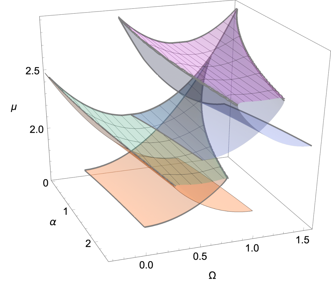
The spectrum consists in a set of surfaces which cross and merge at certain boundaries, as the ones plotted in Fig. 1 and their symmetric versions at . Five sections of with constant are plotted in Fig. 2. Except for the ground state at , they present a set of concatenated swallowtail (ST) shapes. For any given , each series of swallowtail diagrams represents a set of stationary solutions continuously connected among them through the parameters and , or through the velocity and chemical potential . These type of energy diagrams are characteristic of hysteresis and were analyzed in the context of ring condensates in mueller02. We organize and label them, and the surfaces that they constitute, according to their position, ordered from lower to higher energy. For each diagram we distinguish a bottom and a top part, both merging at the tip of the swallowtail. In the following we present their general features. The structure of the spectrum is analyzed more thoroughly in App. B.
Each energy level —top or bottom part of a swallowtail diagram— is symmetric with respect to and bounded by a pair of critical velocities , with an integer. Solutions corresponding to a level centered at a link velocity , are a boost from those in the analogous level at or . The th set of swallowtail diagrams, being the bottom one, entails densities with depressions, considering both the valleys characteristic of the Jacobi functions, and the downward kinks in the case of . We distinguish three types of solutions, depending on the depth of the depressions: vortex states, dark solitons, and gray solitons.
Vortex states. The red parabolas of plot (c) () in Fig. 2 centered at represent the chemical potential of vortex states of angular momentum as observed from the frame moving at . The minima of are at , where the observer is comoving with the vortex.
Dark solitons. At precisely , solutions consist in dark solitonic trains (except for the ground state), see the black dots in Fig. 2. In the delta comoving frame, the dark solitonic trains are stationary, with zero current and constant phase, except for a phase jump of at each zero in the density. They correspond to the minima of the energy spectrum for any particular fixed . In the lab frame, they comove with the condensate and the delta link at .
Gray solitons. Solutions with velocities that depart from , consist in gray solitonic trains, with shallower waves and faster currents the larger . At , gray solitonic trains with depressions become completely flat and merge with vortex states at , with
| (7) |
see App. B or carr002. At , the rotational symmetry is broken, and a pair of critical velocities, corresponding to the tips of the swallowtails, limit the range of for which stationary solutions exist. In particular, the width of the bottom part of the th swallowtail centered at monotonously decreases from , at , to at . The condensate in the ring is therefore able to sustain stationary solutions, consisting in gray solitonic trains comoving with the kink, up to a certain stirring velocity —relative to —, which decreases with the strength of the delta link.
A sample density and phase for each colored region of Fig. 1 (and the corresponding ones at ), are plotted in Fig. 3. The densities corresponding to the bottom of first swallowtail surface at entail an upward kink. This kink becomes higher and more peaked as the delta potential becomes more attractive, and can be understood as a bright soliton. In contrast, for the rest of levels, as , the density at the delta position becomes zero. The densities corresponding to the first swallowtail diagram have one depression, which for consists of one valley and for a downward kink. Similarly, the four plots corresponding to the second swallowtail levels have two depressions. For , one of these depressions is also understood as the downward kink imposed by the delta. From these plots it can also be inferred the relation between the the phase and the density, , which implies higher phase gradients (velocities) for lower densities.
III.2 Metastability
A Dirac delta with fixed strength and rotating at a constant speed allows an infinite set of solutions organized in chemical potential levels. The stability of these solutions can be studied by adding a small perturbation to the stationary wave function
| (8) |
and analyzing how it evolves. Replacing this function in the time-dependent Gross-Pitaevskii equation (Eq. (23)) and linearizing in and , we obtain the corresponding Bogoliubov system of equations bogoliubov47,
| (9) | |||
| (10) |
Both perturbations, and , must satisfy the boundary conditions separately, which read,
| (11) | ||||
| (12) | ||||
| (13) | ||||
| (14) |
We solve this system of equations, by changing variables to
| (15) | |||
| (16) |
and then expanding and in an orthonormal basis, thus converting it into a matrix eigenvalue problem, and by the Direct and Arnoldi methods integrated in the differential solvers in Mathematica, see App. E for more details.
Both methods yield the same eigenvalues, and analyzing whether they are real or complex, we split each region in stable and unstable parts.
The bottom of the first swallowtail and both upper parts are found completely stable and unstable, respectively. In contrast, the lower part of the second swallowtail is stable except for regions of metastability in form of stripes in the plane at , as shown in Fig. 4.
III.3 Dependence on nonlinearity

The results presented in the previous subsections have been illustrated with the nonlinearity fixed to . In Fig. 5 we show the same adiabatic regions for , and . The first and third columns correspond to the bottom part of first and second swallowtail diagrams (as in Fig. 2), while the middle column represents the top part of the first one. Larger nonlinearity implies a greater span and overlap of all the levels. As decreases, and for any fixed , the tail part of the swallowtail diagrams becomes smaller, vanishing at : both the region in the middle column and the overlaps of shifted regions in the others decrease in size. A condensate with larger nonlinearity is therefore able to sustain stationary solutions for faster stirring velocities, while in the linear limit, , the critical velocities are independent of the delta strength and fixed to .
Performing the same metastability analysis we find that the bottom part of the first swallowtail and both upper parts remain completely stable and unstable for all the tested. The third region of Fig. 5, corresponding to the bottom of the second swallowtail diagram, is also found completely stable at , while the metastable stripes at become thiner (thicker) as decreases (increases).
IV Adiabatic generation of vortex states and excited solitons

All complex solutions found are continuously connected at , where gray solitonic trains merge into vortex states as their velocity departs from , with an integer (see middle panel of Fig. 2). Once a finite delta strength is set, a gap between the various swallowtail diagrams appears, and depending on the initial rotational velocity and initial state, different energy levels can be accessed. In particular, setting a delta link in the ground state while rotating at , , a gray solitonic train with depressions is obtained—reaching thus the bottom of the th swallowtail diagram. As the velocity is decreased, the valleys become deeper, and at the solution turns into a wave train with dark solitons. If the velocity is further decreased, the density profile becomes a gray solitonic train again, with shallower waves with lower velocity. At any velocity, one can unset the delta link, making the waves shallower as the delta strength decreases back to . For , unsetting the link completely flattens the density, and the ground state is recovered. At velocities , the final state consists in a gray solitonic train, with deeper waves the closer is to . If one unsets the delta link at precisely , a dark solitonic train is obtained. In the case in which is brought back to zero at , the waves also become infinitely shallow, and merge with the vortex state of quanta.
Cycles in which the final state is a vortex can be concatenated. Once a vortex is produced, any observer can rotate at the same velocity as the condensate current, such that in the comoving frame the vortex is observed as the ground state. The cycle to produce a vortex from the ground state can then be repeated. Let us consider the vortex state of five quanta of angular momenta. It can be produced by setting a delta link rotating at , decreasing its velocity to , and then unsetting the delta. It involves a middle step in which a wave train with five dark solitons is produced. Another possibility is to concatenate five analogous cycles in which , and , each involving the production of only one dark soliton. After each individual cycle, the observer is boosted .
Any of these proposed paths should avoid the metastable and non-stationary regions analyzed in the previous section. In Fig. 6, we schematically demonstrate four of such adiabatic paths. They excite the condensate to one dark soliton and a vortex state, each one through the setting and unsetting of a delta link, either repulsive or attractive. In both cases, the delta strength is limited by the line bounding the adiabatic region corresponding to the bottom of the second swallowtail. For the attractive delta, one also needs to avoid the metastable region, which further limits the value of . These adiabatic cycles can be reproduced for all tested. However, the range of velocities at which the Dirac delta strength must be set, decreases with , . Moreover, in the case of the cycle with an attractive rotating delta, the constrain on the magnitude of the delta potential will depend on the metastability stripes shown in Fig. 5.
For any adiabatic path involving higher swallowtail levels, the corresponding metastability analysis and determination of critical velocity should be performed. Alternatively, one can simulate these cycles by solving the time-dependent Gross-Pitaevskii equation with the Dirac delta link replaced by a Gaussian one. We solve this differential equation using the method of lines, and reproduce the cycles proposed in Fig. 6. Moreover, we also obtain dark solitonic trains and vortex states with up to five solitons or quanta. On the one hand, these simulations validate the results found for the delta link. On the other, they indicate that the structure of the spectrum laid out in the delta case is also able to depict the main features of the spectrum of a BEC stirred with a peaked Gaussian link.
The velocities , constraining the adiabatic cycles, have been presented in natural units, where and . For a condensate of 87Rb atoms, with mass u and ring traps of radiuses to , the natural velocities range from rad/s to rad/s. Taking , the thresholds speeds to access the first excited states are , 2.95, 3.59 rad/s for the smaller radius, and , 0.118, 0.143 rad/s for the larger one. In the linear limit, , .
V Conclusions
The spectrum of a 1D ring condensate with a Dirac delta rotating at constant speed has been analyzed in terms of the nonlinearity , the delta velocity , and the delta strength . Analytical expressions are provided for the wave function, the current, and the chemical potential. For a fixed and , the dependence of the chemical potential on the delta velocity, , consists of a series of swallowtail diagrams. These diagrams can be organized from smaller to larger energies, and each one can be split into a bottom and a top part. The lowest diagram at is an exception, and consists only of the bottom part, with a more complex structure depending on a set of critical points . As the magnitude of the delta strength increases, the sizes of the tails in each diagram decrease, while the energy gap among each diagram becomes larger. At , the top parts of the diagrams merge with the bottom parts of the immediate upper ones. The spectrum thus consists in a multiple swallowtail 3D structure, each region providing a range of delta strengths and velocities which can be varied adiabatically to access different solitonic solutions. These solutions consist in gray or dark solitonic trains, where the number of depressions in each train has been related to the position of the swallowtail. In particular an odd (even) number of dark solitons comove with the condensate at , where is an odd (even) integer.
In order to support the possible adiabatic processes allowed by the Gross-Pitaevskii spectrum, we have analyzed the metastability of each solution for the first two swallowtail diagrams. The top parts are found unstable and the bottom ones stable, except for the bottom of the second diagram at , which presents a series of metastable stripes in parameter space.
We have proposed a method to produce dark and gray solitons, and vortex states of arbitrary quantized angular momentum, by controlling the stirring velocity and strength of the potential. The method consists in setting and unsetting a Dirac delta potential while rotating it around the condensate at certain velocities. In particular, as a rotating observer sets a delta link at , the bottom part of the th swallow tail is reached, and a gray solitonic train with depressions is produced. The cycles in the parameter space defined by and corresponding to the various production processes are constrained by the width of the swallowtail diagrams, and also by the metastable regions. These adiabatic paths are qualitatively reproduced by solving the time-dependent Gross-Pitaevskii equation in which a finite width Gaussian link is rotating at constant speed.
Appendix A Gross-Pitaevskii equation and boundary conditions
The evolution of the condensate wave function in the Lab frame, , is governed by the 1D Gross-Pitaevskii equation,
| (17) |
where is the atomic mass, the radius of the ring, and the angular and time coordinates in the lab frame, and the magnitude and angular velocity of the Dirac delta, and the reduced 1D coupling strength. The circular topology imposes continuity conditions in the wave function,
| (18) |
and the Dirac delta constrains its derivatives through boundary conditions. These are obtained by integrating Eq. (17) in a small contour around the delta, , and taking the limit ,
| (19) | ||||
We change variables to the delta rotating frame leggett73,
| (20) | ||||
| (21) | ||||
| (22) |
and use units . Then eqs. (17), (18), and (19) become,
| (23) | ||||
| (24) | ||||
| (25) |
For a stationary solution, , where is the chemical potential, these equations result in Eqs. (1)-(3).
Appendix B Solutions
To obtain the solutions of Eq. (1) we write the wave function as . Separating into real and imaginary parts, and integrating, the density and phase take the general form,
| (26) | ||||
| (27) |
where is one of the 12 Jacobi functions and , , , , , and are constants. The squares of the six convergent or divergent Jacobi functions are related among themselves linearly and through shifts in , and therefore one may consider only a convergent one and a divergent one with general , , and . Eq. (27) represents the stationarity condition, with the current. The shift is fixed by the continuity condition, : the angular length of the condensate, , has to be equal to an integer number of periods () plus twice the shift, (see Fig. 7).
The period of is given in terms of the elliptic integral of first kind (), , and therefore
| (28) |
Since we take and as a parameters, can be fixed to . Eqs. (1) and (4) fix , , and in terms of , , and . Using the Jacobi functions dn and dc as the convergent and divergent independent solutions, respectively, the amplitudes read,
| (29) | ||||
| (30) |
where
| (31) | ||||
| (32) |
with the elliptic integral of the second kind, the Jacobi amplitude, sc the Jacobi function, and where dc allows only for and in order to be convergent in . The phases and are then integrated from the Eq. (27).
For the types of Jacobi functions chosen, , the corresponding currents and chemical potentials read,
| (33) | ||||
| (34) |
This leaves the frequency and elliptic modulus as the only free parameters. They constrain and through the boundary conditions in Eqs. (2) and (3). and are either real, , , or, in the case of real solutions, may also take complex values with and . For the real solutions (with general real boundary conditions) we refer to perezobiol19. The elliptic modulus is further constrained by the condition that , which is satisfied when and odd number of radicants in Eq. 33 are positive. Note that the transition to an even number of radicants being negative, where is not real, happens at .
In the case of , the wave functions are plane waves, where , or solitonic trains, which have, for each level ,
| (35) |
Both expressions correspond to periodic boundary conditions (solved in Ref. carr002) and coincide at and . These values determine the critical velocity,
| (36) |
that bounds both regions and at .
For a similar treatment of the Jacobi functions and a complete derivation of the solutions see e.g. carr002. The main difference between carr002 and our work is that in carr002 and are not taken as parameters to account for a phase jump and a kink, but adjusted such that periodic boundary conditions are obtained.

Appendix C Computation of the spectrum
All solutions satisfying Eqs. (1)-(4) can be obtained by running and in their allowed ranges in any of the three Jacobi functions, two convergent and one divergent, and which we label as
| (37) | ||||
| (38) | ||||
| (39) |
Then, for each and , the delta strength, velocity, and the chemical potential are obtained from Eqs. (2), (3), and (1),
| (40) | ||||
| (41) | ||||
| (42) |
A sample of the spectrum produced this way is shown in plot (a) of Fig. 8. Its projection on the plane is potted on panel (b) of the same figure. In this plane, lines parametrized by and fixed , (,), and lines parametrized by and fixed , (,), are tangent at the degeneracy line,
| (43) |
see bottom-right panel of Fig. 8. Therefore, any degeneracy line may be computed by solving
| (44) |

Appendix D Spectral structure
Fig. 9 shows the projections of in the plane for the ground state and first excited levels. The ground and first excited state for present a more complex structure, which we analyze in this Appendix. Its bounds are determined by the limits of the elliptic modulus —0, 1, or the ones fixed by —, or by Eq. (44), and conform the set of lines uniting the points and . Each segment of these bounds is listed in Table 1 together with the function and limit of they represent. The line and its continuation at is the only curve not defining the degeneracy of two energy levels. The points , , themselves can be further determined. Points , , and correspond to and velocities , , and , respectively. The values of , are constrained by their current and elliptic modulus being zero, , while has and . Point is obtained by minimizing with . All these constrains fix to the values shown in Table 2.
| Region | Bounds | ||
| Bottom 1st ST | dn | , Eq. (44) | |
| , | |||
| dc | , | ||
| , | |||
| Bottom 1st ST | Eq. (44) | ||
| Top 1st ST | dn | , Eq. (44) | |
| , | |||
| Top 1st ST | Eq. (44) | ||
| Bottom 2nd ST | Eq. (44) | ||
| Bottom 2nd ST | dn | Eq. (44) | |
The dependence of the spectrum on can be analyzed quantitatively through the expressions in Table 2 for the points . , , , and are given in analytical form, and , , and are plotted in Fig. 10. approaches zero as increases, and the structures bounded by the lines and (middle panel in Fig. 9) vanish in the limit . In contrast, , and increase with , and the region bounded by these points grows at large interactions. At , where solves , both Eqs. for and in Table 2 are satisfied and points and coincide. In the limit , approaches at , and tend to zero, and : the parts of the region merge into a flat band. In general, at , all levels turn into regions spanning , where all the solutions are stable (see App. F for the linear solutions).
Appendix E Bogoliubov analysis
The differential equations and boundary conditions constraining and are
| (45) | ||||
| (46) | ||||
| (47) | ||||
| (48) | ||||
| (49) | ||||
| (50) |
In order to turn this system of equations into a linear eigenvalue problem, we expand and in an orthonormal basis. This basis does not consist in periodic plane waves, since the derivatives must be discontinuous according to the delta conditions, but in the solutions of Eqs. (1)-(4) with and . Imposing these constraints on exponential and trigonometric functions, we obtain the basis,
| (51) | ||||
| (52) | ||||
| (53) |
with a positive integer, and where the element is only used for . and expanded in this set of functions solve Eqs. (47) and (49), and Eqs. (48) and (50) are satisfied as long as and are the solutions of, respectively,
| (54) | ||||
| (55) |
Appendix F Linear limit
Solutions of Eqs. (1)-(4) with can be found analytically proceeding analogously to App. B and replacing Jacobi functions by trigonometric and hyperbolic ones. They read,
| (56) | ||||
| (57) |
where,
| (58) | ||||
| (59) | ||||
| (60) | ||||
| (61) |
and the frequency is real and the current positive. Note that and solutions are related by . For a given , is limited by the square roots in , being real. The phases, and , are computed according to Eqs. (27), (40), and (41), respectively, where now and are taken as parameters, and the chemical potentials read,
| (62) | ||||
| (63) |
The spectrum consists in a series of layered levels, each one spanning all and , given that , where etc., see Fig. 11. Adding a perturbation to these solutions in the form of Eq. (8) must satisfy the same linear equations with , as stated by Eqs. (9) and (10) with . The solutions only satisfy the boundary conditions for real eigenvalues, and therefore the frequencies are not imaginary and all the solutions stable.
Acknowledgments
This work was supported by the Japan Ministry of Education, Culture, Sports, Science and Technology under the Grant number 15K05216. We thank Muntsa Guilleumas, Bruno Juliá-Díaz and Ivan Morera for fruitful discussions and a careful reading of the paper. The article has also greatly benefited from ideas and comments from the Atomtronics 2019 community.
References
- (1) C. Ryu, M. F. Andersen, P. Cladé, V. Natarajan, K. Helmerson, and W. D. Phillips, Phys. Rev. Lett. 99, 260401 (2007).
- (2) S. Moulder, S. Beattie, R. P. Smith, N. Tammuz, and Z. Hadzibabic, Phys. Rev. A 86, 013629 (2012).
- (3) S. Beattie, S. Moulder, R. J. Fletcher, and Z. Hadzibabic, Phys. Rev. Lett. 110, 025301 (2013).
- (4) K. C. Wright, R. B. Blakestad, C. J. Lobb, W. D. Phillips, and G. K. Campbell Phys. Rev. A 88, 063633 (2013).
- (5) J. Dalibard, F. Gerbier, G. Juzeliūnas, and P. Öhberg, Rev. Mod. Phys. 83, 1523 (2011)
- (6) A. Ramanathan, K. C. Wright, S. R. Muniz, M. Zelan, W. T. Hill, C. J. Lobb, K. Helmerson, W. D. Phillips, and G. K. Campbell, Phys. Rev. Lett. 106, 130401 (2011).
- (7) F. Piazza, L. A. Collins, and A. Smerzi, Phys. Rev. A 80, 021601(R) (2009).
- (8) F. Piazza, L. A. Collins, and A. Smerzi, J. Phys. B: At. Mol. Opt. Phys. 46, 095302 (2013).
- (9) K. C. Wright, R. B. Blakestad, C. J. Lobb, W. D. Phillips, and G. K. Campbell, Phys. Rev. Lett. 110, 025302 (2013).
- (10) S. Eckel, J. G. Lee, F. Jendrzejewski, N. Murray, C. W. Clark, C. J. Lobb, W. D. Phillips, M. Edwards, and G. K. Campbell, Nature (London) 506, 200 (2014).
- (11) C. Ryu, P. W. Blackburn, A. A. Blinova, and M. G. Boshier, Phys. Rev. Lett. 111, 205301 (2013).
- (12) D. W. Hallwood, T. Ernst, and J. Brand, Phys. Rev. A 82, 063623 (2010); D. Solenov and D. Mozyrsky, Phys. Rev. A 82, 061601(R) (2010); A. Nunnenkamp, A. M. Rey, and K. Burnett, Phys. Rev. A 84, 053604 (2011); D. Solenov and D. Mozyrsky, J. Comput. Theor. Nanosci. 8, 481 (2011).
- (13) C. Schenke, A. Minguzzi, and F. W. J. Hekking, Phys. Rev. A 84, 053636 (2011).
- (14) L. Amico, D. Aghamalyan, F. Auksztol,H. Crepaz, R. Dumke, and L.-C. Kwek, Sci. Rep. 4, 4298 (2014).
- (15) R. Kanamoto, L. D. Carr, and M. Ueda Phys. Rev. A 79, 063616 (2009).
- (16) O. Fialko, M.-C. Delattre, J. Brand, and A. R. Kolovsky, Phys. Rev. Lett. 108, 250402 (2012).
- (17) Y. Li, W. Pang, and B. A. Malomed, Phys. Rev. A 86, 023832 (2012).
- (18) A. Muñoz Mateo, V. Delgado, M. Guilleumas, R. Mayol, and J. Brand, Phys. Rev. A 99, 023630 (2019).
- (19) S. Baharian and G. Baym, Phys. Rev. A 87, 013619 (2013).
- (20) A. Muñoz Mateo, A. Gallemí, M. Guilleumas, and R. Mayol, Phys. Rev. A 91, 063625 (2015).
- (21) M. Kunimi and Y. Kato, Phys. Rev. A 91, 053608 (2015).
- (22) L. D. Carr, C. W. Clark, and W. P. Reinhardt, Phys. Rev. A 62, 063610 (2000); Phys. Rev. A 62, 063611 (2000).
- (23) B. T. Seaman, L. D. Carr, and M. J. Holland, Phys. Rev. A 71, 033609 (2005).
- (24) V. Hakim, Phys. Rev. E 55, 2835 (1997).
- (25) N. Pavloff, Phys. Rev. A 66, 013610 (2002).
- (26) M. Cominotti, D. Rossini, M. Rizzi, F. Hekking, and A. Minguzzi, Phys. Rev. Lett. 113, 025301 (2014).
- (27) E. J. Mueller, Phys. Rev. A 66, 063603 (2002).
- (28) N. Bogoliubov J. Phys. USSR 11, 23-32 (1947).
- (29) A. J. Leggett, Phys. Fenn. 8, 125 (1973).
- (30) A. Pérez-Obiol and T. Cheon, J. Phys. Soc. Jpn. 88, 034005 (2019).