Localization of gauge bosons and the Higgs mechanism on topological solitons in higher dimensions Preprint: YGHP-19-02
Abstract
We provide complete and self-contained formulas about localization of massless/massive Abelian gauge fields on topological solitons in generic dimensions via a field dependent gauge kinetic term. The localization takes place when a stabilizer (a scalar field) is condensed in the topological soliton. We show that the localized gauge bosons are massless when the stabilizer is neutral. On the other hand, they become massive for the charged stabilizer as a consequence of interplay between the localization mechanism and the Higgs mechanism. For concreteness, we give two examples in six dimensions. The one is domain wall intersections and the other is an axially symmetric soliton background.
I Introduction
The idea that our world is a four-dimensional hyper surface (a 3-brane) in higher-dimensional spacetime has been widely studied for decades. Such models are called brane-world models. By utilizing geometry of the extra dimensions, the brane-world models can solve many unsatisfactory problems of the Standard Model (SM), as provided by the seminal works ArkaniHamed:1998rs; Antoniadis:1998ig; Randall:1999ee; Randall:1999vf.
A conventional setup of the brane-world models is that extra dimensions are prepared as a compact manifold/orbifold. Namely, our four-dimensional spacetime is treated differently from the extra dimensions. Furthermore, 3-branes are introduced by hand as non-dynamical objects which are infinitely thin. In order to make the models more natural, we can harness topology of extra dimensions. The idea is quite simple Rubakov:1983bb: Dynamical compactification of the extra dimensions and dynamical creation of 3-branes originate in a spontaneous symmetry breaking in a vacuum. Namely, it gives rise to a topologically stable soliton/defect of a finite width. The topology ensures not only stability of the brane but also the presence of chiral matters localized on the brane Jackiw:1975fn; Rubakov:1983bb. In addition, graviton can be trapped Cvetic:1992bf; DeWolfe:1999cp; Csaki:2000fc; Eto:2002ns; Eto:2003bn; Eto:2003ut.
In contrast, localizing massless gauge bosons, especially non-Abelian gauge bosons, is quite difficult. There were many works so far Dvali:2000rx; Kehagias:2000au; Dubovsky:2001pe; Ghoroku:2001zu; Akhmedov:2001ny; Kogan:2001wp; Abe:2002rj; Laine:2002rh; Maru:2003mx; Batell:2006dp; Guerrero:2009ac; Cruz:2010zz; Chumbes:2011zt; Germani:2011cv; Delsate:2011aa; Cruz:2012kd; Herrera-Aguilar:2014oua; Zhao:2014gka; Vaquera-Araujo:2014tia; Alencar:2014moa; Alencar:2015awa; Alencar:2015oka; Alencar:2015rtc; Alencar:2017dqb. However, each of these has some advantages/disadvantages and there seems to be only little universal understanding. Then a new mechanism utilizing a field dependent gauge kinetic term (field dependent permeability)
| (1) |
came out in Ref. Ohta:2010fu where are scalar fields which we call stabilizer throughout this paper. This is a semi-classical realization of the confining phase ArkaniHamed:1998rs; Dvali:1996xe; Kogut:1974sn; Fukuda:1977wj; Luty:2002hj; Fukuda:2009zz; Fukuda:2008mz. Recently, one of the author and the collaborators have tried to improve the brane-world models with topological solitons by using (1) Arai:2012cx; Arai:2013mwa; Arai:2014hda; Arai:2016jij; Arai:2017lfv; Arai:2017ntb; Arai:2018rwf; Arai:2018uoy; Arai:2018hao. Brief highlights of the results are the following: Ref. Arai:2017ntb provided the geometric Higgs mechanism which is the conventional Higgs mechanism driven by the positions of multiple domain walls in an extra dimension, similarly to D-branes in superstring theories. Then the geometric Higgs mechanism was applied to Grand Unified Theory in Ref. Arai:2017lfv. However, in these early works, treatment of gauge fixing was partially unsatisfactory. In order to resolve this point, we have developed analysis by extending the gauge under spatially modulated backgrounds in any spacetime dimensions Arai:2018rwf. Then, we gave a new attempt in Ref.Arai:2018uoy that the SM Higgs field plays a role of the stabilizer in a model. The latest development along this direction is that the same localization mechanism can be applied not only on vector fields but also scalars and tensors in Ref. Arai:2018hao. Another group also recently studied the SM in a similar model with taken as a given background in Okada:2017omx; Okada:2018von; Okada:2019fgm.
The purpose of this paper is to provide complete and self-contained formula about localization of massless/massive Abelian gauge fields on topological solitons in generic dimensions via the field dependent gauge kinetic term (1). The basic template is a domain wall in a model with stabilizers which are neutral to the would-be localized gauge fields. Such models have been studied in Ref. Ohta:2010fu; Arai:2012cx; Arai:2013mwa; Arai:2014hda; Arai:2016jij; Arai:2017lfv; Arai:2017ntb. We firstly reanalyze it with the extended gauge to provide more complete arguments in Sec. II. Then, there are two directions for extending the basic template. The one is to go to higher dimensions , and the other is to make the neutral stabilizers charged to the would-be localized gauge fields. The former direction has been investigated in Ref.Arai:2018rwf which we will give a review with several improvements especially on divergence-free parts of extra-dimensional components of the gauge fields in Sec. III. The latter extension that localization of gauge fields by charged stabilizers was applied to the SM in dimensions Arai:2018uoy. In Ref. Arai:2018uoy, the charged stabilizer is nothing but the SM Higgs field. Therefore, the Higgs field plays three roles: breaking of the electroweak symmetry, generating fermion masses, and localizing the electroweak gauge bosons on the domain wall. Since details on gauge field localization by the charged stabilizer were not given in Ref. Arai:2018uoy, in this work we will give a complete formula in details for accounting localization mechanism which occurs together with the Higgs mechanism in Sec. IV. Finally, we proceed to unify the two directions into the most generic models in with charged stabilizers. In general, fluctuations are mixed each other under a soliton background, so that it is not easy to distinguish which field is physical or unphysical. To overcome this difficulty, we will carefully analyze the small fluctuations in the extended gauge in Sec. V, and succeed in cleaning up related Lagrangian up to quadratic order of the fluctuations, and providing a simple and compact formula. With the formula at hand, it becomes easy for us to obtain physical mass spectra appearing in a low energy effective theory on topological solitons for generic models. To be concrete, we give examples in Sec. VI. The first example is an intersection of two normal domain walls in dimensions. We will find an extremely good approximation which allow us to compute analytically mass spectra localized on an intersecting point. In the second example, we take an axially symmetric background on the assumption that the topological soliton is a vortex-type soliton in .
For both cases that the stabilizer is neutral and/or charged, our formula provides us a transparent road to obtain the physical mass spectra, and to specify the lightest degrees of freedom in the low energy effective theory. We will figure out that the lightest fields are massless four-dimensional gauge bosons and Nambu-Goldstone fields for the neutral stabilizer. There are infinite tower of Kaluza-Klein (KK) modes but there is a large mass gap (of order inverse soliton width) between the low-lying mode and the higher KK modes. Once we replace the neutral stabilizer by charged one, the Higgs mechanism occurs together with localization of the gauge fields. As a result, the lowest mass mode becomes the massive four-dimensional gauge field, and the heavy KK modes follow with the large mass gap. We should stress that the scalar fields originated from the extra-dimensional components of the gauge fields are always above the large mass gap, so that they do not supply any low-lying physical degrees of freedom.
The organization on the paper is the following. The basic template of the localization mechanism with neutral stabilizers in is given in Sec. II. The extension of Sec. II with the neutral stabilizers in higher dimensions is explained in Sec. III. Sec. IV is devoted to explain the other generalization of Sec. II with charged stabilizers in . Then, the most generic models with charged stabilizers in higher dimensions is studied in Sec. V. Several concrete examples in are given in Sec. VI, and concluding remarks are given in Sec. VII.
II Localization by a neutral stabilizer in
II.1 The model
We consider the following Lagrangian in non-compact five dimensions,
| (2) | ||||
| (3) |
where , and is a complex scalar field, is a real scalar field, and is a gauge field. The field strength is given by
| (4) |
For to be real, should be a real functional of . The scalar Lagrangian depends on and as
| (5) |
As we will see below, is responsible for generating a non-trivial soliton background configuration, and plays an important role for localizing gauge fields on the soliton. We will refer to as a stabilizer. In this section, we will also assume that both and are neutral under the gauge transformation associated with the gauge field ; Namely, they do not interact with the gauge field through conventional covariant derivatives. Nevertheless, the neutral stabilizer can couple to through the factor in front of the term. Clearly, if is a constant, the Lagrangian reduces to a conventional minimal one. Note that can be interpreted as an extension of inverse square of a gauge coupling constant which can be a function of the stabilizer .
The Euler-Lagrange equations of the model read
| (6) | |||
| (7) | |||
| (8) |
Clearly, solves the last equation. Then, we are left with the first two equations with zeros at the right hand sides. Hereafter, we will assume that and take a nontrivial background configuration depending only on the extra-dimensional coordinate . Such configurations generically appear as a topological soliton when a discrete symmetry is spontaneously broken.
II.2 An illustrative example
Before describing a generic model, let us make a pause for illustrating relevant phenomena through one of the simplest example in . Let us consider the scalar potential
| (9) |
The model has the global symmetry , and the symmetry . When , there are two discrete vacua . Thus, the symmetry is spontaneously broken, which gives rise to a topologically stable domain wall: It is straightforward to verify that the analytic domain wall solution is given by
| (10) |
where and are real moduli parameters, and we defined . The symmetry is recovered at the center of domain wall , whereas the unbroken symmetries at the vacua, namely the translational symmetry and the global symmetry, are spontaneously broken only near the domain wall. This locally broken symmetries are responsible for the presence of the moduli parameters under the Nambu-Goldstone theorem. Another domain wall solution is known for as
| (11) |
Here, the global symmetry is unbroken everywhere. Thus, there is only the translational moduli parameter .
Either the translational symmetry or the global symmetry is broken in the vicinity of the domain wall whereas they are not broken at the vacua. Therefore, we expect the corresponding zero modes are localized on the domain wall. This can easily be verified by perturbing the background solution as
where , , and are real. In the following, we will set just for ease of the notation. Plugging these into the Lagrangian and taking the terms quadratic in the fluctuations (we will shortly take fluctuations of the gauge fields into account below), we find
where we defined
and
The KK mass spectra for can be obtained by expanding by eigenstate of as
| (26) |
Now, it is clear that there always exists the translational zero mode:
As expected, this is localized around the domain wall, which can easily be verified by looking at . Note that the translational zero mode exists regardless of values of the parameters .

We can also derive several exact results for massive modes. Analysis for is easy since is diagonal. There are two orthogonal low lying mass eigenstates
is monotonically increasing function of whereas the degenerate masses are monotonically decreasing function. The two masses cross at , see Fig. 1. The thresholds (the dotted lines in Fig. 1) between localized discrete modes and scattering continuum modes are and for and , respectively. At the critical point , becomes exactly massless, whereas becomes heavy whose mass is of order . There, the quadratic Lagrangian switches from the upper to the lower one in Eq. (II.2). It is not easy to analytically compute mass eigenvalues for ,11 1 The negative mass square implies that is unstable for . Indeed, for the solution in Eq. (10). since is no longer diagonal. However, due to the continuity at , and should continuously be connected to corresponding degrees of freedom for . Let us estimate the eigenvalues by treating as a small perturbation. To the first order of defined by
| (36) |
the mass eigenvalues are calculated as
| (37) | |||||
| (38) |
Thus, the both eigenvalues grow up as increasing, see the yellow band in Fig. 1.
On the other hand, a linear combination of remains massless, and transforms to the NG mode. Indeed, never vanishes at finite for , so that has the non minimal kinetic term. To make the lower Lagrangian of Eq. (II.2) be canonical, let us redefine by
| (39) |
Then, the quadratic Lagrangian can be rewritten as
| (40) |
with
| (41) |
The mass spectrum corresponds to the eigenvalues of the Hermitian operator as
| (42) |
Since is positive semidefinite, the eigenvalues are . The normalizable zero mode is uniquely given by
| (43) |
There are no other localized modes. All the excited states are continuum modes and given by
| (44) |
Thus, the mass gap between the zero mode (the NG mode ) and the continuum scattering modes is .
The final piece of the fluctuation analysis is on the gauge fields. Since the background gauge fields are zeros, let itself be fluctuations. A relevant part to quadratic order in the fluctuation is
| (45) |
To illustrate essence, let us take one of the simplest example
| (46) |
where is a constant for . Since nothing interests happen for , we will investigate the parameter region in what follows. To figure out mass spectrum of the gauge field, we first need to fix the gauge symmetry. To this end, we add the following to the quadratic Lagrangian
| (47) |
Here, is a gauge fixing parameter. If is a constant, it reduces to a conventional covariant gauge . We call Eq. (47) the extended gauge Arai:2018rwf; Arai:2018uoy; Arai:2018hao; Okada:2017omx; Okada:2018von; Okada:2019fgm. In terms of the canonically normalized gauge field defined by
| (48) |
the quadratic Lagrangian reads
| (49) | |||||
Thanks to the gauge fixing term in Eq. (47), and are not mixed. Hence, the KK mass spectra of and correspond to eigenvalues of and , respectively. It is coincident for the particular choice of in Eq. (46) that the Schrödinger operators for and are identical (As we will see below, they are different in generic models.). Therefore, the KK mass spectrum of consists of for the localized mode and for the continuum scattering states with the momentum . Fortunately, no further computations are needed for , since and operators have the same mass eigenvalues except for a zero eigenvalue. Therefore, the mass square for is given by . It is peculiar that they depend on the gauge fixing parameter . Since any observable should not depend on gauge, we conclude that do not include any unphysical degrees of freedom. As we will show below, one can understand they are eaten by to give longitudinal modes of the massive KK modes of .
II.3 Generic models
So far, we have argued over the specific model with the scalar potential (9) and linear in given in Eq. (46). For a generic scalar potential, the matrix given in Eq. (II.2) is modified as
Accordingly, the detail mass spectrum of the scalar fields are different from those for the simplest model considered above. However, the presence of the translational NG mode is intact, and indeed the mode function given in Eq. (II.2) formally remains correct. Furthermore, the quadratic Lagrangian of the scalar sector given in Eq. (40) is also formally valid for the generic model. Therefore, we again have the following for
| (53) |
Here, although the profile itself is different from Eq. (10) in general, but the definition of the operators and are same as Eq. (41).
On the other hand, the gauge sector given in Eq. (49) gets modified when we generalize the linear function to a generic function . After a little computations, we get
| (54) | |||||
Compared to Eq. (49), and are replaced by and which are defined by
| (55) |
Note that and hold when is linear in .
To complete the analysis, let us expand and by eigenfunctions of and , respectively. To this end, let us introduce the eigenfunctions
| (56) |
Similarly to , is positive semidefinite, so that . The normalizable zero mode, if it exists, is unique. It is given by
| (57) |
Hereafter, we assume that is non zero and square integrable
| (58) |
We expand in terms of as
| (59) |
Thus, we conclude that always has the unique normalizable massless mode .
Similarly, we expand by the eigenfunctions of
| (60) |
As , holds. The massless eigenfunction is given by
| (61) |
However, this is non normalizable since we always impose the square integrability condition (58). As is well-known, for the massive modes with , we have the following relations
| (62) |
Thus, is expanded as
| (63) |
Plugging these into Eq. (54) and integrating it over , we find the quadratic Lagrangian for the low energy effective theory
| (64) |
with
| (65) | |||||
| (66) |
Clearly, is a usual Lagrangian in the gauge (covariant gauge) for the massless Abelian gauge field in four dimensions. Similarly, is identical to a conventional Lagrangian in the gauge for the Abelian gauge field which gets the mass as a result of the Higgs mechanism by absorbing the scalar field . Thus, does not provide any physical degrees of freedom to the low energy effective action but is converted into longitudinal degrees of freedom to .
Before closing this section, for later convenience, let us describe the above results from a slightly different view point. We decompose into a divergence part and a divergence-free part as
| (67) |
where the separation is done by the following projection operator
| (68) |
Then, it holds
| (69) |
Furthermore, we can easily show is orthogonal to the zero mode of as
| (70) |
This ensures that the projection operator is well-defined. Now, we can rewrite the quadratic Lagrangian of the gauge sector given in Eq. (54) as
| (71) | |||||
Note that the divergence-free condition (69) implies
| (72) |
with being a constant in . Indeed, this corresponds to the non-normalizable zero mode of given in Eq. (61). Therefore, eliminating from in Eq. (63) is nothing but getting rid of the divergence-free part form . Thus, eliminating the unphysical , the quadratic Lagrangian reduces to
| (73) | |||||
where we defined
| (74) |
Now, we run into a direct correspondence between the mass square operators for and for . This implies is the one which is eaten by . Thus, our statement becomes more solid than before: The divergence-free part of is unphysical because it diverges at the spatial infinity. The divergence part of is also unphysical because it is absorbed by .
Since is orthogonal to , is also orthogonal to . Thus, we can expand by the eigenfunction of as
| (75) |
This is perfectly consistent with Eqs. (63) and (74). Comparing this with the decomposition of in Eq. (59), it is quite natural that the absorbing state and the absorbed state have the same wave function .
We briefly summarize the gauge sector with Fig. 2. There are only two massless states in the low energy effective theory in four dimensions: the one is the gauge field and the other is the NG field . There are infinite KK towers of (eating ), and . Several lower KK discrete modes would be localized on the domain wall, followed by the infinite KK bulk modes. These spectra are dependent of the details of the model. However, it is always true that the massless states are gapped from the KK towers by the order of inverse of the domain wall width.

III Neutral stabilizers in higher dimensions
Let us next extend the previous models to generic dimensional models. We study the Lagrangians which are formally same as those given in Eqs. (2) and (3), by reinterpreting the spacetime indices . In the following arguments, we will not specify a concrete model for the scalar part , as we did in Sec. II.3. Instead, we will assume that the Lagrangian allows for the scalar field to give rise to a topological soliton whose world-volume dimensions are four (codimension is ). For example, a domain wall in , a vortex in , a monopole in , and so on.22 2 Here, symbolically stands for multiple scalar fields which are needed to form a topological soliton. Furthermore, we will assume that the neutral stabilizer locally condenses about the topological soliton as
Hereafter, we will use to express the extra dimensional coordinates . Thus, the coefficient in the gauge kinetic term (3) becomes a nontrivial function of the extra dimensional coordinates as
| (79) |
As a natural extension of Eq. (58), it will turn out that the sufficient condition to for a massless gauge field to be localized on the topological soliton is the square integrability of
| (80) |
This implies that is non-zero and quickly approaches to zero at the extra-dimensional spatial infinity.
III.1 Useful formulae
For later convenience, let us first correct some useful equations. Let us introduce a differential operator and its adjoint operator by
| (81) |
Clearly, these are natural extensions of and given in Eq. (55). They satisfies the following algebra
| (82) |
We will frequently encounter a self-adjoint operator defined by
| (83) |
where the sum on is implicitly taken. We will also use the following vector notation
Clearly, is positive semidefinite. Let be eigenstates of as
| (88) |
Suppose be a normalizable eigenfunction. Then, we have
| (89) |
Therefore, must be annihilated by all ’s as
| (90) |
There is a unique solution up to a normalization constant to these equations
| (91) |
We now understand the square integrability condition (80) is nothing but ensuring the normalizablity for the zero mode of . Namely, we here proved the existence and uniqueness of the normalizable zero eigenfunction of . Note that the previous work Arai:2018rwf also studied the zero mode , where the uniqueness was only proved for a radially symmetric background solution which is a function of .
Another self-adjoint operator will also take part in the following arguments,
| (92) |
Similarly to , this operator is positive semidefinite. An obvious zero eigenstate is given by
| (93) |
up to a constant. However, this is non-normalizable under the condition (80). Thus, we conclude that there are no normalizable eigenstates for zero eigenvalue of .
There is a useful corollary. Let be a set of non-singular and finite functions. Then we find that is orthonormal to . This can be shown as follows:
| (94) |
where we have used Eq. (90).
Finally, let us mention about which is “super-partner” of . Note that is a matrix operator and it is different form the one by one operator . Zero eigenstates of are given by
| (95) |
with being a constant vector. This is non-normalizable under the condition (80). It is easy to show that non-zero eigenvalues of and coincide as
| (96) |
III.2 The quadratic Lagrangian
With these preparations at hand, we are now ready to study mass spectra of the small fluctuations about the soliton background. We use the same notations for the scalar fluctuations , and as Eq. (II.2). Of course, here, we understand to represent the extradimensional coordinates . As in the five dimensional case, for the soliton background, and we again use itself for the small fluctuations.
First thing we have to do is to fix the gauge symmetry. To this end, similarly to the case, we add the following gauge fixing term
| (97) |
As before, we use canonically normalized fields . Then, we find that the quadratic Lagrangian consists of two independent parts: The scalar part and the gauge part as
| (98) |
The gauge part is given by
| (99) |
with
| (100) | |||||
| (101) |
We defined
| (102) |
which satisfies the following identity
| (103) |
The scalar part for is given by
| (104) |
with
III.2.1 The scalar part
We can further rewrite the above scalar quadratic Lagrangian with respect to the canonically normalized field defined in Eq. (39) as
| (110) |
where we defined the differential operators which are natural extension of and by
| (111) |
As in the five dimensional model, and coincide if . It is obvious that has a unique zero eigenstate
| (112) |
Thus we conclude that has the physical zero mode ( NG mode) and expanded as
| (113) |
III.2.2 The four dimensional component
The quadratic Lagrangian for
| (114) |
is a natural extension of Eq. (54) by exchanging by . We naturally expand the four dimensional components by the eigenfunctions of as
| (115) |
As was proved in Eq. (91), the ground state is unique with , and there is a finite mass gap (about inverse of the background soliton width) between the ground state and excited states. Plugging this into the Lagrangian and integrating it in the extra dimensional coordinate , we find the four dimensional effective Lagrangian for as
| (116) |
III.2.3 The extra dimensional component
Let us next turn to the extra dimensional components which provide additional scalar fields to the low energy effective theory in four dimensions. The multiple scalars make the quadratic Lagrangian more complicated compared to the one in five dimensions. To make the matter clear, let us first decompose into a divergence part and divergence-free parts as
| (117) |
with a projection operator
| (118) |
It satisfies the following equations
| (119) |
With these at hand, it is straightforward to verify the divergence free condition should be satisfied
| (120) |
One immediately finds that includes a component proportional to as
| (121) |
with being an arbitrary but constant vector, and standing for rest component orthogonal to . However, we should remove since it diverges at the spatial infinity. This is an extension of Eq. (72) in the case. In contrast to the case, there still exist physical degrees of freedom in in the higher dimensions. From the definition of given in Eq. (117) and the identity (103), it also follows
| (122) |
Since the projection operator includes the inverse of , one might worry whether it is well defined or not. However, it is always well defined because is orthonormal to the zero mode of , see the corollary in Eq. (94).
Now, by using Eqs. (120) and (122), we can rewrite the quadratic Lagrangian as
| (123) |
The divergence and the divergence-free parts are decoupled.
The divergence part
Let us first examine the divergence part. The divergence part essentially include only one independent degree of freedom. Similarly to the five dimensional case in Eq. (74), let us define a scalar field as
| (124) |
Then, the divergence part of Eq. (123) can be written as
| (125) |
Since is orthogonal to the zero mode of , is also independent of . Hence, is expanded by the eigenstates of as
| (126) |
Then contributions to the low energy effective action from the divergence part is
| (127) |
This together with Eq. (116) for the four dimensional component , we confirm that the massless gauge boson robustly exists even in higher dimensional case, and all the KK modes become heavy by eating .
The divergence-free parts
Our last task in this subsection is clarifying mass spectra for the divergence-free part , which are new degrees of freedom appearing only for . To this end, let us first note that the operator can be expressed in the following form
| (128) |
where is an dimensional completely anti-symmetric tensor. We can rewrite this as a product of a matrix and its adjoint as
| (129) |
One can easily imagine the components of from the first several examples
| (130) | |||||
| (131) | |||||
| (132) |
We can construct from as
where means whose indices are all shifted by 1 as . Obviously, the decomposition is not unique under a unitary transformation with . However, this ambiguity does not yields any physical consequences. So we fix the ambiguity by choosing a specific . We are primally interested in existence of a massless state since its presence would be critical in the low energy effective theory on the host topological soliton.
Since in Eq. (129) is semi-positive definite, the zero eigenstate is unique and satisfies
| (141) |
For example, this condition in the cases read
| (142) | |||||
| (143) | |||||
| (144) |
These can easily be generalized in generic dimensions as
| (145) |
for all . By using the definition in Eq. (81) and the assumptions , we can rewrite this as
| (146) |
Let us take any three indices from , say . For this choice, is just a vorticity zero condition to the three vector . The same is true for any choice of three indices. Therefore, from the conventional Stokes’ theorem in three spatial dimensions, the massless condition (146) means that there exists a potential by which any can be expressed as
| (147) |
Finally, we have to verify if this is divergence-free or not. Indeed, it is a divergence part which can be seen as
| (148) |
Namely, the operator has no divergence-free zero modes in generic dimensions.33 3 We should mention about the result of the previous work Arai:2018rwf on the divergence free part. In Arai:2018rwf, the spectrum of the divergence free parts was studied only for case in detail where the absence of the massless mode was assumed. Furthermore, the massless modes in higher dimensional models () were not understood very well in Arai:2018rwf.
In order to clarify massive modes of the divergence-free parts, firstly, let us introduce the eigenvectors and eigenvalues of the Hermitian operator dual to as
| (149) |
where is a vector whose component is (). Then it is straightforward to show
| (150) |
A nice thing for this is that the divergence-free condition is automatically satisfied for any as
| (151) |
This can be proved by acting on given in Eqs. (142) – (144) as
| (152) |
Expanding the divergence-free parts as
| (153) |
and plugging this into the quadratic Lagrangian and integrating it over the extra dimensions, we get
| (154) |
This expression is formally valid for any .
Unfortunately, it is still not clear the relation between the eigenvalue of the operator and of the operator. For this point, the case is especially simple as
| (155) |

We briefly summarize the gauge sector with Fig. 3. Similarly to the 5 case, there are only two massless states in the low energy effective theory in four dimensions: the one is the gauge field and the other is the NG field . In addition to the infinite KK towers of (eating ), , there newly appear another KK towers of .
IV Localization by a charged stabilizer in
In this section, we will again consider five dimensional models in which the stabilizer is not neutral but has a charge to the would-be localized gauge field. Namely, we slightly modify the Lagrangian in Eq. (5) as
| (156) |
with the conventional covariant derivative
| (157) |
As before, we adopt the notation that the gauge coupling constant is absorbed in the gauge field , and stands for a charge of to the gauge transformation. Except for the change , we will not modify the Lagrangian (2). Thus, the Lagrangian respects the five dimensional Lorentz symmetry and the gauge symmetry. The charged stabilizer now interacts with the gauge field through both the covariant derivative and the function in front of the term. This is a seed for a mixture of the Higgs mechanism which takes place inhomogeneously, and the localization of the gauge field on the domain wall. This is what we will clarify in this section.
The Euler-Lagrange equations are slightly modified as
| (158) | |||
| (159) | |||
| (160) |
Note that we can set to be real, and then solves the third equation. The first and second equations with are identical with those in the previous section, so that the background soliton configuration with and ( is real) remains as the solution. In what follows, we will assume .
Let us next perturb the background solution as before. The fluctuations are introduced as , , and itself stands for the small fluctuation. We will obtain a quadratic Lagrangian for the fluctuations for figuring out mass spectra. A difference from the previous model with the neutral scalar resides only in the covariant derivative as
| (161) |
Namely, a change from the neutral scalar case is realized by just an exchange
| (162) |
Therefore, the quadratic Lagrangian of the scalar sector can immediately obtained as
| (163) |
where , and and are defined in Eqs. (II.2) and (II.3), respectively. Let us rewrite the quadratic Lagrangian with respect to the canonical field defined in Eq. (39) as
| (164) | |||||
Comparing this to Eq. (40) for the neutral case, the terms with are added. On the contrary, the gauge sector is unchanged since it is independent of . However, the scalar sector newly include the mixing terms between and which we would like to eliminate to diagonalize mass matrices. To this end, we need to modify the gauge fixing term (47) in the five dimensions as
| (165) |
We are now ready to write down the quadratic Lagrangian in terms of the canonically normalized field as
| (166) | |||||
where we defined
| (167) |
Obviously, the scalar fields stand alone. Therefore, the mass spectrum of is not affected by whether the stabilizer is neutral or not. After all, all modifications from the neutral case appear only in the sectors for and in the specific form .
The above Lagrangian includes two important phenomena. The one is the localization of the gauge field . As we saw in Eq. (66) in the neutral case, the KK modes get massive by absorbing which essentially resides in . The other is the conventional Higgs mechanism that a gauge field becomes massive by eating a NG scalar field associated with a spontaneously broken symmetry. For our case, roughly speaking, the NG is . However, it is not precise since our soliton background is inhomogeneous. Indeed, and are mixed in Eq. (166). Our next task is to diagonalize them, and make clear what field is physical or unphysical.
The simplest case
Let us first consider the simplest example where is a constant. Then, we immediately see from Eq. (166) that all the mass eigenvalues of are sifted by a constant as
| (168) |
where is the eigenvalue of defined in Eq. (56). It is important to realize that now the zero eigenvalue is gone. The massless state is now lifted by the non zero mass . This is a peculiar phenomenon which occurs as a consequence of interplay between the localization of gauge fields and the Higgs mechanism. We will explain this in more detail below. For that purpose, let us first note that is proportional to when is constant. This implies and from their definitions in Eqs. (41) and (55). In addition, since the divergence-free part in is not normalizable as is described below Eq. (71), we eliminate . Hence, we can always expand by the eigenstates of as is given in Eq. (63). At the same time, we expand by the eigenstates of as
| (169) |
Plugging these into the quadratic Lagrangian (166) and integrating it over , we find
| (170) |
with
| (171) | |||||
and
| (172) | |||||
| (173) |
where we have defined new variables, in order to diagonalize the mixed terms, as
| (174) |
The part (171) is the same form as a common quadratic Lagrangian of the gauge field under the Higgs mechanism in the gauge. Namely, it expresses that the longitudinal mode of becomes physical by eating the Nambu-Goldstone mode . As the conventional Higgs mechanism, this occurs via the coupling in the covariant derivative . On the other hand, regardless of the value of , the normalized physical vector fields appears on the domain wall thanks to the generalized gauge kinetic term . This is the peculiar phenomenon as the consequence of interplay of the localization of the massless gauge field and the Higgs mechanism.
The same can be said to the massive modes . Indeed, Eq. (172) has the same structure as Eq. (171). Instead of eating the genuine Nambu-Goldstone mode , the KK mode gets massive by absorbing which is the linear combination of and . The other scalar field orthonormal to appears as a physical massive scalar field on the domain wall.
In summary, there is the unique physical light vector field whose mass square is . In addition, there are the physical heavy KK vector and heavy KK scalar whose masses are separated from the lightest mass by of order of the inverse of the domain wall width. Since the two mass scales independently originate, one can freely set their scales. For example, for a phenomenological use, we may set of order the electroweak scale, whereas the domain wall scale is taken to be much higher scale like GUT or the Planck scale. In such situation, only the light massive gauge field is relevant in the low energy effective theory on the domain wall Arai:2018uoy.
The generic case
After getting an intuitive and transparent understanding through the simplest example, let us next consider the generic case where is not a constant. We need to go back to Eq. (166). The crucial difference from the simplest case is that and are different operators. However, they relate through
| (175) |
In order to eliminate mixed terms of and in Eq. (166), let us introduce new variables and by
| (176) | |||||
| (177) |
Note that is orthonormal to the zero mode of whereas in general has non zero component for . For consistency, we assume that is orthonormal to but is not. Then, after little algebras with making use of the identity (175), we find
| (178) | |||||
| (179) |
where we have defined
| (180) |
With these at hand, the Lagrangian (166) reads
| (181) | |||||
We should emphasis that the mass operator for precisely coincides with that of multiplied by the gauge fixing parameter . Thus, what we need to do is expanding and by the eigenfunction of the operator
| (182) |
as
| (183) |
Plugging these into Eq. (181), we get the formally same equations as Eqs. (171) and (172) with the identification . Interplay of the localization of gauge field and the Higgs mechanism works as follows: the massless gauge field absorbs and gets non zero mass . The higher KK gauge fields also absorbs and becomes heavier than the neutral case by . We should note that the eating and eaten fields have the exactly same wave functions .
Fig. 4 briefly summarizes the gauge sector. There are no massless states in the low energy effective theory in four dimensions as a consequence of the local Higgs mechanism that the massless gauge field eats the NG field . In general, its mass is independent of the domain wall width, so that it is under control in the sense that it can be light or heavy according to . So is qualitatively different from all other superheavy KK modes.

V Localization by a charged stabilizer in
We now come to analyze the most generic models with the charged stabilizer . Namely, we will take the generic dimensions , and the generic function for . The main difference from Sec. III is that the stabilizer is not neutral but has a charge to the would-be localized gauge field . Furthermore, as we saw in Sec. IV, the extension from to is not straightforward but we need new analysis for the divergence free parts which would supply physical scalar fields unlike the divergence part.
Let us begin with describing the Lagrangian again. The Lagrangian we will analyze in this section is same as the one in Eq. (2). We take the same gauge kinetic part as given in Eq. (3). However, for the scalar part, instead of in Eq. (5), we consider given in Eq. (156) with . As before, we perturb the background configuration and , and introduce small fluctuations , , , and by , . The quadratic Lagrangian for the scalar part reads
| (184) |
where , , and and are same as those given in Eq. (III.2). Compared to Eq. (163) in , the change is just (). Accordingly, Eq. (164) is naturally generalized as
| (185) | |||||
with the canonically normalized field defined in Eq. (39). Similarly, we also extend the gauge fixing term as
| (186) |
Correcting all the pieces , , and , and using the normalized field , we reach the following quadratic Lagrangian
| (187) | |||||
Up to here, the quadratic Lagrangian is formally trivial extension of the five dimensional case given in Eq. (166) except for the last term with defined in Eq. (128). However, separating multiple fields , and into physical and unphysical degrees of freedom is not an easy task due to the mixings among them.
As in the five dimensions, the quadratic Lagrangian include and which are related by
| (188) |
An idea is unifying the extra dimensional gauge fields and the phase within a component vector as
In addition, we extend and to and which act on by
Similarly to Eq. (103), we have
where we used Eqs. (103) and (188). It is straightforward to show the following equations to hold
| (200) | |||||
| (201) | |||||
| (202) |
Then, we can rewrite the quadratic Lagrangian (187) into the following compact form as
| (203) | |||||
Note that the gauge sector (the second and third lines) formally coincide with the quadratic Lagrangian of the gauge part in the neutral case Eq. (99) with s given in Eqs. (100) and (101). Therefore, we can repeat the almost same procedures to decompose physical and unphysical degrees of freedom from . Firstly, let us define a projection operator
| (204) |
Then we decompose as
| (205) |
Since the projection operator includes , we should check if it is always regular or not. It would be ill-defined when acts on a zero mode of . However, it is obvious that does not have zero eigenstates unless . Thus, we proved that the projection operator is well-defined as long as .
From Eqs. (V) and (205), we find
| (206) |
The divergence free part can be decomposed as
The first term in the right hand side diverges at the spatial infinity, so we remove it by hand. With these at hand, now, we can rewrite
| (210) | |||||
where we defined
| (211) |
Thus, we again run into the coincidence between the mass determining operator for and for . This implies that is eaten by to give non zero masses. For the divergence free part, we mimic the factorization done in Eq. (129). In this case, can be factorized as
| (212) |
with
where ’s are given in Eqs.(130) – (132). The size of is . Let us study a zero mode of which satisfies
| (216) |
with an arbitrary scalar function . One can directly verify this as
where we used Eqs. (152) and (188). This implies that the divergence-free part is orthogonal to because
| (224) |
Now, we consider a dual operator
| (225) |
where is a vector. Then one can easily verify the following equations
| (226) |
Thus, the divergence-free component can be decomposed by the divergence-free eigenfunctions of as
| (227) |
and the divergence-free part reads
| (228) |
Hence, the formulae for the charged stabilizer are the same as those for the neutral stabilizer if we replace by .
Let us compare the results in 5 dimensions given in Sec. IV and in higher dimensions obtained in this section. In the five dimensional case, we decomposed the physical () and unphysical () degrees of freedom as given in Eq. (181). However, the mass square operator is the complicated operator, so that it is difficult to obtain eigenvalues in reality. Compared to this, the generic formula given here is better since obtaining mass eigenvalues of is relatively easier. This is because its mass square operator remains simple as a consequence of unifying and in .
Fig. 5 briefly summarizes the gauge sector. As in the 5 case, there are no massless states in the low energy effective theory in four dimensions. The lightest field is the massive vector field . All other physical degrees of freedom reside in and the divergence-free components . They are superheavy whose masses are of order inverse of the domain wall width.

Before closing this section, let us make a comment on the divergence free part for a model with a constant . From the condition , we find
| (229) |
Therefore, we can express the divergence free part as
where we used from Eq. (152). Note that the first and the second terms in the right hand side are orthogonal each other. This can be easily verified as
where we used from Eq. (152). Since is constant, . Then we have
where we used Eq. (152) for and Eq. (122) for . Hence, to see the physical spectra in , we need to expand by the eigenstates of operator, and expand by the eigenstates of operator.
VI Several examples in
VI.1 Intersection of domain walls
Let us consider the scalar Lagrangian in six dimensions
| (254) |
Here, and are real scalar fields, and is a complex scalar field. There exist four discrete vacua and with . Thus, we have two kinds of domain walls associated with the discrete symmetry : the one made of and the other made of . The domain walls, in general, are not parallel each other, and intersect at an angle. Hereafter, we will concentrate on the intersecting domain walls at 90 degree, see Refs. Gauntlett:2000bd; Gauntlett:2000ib; Eto:2005sw; Eto:2006pg for the intersecting domain walls in supersymmetric models.
Similarly to the single domain wall studied in Sec. II.2, each domain wall can induce local condensation of according to values of the parameters. To quickly see this, let us make an ansatz
| (255) |
We fix and by hand, and perturb by (for simplicity, we will omit the NG mode and set to be real). Then, we find the Schrödinger potential for as
| (256) |
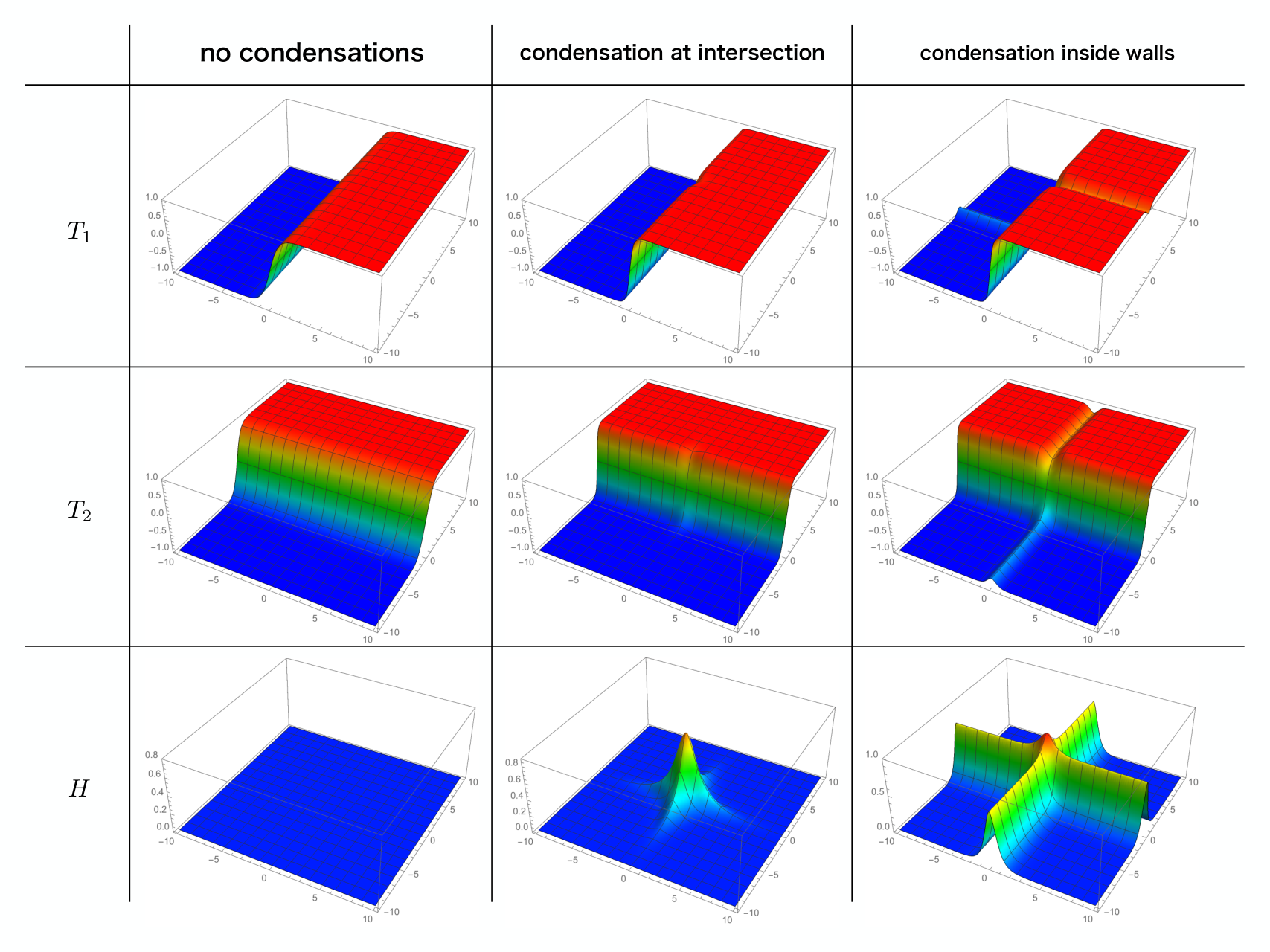
Depth of the potential is two folds: inside the each wall, and at the wall intersection. Thus, we expect that a tachyonic mode of appears, and it is localized either on the domain walls or only at the intersecting point according to . In order verify this observation, we numerically solved equations of motion for the model (254). The numerical solutions are shown in Fig. 6. We found three qualitatively different configurations. The first solution (the left column of Fig. 6) has no condensations at all. This appears when is sufficiently larger than . The second solution has finite condensation only around the intersecting point (the middle column of Fig. 6). The third solution has infinite condensation along the domain walls (the right column of Fig. 6). For our purpose of constructing four dimensional low energy theory, we prefer the finite condensation of whose codimension is two in six dimensions. Therefore, we will consider solutions of the type of middle column of Fig. 6.
Unfortunately, we do not have an analytic solution of the intersecting domain walls with a finite and non-zero condensation of . However, for an appropriate choice of parameters , and , we can make a simple separated approximation
| (257) |
with and being approximation parameters. We assume is the same order of . This product ansatz works very well as can be seen in Fig. 7 where we compare the numerical solution and the approximation with appropriate and .

With the above separable background condensation in Eq. (257) at hand, we will now investigate localization of the gauge field on the intersecting point through the Lagrangian
| (258) |
with
| (259) |
The separable property of the approximate function in and will help us to obtain the mass spectra below.
VI.1.1 Neutral stablizer
Here, we study the mass spectra of , , and for the model with the neutral stabilizer . All the formulae are given in Sec. III. As is given in Eq. (110), the mass spectrum for is determined by . Similarly, the mass spectrum of is determined by from Eq. (114). In general, and are different, but for the special choice of proportional to in Eq. (259) they are identical. To obtain their mass spectra, we will make use of the separable approximation for in Eq. (259). In this approximation, we have
| (260) |
Hence, the eigenvalue equation can be solved by separation of variables about and . The separated equations are identical to Eq. (42) which we have already analytically solved. There exists the unique zero eigenstate
| (261) |
All the excited states are continuum scattering modes as Eq. (44) whose masses are given by
| (262) |
The mass spectrum of the divergence-free part is determined by from Eq. (123), with
We have shown in Sec. III.2.3 that the mass spectrum of is identical to that of which can again be solved by separation of variables in and . For the specific given in Eq. (259), the problem becomes even simpler since has a constant potential:
| (267) |
Therefore, there are no bound states and the mass spectrum is given by
| (268) |
Thus, we conclude that the massless bound states localized at the intersection point are the four dimensional gauge field and the Nambu-Goldstone field . All other KK states from and are superheavy with the mass of order and are not localized.
VI.1.2 Charged stabilizer
We next study the same model as Eq. (254), but now the stabilizer is not neutral. So, we replace by . The mass spectrum of in this case is determined by , see Eq. (203). For the choice of in Eq. (259), is a constant
| (269) |
Thus, the masses of are all shifted by the constant from those of the neutral case. Namely, there is only one bound state which gets mass by the Higgs mechanism which locally occurs at the intersection point.
The remaining fields and are unified in , and the physical degrees of freedom are confined in . The mass spectrum of are identical to the eigenvalues of :
Following the general arguments of Sec. V, the eigenvalues of coincides with whose explicit form is given by
Hence, in contrast to and in the neutral case, there are no practical advantages to deal with instead of .
In order to obtain the mass spectra of the divergence free part, we make use of the generic argument given at the end of the Sec. V. According to them, the divergence free part can be decomposed into two orthogonal components as Eq. (V). The mass spectrum for the component associated with of (V) corresponds to the eigenvalues of , and the one for the other component corresponds to the eigenvalues of . In the six dimensions, we have and . Note that the non-zero eigenvalues of are identical to those of , if is separable. On the other hand, the non-zero eigenvalues of and are always identical. Therefore, for the separable , the two orthogonal components in the divergence free part (the first and the second term of Eq. (V)) are degenerate with eigenvalues of . Therefore, no light bound states exists and all the massive modes are heavy scattering modes whose masses are of order .
VI.2 Axially symmetric case
Our next example has that is not separable but is axially symmetric in the - plane. To be concrete, we assume the following Gaussian
| (282) |
Furthermore, we consider a specific as before
| (283) |
VI.2.1 Neutral stablizer
As before, we concentrate on , , and . All the formulae are given in Sec. III. For our special choice of proportional to in Eq. (283), and have the same mass eigenvalues of
| (284) |
with . The Schrödinger potential is asymptotically , so all the eigenstates are bound states. Eigenfunctions and eigenvalues of are given by
| (285) | |||||
| (286) | |||||
| (287) |
with is semi-positive integer and is an integer of . is the associated Laguerre polynomials. The zero mode is unique with with the wave function
| (288) |
VI.2.2 Charged stablizer
Next we consider the case that the stabilizer is charged. The masses of are identical to eigenvalues of the operator . For in Eq. (283), is constant. So, the effect of changing the neutral by the charged is just shift of all the eigenvalues of by the constant . This is the consequence of the local Higgs mechanism.
According to the generic arguments in Sec. V, the other physical degrees of freedom live in the divergence-free part . It can be further decomposed to two components orthogonal to each other: the component associated with and the other component associated with of (V). The former has the eigenvalues of , and the latter has the eigenvalues of . In the six dimensions, we have and its eigenvalues are given in Eq. (290). On the other hand, the non-zero eigenvalues of and are always identical, which is given in Eq. (287). Therefore, the mass spectra in are and with .
VII Conclusion
In this paper we investigated localization of the gauge fields via the field dependent gauge kinetic term (1) in details. We considered two cases that the stabilizers are neutral and charged. For the neutral case, we improved previous analysis done in Ref. Ohta:2010fu; Arai:2012cx; Arai:2013mwa; Arai:2014hda; Arai:2016jij; Arai:2017lfv; Arai:2017ntb, and especially analysis on the divergence-free parts becomes better, see Sec. II for , and Sec. III for generic . We also studied the models with charged stabilizers. The charged stabilizers are locally condensed inside a topological soliton, so that they localize the gauge fields and at the same time they give a finite mass to the localized gauge fields similarly to the conventional Higgs mechanism. In order to determine physical mass spectra, we need to diagonalize complicated mixings between the four-dimensional gauge fields, Nambu-Goldstone fields, and the extra-dimensional gauge fields which are further decomposed into the divergence and divergence-free parts. We developed complete and self-contained formula with which one can clearly separate physical and unphysical degrees of freedom for generic models in generic dimensions.
When we want massless gauge fields on a topological soliton, all we have to do is preparing neutral stabilizers which interact with the would-be localized gauge fields via Eq. (1). On the other hand, if we want to have massive gauge bosons on a topological soliton, it can be realized by just replacing the neutral stabilizers with the charged ones. An attempt of identifying the charged stabilizer with the SM Higgs boson in the model was studied in Ref. Arai:2018uoy.
Let us make a comment on localized gauge fields on domain walls in the Higgs vacua Tong:2002hi; Shifman:2002jm; Shifman:2003uh; Isozumi:2004jc; Isozumi:2004vg; Isozumi:2004va; Eto:2004vy; Tong:2005un; Eto:2006pg; Shifman:2007ce. When a domain wall interpolates two discrete Higgs vacua where the gauge symmetry is broken, the gauge symmetry is approximately recovered inside the domain wall. Nevertheless, the localized gauge field on the domain wall never becomes massless. The lowest mass of localized gauge field is inevitably of order inverse of the domain wall that is the same order of all the KK modes. Therefore, in principle, we cannot distinguish the lightest massive gauge bosons from the other KK modes. In contrast, the solitons in this work live in the confining vacua where the gauge symmetry is not broken. As we shown in this work, the lightest mass of localized gauge bosons is controlled only by the charge of the stabilizer, and it is nothing to do with the soliton width. Therefore, we can introduce two independent mass scales: the one is the lightest gauge boson mass and the other is superheavy mass of the KK towers. For phenomenological purpose, see for example Ref. Arai:2018uoy, our model has an advantage compared to other models with topological solitons in the Higgs phase.
As a future direction, it might be interesting to study the intersections of domain walls studied in Sec. VI. In this work, we only considered the intersection of two domain walls at right angle. In general, we can consider multiple domain walls, for example, three domain walls intersect at three different intersection points. We can also include fermions, and investigate whether such model provides a realist four dimensional model like intersecting D-branes Higaki:2005ie.
Acknowledgements
M. E. thanks to Masato Arai, Filip Blaschke, and Norisuke Sakai for fruitful discussions throughout long collaboration, and contributions at the early stage of this work. The work is supported in part by JSPS Grant-in-Aid for Scientific Research KAKENHI Grant No. JP16H03984 and No. JP19K03839. The work is also supported in part by MEXT KAKENHI Grant-in-Aid for Scientific Research on Innovative Areas Discrete Geometric Analysis for Materials Design No. JP17H06462 from the MEXT of Japan.
References
- (1) N. Arkani-Hamed, S. Dimopoulos and G. R. Dvali, “The Hierarchy problem and new dimensions at a millimeter,” Phys. Lett. B 429, 263 (1998) doi:10.1016/S0370-2693(98)00466-3 [hep-ph/9803315].
- (2) I. Antoniadis, N. Arkani-Hamed, S. Dimopoulos and G. R. Dvali, “New dimensions at a millimeter to a Fermi and superstrings at a TeV,” Phys. Lett. B 436, 257 (1998) doi:10.1016/S0370-2693(98)00860-0 [hep-ph/9804398].
- (3) L. Randall and R. Sundrum, “A Large mass hierarchy from a small extra dimension,” Phys. Rev. Lett. 83, 3370 (1999) doi:10.1103/PhysRevLett.83.3370 [hep-ph/9905221].
- (4) L. Randall and R. Sundrum, “An Alternative to compactification,” Phys. Rev. Lett. 83, 4690 (1999) doi:10.1103/PhysRevLett.83.4690 [hep-th/9906064].
- (5) V. A. Rubakov and M. E. Shaposhnikov, “Do We Live Inside a Domain Wall?,” Phys. Lett. 125B, 136 (1983). doi:10.1016/0370-2693(83)91253-4.
- (6) R. Jackiw and C. Rebbi, “Solitons with Fermion Number 1/2,” Phys. Rev. D 13, 3398 (1976). doi:10.1103/PhysRevD.13.3398.
- (7) M. Cvetic, S. Griffies and S. J. Rey, “Static domain walls in N=1 supergravity,” Nucl. Phys. B 381, 301 (1992) doi:10.1016/0550-3213(92)90649-V [hep-th/9201007].
- (8) O. DeWolfe, D. Z. Freedman, S. S. Gubser and A. Karch, “Modeling the fifth-dimension with scalars and gravity,” Phys. Rev. D 62, 046008 (2000) doi:10.1103/PhysRevD.62.046008 [hep-th/9909134].
- (9) C. Csaki, J. Erlich, T. J. Hollowood and Y. Shirman, “Universal aspects of gravity localized on thick branes,” Nucl. Phys. B 581, 309 (2000) doi:10.1016/S0550-3213(00)00271-6 [hep-th/0001033].
- (10) M. Eto, N. Maru, N. Sakai and T. Sakata, “Exactly solved BPS wall and winding number in N=1 supergravity,” Phys. Lett. B 553, 87 (2003) doi:10.1016/S0370-2693(02)03187-8 [hep-th/0208127].
- (11) M. Eto, S. Fujita, M. Naganuma and N. Sakai, “BPS Multi-walls in five-dimensional supergravity,” Phys. Rev. D 69, 025007 (2004) doi:10.1103/PhysRevD.69.025007 [hep-th/0306198].
- (12) M. Eto and N. Sakai, “Solvable models of domain walls in N = 1 supergravity,” Phys. Rev. D 68, 125001 (2003) doi:10.1103/PhysRevD.68.125001 [hep-th/0307276].
- (13) G. R. Dvali, G. Gabadadze and M. A. Shifman, “(Quasi)localized gauge field on a brane: Dissipating cosmic radiation to extra dimensions?,” Phys. Lett. B 497, 271 (2001) doi:10.1016/S0370-2693(00)01329-0 [hep-th/0010071].
- (14) A. Kehagias and K. Tamvakis, “Localized gravitons, gauge bosons and chiral fermions in smooth spaces generated by a bounce,” Phys. Lett. B 504, 38 (2001) doi:10.1016/S0370-2693(01)00274-X [hep-th/0010112].
- (15) S. L. Dubovsky and V. A. Rubakov, “On models of gauge field localization on a brane,” Int. J. Mod. Phys. A 16, 4331 (2001) doi:10.1142/S0217751X01005286 [hep-th/0105243].
- (16) K. Ghoroku and A. Nakamura, “Massive vector trapping as a gauge boson on a brane,” Phys. Rev. D 65, 084017 (2002) doi:10.1103/PhysRevD.65.084017 [hep-th/0106145].
- (17) E. K. Akhmedov, “Dynamical localization of gauge fields on a brane,” Phys. Lett. B 521, 79 (2001) doi:10.1016/S0370-2693(01)01176-5 [hep-th/0107223].
- (18) I. I. Kogan, S. Mouslopoulos, A. Papazoglou and G. G. Ross, “Multilocalization in multibrane worlds,” Nucl. Phys. B 615, 191 (2001) doi:10.1016/S0550-3213(01)00424-2 [hep-ph/0107307].
- (19) H. Abe, T. Kobayashi, N. Maru and K. Yoshioka, “Field localization in warped gauge theories,” Phys. Rev. D 67, 045019 (2003) doi:10.1103/PhysRevD.67.045019 [hep-ph/0205344].
- (20) M. Laine, H. B. Meyer, K. Rummukainen and M. Shaposhnikov, “Localization and mass generation for nonAbelian gauge fields,” JHEP 0301, 068 (2003) doi:10.1088/1126-6708/2003/01/068 [hep-ph/0211149].
- (21) N. Maru and N. Sakai, “Localized gauge multiplet on a wall,” Prog. Theor. Phys. 111, 907 (2004) doi:10.1143/PTP.111.907 [hep-th/0305222].
- (22) B. Batell and T. Gherghetta, “Yang-Mills Localization in Warped Space,” Phys. Rev. D 75, 025022 (2007) doi:10.1103/PhysRevD.75.025022 [hep-th/0611305].
- (23) R. Guerrero, A. Melfo, N. Pantoja and R. O. Rodriguez, “Gauge field localization on brane worlds,” Phys. Rev. D 81, 086004 (2010) doi:10.1103/PhysRevD.81.086004 [arXiv:0912.0463 [hep-th]].
- (24) W. T. Cruz, M. O. Tahim and C. A. S. Almeida, “Gauge field localization on a dilatonic deformed brane,” Phys. Lett. B 686, 259 (2010). doi:10.1016/j.physletb.2010.02.064
- (25) A. E. R. Chumbes, J. M. Hoff da Silva and M. B. Hott, “A model to localize gauge and tensor fields on thick branes,” Phys. Rev. D 85, 085003 (2012) doi:10.1103/PhysRevD.85.085003 [arXiv:1108.3821 [hep-th]].
- (26) C. Germani, “Spontaneous localization on a brane via a gravitational mechanism,” Phys. Rev. D 85, 055025 (2012) doi:10.1103/PhysRevD.85.055025 [arXiv:1109.3718 [hep-ph]].
- (27) T. Delsate and N. Sawado, “Localizing modes of massive fermions and a U(1) gauge field in the inflating baby-skyrmion branes,” Phys. Rev. D 85, 065025 (2012) doi:10.1103/PhysRevD.85.065025 [arXiv:1112.2714 [gr-qc]].
- (28) W. T. Cruz, A. R. P. Lima and C. A. S. Almeida, Phys. Rev. D 87, no. 4, 045018 (2013) doi:10.1103/PhysRevD.87.045018 [arXiv:1211.7355 [hep-th]].
- (29) A. Herrera-Aguilar, A. D. Rojas and E. Santos-Rodriguez, “Localization of gauge fields in a tachyonic de Sitter thick braneworld,” Eur. Phys. J. C 74, no. 4, 2770 (2014) doi:10.1140/epjc/s10052-014-2770-1 [arXiv:1401.0999 [hep-th]].
- (30) Z. H. Zhao, Y. X. Liu and Y. Zhong, “U(1) gauge field localization on a Bloch brane with Chumbes-Holf da Silva-Hott mechanism,” Phys. Rev. D 90, no. 4, 045031 (2014) doi:10.1103/PhysRevD.90.045031 [arXiv:1402.6480 [hep-th]].
- (31) C. A. Vaquera-Araujo and O. Corradini, “Localization of abelian gauge fields on thick branes,” Eur. Phys. J. C 75, no. 2, 48 (2015) doi:10.1140/epjc/s10052-014-3251-2 [arXiv:1406.2892 [hep-th]].
- (32) G. Alencar, R. R. Landim, M. O. Tahim and R. N. Costa Filho, “Gauge Field Localization on the Brane Through Geometrical Coupling,” Phys. Lett. B 739, 125 (2014) doi:10.1016/j.physletb.2014.10.040 [arXiv:1409.4396 [hep-th]].
- (33) G. Alencar, R. R. Landim, C. R. Muniz and R. N. Costa Filho, “Nonminimal couplings in Randall-Sundrum scenarios,” Phys. Rev. D 92, no. 6, 066006 (2015) doi:10.1103/PhysRevD.92.066006 [arXiv:1502.02998 [hep-th]].
- (34) G. Alencar, I. C. Jardim, R. R. Landim, C. R. Muniz and R. N. Costa Filho, “Generalized nonminimal couplings in Randall-Sundrum scenarios,” Phys. Rev. D 93, no. 12, 124064 (2016) doi:10.1103/PhysRevD.93.124064 [arXiv:1506.00622 [hep-th]].
- (35) G. Alencar, C. R. Muniz, R. R. Landim, I. C. Jardim and R. N. Costa Filho, “Photon mass as a probe to extra dimensions,” Phys. Lett. B 759, 138 (2016) doi:10.1016/j.physletb.2016.05.062 [arXiv:1511.03608 [hep-th]].
- (36) G. Alencar, “Hidden conformal symmetry in Randall-Sundrum 2 model: Universal fermion localization by torsion,” Phys. Lett. B 773, 601 (2017) doi:10.1016/j.physletb.2017.09.014 [arXiv:1705.09331 [hep-th]].
- (37) K. Ohta and N. Sakai, “Non-Abelian Gauge Field Localized on Walls with Four-Dimensional World Volume,” Prog. Theor. Phys. 124, 71 (2010) Erratum: [Prog. Theor. Phys. 127, 1133 (2012)] doi:10.1143/PTP.124.71 [arXiv:1004.4078 [hep-th]].
- (38) M. A. Luty and N. Okada, “Almost no scale supergravity,” JHEP 0304, 050 (2003) doi:10.1088/1126-6708/2003/04/050 [hep-th/0209178].
- (39) G. R. Dvali and M. A. Shifman, “Domain walls in strongly coupled theories,” Phys. Lett. B 396, 64 (1997) Erratum: [Phys. Lett. B 407, 452 (1997)] doi:10.1016/S0370-2693(97)00808-3, 10.1016/S0370-2693(97)00131-7 [hep-th/9612128].
- (40) J. B. Kogut and L. Susskind, “Vacuum Polarization and the Absence of Free Quarks in Four-Dimensions,” Phys. Rev. D 9, 3501 (1974). doi:10.1103/PhysRevD.9.3501
- (41) R. Fukuda, “String-Like Phase in Yang-Mills Theory,” Phys. Lett. 73B, 305 (1978) Erratum: [Phys. Lett. 74B, 433 (1978)]. doi:10.1016/0370-2693(78)90521-X
- (42) R. Fukuda, “Stability of the vacuum and dielectric model of confinement in QCD,” Mod. Phys. Lett. A 24, 251 (2009). doi:10.1142/S0217732309030035
- (43) R. Fukuda, “Derivation of Dielectric Model of Confinement in QCD,” arXiv:0805.3864 [hep-th].
- (44) M. Arai, F. Blaschke, M. Eto and N. Sakai, “Matter Fields and Non-Abelian Gauge Fields Localized on Walls,” PTEP 2013, 013B05 (2013) doi:10.1093/ptep/pts050 [arXiv:1208.6219 [hep-th]].
- (45) M. Arai, F. Blaschke, M. Eto and N. Sakai, “Stabilizing matter and gauge fields localized on walls,” PTEP 2013, no. 9, 093B01 (2013) doi:10.1093/ptep/ptt064 [arXiv:1303.5212 [hep-th]].
- (46) M. Arai, F. Blaschke, M. Eto and N. Sakai, “Dynamics of slender monopoles and anti-monopoles in non-Abelian superconductor,” JHEP 1409, 172 (2014) doi:10.1007/JHEP09(2014)172 [arXiv:1407.2332 [hep-th]].
- (47) M. Arai, F. Blaschke, M. Eto and N. Sakai, J. Phys. Conf. Ser. 670, no. 1, 012006 (2016). doi:10.1088/1742-6596/670/1/012006
- (48) M. Arai, F. Blaschke, M. Eto and N. Sakai, “Non-Abelian Gauge Field Localization on Walls and Geometric Higgs Mechanism,” PTEP 2017, no. 5, 053B01 (2017) doi:10.1093/ptep/ptx047 [arXiv:1703.00427 [hep-th]].
- (49) M. Arai, F. Blaschke, M. Eto and N. Sakai, “Grand Unified Brane World Scenario,” Phys. Rev. D 96, no. 11, 115033 (2017) doi:10.1103/PhysRevD.96.115033 [arXiv:1703.00351 [hep-th]].
- (50) M. Arai, F. Blaschke, M. Eto and N. Sakai, “Localized non-Abelian gauge fields in non-compact extra-dimensions,” arXiv:1801.02498 [hep-th].
- (51) M. Arai, F. Blaschke, M. Eto and N. Sakai, “Localization of the Standard Model via the Higgs mechanism and a finite electroweak monopole from non-compact five dimensions,” PTEP 2018, no. 8, 083B04 (2018) doi:10.1093/ptep/pty083 [arXiv:1802.06649 [hep-ph]].
- (52) M. Arai, F. Blaschke, M. Eto and N. Sakai, “Topological massless bosons on edges: Jackiw-Rebbi mechanism for bosonic fields,” arXiv:1811.08708 [hep-th].
- (53) N. Okada, D. Raut and D. Villalba, “Domain-Wall Standard Model and LHC,” arXiv:1712.09323 [hep-ph].
- (54) N. Okada, D. Raut and D. Villalba, “Aspects of Domain-Wall Standard Model,” arXiv:1801.03007 [hep-ph].
- (55) N. Okada, D. Raut and D. Villalba, “Fermion Mass Hierarchy and Phenomenology in the 5D Domain Wall Standard Model,” arXiv:1904.10308 [hep-ph].
- (56) J. P. Gauntlett, D. Tong and P. K. Townsend, “Supersymmetric intersecting domain walls in massive hyperKahler sigma models,” Phys. Rev. D 63, 085001 (2001) doi:10.1103/PhysRevD.63.085001 [hep-th/0007124].
- (57) J. P. Gauntlett, D. Tong and P. K. Townsend, “Multidomain walls in massive supersymmetric sigma models,” Phys. Rev. D 64, 025010 (2001) doi:10.1103/PhysRevD.64.025010 [hep-th/0012178].
- (58) M. Eto, Y. Isozumi, M. Nitta and K. Ohashi, “1/2, 1/4 and 1/8 BPS equations in SUSY Yang-Mills-Higgs systems: Field theoretical brane configurations,” Nucl. Phys. B 752, 140 (2006) doi:10.1016/j.nuclphysb.2006.06.026 [hep-th/0506257].
- (59) M. Eto, Y. Isozumi, M. Nitta, K. Ohashi and N. Sakai, “Solitons in the Higgs phase: The Moduli matrix approach,” J. Phys. A 39, R315 (2006) doi:10.1088/0305-4470/39/26/R01 [hep-th/0602170].
- (60) D. Tong, Phys. Rev. D 66, 025013 (2002) doi:10.1103/PhysRevD.66.025013 [hep-th/0202012].
- (61) M. Shifman and A. Yung, “Domain walls and flux tubes in N=2 SQCD: D-brane prototypes,” Phys. Rev. D 67, 125007 (2003) doi:10.1103/PhysRevD.67.125007 [hep-th/0212293].
- (62) M. Shifman and A. Yung, “Localization of nonAbelian gauge fields on domain walls at weak coupling (D-brane prototypes II),” Phys. Rev. D 70, 025013 (2004) doi:10.1103/PhysRevD.70.025013 [hep-th/0312257].
- (63) Y. Isozumi, M. Nitta, K. Ohashi and N. Sakai, “Construction of non-Abelian walls and their complete moduli space,” Phys. Rev. Lett. 93, 161601 (2004) doi:10.1103/PhysRevLett.93.161601 [hep-th/0404198].
- (64) Y. Isozumi, M. Nitta, K. Ohashi and N. Sakai, Phys. Rev. D 71, 065018 (2005) doi:10.1103/PhysRevD.71.065018 [hep-th/0405129].
- (65) Y. Isozumi, M. Nitta, K. Ohashi and N. Sakai, “Non-Abelian walls in supersymmetric gauge theories,” Phys. Rev. D 70, 125014 (2004) doi:10.1103/PhysRevD.70.125014 [hep-th/0405194].
- (66) M. Eto, Y. Isozumi, M. Nitta, K. Ohashi, K. Ohta and N. Sakai, “D-brane construction for non-Abelian walls,” Phys. Rev. D 71, 125006 (2005) doi:10.1103/PhysRevD.71.125006 [hep-th/0412024].
- (67) D. Tong, “TASI lectures on solitons: Instantons, monopoles, vortices and kinks,” hep-th/0509216.
- (68) M. Shifman and A. Yung, “Supersymmetric Solitons and How They Help Us Understand Non-Abelian Gauge Theories,” Rev. Mod. Phys. 79, 1139 (2007) doi:10.1103/RevModPhys.79.1139 [hep-th/0703267].
- (69) T. Higaki, N. Kitazawa, T. Kobayashi and K. j. Takahashi, “Flavor structure and coupling selection rule from intersecting D-branes,” Phys. Rev. D 72, 086003 (2005) doi:10.1103/PhysRevD.72.086003 [hep-th/0504019].