Universal Interferometric Signatures of a Black Hole’s Photon Ring
Abstract
The Event Horizon Telescope image of the supermassive black hole in the galaxy M87 is dominated by a bright, unresolved ring. General relativity predicts that embedded within this image lies a thin “photon ring,” which is composed of an infinite sequence of self-similar subrings that are indexed by the number of photon orbits around the black hole. The subrings approach the edge of the black hole “shadow,” becoming exponentially narrower but weaker with increasing orbit number, with seemingly negligible contributions from high order subrings. Here, we show that these subrings produce strong and universal signatures on long interferometric baselines. These signatures offer the possibility of precise measurements of black hole mass and spin, as well as tests of general relativity, using only a sparse interferometric array.
Subject headings
black hole physics — radio continuum: Galaxy: nucleus — techniques: interferometricI. Introduction
The EHT Collaboration has recently published images of the supermassive black hole in M87 using Very Long Baseline Interferometry (VLBI) at 1.3 mm wavelength (Event Horizon Telescope Collaboration et al. 2019a; Event Horizon Telescope Collaboration et al. 2019b; Event Horizon Telescope Collaboration et al. 2019c; Event Horizon Telescope Collaboration et al. 2019d; Event Horizon Telescope Collaboration et al. 2019e; Event Horizon Telescope Collaboration et al. 2019f; hereafter Paper I-VI). These images reveal a bright ring of emission with a diameter of approximately . However, while the diameter of this ring is resolved by the EHT, its thickness and detailed substructure are not. In this Letter, we show that general relativity predicts an intricate substructure within this ring that presents distinctive signatures for interferometric measurements. These signatures offer a promising approach for precisely determining the masses and spins of black holes and for testing general relativity using sparse interferometers, such as an extension of the EHT to space.
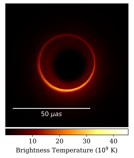
Neglecting opacity, a telescope with perfect resolution directed at a black hole observes an infinite number of nested images of the universe. These images arise from photons that differ by the number of half-orbits they complete around the black hole on the way from their source to the detector. Each such image is thus an increasingly delayed and demagnified snapshot of the universe as seen from the black hole. In an astrophysical setting, this self-similar sequence of relativistic images is dominated by the luminous matter surrounding the black hole and produces in its image a feature known as the “photon ring” of the black hole (Bardeen 1973; Luminet 1979; Johannsen & Psaltis 2010; Gralla et al. 2019). The leading () subring appears as a sharp, bright feature in ray-traced images from many general-relativistic magnetohydrodynamic (GRMHD) simulations (see Figure 1). Successive subrings have exponentially sharper profiles and asymptotically approach the boundary of the black hole “shadow”. For large , these profiles mirror the leading subring in a manner that depends universally on the spacetime geometry, with the ratio of successive subring flux densities determined by Lyapunov exponents that characterize the instability of bound photon orbits. Hence, measuring the size, shape, and thickness of the subrings would provide new and powerful probes of a black hole spacetime.
Both GRMHD simulations and analytic estimates suggest that the photon ring should provide only 10% of the total image flux density. This dimness may appear to preclude observations of the photon ring and its substructure, which is dimmer still. However, interferometric measurements are sensitive to more than just overall flux: they also natively filter images by their spatial wavenumbers, and therefore naturally isolate contributions from individual photon subrings. Sufficiently long baselines also resolve out diffuse flux in an image, and are thus dominated by power from the photon ring. Hence, even though sharp elements of the photon ring produce a negligible contribution to the total flux in an image, they can still provide a pronounced, dominant signal on long baselines.
In this Letter, we explore the photon ring’s theoretical underpinnings and show that, surprisingly, precise measurements of the photon ring and even its subrings are feasible using interferometry. In §II, we describe the shell of bound photon orbits of a Kerr black hole and its relation to the photon ring. We also present a decomposition of the photon ring into subrings indexed by half-orbit number and derive their self-similar structure, which is universally governed by Lyapunov exponents that characterize orbital instability. Next, in §III, we derive generically expected interferometric signatures of the photon ring. We show that its subrings produce a cascade of damped oscillations on progressively longer baselines, with the visibility of each subring conveying precise information about its diameter, width, and angular profile. Finally, in §IV, we discuss observational prospects for detecting these signatures with extensions of the EHT. In particular, we highlight the possibility of detecting the leading subring using a station in low Earth orbit, the subring using a station on the Moon, and the subring using a station in the Sun-Earth orbit.
II. Photon Shell and Photon Ring

This section describes the shell of unstable bound photon orbits surrounding a black hole, its lensed photon ring image, the photon subrings labeled by half-orbit number, and the angle-dependent Lyapunov exponents that govern the subring brightness ratio asymmetry. Previous treatments of these structures include Darwin 1959; Bardeen et al. 1972; Luminet 1979; Teo 2003; Gralla et al. 2019. Observational aspects of these features follow in §III and §IV.
II.1. Photon Shell
The photon shell, illustrated in Figure 2, is the region of a black hole spacetime containing bound null geodesics or “bound orbits” that neither escape to infinity nor fall across the event horizon. For Schwarzschild, the photon shell is the two-dimensional sphere at and any , and . For Kerr, this two-dimensional sphere fattens to a three-dimensional spherical shell. It is best described using Boyer-Lindquist coordinates, in which the metric of a Kerr black hole of mass and angular momentum (with ) is
| (1a) | |||
| (1b) | |||
These coordinates have the special property that all bound orbits lie at some fixed value of in the range
| (2a) | ||||
| (2b) | ||||
Every point in the equatorial annulus , has a unique bound orbit passing through it. On the boundaries , the orbits reside entirely in the equatorial plane. At generic points, on the other hand, they oscillate in the -direction between polar angles
| (3) |
where
| (4) | ||||
We will refer to one such complete oscillation (, from back to itself) as one orbit, since the photon typically returns to a point near, but not identical to (since the azimuthal angle also shifts), its initial position.
The bound orbit at radius has the energy-rescaled angular momentum
| (6) |
The inner circular equatorial orbit at is prograde, while the outer one at is retrograde: . The overall direction of the orbits reverses at the intermediate value for which vanishes. At that radius, equals and the orbits can pass over the poles.
The bound geodesics are unstable in the sense that, if perturbed slightly, they either fall into the black hole or escape to infinity where they can reach a telescope. The observed photon ring image arises from photons traveling on such “nearly bound” geodesics. Consider two geodesics, one of which is bound, with the other initially differing only by an infinitesimal radial separation . The equation of geodesic deviation shows that, after half-orbits between , their separation grows to
| (7) |
Here, the so-called Lyapunov exponent is a function on the space of bound orbits given by11 1 A closely related formula appears in Yang et al. 2012. (see Appendix A.1)
| (8) |
Hence, the nearly-bound geodesic will typically cross the equatorial plane a number of times of order
| (9) |
until , when the geodesic is well-separated from the bound orbit and it shoots off to infinity (or crosses the event horizon if ). These Lyapunov exponents are central and potentially observable quantities that characterize the geometry of the Kerr photon shell.
II.2. Photon Ring and Subrings
The photon ring is the image on the observer screen (Bardeen 1973; as described by) produced by photons on nearly bound geodesics. In the limit in which the photons become fully bound, it may be shown that their images approach a closed curve given by
| (10a) | ||||
| (10b) | ||||
where are dimensionless polar coordinates on the observer screen, while denote the observer’s distance and inclination from the Kerr spin axis. We can view as parameterized by the shell radius from which the photon originated. For each value of , (10) has two solutions for in the range , so each radius in the photon shell appears at two positions on . A striking consequence of (10) is that for , both and , and hence , are functions only of , , and . Hence, a measurement at a specific angle along the ring probes a specific radius of the Kerr geometry and not, as might have been expected, a specific angle around the black hole!
Astrophysically observed photon intensities at the screen can be computed by backward ray-tracing. One follows the null geodesics from the observer screen back into the Kerr spacetime, integrating the Doppler-shifted strength of matter sources along the geodesic, with attenuation factors accounting for the optical depth (Mościbrodzka & Gammie 2018; for the images in this paper, we used ipole;).22 2 Scattering effects are negligible because the expected plasma frequency and electron gyroradius are in the MHz range, several orders of magnitude below the observing frequencies we consider. A light ray aimed exactly at the curve is captured by the photon shell and (unstably) orbits the black hole forever. Those aimed inside fall into the black hole, while those aimed outside escape to infinity. Therefore, is the edge of the black hole “shadow”.
If we shoot a light ray very near, a distance from the shadow edge at , it will circle many times through the emission region before falling into the black hole or escaping to infinity. The affine length of the ray and its number of half-orbits accordingly diverge as :
| (11) |
This follows from (9) together with a computed relation between and . For optically thin matter distributions, (11) implies a mild divergence in the observed ring intensity as the shadow edge is approached, since a light ray that completes half-orbits through the emission region can collect times more photons along its path. The photon ring is then the bump in the photon intensity containing this logarithmic divergence at the shadow edge. Although the divergence is cut off by a finite optical depth, this striking feature remains visually prominent in many ray-traced images of GRMHD simulations, as in Figure 1.
The photon ring can be subdivided into subrings arising from photons that have completed half-orbits between their source and the screen.33 3 This definition for the photon ring agrees with that in Beckwith & Done 2005, but differs from the later usage in Johannsen & Psaltis 2010 and Gralla et al. 2019 by the inclusion of the and 2 contributions. These low contributions fully account for the thin ring image visible in Figure 1. In order to orbit at least times around the black hole, the photon must be aimed within an exponentially narrowing window
| (12) |
around the shadow edge. Hence, the subrings occupy a sequence of exponentially nested intervals centered around .
Each subring consists of photons lensed towards the observer screen after having been collected by the photon shell from anywhere in the universe. Hence, in an idealized setting with no absorption, each subring contains a separate, exponentially demagnified image of the entire universe, with each subsequent subring capturing the visible universe at an earlier time. Together, the set of subrings are akin to the frames of a movie, capturing the history of the visible universe as seen from the black hole. In an astrophysical setting, these images are dominated by the luminous matter around the black hole. For a black hole surrounded by a uniform distribution extending over the poles, the contributions made by each subring to the total intensity profile cannot be told apart, and the individual subrings cannot be distinguished on the image. However, for a realistic disk or jet with emission peaked in a conical region, the subrings are visibly distinct: the subring is approximately a smooth peak of width . Summing these smooth peaks, like layers in a tiered wedding cake (see Figure 3), reproduces the leading logarithmic divergence (11) in the intensity.
The photons comprising successive subrings for the same angle traverse essentially the same orbits, and hence encounter the same matter distribution around the black hole. Apart from source variations on the timescale of an orbit, intensities of the and subring differ only because they correspond to windows whose widths and differ by a factor of . Hence, for large enough , the intensities are related by
| (13) |
Integrating a radial slice across the subring, we therefore find the angle-dependent subring flux ratio
| (14) |
(13) and (14) are matter-independent predictions for the photon ring structure that involve only general relativity. The prediction holds only for “large enough” : at small , there are non-universal matter-dependent effects from photons that do not traverse exactly the same region around the black hole. Insight into when is “large enough” might be obtained from GRMHD simulations.
Since the exponent depends on , and , the flux ratio asymmetry in (14) provides a new method for determination of the spin. For Schwarzschild, (Luminet 1979), corresponding to a demagnification factor of . For a black hole of maximal spin viewed from an inclination (Walker et al. 2018; as estimated for M87;), the factor is as large as 13% on the part of the ring where the black hole spins towards the observer. Although (12) breaks down for , this suppression factor suggests that the leading subring should provide of the total luminosity, in order-of-magnitude agreement with GRMHD simulations.

III. Interferometric Signatures of a Photon Ring
This section explores the response of an interferometer to the photon ring described in §II through a series of increasingly refined geometrical models. We first review the interferometric signatures of an infinitesimally thin, uniform, circular ring (§III.1). We then extend this treatment to include rings with non-uniform brightness (§III.2), non-zero thickness (§III.3), and non-circular structure (§III.4). We conclude this section by discussing specific features expected for the photon ring and its subrings (§III.5). The prospects for experimental detection of these features are addressed in §IV.
III.1. Visibilities for a Thin, Uniform, Circular Ring
Each baseline joining two elements of an interferometer samples a complex visibility , which corresponds to a single Fourier component of the sky image (Thompson et al. 2017):
| (15) |
Here, is the dimensionless vector baseline projected orthogonal to the line of sight and measured in units of the observation wavelength , while is a dimensionless image coordinate measured in radians.
In terms of polar coordinates on the observer screen (10), the image and corresponding visibility function of an infinitesimally thin, uniform, circular ring are
| (16a) | ||||
| (16b) | ||||
where is the ring diameter in radians and the image is normalized to have a total flux density of unity, . denotes the Bessel function of the first kind, which admits the asymptotic expansion
| (17) |
valid for . Hence, is a weakly damped pure frequency with period inside an envelope that falls as .
III.2. Visibilities for a Non-Uniform Ring
The image of a thin ring with non-uniform brightness in decomposes into a sum over angular Fourier modes,
| (18) |
where since the image is real. The total image flux density is given by .
The corresponding visibility function is
| (19) |
Using (17), for long baselines we may approximate
| (20) |
Thus, for sufficiently long baselines, the radial visibility function of a non-uniform thin ring is determined by a single pair of weakly damped, orthogonal modes . Their envelope still falls as , and the modes have a common period of in complex visibilities (or in visibility amplitudes). The angular spectrum of the image is easily retrieved from the angular spectrum of the visibilities (see Appendix B.2).


III.3. Visibilities for a Thick Ring
Baselines of length are required in order to resolve image features of size . Hence, the visibility function of any ring with diameter and thickness has two asymptotic regimes:
| (21) |
Baselines in regime (I) resolve the diameter of the ring but not its thickness, while longer baselines in regime (II) resolve both. As such, the visibility function in regime (I) behaves like that of a thin ring (a damped periodicity with envelope ), while the envelope of the visibility function in regime (II) is sensitive to the radial profile of the ring. In general, the visibility of any smooth ring decays exponentially in regime (II).44 4 Images with discontinuous derivatives, such as a uniform disk or annulus, can have slower, power-law falloffs.
The validity of the approximation (17) in regime (I) depends on the amount of power at high values of . Specifically, it requires . Under this condition, has periods in regime (I).
III.4. Visibilities for a Non-Circular Ring
Although the photon ring is nearly circular for all black hole spins and inclinations, the primary interferometric signatures discussed thus far do not require an image with perfectly circular structure. For instance, if an image is stretched, , then its visibility function is correspondingly compressed, . Thus, the visibility profiles of a stretched ring share the properties and asymptotic expansions derived for a circular ring [, (III.2)], except that the radial periodicities become a function of position angle. To leading order in the asymmetry , the diameter corresponding to a damped radial periodicity in the visibility domain matches that of the stretched ring along the baseline’s position angle. For the black hole in M87, the asymmetry is expected to be a few percent at most, even for a maximally rotating black hole (see Figure 7).
III.5. Visibilities of the Photon Subrings
As discussed in §II.2, the photon ring decomposes into subrings labelled by the photon half-orbit number . This section describes the distinctive and universal interferometric signatures of these subrings.
According to (14), the width of the radial intensity profile produced by the subring is while the brightness remains approximately constant with (until some determined by the optical depth). Each subring thus contributes a periodically modulated visibility, , which falls more steeply for baselines (see §III.3). Hence, the subring dominates the signal in the regime
| (22) |
This implies that the totality of subring contributions has an envelope defined by this turnover behavior:
| (23) |
Together, the subrings then form a cascade of damped oscillations on progressively longer baselines, each dominated by the image of a single subring and conveying precise information about its diameter, thickness, and angular profile. Figure 4 displays visibilities of the time-averaged GRMHD image in Figure 1, which exhibit the expected damped periodicity, as well as clear contributions on long baselines from distinct subrings. See Figure 5 for a schematic illustration of this cascade.
IV. Observational Prospects and Considerations

Detection of the photon ring’s universal interferometric signatures requires measurements on longer baselines, with finer angular resolution than those currently available to the EHT. This extension can be achieved either by observing at higher frequencies55 5 ALMA currently observes up to 950 GHz (ALMA band 10) with higher frequencies (up to 1.53 THz) possible in the future (Wiedner et al. 2007; Rigopoulou et al. 2013; see, ,). or by observing on longer physical baselines via space-VLBI. Figure 5 shows baseline lengths for a variety of array configurations and observing frequencies.
For the EHT to observe the photon ring, it must also achieve sufficient sensitivity to detect its visibilities. For both Sgr A∗ and M87, the horizon-scale emission has a total flux density of at (Bower et al. 2015; Chael et al. 2019; see, e.g.,), with a fraction expected to come from the photon ring (see §II and 14). The expected amplitude of the photon ring on long interferometric baselines is thus
| (24) | ||||
For comparison, a baseline from ALMA to a 4-meter orbiter with 32 GHz of averaged bandwidth and a 10-minute coherent integration would have thermal noise of at 950 GHz and at 690 GHz. For baselines from ALMA to a 10-meter orbiter, such as the proposed Millimetron mission for (Wild et al. 2009; Kardashev et al. 2014), the thermal noise would be and . Another possibility would be to place a VLBI station on or orbiting the Moon, which could sample many periods of the regime of M87 at current EHT observing frequencies. A 10-meter dish on the Moon could achieve on baselines to ALMA with coherent integrations of 10 minutes and a bandwidth of 32 GHz. These sensitivities could be significantly improved via simultaneous multi-frequency observations. In addition to having more sensitive receivers and longer coherence times, lower frequencies give correspondingly shorter baselines and, thus, increased interferometric power from the photon ring. Phase calibration with lower frequencies could then allow substantially longer integration times at higher frequencies. See Appendix C for additional details and discussion.
Interferometric signatures of the photon ring are most prominent when the image has little small-scale power outside the ring, and when the ring has a smooth angular profile dominated by low mode-numbers . Both of these conditions are met in time-averaged images of black hole accretion flows, such as Figure 1. Because visibilities of a time-averaged image are equal to time-averaged visibilities of a variable image, developing capabilities for long, coherent averaging could significantly improve the prospects for unambiguous detection and characterization of the photon ring.
In summary, precise measurements of the size, shape, thickness, and angular profile of the photon subring of M87 and Sgr A∗ may be feasible for using a high-frequency ground array or low Earth orbits, for with a station on the Moon, and for with a station in .
Appendix A Properties of the Photon Shell
A.1. Geodesic Deviation From Bound Orbits
This section derives the Lyapunov exponent (8) that governs the exponential geodesic deviation (7), using the same conventions as Kapec & Lupsasca 2019. Figure 6 shows the Lyapunov exponent for selected values of black hole spin and inclination.
A Kerr geodesic connecting to satisfies
| (A1) |
where and are potentials for the radial and polar motions, respectively, and the slash notation indicates that these integrals are to be evaluated along the geodesic, with turning points in each motion occurring whenever the corresponding potential vanishes.
Bound orbits occur at double roots of the radial potential where . For the bound orbit at radius , the angular integral, evaluated over one half-orbit, is the complete elliptic integral of the first kind
| (A2) |
Consider a nearby photon on a nearly bound geodesic, initially at a radius infinitesimally close to the bound orbit (). After half-orbits, it advances to the larger radius such that
| (A3) |
Since for the nearly bound geodesic, the radial integral is approximately
| (A4) |
It follows that the photon’s radial deviation from the bound orbit at radius grows exponentially, with Lyapunov exponent
| (A5) |
A.2. Edge of the Black Hole Shadow
Inverting the cubic equation (6) yields the radius of the bound photon orbit with angular momentum :
| (A6) | ||||
Hence, one can also parameterize the curve delineating the edge of the black hole shadow by . The zero angular momentum bound orbit has radius .
At large , the photon subrings rapidly converge to the curve delineating the edge of the black hole shadow. Figure 7 shows the shadow size and asymmetry as a function of black hole spin and inclination. To define these quantities, we use the maximum diameters of the shadow parallel and perpendicular to the black hole spin axis, and . Measurements of non-zero asymmetry provide a lower bound on inclination and spin. When paired with complementary measurements of black hole mass, the combination of diameter and asymmetry uniquely determines the spin and inclination. More generally, measuring the full shape of the shadow uniquely determines the mass, spin, and inclination, apart from the degenerate case for face-on viewing (which gives a circular shadow), even without complementary measurements of mass.
A.3. Subring Flux Ratio
This section provides a more detailed derivation of (13), from which (14) follows, for the case of images appearing outside the black hole shadow.
Assume a geometrically and optically thin, axisymmetric, equatorial emission region around the black hole, and consider two photons with a radial turning point along their trajectory: photon (a), which impinges upon the observer screen at and underwent half-orbits after emission at radius , and photon (b), which arrives at after half-orbits following emission at radius . The radial separation of the turning point from the critical radius scales like (Gralla et al. 2019). Therefore, . Photon (a) undergoes half orbits between and , while photon (b) undergoes half orbits between and . By (7), it then follows that . Since by assumption, the localized emissivity depends only on , this shows that photons (a) and (b) arrive at the screen with approximately the same intensity, which implies (13). Note that this argument relies on (7), which holds only as long as the emission radii are close enough to .

Appendix B Interferometric Signatures of Rings
This section extends the discussion of interferometric signatures of photon rings from §III.
B.1. Image Centroid Displacement
The analysis in §III focused on rings centered at the origin. Even neglecting measurement errors, a non-zero black hole spin causes the shadow centroid to be displaced from the origin (see Figure 2). However, a centroid displacement has a simple visibility signature: visibilities for an image displaced by are equal to those of the original image multiplied by a linear phase slope, . This term does not modify visibility amplitudes and could be removed for experiments designed with sensitivity to absolute interferometric phase.

B.2. Estimating the Angular Spectrum of a Ring
The inverse of (19) is66 6 This relationship is not restricted to a ring and trivially generalizes to any image that is separable, .
| (B1) |
Hence, as asserted in §III.2, the angular image spectrum of a ring can be determined from its angular visibility spectrum. On long baselines, the asymptotic approximation for the Bessel function gives
| (B2) |
where replaces the oscillating radial component by its envelope, .
B.3. Effects from Transient Compact Structures
As noted in the text, interferometric signatures of the photon ring can be obscured by other image structures with power on similar scales. As an example of this effect, Figure 8 shows three snapshots of the GRMHD simulation from Figure 1 and their corresponding visibility amplitudes. Because for M87, these visibilities represent what might be obtained for a single observation of M87. While the visibilities of each snapshot show a damped radial periodicity similar to visibilities of the time-averaged image, the visibility envelope and the precise radial periodicities are affected by the transient image structures. Thus, coherent temporal averaging can potentially be used to isolate contributions of the photon ring.
Appendix C Additional Observational Considerations
This section provides details on the interferometer sensitivities quoted in §IV and discusses additional considerations for detecting the photon ring.
The sensitivity of an interferometer is a baseline-dependent quantity, naturally expressed through the standard deviation of its complex thermal noise. This noise is independent of the source details and depends only on the geometric mean of the station sensitivities quantified via their system equivalent flux densities (SEFDs), the integration time , and the averaged bandwidth :
| (C1) |
Here, is a correction factor of order unity caused by the quantization of received emission (for two-bit quantization, ). For details, see Thompson et al. 2017.
The SEFDs depend only on the effective area and the effective system temperature of each telescope, . The system temperature depends not only on the noise temperature of the receiver, but is also heavily affected by the sky noise and opacity. For instance, ALMA uses superconducting tunnel junction mixers, achieving a receiver noise temperature of only at 950 GHz and 110 K at 690 GHz, giving SEFDs of and , respectively, when the ALMA array is coherently phased. However, the effective SEFDs in good weather are approximately at 950 GHz and at 690 GHz. Orbiters would be unaffected by these atmospheric effects; a 4-meter orbiter with receiver noise temperature matching ALMA and an aperture efficiency of 0.5 would have a SEFD of approximately at 950 GHz and at 690 GHz.
The limited sensitivity of a small telescope can be offset by averaging wide bandwidths, as quantified by (C1). Wide recorded bandwidths were used by the EHT to obtain sufficient sensitivity to image M87, with data rates of 32 gigabit per site in 2017 (11). This data rate is significantly higher than those of previous space VLBI experiments, which have utilized radio-frequency downlinks. However, optical communication can now achieve space-to-Earth data rates of gigabit , opening the possibility of space VLBI with extremely wide recorded bandwidths (Robinson et al. 2018; e.g.,).
The maximum amount of frequency averaging is limited because different observing frequencies sample different source structures on the same physical baseline. This property also allows a single physical baseline to sample the instantaneous damped radial periodicities through observations with multiple frequencies or sufficiently wide bandwidth. A frequency displacement of has a corresponding radial baseline displacement of , where is the physical baseline length. Thus, the frequency separation corresponding to a single oscillation period in visibility amplitudes for a ring with diameter is
| (C2) |
Nevertheless, while the maximum integrated bandwidth must be significantly smaller than to avoid smearing the periodic signature, wider recorded bandwidths could still be coherently combined to improve sensitivity by fitting parametric models for the damped radial periodicity (, as in Figure 4).
The maximum amount of temporal averaging is likewise geometrically limited by the rate at which a baseline tracks through the plane (Thompson et al. 2017). However, integration times are likely to be more severely limited, to only a few seconds or minutes, by the quality of the reference oscillators and the atmospheric phase stability. Significantly longer integrations could be possible with improved VLBI time standards, which have been explored and will also be necessary for operation at high frequencies (Doeleman et al. 2011), or through phase-referenced observations via co-located arrays (Broderick et al. 2011) or multifrequency observations (Middelberg et al. 2005; Rioja & Dodson 2011). For instance, multifrequency observations have been used to obtain coherence times of minutes at 130 GHz with the Korean VLBI Network and up to hours when interleaving observations of a calibrator (Rioja et al. 2015).
For Sgr A∗, blurring from scattering in the ionized interstellar medium presents a separate limitation for high resolution studies of the photon ring (Zhu et al. 2019).77 7 The blurring from scattering for M87 is smaller than that for Sgr A∗ by a factor of , rendering the effects negligible. Because the blurring from interstellar scattering declines approximately with the squared observing frequency while angular resolution is proportional to frequency, every physical baseline has a minimum observing frequency imposed by the scattering,
| (C3) |
Alternatively, in terms of the dimensionless baseline length, . Thus, observations of Sgr A∗ with sufficient angular resolution to detect the sharp component of the photon ring () would likely require .
References
- Bardeen (1973) Bardeen, J. M. 1973, in Black Holes (Les Astres Occlus), 215–239
- Bardeen et al. (1972) Bardeen, J. M., Press, W. H., & Teukolsky, S. A. 1972, ApJ, 178, 347
- Beckwith & Done (2005) Beckwith, K., & Done, C. 2005, MNRAS, 359, 1217
- Bower et al. (2015) Bower, G. C., Markoff, S., Dexter, J., et al. 2015, ApJ, 802, 69
- Broderick et al. (2011) Broderick, A. E., Loeb, A., & Reid, M. J. 2011, ApJ, 735, 57
- Chael et al. (2019) Chael, A., Narayan, R., & Johnson, M. D. 2019, MNRAS, 486, 2873
- Chan et al. (2013) Chan, C.-k., Psaltis, D., & Özel, F. 2013, ApJ, 777, 13
- Darwin (1959) Darwin, C. 1959, Proceedings of the Royal Society of London Series A, 249, 180
- Doeleman et al. (2011) Doeleman, S., Mai, T., Rogers, A. E. E., et al. 2011, PASP, 123, 582
- Event Horizon Telescope Collaboration et al. (2019a) Event Horizon Telescope Collaboration, Akiyama, K., Alberdi, A., et al. 2019a, ApJ, 875, L1
- Event Horizon Telescope Collaboration et al. (2019b) —. 2019b, ApJ, 875, L2
- Event Horizon Telescope Collaboration et al. (2019c) —. 2019c, ApJ, 875, L3
- Event Horizon Telescope Collaboration et al. (2019d) —. 2019d, ApJ, 875, L4
- Event Horizon Telescope Collaboration et al. (2019e) —. 2019e, ApJ, 875, L5
- Event Horizon Telescope Collaboration et al. (2019f) —. 2019f, ApJ, 875, L6
- Gralla et al. (2019) Gralla, S. E., Holz, D. E., & Wald, R. M. 2019, Phys. Rev. D, 100, 024018
- Johannsen & Psaltis (2010) Johannsen, T., & Psaltis, D. 2010, ApJ, 718, 446
- Kapec & Lupsasca (2019) Kapec, D., & Lupsasca, A. 2019, arXiv e-prints, arXiv:1905.11406
- Kardashev et al. (2014) Kardashev, N. S., Novikov, I. D., Lukash, V. N., et al. 2014, Physics Uspekhi, 57, 1199
- Luminet (1979) Luminet, J. P. 1979, A&A, 75, 228
- Mertens et al. (2016) Mertens, F., Lobanov, A. P., Walker, R. C., & Hardee, P. E. 2016, A&A, 595, A54
- Middelberg et al. (2005) Middelberg, E., Roy, A. L., Walker, R. C., & Falcke, H. 2005, A&A, 433, 897
- Mościbrodzka & Gammie (2018) Mościbrodzka, M., & Gammie, C. F. 2018, MNRAS, 475, 43
- Rigopoulou et al. (2013) Rigopoulou, D., Laing, R., Withington, S., et al. 2013, The Messenger, 153, 35
- Rioja & Dodson (2011) Rioja, M., & Dodson, R. 2011, AJ, 141, 114
- Rioja et al. (2015) Rioja, M. J., Dodson, R., Jung, T., & Sohn, B. W. 2015, AJ, 150, 202
- Robinson et al. (2018) Robinson, B. S., Boroson, D. M., Schieler, C. M., et al. 2018, in (SPIE), 105240V–105240V–6
- Teo (2003) Teo, E. 2003, General Relativity and Gravitation, 35, 1909
- Thompson et al. (2017) Thompson, A. R., Moran, J. M., & Swenson, George W., J. 2017, Interferometry and Synthesis in Radio Astronomy, 3rd Edition, doi:10.1007/978-3-319-44431-4
- Walker et al. (2018) Walker, R. C., Hardee, P. E., Davies, F. B., Ly, C., & Junor, W. 2018, ApJ, 855, 128
- Wiedner et al. (2007) Wiedner, M. C., Bielau, F., Emprechtinger, M., et al. 2007, in Molecules in Space and Laboratory, 16
- Wild et al. (2009) Wild, W., Kardashev, N. S., Likhachev, S. F., et al. 2009, Experimental Astronomy, 23, 221
- Yang et al. (2012) Yang, H., Nichols, D. A., Zhang, F., et al. 2012, Phys. Rev. D, 86, 104006
- Zhu et al. (2019) Zhu, Z., Johnson, M. D., & Narayan, R. 2019, ApJ, 870, 6